| Issue |
A&A
Volume 601, May 2017
|
|
|---|---|---|
| Article Number | A97 | |
| Number of page(s) | 15 | |
| Section | Galactic structure, stellar clusters and populations | |
| DOI | https://doi.org/10.1051/0004-6361/201629698 | |
| Published online | 10 May 2017 | |
The Gaia-ESO Survey: Structural and dynamical properties of the young cluster Chamaeleon I⋆,⋆⋆,⋆⋆⋆
1 INAF–Osservatorio Astrofisico di Arcetri, Largo E. Fermi, 5, 50125 Firenze, Italy
e-mail: This email address is being protected from spambots. You need JavaScript enabled to view it.
2 Universidade de São Paulo, IAG, Departamento de Astronomia, Rua do Mãtao 1226, São Paulo, 05509-900 SP, Brazil
3 Department of Physics and Astronomy, University of Sheffield, The Hicks Building, Hounsfield Road, Sheffield, S3 7RH, UK
4 Astrophysics Group, Research Institute for the Environment, Physical Sciences and Applied Mathematics, Keele University, Keele, Staffordshire ST5 5BG, UK
5 Institute of Astronomy, ETH Zurich, Wolfgang-Pauli-Strasse 27, 8093 Zurich, Switzerland
6 INAF–Osservatorio Astronomico di Padova, Vicolo dell’Osservatorio 5, 35122 Padova, Italy
7 Dipartimento di Fisica e Astronomia, Sezione Astrofisica, Universitá di Catania, via S. Sofia 78, 95123 Catania, Italy
8 INAF–Osservatorio Astrofisico di Catania, via S. Sofia 78, 95123 Catania, Italy
9 INAF–Osservatorio Astronomico di Palermo, Piazza del Parlamento 1, 90134 Palermo, Italy
10 Dipartimento di Fisica Universitá di Pisa ed INFN Sezione di Pisa, Largo B. Pontecorvo 3, 56127, Pisa, Italy
11 Instituto de Astrofísica de Andalucía-CSIC, Apdo. 3004, 18080 Granada, Spain
12 ESA, ESTEC, Keplerlaan 1, PO Box 299 2200 AG Noordwijk, The Netherlands
13 Depto. de Astrofísica, Centro de Astrobiología (CSIC-INTA), ESAC campus, 28691, Villanueva de la Cañada, Madrid, Spain
14 Universitá degli Studi di Firenze, Dipartimento di Fisica e Astrofisica, Sezione di Astronomia, Largo E. Fermi, 2, 50125 Firenze, Italy
15 Dpto. de Astrofísica y Cencias de la Atmósfera, Universidad Complutense de Madrid, 28040 Madrid, Spain
16 Instituto de Física y Astronomiía, Universidad de Valparaiíso, Chile
17 Institute of Astronomy, University of Cambridge, Madingley Road, Cambridge CB3 0HA, UK
18 Astrophysics Research Institute, Liverpool John Moores University, 146 Brownlow Hill, Liverpool L3 5RF, UK
19 INAF–Osservatorio Astronomico di Bologna, via Ranzani 1, 40127 Bologna, Italy
20 ASI Science Data Center, via del Politecnico SNC, 00133 Roma, Italy
21 Università di Bologna, Dipartimento di Fisica e Astronomia, viale Berti Pichat 6/2, 40127 Bologna, Italy
22 Núcleo de Astronomía, Facultad de Ingeniería, Universidad Diego Portales, Av. Ejercito 441, Santiago, Chile
23 Departamento de Ciencias Fisicas, Universidad Andres Bello, Republica 220, Santiago, Chile
24 Instituto de Astrofísica e Ciências do Espaço, Universidade do Porto, CAUP, Rua das Estrelas, 4150-762 Porto, Portugal
Received: 12 September 2016
Accepted: 13 January 2017
Abstract
Investigating the physical mechanisms driving the dynamical evolution of young star clusters is fundamental to our understanding of the star formation process and the properties of the Galactic field stars. The young (~2 Myr) and partially embedded cluster Chamaeleon I is one of the closest laboratories for the study of the early stages of star cluster dynamics in a low-density environment. The aim of this work is to study the structural and kinematical properties of this cluster combining parameters from the high-resolution spectroscopic observations of the Gaia-ESO Survey with data from the literature. Our main result is the evidence of a large discrepancy between the velocity dispersion (σstars = 1.14 ± 0.35 km s-1) of the stellar population and the dispersion of the pre-stellar cores (~0.3 km s-1) derived from submillimeter observations. The origin of this discrepancy, which has been observed in other young star clusters, is not clear. It has been suggested that it may be due to either the effect of the magnetic field on the protostars and the filaments or to the dynamical evolution of stars driven by two-body interactions. Furthermore, the analysis of the kinematic properties of the stellar population puts in evidence a significant velocity shift (~1 km s-1) between the two subclusters located around the north and south main clouds of the cluster. This result further supports a scenario where clusters form from the evolution of multiple substructures rather than from a monolithic collapse. Using three independent spectroscopic indicators (the gravity indicator γ, the equivalent width of the Li line at 6708 Å, and the Hα 10% width), we performed a new membership selection. We found six new cluster members all located in the outer region of the cluster, proving that Chamaeleon I is probably more extended than previously thought. Starting from the positions and masses of the cluster members, we derived the level of substructure Q, the surface density Σ, and the level of mass segregation ΛMSR of the cluster. The comparison between these structural properties and the results of N-body simulations suggests that the cluster formed in a low-density environment, in virial equilibrium or a supervirial state, and highly substructured.
Key words: stars: kinematics and dynamics / stars: pre-main sequence / open clusters and associations: individual: Chamaeleon I / techniques: spectroscopic
This work is one of the last ones carried out with the help and support of our friend and colleague Francesco Palla, who passed away on 26 January 2016.
Full Tables 1 and 2 are only available at the CDS via anonymous ftp to cdsarc.u-strasbg.fr (130.79.128.5) or via http://cdsarc.u-strasbg.fr/viz-bin/qcat?J/A+A/601/A97
Based on observations made with the ESO/VLT, at Paranal Observatory, under program 188.B-3002 (The Gaia-ESO Public Spectroscopic Survey).
Royal Society Dorothy Hodgkin Fellow.
© ESO, 2017
1. Introduction
The majority of stars do not form in isolation, but in clusters following the fragmentation and collapse of giant molecular clouds (Lada & Lada 2003; McKee & Ostriker 2007). Studying the formation and evolution of young clusters is fundamental to understanding the star formation process and the properties of stars and planetary systems observed in the Galactic field, since they may depend on the formation environment (e.g., Johnstone et al. 1998; Parker & Goodwin 2009; Rosotti et al. 2014).
Despite the large number of multiwavelength observations of nearby star-forming regions carried out during the last two decades (e.g., Carpenter 2000; Getman et al. 2005; Güdel et al. 2007; Gutermuth et al. 2009; Feigelson et al. 2013), the scientific debate on the initial conditions of star clusters (i.e., stellar density, level of substructure, level of mass segregation) and on the mechanisms driving the dissolution of most of them within 10 Myr is still open. In particular, it is not clear whether the majority of stars form in very dense (≳ 104 stars pc-3) and mass segregated clusters (e.g., Kroupa et al. 2001; Banerjee & Kroupa 2014) or in a hierarchically structured environment spanning a wide density range (e.g., Elmegreen 2008; Bressert et al. 2010). Furthermore, the cluster dispersion may be triggered by gas expulsion due to the feedback of high-mass stars (e.g., Goodwin & Bastian 2006; Baumgardt & Kroupa 2007), or the dynamical evolution of star clusters could be driven by two-body interactions and the effect of the feedback may not be relevant (e.g., Parker & Dale 2013; Wright et al. 2014).
From the observational point of view, the main requirements to solve this debate are a) an unbiased census of young stellar populations in star-forming regions spanning a wide range of properties (i.e., density, age, total mass); b) the determination of the structural properties of young clusters (density, level of substructure, and mass segregation) based on robust statistical methods that can be used for comparison with models; and c) precise measurements of stellar velocities that allow us to resolve the internal dynamics of clusters and derive their dynamical status (e.g., virial ratio, velocity gradients).
During the last few years, progress has been achieved thanks to the efforts made to develop a better definition of the structural properties of clusters, (e.g., Cartwright & Whitworth 2004; Allison et al. 2009; Parker & Meyer 2012), to the comparison between models and observations (Sánchez & Alfaro 2009; Parker et al. 2011, 2012; Wright et al. 2014; Da Rio et al. 2014; Mapelli et al. 2015), and to dedicated observational studies of the dynamical properties of young clusters based on accurate radial velocities (RVs; Fűrész et al. 2006, 2008; Cottaar et al. 2012a; Jeffries et al. 2014; Foster et al. 2015; Sacco et al. 2015; Tobin et al. 2015; Rigliaco et al. 2016; Stutz & Gould 2016). However, it is essential to extend these studies to a large number of clusters to cover the full space of relevant physical parameters (e.g., number of stars, stellar density, and age).
The young cluster Chamaeleon I (Cha I) is located around one of the dark clouds of the Chamaeleon star-forming complex (see Luhman 2008, for an exhaustive review). Thanks to its proximity, the presence of a molecular cloud actively forming stars, and a stellar population composed of ~240 members (Luhman 2008; Tsitali et al. 2015) distributed over an area of a few square parsecs, it is the ideal laboratory for the study of the formation and early evolution of a low-mass cluster (distance = 160 ± 15 pc; Whittet et al. 1997).
The Cha I molecular cloud has been studied by Cambresy et al. (1997), who obtained an extinction map up to AV ~ 10 mag, and using radio surveys of C18O or 12CO emission (e.g., Boulanger et al. 1998; Mizuno et al. 1999, 2001; Haikala et al. 2005). In particular, Mizuno et al. (2001) used 12CO to estimate the total mass of the cloud (~1000 M⊙), while Haikala et al. (2005) mapped the structure of the filaments by observing the C18O emission. The filaments follow the structure of the cloud that is elongated in the NW−SE direction and perpendicular to the magnetic field. Protostellar cores within the cloud have been identified by Belloche et al. (2011), who observed the continuum emission at 870 μm, and more recently it has been studied by Tsitali et al. (2015) in several molecular transitions. Tsitali et al. (2015) measured the velocity dispersion of the cores (~0.3 km s-1) and conclude that their dynamical evolution is not affected by interaction and competitive accretion since the collisional timescale is much longer than the core lifetime.
Several multiwavelength studies have been carried out to identify the stellar and brown dwarf population of Cha I (e.g., Carpenter et al. 2002; Luhman 2004b, 2008; Luhman et al. 2008; López Martí et al. 2013a; Lopez Martí et al. 2013b, and references therein). Luhman (2008) compiled a list of 237 members using many membership indicators such as the position in the HR diagram, high optical extinction, intermediate gravity between giants and main sequence stars, the presence of the Li absorption line at 6708 Å, infrared excess emission, the presence of emission lines, proper motions, and RVs. From the position in the HR diagram, Luhman (2007) derived a median age of 2 Myr and suggested that Cha I is divided into two subclusters, one concentrated in the northern part of the cloud (δ> −77°) and one in the south (δ< −77°). The former started to form stars 6 Myr ago, while the latter started later (4 Myr ago) and retains a larger amount of gas mass. Furthermore, they calculated an upper limit to the star formation efficiency of ~10%. Several studies have been dedicated to measuring the RVs and studying the kinematics of the stellar and substellar populations of Cha I (Dubath et al. 1996; Covino et al. 1997; Joergens & Guenther 2001; Joergens 2006; Guenther et al. 2007). In particular, Joergens (2006) measured a RV dispersion of 1.2 km s-1, but this result is only based on 25 stars.
Cha I has been one of the first young clusters observed by the Gaia-ESO Survey (GES). GES is a large public spectroscopic survey carried out with the multi-object instrument FLAMES at the VLT, which feeds the medium- and high-resolution spectrographs GIRAFFE and UVES. The main goal of the survey is to derive RVs, stellar parameters (i.e., effective temperature, gravity, metallicity), and chemical abundances of 105 Milky Way stars in the field and in clusters (Gilmore et al. 2012; Randich & Gilmore 2013). A study of stellar activity, rotation, and accretion based on the GES observations of Cha I is reported in Frasca et al. (2015), while the iron abundances of a selected sample of stars observed at high resolution are reported in Spina et al. (2014). Here, we investigate the structural and dynamical properties of Cha I combining the new GES results with data available in the literature. The paper is organized as follows: in Sect. 2 we present the method used for selecting the targets, the observations, and the data retrieved from the GES archive; in Sect. 3 we describe how we select the cluster members; in Sect. 4 we derive its structural properties; in Sect. 5 we derive the dynamical properties of the cluster; in Sect. 6 we discuss our results on the basis of the current models describing the dynamical evolution of low-mass star clusters; and in Sect. 7 we summarize the results and draw our conclusions.
Members of the cluster observed by the Gaia-ESO Survey.
2. Target selection, observations, and data
The target selection and the fiber allocation procedure have been carried out independently for each cluster observed during the survey; however, in order to maintain the homogeneity within the GES dataset we followed common guidelines described in Bragaglia et al. (in prep.).
The selection of the targets for the observations of Cha I have been mostly based on the infrared photometry from the Two Micron All Sky Survey (2MASS; Skrutskie et al. 2006), since optical photometric catalogues available in the literature are incomplete and not homogeneous. The target selection and the fiber allocation process can be divided into two steps: we first compiled a list of candidate members in the region of the sky around the cloud (10:45 ≤ RA ≤ 11:30 and –79:00 ≤ Dec ≤ –75:00); we then defined the position of the FLAMES fields of view (FOVs, diameter 25′) and we allocated the largest possible number of fibers to candidate members.
To compile the list of candidate members, we collected all the 2MASS sources with an optical counterpart from the Tycho 2 or USNO-B1 (Høg et al. 2000; Monet et al. 2003) catalogues brighter than R = 17, which corresponds to the magnitude limit of the survey (V = 19) for very low-mass stars. Then, from this list we selected only the sources that in a K vs. H−K color−magnitude diagram are located above the 10 Myr isochrone retrieved from the Siess et al. (2000) evolutionary models (see Fig. 1). Using this method, we compiled a list of 1933 candidate members. On the basis of this list and the positions of the known members, we chose 25 FOVs. Many of them were located along the main cloud where most of the known members of the cluster are distributed, while a few FOVs were located in the outer regions with the aim of looking for new members in regions that are poorly studied (the structure of the cloud and the positions of the known members are shown in Fig. 2). Fields of view in the outer regions were chosen in order to cover each latitude and longitude around the main cloud, focusing on the regions with higher spatial density of sources.
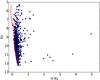 |
Fig. 1 Color magnitude diagram of the observed targets in the Cha I region based on photometry from the Two Micron All Sky Survey (Skrutskie et al. 2006); the 10 Myr isochrone from the Siess et al. (2000) models is overplotted. |
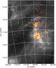 |
Fig. 2 Far infrared (140 μm) map of the region around the young cluster Cha I from the AKARI all-sky survey (Doi et al. 2015). Yellow dots indicate the positions of all the known members from the literature, while the bigger red dots indicate the positions of all the members selected by the GES observations according to the criteria discussed in Sect. 3. The dashed blue circles (centers RA1 = 167.2°, Dec1 = –76.5°, RA2 = 167.2°, Dec2 = –77.5°, and radius 0.35°) delimit the north and south subclusters (see Sects. 4.2 and 5.3). |
We observed a total of 674 stars with GIRAFFE and 49 with UVES (3 in common between the two spectrographs), of which 113 are known members of the cluster on the basis of catalogues reported in the literature (Luhman 2004a, 2007; Luhman et al. 2008). Most of the known members were excluded because they were too faint to be observed with FLAMES. Several fibers were allocated to the sky in order to allow a good background subtraction. Observations were carried out during three different runs between March and May 20121 using the HR15N setup (R ~ 17 000, Δλ = 647−679 nm) for GIRAFFE and the 580 nm (R ~ 47 000, Δλ = 480−680 nm) setup for UVES. The median signal-to-noise ratio of the final spectra is 58 and 62 for GIRAFFE and UVES spectra, respectively.
All GES data were reduced and analyzed using common methodologies and software to produce a uniform set of spectra and stellar parameters, which is periodically released to all the members of the consortium via a science archive2. In this paper, we only use data from the third internal data releases (GESviDR3) of February 2015, with the exception of errors on the GIRAFFE RVs, which are calculated on the basis of the empirical formulae provided by Jackson et al. (2015).
The methodologies used for the data reduction and the derivation of RVs are described in Sects. 2.2 and 2.3 of Jeffries et al. (2014) for the GIRAFFE data, and in Sacco et al. (2014) for the UVES data. Lanzafame et al. (2015) describes in detail the procedures used to derive the stellar paramaters (i.e., effective temperature and gravities), accretion indicators (e.g., Hα width at 10% of the peak – Hα10%), and the equivalent width of the Li line at 6708 Å (hereafter EW(Li)).
3. Membership selection
A detailed selection of members among the stars observed with UVES has been carried out by Spina et al. (2014), who confirmed all the known members from the literature and did not find any new members; therefore, we will only focus on stars observed with GIRAFFE.
Since all the stars formed in the same region have very similar velocities, spectroscopic measurements of the RVs are often considered one of the most robust tools for selecting the members of a cluster. However, one the main goals of this work is to study the dynamical properties of Cha I (e.g., the RV dispersion, the presence of multiple populations); therefore, we use the RVs only to discard the obvious non-members, namely the stars outside of the range 0 < RV < 30 km s-1; for a more accurate selection of the cluster members, we use three independent spectroscopic parameters included in the GES database: the gravity index γ, the EW(Li), and the Hα10%. The major source of contamination within a sample of candidate members of a nearby young cluster selected on the basis of photometric data are background giants. The giants can be identified using the surface gravity index γ, defined by Damiani et al. (2014) with the specific goal of measuring gravities using the GES GIRAFFE spectra observed with the HR15N setup. The upper panel of Fig. 3 shows γ as a function of the effective temperature for the GES targets observed in Cha I. The locus of the giant stars is clearly visible in the upper part of the plot, well separated from the main sequence and pre-main sequence stars. As in previous works (Prisinzano et al. 2016; Damiani et al. 2014), we classified as giants all stars with an effective temperature lower than 5600 K and γ > 1.
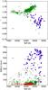 |
Fig. 3 Gravity index γ and EW(Li) as a function of the stellar effective temperature (upper and lower panel, respectively). The index γ and the EW(Li) measured from the GES spectra are indicated with circles: the empty green circles are the non-members, the filled blue circles are the cluster members, and the red dots represent the members already known from previous studies. Upper limits are indicated by red downward arrows. Median error bars are shown on the left for both panels. The black crosses in the bottom panel are the EW(Li) measured for stars in the 30−50 Myr open cluster IC 2602 by Randich et al. (1997, 2001). In both panels, the dashed red lines indicate the threshold used to separate members and non-members. In the bottom panel, a few stars that are above the dashed red line are reported as non-members because they have been excluded according to the criterion based on the gravity index, and other stars that are below this line are classified as members because they are strong accretors, as discussed in Sect. 3. |
After the giants stars are excluded, we need to exclude stars older than Cha I located in the foreground. The most powerful tool for performing this selection is the EW(Li), since late-type stars rapidly deplete their photospheric lithium after 5−30 Myr (e.g., Soderblom 2010). At constant age, the EW(Li) depends on the effective temperature; therefore, we cannot define a single threshold for the whole sample. The lower panel of Fig. 3 shows the EW(Li) as a function of Teff for the observed stars in Cha I and for the stars of the 30−50 Myr open cluster IC 2602 observed by Randich et al. (1997, 2001). We select as cluster members all the stars with EW(Li) above the dashed line in the lower panel of Fig. 3, which represents the upper envelope of the of the EW(Li) measured for the stars belonging to IC 2602. In a few cases, when the EW(Li) but not the effective temperature is derived from the GES spectra (see Lanzafame et al. 2015, for details), we assume the highest threshold (EW(Li) = 300 Å). However, the EW(Li) can be underestimated in stars with a very strong mass accretion rate, because of the continuum emission in excess produced by the accretion shock (e.g., Palla et al. 2005; Sacco et al. 2007); therefore, we include in the sample of members all the stars that can be classified as accretors according to the criterion based on the width at 10% of the peak of the Hα line (Hα10% > 270 km s-1) defined by White & Basri (2003). In the bottom panel of Fig. 3 the cluster members are indicated with filled blue circles. The members below the dashed line have been included because of the Hα10%, while the non-members above the line have been excluded because of the gravity index γ.
Using these criteria, we selected as members of Cha I 89 stars observed with GIRAFFE. This sample includes 7 new members and 82 known members from the literature. Fourteen known members do not meet the membership criteria. Seven of them were excluded because they are out of the range of RVs (0 < RV < 30 km s-1). However, all these stars are strong accretors (Hα10% > 300 km s-1); therefore, the RV derived by the GES pipeline could be incorrect owing to the presence of strong emission lines produced by material moving at a different velocity with respect to the photosphere. We use these stars for the analysis of the structural properties of the cluster (see Sect. 4), but we exclude them from the analysis of the dynamical properties, which is based on the RVs. Six known members were excluded because the SNR < 10 is too low to derive EW(Li) and Hα10% (see Lanzafame et al. 2015), but there is no evidence suggesting that these stars are not members, and so we include them in the final catalogue. Finally, the star HD 97 300 is too hot (SpT = B9) to exhibit the Li absorption feature at 6708 Å, but it is surrounded by a ring of dust due to a bubble blown by the star (Kóspál et al. 2012). This proves that it belongs to the Cha I star-forming region and can be included in the catalogue of members used for the analysis discussed in the following sections. To summarize, the final catalogue of members includes 103 stars (96 already known and 7 new) observed with GIRAFFE and 17 stars observed with UVES (discussed in Spina et al. 2014) for a total of 120 members. We note that our analysis proves that the seven new members are young stars, but does not demonstrate that they belong to Cha I since they could be members of the two young stellar associations ϵ Cha and η Cha, which are slightly older (4−9 Myr, Torres et al. 2008), have similar radial velocities, and are located in the foreground of Cha I. As shown by Lopez Martí et al. (2013b, see Fig. 1 in that paper), the two associations can be easily separated from Cha I using tangential motions, so we retrieved the proper motions of these stars from the UCAC 4 (Zacharias et al. 2013) and, when not available, from the PPMXL (Roeser et al. 2010) catalogues. We found that all the new members have tangential motions consistent with the Cha I cluster except one star (GES ID. 10563146-7618334), which is closer to the ϵ Cha association.
The list of cluster members and the data used for the membership selection are reported in Table 1, while their positions are plotted on the map in Fig. 2 (red dots) together with all the known members of the clusters compiled from the literature (yellow dots). The number of new members does not significantly increase the population of Cha I. However, they belong to the sparse population located in the outer region surrounding the main cloud. So our study proves that this outer population is richer than previously thought.
4. Structural properties
Several studies have shown that a knowledge of the structural properties of open clusters is fundamental in order to understand their origin, their dynamical evolution, and the effects of the star formation environment on the properties of stars and planetary systems (e.g., Scally & Clarke 2002; Schmeja et al. 2008; Allison et al. 2010; Moeckel & Bate 2010; Malmberg et al. 2011; Kruijssen et al. 2012; Parker et al. 2014). In this work we focus on three structural properties: the level of substructure, the stellar density, and the mass segregation.
4.1. Sample and stellar masses
The sample of stars used for the structural analysis includes all the previously known members (observed or not by GES) and the new members discovered by GES. We excluded stars with AJ> 1.2 because catalogues available in the literature are not complete for higher extinction (Luhman 2007).
For the analysis of the mass segregation, we derived homogeneous estimates of stellar masses from the positions of stars in the HR diagram plotted in Fig. 4, using the pre-main sequence evolutionary models developed by Tognelli et al. (2011, 2012). We decided to use these models instead of those provided by Siess et al. (2000) and recommended by the Gaia-ESO guidelines for the target selection process because they have been more recently updated. No masses have been estimated for stars cooler than 3000 K, younger than 0.5 Myr, and older than 20 Myr (i.e., above/below the upper/lower isochrones plotted in the HR diagram). Very cool and very young stars were excluded because mass estimation based on pre-main sequence evolutionary models can be very uncertain. Stars located below the 20 Myr isochrone were excluded because, as suggested by Luhman (2007), Luhman & Muench (2008), their luminosity is underestimated due to the presence of a circumstellar disk seen edge-on, which absorbs most of the photospheric emission.
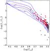 |
Fig. 4 HR diagram of members in Cha I selected from the literature and the GES data with AJ < 1.2 and Teff > 3000 K. Temperatures and luminosities have been derived from the GES spectra and the 2MASS photometry for the red dots, and from the literature for the other stars. Isochrones (at 0.5, 1.5, 3.0, 5.0, 10.0, and 20.0 Myr) and tracks (at 0.1, 0.2, 0.3, 0.6, 1.0, 1.8, 2.4, and 3.0 solar masses) from an improved version of the Tognelli et al. (2011, 2012) pre-main sequence evolutionary models are reported with continuous blue and dashed red lines, respectively. |
To build the HR diagram we used 2MASS photometry and the GES parameters when available, otherwise we used the parameters from Luhman (2004a, 2007). Specifically, the effective temperatures were directly measured from the GIRAFFE and UVES spectra (Lanzafame et al. 2015) in the GES sample and from low-resolution spectra for the other stars (Luhman 2004a, 2007). A comparison of the effective temperatures derived by the GES spectra and those obtained from low-resolution spectroscopy is reported in Fig. 5, which shows that the latter are slightly lower, i.e., in the range between 3600 and 4600 K. We believe that this systematic discrepancy can either be due to the scale used by Luhman (2004a, 2007) to convert spectral types into temperature (GES temperatures are derived directly from the spectra) or to the different spectroscopic resolution of the spectra used for the analysis.
Luminosities were derived from the 2MASS J magnitude corrected for absorption, using the bolometric correction reported in Pecaut & Mamajek (2013) and assuming a distance of 160 pc. For the GES sample, we calculated the absorption AJ from E(J−H) = (J−H)−(J−H)0, assuming AJ/E(J−H) = 0.38 as in Luhman (2004a). The intrisic color (J−H)0 was calculated from the effective temperature using the color-temperature trasformations from Pecaut & Mamajek (2013). For stars that do not belong to GES catalogues, the infrared absorption was retrieved from Luhman (2007, 2004b). The masses of the stars used for the structural analysis are reported in Table 2.
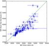 |
Fig. 5 Comparison between the effective temperature retrieved from the literature (y-axis) and measured from the GES spectra (x-axis). |
To understand if the use of different catalogues for the estimation of masses can affect our results, we performed all our analyses only using data from the literature for all the known members; we find no relevant differences. We stress that in the context of this paper the stellar masses are only used to study the level of the mass segregation (see Sects. 4.3 and 4.4). For this scope, we do not need the specific values of the masses, but only to put them in order from the most to the least massive.
Known cluster members from the literature and new members used to study the structural properties of the cluster.
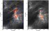 |
Fig. 6 Spatial distribution of the stars (left panel) and starless cores (right panel) used to calculate the Q parameter. The minimum spanning tree is plotted with a yellow line. The blue dashed lines in the left panel show the elliptic boundaries of the regions including the stars used to calculate the values of the Q parameter reported in Fig. 7. |
4.2. Level of substructure
To measure the level of substructure, we use the Q-parameter introduced by Cartwright & Whitworth (2004). This parameter is defined as the ratio  (1)where
  is the mean length of the edges of the minimum spanning tree (MST) connecting the stars, normalized by the factor (NA)1/2/ (N−1) (N is the total number of stars and A is the area of the cluster), and
  is the mean separation between the stars divided by the cluster radius3. Several simulations demonstrate that clusters with Q> 0.8 are characterized by a smooth radially concentrated structure, which is probably the result of dynamical evolution occurring after the cluster formation, while clusters with Q< 0.8 are characterized by a high level of substructure and closely resemble the filamentary structure of the molecular clouds where they formed (e.g., Schmeja & Klessen 2006; Parker & Meyer 2012). To calculate the best estimator
  and the standard error
  of the Q-parameter, we use the Jackknife method (Quenouille 1949; Tukey 1958). This is a resampling method that consists in calculating the value of Qi for N different samples composed of all the stars except for the ith star (with i from 1 to N). The best estimator and the standard error are equal to
 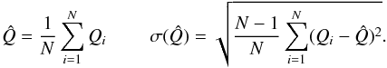 (2)The relation between Q and the level of substructure has been calculated by Cartwright & Whitworth (2004) through simulations considering isotropic clusters. However, Cartwright & Whitworth (Cartwright & Whitworth (2009)) pointed out that in elongated clusters Q could be biased towards lower values, and estimated a correction factor that depends on the cluster aspect ratio. Since Cha I is characterized by a slightly elongated structure, we applied these corrections on our results.
For our sample, the resulting  is higher than that found by previous studies carried out by Cartwright & Whitworth (2004) and Schmeja & Klessen (2006) (Q = 0.68 and 0.67, respectively). Cartwright & Whitworth (2004) did not consider the elongation in their calculation, but this does not explain such a large discrepancy since the elongation factor for our sample is just 1.03. Therefore, this discrepancy is most likely due to the different sample of members used for the calculations. In fact, Cartwright & Whitworth (2004) used the sample of members selected by Lawson et al. (1996) and Ghez et al. (1997), while the Schmeja & Klessen (2006) results are based on a sample of members retrieved from Cambresy et al. (1998). Both samples are less complete and cover a smaller area of the sky than ours. As discussed in the previous section, Cha I is composed of an inner denser region characterized by the presence of a molecular cloud still forming stars and an outer sparser region with no gas. Furthermore, our discovery of new members only in the outer part of the cluster proves that the level of completeness of the star catalogue in the outer region is lower than in the inner one. To understand how this can affect the Q-parameter, we calculated Q for four different samples composed of stars enclosed within the area of the sky delimited by ellipses with the same center (RA = 167.2°, Dec = −77.1°) and eccentricities (e = 0.89), but different semi-major axes (see Table 3 and the left panel of Fig. 6). In particular, the smallest ellipse contains only the stars in the inner embedded region, the largest includes all the stars, and the two intermediate ones have semi-major axes two and four times the smallest.
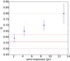 |
Fig. 7 Q-parameter as function of the semi-major axes of the ellipses, shown in Fig. 6, which delimit the area enclosing all the stars used for the calculation. The dotted green line indicates the value of Q expected for a sample of stars randomly distributed, while the continuous and dashed red lines indicate the the Q-parameter with error bars calculated from the positions of the pre-stellar cores. |
Properties of the ellipses used to investigate the relation between Q and the completeness of the member sample.
The value of Q as a function of the semi-major axes of the ellipses is shown in Fig. 7 and is reported in Table 3. The Q-parameter gradually increases from Q ~ 0.6 – when we consider only the stars in the inner and denser region of the cluster – to Q ~ 0.8 for the full sample. This clear correlation between the Q-parameter and the area of the cluster considered to perform the calculation may be due to one or more of the following factors:
-
the stars in the inner region are younger and are located very close to where they formed, so Q is similar to what is expected at the initial stage of the cluster formation (e.g., Parker et al. 2014) when the distribution of stars resembles the distribution of gas in filaments, while the stars in the outer regions migrated from their formation site, so their spatial distribution has been randomized;
-
Cha I is composed of multiple populations with different structural properties. In the different subsets defined by the ellipses, these populations have different weights, so the value of Q changes according to which population weighs the most;
-
the presence of patchy extinction in the inner region produces substructures that would not be present if the full sample of stars were visible;
-
the member selection in the outer regions is not complete. Missing some of the members, we can miss some of the substructures, so Q increases, when we include the outer part of the cluster.
Furthermore, we derived the Q-parameter (Q = 0.56 ± 0.06) from the positions of 60 pre-stellar cores found by Belloche et al. (2011) with a submillimeter survey. The agreement between the value of Q measured for the cores and for the stars in the smaller ellipse supports the explanation given in point a). However, as discussed above the number of objects is too small to consider this measurement statistically robust.
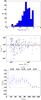 |
Fig. 8 Top: distribution of the surface density Σ and the best-fit model with a lognormal function (continuous red line). Middle: stellar density as defined in Eq. (3) as a function of the star mass. The black and red lines indicate the median density of the whole stellar sample and the ten most massive stars, respectively. The continuous lines represent the best value, while the dashed lines represent their error bars. Bottom: evolution of the mass segregation ratio, ΛMSR, for the NMST most massive stars. The top x-axis indicates the lowest mass star mL within NMST and the dashed line corresponds to ΛMSR = 1, i.e., no mass segregation. |
4.3. Stellar density
The stellar density is a key parameter used to derive the effects of the environment on the evolution of the star-disk systems and the dynamical status of the clusters. To derive the surface density Σ we used the same definition as in Bressert et al. (2010) (3)where N is the Nth nearest neighbor and DN is the projected distance to that neighbor. For our calculation we set N = 7 as in Bressert et al. (2010). The top panel in Fig. 8 shows the density distribution of the stars used to calculate the Q parameter with the best fit of the distribution with a log-normal function (peak ~8 stars pc-2 and dispersion σlog 10Σ = 0.67). The profile of the distribution is very similar to that observed by Bressert et al. (2010; see their Fig. 1) and is well described by a log-normal function in the low-density tail, while at high density the observed distribution decreases faster than a log-normal function. The reason for this deviation from the log-normal model is not clear. However, a similar deviation is also observed in the much larger sample analyzed by Bressert et al. (2010). The peak of the distribution is located at lower densities and the dispersion is lower with respect to the results found by Bressert et al. (2010), but this is not surprising since ~70% of the young stellar objects used for their analysis belong to the Orion star-forming region, which is more massive and much denser than Cha I.
Simulations describing the dynamical evolution of young star clusters suggest that the stellar density may depend on stellar mass, i.e., the density of stars near massive objects can be higher because massive stars act as a potential well and trap low-mass stars (e.g., Parker et al. 2014). The relation between density and mass is plotted in the middle panel of Fig. 8, which shows that the density around the most massive stars (median density  ) is consistent within errors with the surface density for the rest of the stars (median density
  )4. This result proves that either the cluster did not go through a sufficient dynamical evolution to determine an increase in density around the most massive stars or that these stars are not massive enough to act as a potential well and to attract low-mass stars.
4.4. Mass segregation
The last structural property to analyze is the amount of mass segregation. In mass-segregated clusters, the more massive stars are concentrated in a smaller volume (or projected area on the line of sight) than lower mass stars. To estimate the level of mass segregation we used the method introduced by Allison et al. (2009) and based on the mass segregation ratio ΛMSR,  (4)where lsubset is the length of the MST of a subset of stars composed of a number NMST of the most massive stars in the cluster, and laverage is the average of the lengths of the MSTs of 50 different subsets composed of a number NMST of random stars. If ΛMSR > 1, the MST of the more massive stars is smaller than the MST of a random sample so the cluster is mass-segregated; otherwise, if ΛMSR < 1, it is inversely mass segregated (i.e., the most massive stars are spread over a larger area than other stars). To estimate the uncertainties on this ratio, we used the same method as in Parker et al. (2012), namely we considered as lower (upper) error the length of the MST, which lies at 1/6 (5/6) of an ordered list including all the MSTs of the random subsets used to calculate laverage. In the bottom panel of Fig. 8 we show the evolution of ΛMSR as a function of NMST. The upper x-axis shows the smallest mass within the sample of NMST stars. The plot shows only marginal evidence of mass segregation, which is not significant since the value of ΛMSR at higher masses is consistent with ΛMSR = 1, and ΛMSR for intermediate mass stars is above 1 by less than 2−3 error bars, which as estimated by simulations performed by Parker & Goodwin (2015) means a significance lower than 95%.
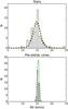 |
Fig. 9 Top: RV distribution of the full sample of cluster members observed by GES. The red and green dashed lines describe the best-fit models with a Gaussian broadened by the measurement errors and the velocity offsets due to binaries, assuming a fixed binary fraction (fbin = 0.5) and leaving the binary fraction free to vary, respectively. Bottom: distribution of the RVs of the pre-stellar cores measured by Tsitali et al. (2015) from the C18O (2−1) molecular transition, with the best-fit models with a Gaussian function superimposed. |
5. Kinematical properties
The precision of the RVs derived from the GES spectra (Jackson et al. 2015) allows us to study the kinematical properties of the cluster. We will use the RVs to determine its global RV dispersion σc, to investigate the presence of a RV gradient, and to understand if the two different populations identified by Luhman et al. (2008) have different kinematical properties. For this analysis, we will only use members of the cluster observed by GES and reported in Table 1 because we only have precise measurements of the RV with a proper evaluation of the errors for these stars.
Parameters obtained from the fits of the RV distributions with 1σ errors.
5.1. Radial velocity dispersion
The RV distribution of the cluster members is shown in the top panel of Fig. 9. We modeled the distribution using a maximum-likelihood method developed by Cottaar et al. (2012b) and already used in several works (e.g., Jeffries et al. 2014; Foster et al. 2015; Sacco et al. 2015), which allows us to properly take into account the errors on each star and the presence of binaries. Specifically, we assume that the stellar RVs have an intrinsic Gaussian distribution (with mean vc and standard deviation σc) broadened by the measurement uncertainties and the velocity offsets due to binary orbital motion. The distribution of the offsets is calculated numerically by a code5 developed by Cottaar et al. (2012b) that makes three different assumptions: a) binary periods follow a log-normal distribution with mean period 5.03 and dispersion 2.28 in log 10 days (Raghavan et al. 2010); b) the secondary-to-primary ratio (q) follows a power law  for 0.1 < q < 1 (Reggiani & Meyer 2011); and c) the distribution of eccentricities is flat between 0 and a maximum value that depends on the period according to Eq. (6) from Parker & Goodwin (2009).
 |
Fig. 10 From top to bottom: RV distributions of the north subcluster, the south subcluster, and the stars dispersed in the outer regions. The dashed blue line marks the velocity of 15 km s-1 and the red line is the best-fit distribution with the same model used for the full sample. |
We performed two fits. In the first (fit 1 in Table 4), we kept the fraction of binaries fixed at fbin = 0.5, while in the second (fit 2 in Table 4), it was left free to vary. In both fits, we only consider stars in the range 0 < RV < 30 km s-1 since stars outside this range are either binaries or stars with a miscalculated RV due to the presence of strong emission lines. The parameters derived by the two fits are reported in the first two rows of Table 4 and the best-fit functions are plotted in Fig. 9. Since the two models are nested, to evaluate the parameters of which fit to adopt we can perform a likelihood-ratio test. This gives a probability P(Lfit1/Lfit2) = 3.8%, which indicates, with a marginal level of significance, that the fit with a fixed binary fraction can be rejected and the parameters from the second fit can be adopted.
Our results are in agreement with previous estimates of the central cluster velocity and of the velocity dispersion from Joergens (2006; vc = 14.7 km s-1 and σc = 1.3 km s-1).
5.2. Radial velocity gradient
To investigate the presence of a RV gradient in the stellar population, we fitted the RV distribution with the same function discussed in the previous section, but instead of considering the mean cluster velocity vc as a single free parameter, we assumed that the velocity vc = vc0 + αΔRA + βΔDec, where ΔRA and ΔDec are the RA and Dec shifts of each star with respect to a fixed position calculated as the median of the star positions, and vc0, α, and β are free parameters of the fit together with σc, which is assumed to be constant over the whole region. The result of this fit is reported in Table 4 (fit 3). The parameters vc0 and σc are in agreement with the results found with the previous fits and the components of the RV gradient α and β are consistent within two standard deviations with zero. Since the function used for fit 2 is the same as fit 3 when we fix the parameters α and β to zero, we can use the likelihood-ratio test to compare the model with and without a gradient. The probability P(Lmax(fit2) /Lmax(fit3)) = 26%, so we conclude that there is no evidence of the presence of a RV gradient in the cluster.
5.3. Kinematical properties of the subclusters
Luhman (2007) suggested that Cha I is composed of two subclusters with different star formation histories. To understand if these two populations have different kinematical properties we divided our sample in three groups: the first composed of 29 stars located within the upper circle (see Fig. 2, blue dashed line), which approximately defines the boundary of the northern part of the cloud; the second composed of 37 stars within the lower circle, which defines the boundary of the southern cloud; and the third composed of 25 stars located in the outer regions.
The RV distributions of the three samples are shown in Fig. 10 and the results from the fits of the distributions are reported in the last rows of Table 4. The central RVs of the two clusters concentrated around the clouds differ by ~1 km s-1 at 2σ level of significance; on the basis of a Kolmogorov-Smirnov test the probability that the two distributions are part of the same population is <1%. The kinematical properties of the stars located in the outer regions are closer to those found for the northern stars, suggesting that the majority of the outer stars belong to the northern cluster. This is consistent with the hypothesis suggested by Luhman (2007) that the northern cluster started to form earlier and therefore that it is going through a more advanced stage of its evolution. Lopez Martí et al. (2013b) already tried to kinematically separate the two subclusters using proper motions, finding no evidence of different velocities. They do not report any upper limit on the velocity separation between subclusters, so it is difficult to compare their data with our result. However, the precision of proper motions used for their work is lower than RVs from the Gaia-ESO Survey.
6. Discussion
The main goal of this work is to study the physical processes leading to the formation and the dynamical evolution of small star clusters. In the next sections, we compare the structural and dynamical properties of the stellar populations in Cha I with the properties of pre-stellar cores and with some numerical models describing the early stages of the star cluster evolution.
6.1. Structural properties
Using N-body simulations, Parker et al. (2014) studied the evolution of the level of substructure and the mass segregation in young star clusters. In Fig. 11 we compare the results of the simulations performed by Parker et al. (2014) for clusters with high (nstars ~ 1000 stars pc-1) and low (nstars ~ 100 stars pc-1) stellar density with the structural properties of Cha I derived in Sect. 4. The simulations differ for the initial virial ratio (αvir) and the initial fractal dimension D, which indicates that the level of substructure (D = 1.6 is a highly substructured cluster and D = 3.0 is a roughly uniform sphere). The figure shows the initial conditions of the simulated clusters (t = 0 Myr) and their status after 2 Myr.
None of the simulated clusters with high stellar density reproduces the structural properties of Cha I, with the exception of the case of a supervirial cluster with no substructure. However, even in this case, the properties of the simulated clusters at the initial conditions are not consistent with the properties of the pre-stellar cores. This result is not surprising; the stellar density of the simulated clusters is much higher than the observed density in Cha I of both stars and pre-stellar cores, and further supports the hypothesis that Cha I did not form in a high-density environment, in contrast to the hypothesis advanced by Marks & Kroupa (2012).
The properties of the low-density simulated clusters are much closer to the properties of Cha I. In particular, virial and supervirial simulated clusters are consistent with the overall properties of the cluster after 2 Myr of dynamical evolution. Furthermore, the simulations with a high level of substructure at t = 0 Myr are consistent with the properties of embedded stars and pre-stellar cores, if we assume that they represent the properties of the cluster at its formation. Otherwise, according to the simulations, for a cluster which is initially subvirial we should observe a level of mass segregation after 2 Myr, which we do not observe in Cha I.
To summarize, according to this analysis, Cha I formed in a low-density environment with a virial ratio αvir ≥ 0.5 and a high level of substructure. It has erased substructure due to dynamical interactions and will likely disperse in the Galactic field. A similar scenario has been proposed for the more evolved cluster Gamma Velorum (Jeffries et al. 2014; Mapelli et al. 2015; Sacco et al. 2015). It would be interesting to perform a direct measurement of the virial ratio in Cha I. However, owing to the highly asymmetric structures of the stellar and gas components of the cluster, it is difficult to estimate the virial ratio without any information about its structure along the line of sight. This information will be provided by the astrometric mission Gaia for most of the optically visible stars.
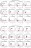 |
Fig. 11 Comparison between the observed structural properties of Cha I and simulated clusters with high (nstars = 1000 stars pc-3, top panels) and low (nstars = 100 stars pc-3, bottom panels) initial stellar density from Parker et al. (2014). The panels on the left and on the right show the Q-parameter as a function of ΣLDR (i.e., the ratio between the median superficial density of the most massive stars and the rest of the sample) and ΛMSR (for the ten most massive stars), respectively. The simulations differ for the initial virial ratio αvir and the initial level of substructure (D = 1.6 is a highly substructured cluster and D = 3.0 is a roughly uniform sphere). Blue crosses and black circles represent the simulated clusters at the initial conditions and after 2 Myr evolution, respectively. Green and black dots represent the properties of Cha I for the full sample of members and only for the stars in the embedded region within the smallest ellipse in Fig. 6, respectively. The red lines trace the Q-parameter estimated for the pre-stellar cores with errors. |
It is worth mentioning a few caveats concerning the comparisons between the simulations performed by Parker et al. (2014) and our results. First, as proven by the large area of the parameter space covered by the simulations in each panels of Fig. 11, N-body simulations, especially of low-density clusters, are partially degenerate; in other words, the same initial conditions may lead to clusters with very different properties in the Q vs. ΣLDR and Q vs. ΛMSR plots. In particular, the comparison between our results and models strongly constrains the initial density of the cluster, but constrains other critical properties, like the initial virial ratio, to a lesser degree. The analysis of other young star clusters similar to Cha I and the definition of new diagnostics of the dynamical status of star clusters that also use kinematic data can help to overcome this limitation. In addition, N-body simulations do not include the presence of gas, which in the case of Cha I is the main component of the potential energy of the systems. The effects of the gas in the evolution of star clusters is a very debated topic. Some authors (e.g., Kruijssen et al. 2012) suggest that the influence of the gas in the cluster dynamics is negligible, but a direct comparison between simulations describing in a consistent way the evolution of gas and stars is required to provide final answers to this issue. Finally, the simulations discussed in this paper assume that all the stars are coeval, while the age spread in Cha I is larger than its median age. The origin of the age spread in young clusters is not clear and is not reproduced by any of the state-of-the-art simulations. More sophisticated simulations and precise and complete data are required to fully understand the star formation history of clusters like Cha I.
6.2. Kinematical properties
As shown in Fig. 9, the clearest result of the kinematical analysis is the large discrepancy between the velocity dispersion of the stars (σstars = 1.10 ± 0.15 km s-1) and that of pre-stellar cores (σcores ~ 0.3 km s-1) derived from submillimeter observations of molecular transitions by Tsitali et al. (2015). As noted in Table 4, the velocity dispersion of the stellar component does not depend on the sample of stars used for the fit. In fact, the two subclusters around the molecular cloud and the sample of stars located in the outer region have similar velocity dispersions, which are in all cases much higher than the dispersion measured for the pre-stellar cores. A similar discrepancy between the pre-stellar cores and the stars has been observed in the ρ Oph star-forming region, in the young cluster NGC 1333, and in Orion. The velocity dispersion of the stellar component in ρ Oph (σstars = 1.14 ± 0.35 km s-1) was derived from the Gaia-ESO observations of the optically visible stars around the main cloud L1688 by Rigliaco et al. (2016), who suggested that the cluster is bound and in virial equilibrium, while the velocity dispersion of the cores (σcores ~ 0.4 km s-1) was estimated by André et al. (2007), who suggested that the cores are subvirial. The kinematical properties of both the cores and the stars of NGC 1333 have been analyzed by Foster et al. (2015), who also found that the stars are virial (σstars = 0.92 ± 0.12 km s-1), while the cores (σcores ~ 0.5 km s-1) are subvirial. They suggested that the discrepancy between stars and cores can either be due to the magnetic field having a strong influence on the cores and/or to the global collapse of the cluster after the protostellar phase. A similar conclusion has been obtained via N-body simulations carried out by Parker & Wright (2016), who found that clusters starting as subvirial undergo cool collapse, so the dynamical interaction among stars quickly inflate the distribution. However, for small low-density clusters Parker & Wright (2016) found a lower velocity dispersion (σ ~ 0.5 km s-1) than observed. This discrepancy could be associated with the lack of gas in the N-body simulations since the presence of a significant amount of gas reduces the virial ratio and leads to the collapse of clusters with higher velocity dispersion than in the case without gas (Leigh et al. 2014; Mapelli et al., in prep.). The morphology and the kinematics of gas, protostars, and pre-main sequence stars have been studied in Orion A by Stutz & Gould (2016). They propose that protostars are ejected from the filaments by magnetically induced transverse waves. This slingshot-like mechanism is responsible for the velocity discrepancy between young stars and protostars still within the filaments.
The second result of our kinematical analysis is the discrepancy (~1 km s-1) between the central velocities of the two subclusters located around the northern and southern clouds. This is not surprising because Luhman (2007) suggested that Cha I is composed of two components with different star formation histories. Furthermore, recent studies show that multiple populations (e.g., Jeffries et al. 2014; Sacco et al. 2015) and RV gradients (e.g., Tobin et al. 2015) are common in young clusters and star-forming regions. According to the submillimeter observations, the mean velocities of the cores in the north and the south clusters also differ by ~0.3 km s-1. However, the discrepancy is in the opposite direction with respect to what we found for the stars; i.e., the cores in the south have a higher redshift than in the north. The reason for this anti-correlation between stars and cores is not clear, but this result supports a scenario where the dynamics of the cores is independent of the dynamics of the stellar populations.
7. Conclusions
In this work we present a new analysis of the spectroscopic parameters derived from the Gaia-ESO Survey observations of the young cluster Cha I aimed at investigating the structural and dynamical properties of the cluster. We obtained the following main results.
-
1.
An evident discrepancy between the velocity dispersion of the stellar component (σstar = 1.10 ± 0.15 km s-1) derived using the Gaia-ESO spectra and the dispersion (σcores = 0.3 km s-1) of pre-stellar cores derived using submillimeter observations. A similar discrepancy has been observed in the young embedded clusters ρ Oph and NGC 1333, and in Orion. The origin of such a large discrepancy is not clear. It could be related to the effect of the magnetic field on the protostars or the filaments where they form, or to two-body stellar dynamical interactions following the cluster formation. We will investigate this issue further in a forthcoming paper (Mapelli et al., in prep.).
-
2.
Analyzing independently the RV distributions of the two subclusters located around the two main molecular clouds, we found that the central RVs differ by ~1 km s-1. This result supports the evidence found by Luhman (2007) that Cha I is composed of two subclusters with different star formation histories and a scenario where young clusters do not form as monolithic systems, but from the merging of smaller subsystems.
-
3.
A new membership analysis based on three independent spectroscopic criteria led to the confirmation of all the previously known members, for which new astrophysical parameters from the Gaia-ESO Survey are available, and to the discovery of six new members in Cha I and one new member of the ϵ Cha association, which are all located in the outer part of the cluster.
-
4.
The level of substructure of the cluster measured using the Q-parameter defined by Cartwright & Whitworth (2004) depends on the sample used for the calculation. If we consider only the stars in the inner region, the value of Q indicates that the cluster is highly substructured; instead, if we take into account the full sample of members, the spatial distribution of the cluster is consistent with a random sample. It is not clear whether this trend has a physical origin or is the result of a bias due to differential extinction in the inner region of the cluster or incomplete target selection in the outer region.
-
5.
As observed in other low-mass young star clusters, Cha I is not mass-segregated and its superficial density follows a log-normal distribution, with the exception of its high-mass end, which follows a steeper trend.
-
6.
The comparison between the observed structural properties of Cha I and the results of N-body simulations performed by Parker et al. (2014) suggests that the cluster formed as highly substructured, and virial or supervirial. However, discrepancies between the simulated clusters and Cha I (e.g., the lack of gas in the simulated clusters) may affect this comparison.
Technical details of the fiber allocation procedure and observations are discussed in Bragaglia et al. (in prep.).
The GES science archive is run by the Royal Observatory of Edinburgh. More information on the archive is available at the website http://ges.roe.ac.uk
The radius and the area of the cluster are calculated as described in Cartwright & Whitworth (2004). Specifically, the former is the distance between the center of the cluster and the most distant stars, and the latter is the area of a circular surface with the same radius.
The best values and the error bars of the densities were calculated by generating 2000 bootstrap resamples. Namely, the best value is the median of the bootstrap distribution, while the lower and upper values defined by the error bars correspond to the 15th and 85th percentiles.
Available online at https://github.com/MichielCottaar/velbin
Acknowledgments
These data products have been processed by the Cambridge Astronomy Survey Unit (CASU) at the Institute of Astronomy, University of Cambridge, and by the FLAMES/UVES reduction team at INAF/Osservatorio Astrofisico di Arcetri. These data have been obtained from the Gaia-ESO Survey Data Archive, prepared and hosted by the Wide Field Astronomy Unit, Institute for Astronomy, University of Edinburgh, which is funded by the UK Science and Technology Facilities Council. This work was partly supported by the European Union FP7 programme through ERC grant number 320360 and by the Leverhulme Trust through grant RPG-2012-541. We acknowledge the support from INAF and Ministero dell’Istruzione, dell’Università e della Ricerca (MIUR) in the form of the grant “Premiale VLT 2012”. This work has been partially supported by PRIN-INAF-2014. The results presented here benefited from discussions held during the Gaia-ESO workshops and conferences supported by the ESF (European Science Foundation) through the GREAT Research Network Programme. M.M. acknowledges financial support from the Italian Ministry of Education, University and Research (MIUR) through grant FIRB 2012 RBFR12PM1F, from INAF through grant PRIN-2014-14, and from the MERAC Foundation. S.G.S. acknowledges the support by Fundação para a Ciência e Tecnologia (FCT) through national funds and a research grant (project Ref. UID/FIS/04434/2013, and PTDC/FIS-AST/7073/2014). S.G.S. also acknowledge the support from FCT through Investigador FCT contract of reference IF/00028/2014 and POPH/FSE (EC) by FEDER funding through the program Programa Operacional de Factores de Competitividade COMPETE.
References
- Allison, R. J., Goodwin, S. P., Parker, R. J., et al. 2009, MNRAS, 395, 1449 [Google Scholar]
- Allison, R. J., Goodwin, S. P., Parker, R. J., Portegies Zwart, S. F., & de Grijs, R. 2010, MNRAS, 407, 1098 [Google Scholar]
- André, P., Belloche, A., Motte, F., & Peretto, N. 2007, A&A, 472, 519 [NASA ADS] [CrossRef] [EDP Sciences] [Google Scholar]
- Banerjee, S., & Kroupa, P. 2014, ApJ, 787, 158 [NASA ADS] [CrossRef] [Google Scholar]
- Baumgardt, H., & Kroupa, P. 2007, MNRAS, 380, 1589 [NASA ADS] [CrossRef] [Google Scholar]
- Belloche, A., Schuller, F., Parise, B., et al. 2011, A&A, 527, A145 [NASA ADS] [CrossRef] [EDP Sciences] [Google Scholar]
- Boulanger, F., Bronfman, L., Dame, T. M., & Thaddeus, P. 1998, A&A, 332, 273 [NASA ADS] [Google Scholar]
- Bressert, E., Bastian, N., Gutermuth, R., et al. 2010, MNRAS, 409, L54 [NASA ADS] [Google Scholar]
- Cambresy, L., Epchtein, N., Copet, E., et al. 1997, A&A, 324, L5 [NASA ADS] [Google Scholar]
- Cambresy, L., Copet, E., Epchtein, N., et al. 1998, A&A, 338, 977 [NASA ADS] [Google Scholar]
- Carpenter, J. M. 2000, AJ, 120, 3139 [NASA ADS] [CrossRef] [Google Scholar]
- Carpenter, J. M., Hillenbrand, L. A., Skrutskie, M. F., & Meyer, M. R. 2002, AJ, 124, 1001 [NASA ADS] [CrossRef] [Google Scholar]
- Cartwright, A., & Whitworth, A. P. 2004, MNRAS, 348, 589 [NASA ADS] [CrossRef] [Google Scholar]
- Cartwright, A., & Whitworth, A. P. 2009, MNRAS, 392, 341 [NASA ADS] [CrossRef] [Google Scholar]
- Cottaar, M., Meyer, M. R., Andersen, M., & Espinoza, P. 2012a, A&A, 539, A5 [NASA ADS] [CrossRef] [EDP Sciences] [Google Scholar]
- Cottaar, M., Meyer, M. R., & Parker, R. J. 2012b, A&A, 547, A35 [NASA ADS] [CrossRef] [EDP Sciences] [Google Scholar]
- Covino, E., Alcala, J. M., Allain, S., et al. 1997, A&A, 328, 187 [NASA ADS] [Google Scholar]
- Damiani, F., Prisinzano, L., Micela, G., et al. 2014, A&A, 566, A50 [NASA ADS] [CrossRef] [EDP Sciences] [Google Scholar]
- Da Rio, N., Tan, J. C., & Jaehnig, K. 2014, ApJ, 795, 55 [NASA ADS] [CrossRef] [Google Scholar]
- Doi, Y., Takita, S., Ootsubo, T., et al. 2015, PASJ, 67, 50 [NASA ADS] [Google Scholar]
- Dubath, P., Reipurth, B., & Mayor, M. 1996, A&A, 308, 107 [NASA ADS] [Google Scholar]
- Elmegreen, B. G. 2008, ApJ, 672, 1006 [NASA ADS] [CrossRef] [Google Scholar]
- Feigelson, E. D., Townsley, L. K., Broos, P. S., et al. 2013, ApJS, 209, 26 [Google Scholar]
- Foster, J. B., Cottaar, M., Covey, K. R., et al. 2015, ApJ, 799, 136 [NASA ADS] [CrossRef] [Google Scholar]
- Frasca, A., Biazzo, K., Lanzafame, A. C., et al. 2015, A&A, 575, A4 [NASA ADS] [CrossRef] [EDP Sciences] [Google Scholar]
- Fűrész, G., Hartmann, L. W., Szentgyorgyi, A. H., et al. 2006, ApJ, 648, 1090 [NASA ADS] [CrossRef] [Google Scholar]
- Fűrész, G., Hartmann, L. W., Megeath, S. T., Szentgyorgyi, A. H., & Hamden, E. T. 2008, ApJ, 676, 1109 [NASA ADS] [CrossRef] [Google Scholar]
- Getman, K. V., Flaccomio, E., Broos, P. S., et al. 2005, ApJS, 160, 319 [NASA ADS] [CrossRef] [Google Scholar]
- Ghez, A. M., McCarthy, D. W., Patience, J. L., & Beck, T. L. 1997, ApJ, 481, 378 [NASA ADS] [CrossRef] [Google Scholar]
- Gilmore, G., Randich, S., Asplund, M., et al. 2012, The Messenger, 147, 25 [NASA ADS] [Google Scholar]
- Goodwin, S. P., & Bastian, N. 2006, MNRAS, 373, 752 [NASA ADS] [CrossRef] [Google Scholar]
- Güdel, M., Briggs, K. R., Arzner, K., et al. 2007, A&A, 468, 353 [NASA ADS] [CrossRef] [EDP Sciences] [Google Scholar]
- Guenther, E. W., Esposito, M., Mundt, R., et al. 2007, A&A, 467, 1147 [NASA ADS] [CrossRef] [EDP Sciences] [Google Scholar]
- Gutermuth, R. A., Megeath, S. T., Myers, P. C., et al. 2009, ApJS, 184, 18 [NASA ADS] [CrossRef] [Google Scholar]
- Haikala, L. K., Harju, J., Mattila, K., & Toriseva, M. 2005, A&A, 431, 149 [NASA ADS] [CrossRef] [EDP Sciences] [Google Scholar]
- Høg, E., Fabricius, C., Makarov, V. V., et al. 2000, A&A, 355, L27 [NASA ADS] [Google Scholar]
- Jackson, R. J., Jeffries, R. D., Lewis, J., et al. 2015, A&A, 580, A75 [NASA ADS] [CrossRef] [EDP Sciences] [Google Scholar]
- Jeffries, R. D., Jackson, R. J., Cottaar, M., et al. 2014, A&A, 563, A94 [NASA ADS] [CrossRef] [EDP Sciences] [Google Scholar]
- Joergens, V. 2006, A&A, 448, 655 [NASA ADS] [CrossRef] [EDP Sciences] [Google Scholar]
- Joergens, V., & Guenther, E. 2001, A&A, 379, L9 [NASA ADS] [CrossRef] [EDP Sciences] [Google Scholar]
- Johnstone, D., Hollenbach, D., & Bally, J. 1998, ApJ, 499, 758 [NASA ADS] [CrossRef] [Google Scholar]
- Kóspál, Á., Prusti, T., Cox, N. L. J., et al. 2012, A&A, 541, A71 [NASA ADS] [CrossRef] [EDP Sciences] [Google Scholar]
- Kroupa, P., Aarseth, S., & Hurley, J. 2001, MNRAS, 321, 699 [NASA ADS] [CrossRef] [Google Scholar]
- Kruijssen, J. M. D., Maschberger, T., Moeckel, N., et al. 2012, MNRAS, 419, 841 [NASA ADS] [CrossRef] [Google Scholar]
- Lada, C. J., & Lada, E. A. 2003, ARA&A, 41, 57 [NASA ADS] [CrossRef] [Google Scholar]
- Lanzafame, A. C., Frasca, A., Damiani, F., et al. 2015, A&A, 576, A80 [NASA ADS] [CrossRef] [EDP Sciences] [Google Scholar]
- Lawson, W. A., Feigelson, E. D., & Huenemoerder, D. P. 1996, MNRAS, 280, 1071 [NASA ADS] [Google Scholar]
- Leigh, N. W. C., Mastrobuono-Battisti, A., Perets, H. B., & Böker, T. 2014, MNRAS, 441, 919 [NASA ADS] [CrossRef] [Google Scholar]
- López Martí, B., Jiménez-Esteban, F., Bayo, A., et al. 2013a, A&A, 556, A144 [NASA ADS] [CrossRef] [EDP Sciences] [Google Scholar]
- Lopez Martí, B., Jimenez Esteban, F., Bayo, A., et al. 2013b, A&A, 551, A46 [NASA ADS] [CrossRef] [EDP Sciences] [Google Scholar]
- Luhman, K. L. 2004a, ApJ, 602, 816 [NASA ADS] [CrossRef] [Google Scholar]
- Luhman, K. L. 2004b, ApJ, 616, 1033 [NASA ADS] [CrossRef] [Google Scholar]
- Luhman, K. L. 2007, ApJS, 173, 104 [Google Scholar]
- Luhman, K. L. 2008, in Handbook of Star Forming Regions, Volume II, ed. B. Reipurth, 169 [Google Scholar]
- Luhman, K. L., & Muench, A. A. 2008, ApJ, 684, 654 [NASA ADS] [CrossRef] [Google Scholar]
- Luhman, K. L., Allen, L. E., Allen, P. R., et al. 2008, ApJ, 675, 1375 [NASA ADS] [CrossRef] [Google Scholar]
- Malmberg, D., Davies, M. B., & Heggie, D. C. 2011, MNRAS, 411, 859 [NASA ADS] [CrossRef] [Google Scholar]
- Mapelli, M., Vallenari, A., Jeffries, R. D., et al. 2015, A&A, 578, A35 [NASA ADS] [CrossRef] [EDP Sciences] [Google Scholar]
- Marks, M., & Kroupa, P. 2012, A&A, 543, A8 [NASA ADS] [CrossRef] [EDP Sciences] [Google Scholar]
- McKee, C. F., & Ostriker, E. C. 2007, ARA&A, 45, 565 [NASA ADS] [CrossRef] [Google Scholar]
- Mizuno, A., Hayakawa, T., Tachihara, K., et al. 1999, PASJ, 51, 859 [NASA ADS] [CrossRef] [Google Scholar]
- Mizuno, A., Yamaguchi, R., Tachihara, K., et al. 2001, PASJ, 53, 1071 [NASA ADS] [CrossRef] [Google Scholar]
- Moeckel, N., & Bate, M. R. 2010, MNRAS, 404, 721 [NASA ADS] [CrossRef] [Google Scholar]
- Monet, D. G., Levine, S. E., Canzian, B., et al. 2003, AJ, 125, 984 [NASA ADS] [CrossRef] [Google Scholar]
- Palla, F., Randich, S., Flaccomio, E., & Pallavicini, R. 2005, ApJ, 626, L49 [NASA ADS] [CrossRef] [Google Scholar]
- Parker, R. J., & Dale, J. E. 2013, MNRAS, 432, 986 [NASA ADS] [CrossRef] [Google Scholar]
- Parker, R. J., & Dale, J. E. 2015, MNRAS, 451, 3664 [NASA ADS] [CrossRef] [Google Scholar]
- Parker, R. J., & Goodwin, S. P. 2009, MNRAS, 397, 1041 [NASA ADS] [CrossRef] [Google Scholar]
- Parker, R. J., & Goodwin, S. P. 2015, MNRAS, 449, 3381 [NASA ADS] [CrossRef] [Google Scholar]
- Parker, R. J., & Meyer, M. R. 2012, MNRAS, 427, 637 [Google Scholar]
- Parker, R. J., & Wright, N. J. 2016, MNRAS, 457, 3430 [NASA ADS] [CrossRef] [Google Scholar]
- Parker, R. J., Bouvier, J., Goodwin, S. P., et al. 2011, MNRAS, 412, 2489 [NASA ADS] [CrossRef] [Google Scholar]
- Parker, R. J., Maschberger, T., & Alves de Oliveira, C. 2012, MNRAS, 426, 3079 [NASA ADS] [CrossRef] [Google Scholar]
- Parker, R. J., Wright, N. J., Goodwin, S. P., & Meyer, M. R. 2014, MNRAS, 438, 620 [NASA ADS] [CrossRef] [Google Scholar]
- Pecaut, M. J., & Mamajek, E. E. 2013, ApJS, 208, 9 [NASA ADS] [CrossRef] [Google Scholar]
- Prisinzano, L., Damiani, F., Micela, G., et al. 2016, A&A, 589, A70 [NASA ADS] [CrossRef] [EDP Sciences] [Google Scholar]
- Quenouille, M. H. 1949, The Annals of Mathematical Statistics, 20, 355 [CrossRef] [Google Scholar]
- Raghavan, D., McAlister, H. A., Henry, T. J., et al. 2010, ApJS, 190, 1 [NASA ADS] [CrossRef] [EDP Sciences] [Google Scholar]
- Randich, S., & Gilmore, G. 2013, The Messenger, 154, 47 [NASA ADS] [Google Scholar]
- Randich, S., Aharpour, N., Pallavicini, R., Prosser, C. F., & Stauffer, J. R. 1997, A&A, 323, 86 [NASA ADS] [Google Scholar]
- Randich, S., Pallavicini, R., Meola, G., Stauffer, J. R., & Balachandran, S. C. 2001, A&A, 372, 862 [NASA ADS] [CrossRef] [EDP Sciences] [Google Scholar]
- Reggiani, M. M., & Meyer, M. R. 2011, ApJ, 738, 60 [NASA ADS] [CrossRef] [Google Scholar]
- Rigliaco, E., Wilking, B., Meyer, M. R., et al. 2016, A&A, 588, A123 [NASA ADS] [CrossRef] [EDP Sciences] [Google Scholar]
- Roeser, S., Demleitner, M., & Schilbach, E. 2010, AJ, 139, 2440 [NASA ADS] [CrossRef] [Google Scholar]
- Rosotti, G. P., Dale, J. E., de Juan Ovelar, M., et al. 2014, MNRAS, 441, 2094 [NASA ADS] [CrossRef] [Google Scholar]
- Sacco, G. G., Randich, S., Franciosini, E., Pallavicini, R., & Palla, F. 2007, A&A, 462, L23 [NASA ADS] [CrossRef] [EDP Sciences] [Google Scholar]
- Sacco, G. G., Morbidelli, L., Franciosini, E., et al. 2014, A&A, 565, A113 [NASA ADS] [CrossRef] [EDP Sciences] [Google Scholar]
- Sacco, G. G., Jeffries, R. D., Randich, S., et al. 2015, A&A, 574, L7 [NASA ADS] [CrossRef] [EDP Sciences] [Google Scholar]
- Sánchez, N., & Alfaro, E. J. 2009, ApJ, 696, 2086 [NASA ADS] [CrossRef] [Google Scholar]
- Scally, A., & Clarke, C. 2002, MNRAS, 334, 156 [NASA ADS] [CrossRef] [Google Scholar]
- Schmeja, S., & Klessen, R. S. 2006, A&A, 449, 151 [NASA ADS] [CrossRef] [EDP Sciences] [Google Scholar]
- Schmeja, S., Kumar, M. S. N., & Ferreira, B. 2008, MNRAS, 389, 1209 [NASA ADS] [CrossRef] [Google Scholar]
- Siess, L., Dufour, E., & Forestini, M. 2000, A&A, 358, 593 [Google Scholar]
- Skrutskie, M. F., Cutri, R. M., Stiening, R., et al. 2006, AJ, 131, 1163 [NASA ADS] [CrossRef] [Google Scholar]
- Soderblom, D. R. 2010, ARA&A, 48, 581 [NASA ADS] [CrossRef] [Google Scholar]
- Spina, L., Randich, S., Palla, F., et al. 2014, A&A, 568, A2 [NASA ADS] [CrossRef] [EDP Sciences] [Google Scholar]
- Stutz, A. M., & Gould, A. 2016, A&A, 590, A2 [NASA ADS] [CrossRef] [EDP Sciences] [Google Scholar]
- Tobin, J. J., Hartmann, L., Fűrész, G., Hsu, W.-H., & Mateo, M. 2015, AJ, 149, 119 [NASA ADS] [CrossRef] [Google Scholar]
- Tognelli, E., Prada Moroni, P. G., & Degl’Innocenti, S. 2011, A&A, 533, A109 [NASA ADS] [CrossRef] [EDP Sciences] [Google Scholar]
- Tognelli, E., Degl’Innocenti, S., & Prada Moroni, P. G. 2012, A&A, 548, A41 [NASA ADS] [CrossRef] [EDP Sciences] [Google Scholar]
- Torres, C. A. O., Quast, G. R., Melo, C. H. F., & Sterzik, M. F. 2008, Young Nearby Loose Associations, ed. B. Reipurth, 757 [Google Scholar]
- Tsitali, A. E., Belloche, A., Garrod, R. T., Parise, B., & Menten, K. M. 2015, A&A, 575, A27 [NASA ADS] [CrossRef] [EDP Sciences] [Google Scholar]
- Tukey, J. W. 1958, The Annals of Mathematical Statistics, 29, 614 [CrossRef] [Google Scholar]
- White, R. J., & Basri, G. 2003, ApJ, 582, 1109 [NASA ADS] [CrossRef] [Google Scholar]
- Whittet, D. C. B., Prusti, T., Franco, G. A. P., et al. 1997, A&A, 327, 1194 [NASA ADS] [Google Scholar]
- Wright, N. J., Parker, R. J., Goodwin, S. P., & Drake, J. J. 2014, MNRAS, 438, 639 [NASA ADS] [CrossRef] [Google Scholar]
- Zacharias, N., Finch, C. T., Girard, T. M., et al. 2013, AJ, 145, 44 [NASA ADS] [CrossRef] [EDP Sciences] [Google Scholar]
All Tables
Known cluster members from the literature and new members used to study the structural properties of the cluster.
Properties of the ellipses used to investigate the relation between Q and the completeness of the member sample.
All Figures
|
Fig. 1 Color magnitude diagram of the observed targets in the Cha I region based on photometry from the Two Micron All Sky Survey (Skrutskie et al. 2006); the 10 Myr isochrone from the Siess et al. (2000) models is overplotted. |
| In the text | |
|
Fig. 2 Far infrared (140 μm) map of the region around the young cluster Cha I from the AKARI all-sky survey (Doi et al. 2015). Yellow dots indicate the positions of all the known members from the literature, while the bigger red dots indicate the positions of all the members selected by the GES observations according to the criteria discussed in Sect. 3. The dashed blue circles (centers RA1 = 167.2°, Dec1 = –76.5°, RA2 = 167.2°, Dec2 = –77.5°, and radius 0.35°) delimit the north and south subclusters (see Sects. 4.2 and 5.3). |
| In the text | |
|
Fig. 3 Gravity index γ and EW(Li) as a function of the stellar effective temperature (upper and lower panel, respectively). The index γ and the EW(Li) measured from the GES spectra are indicated with circles: the empty green circles are the non-members, the filled blue circles are the cluster members, and the red dots represent the members already known from previous studies. Upper limits are indicated by red downward arrows. Median error bars are shown on the left for both panels. The black crosses in the bottom panel are the EW(Li) measured for stars in the 30−50 Myr open cluster IC 2602 by Randich et al. (1997, 2001). In both panels, the dashed red lines indicate the threshold used to separate members and non-members. In the bottom panel, a few stars that are above the dashed red line are reported as non-members because they have been excluded according to the criterion based on the gravity index, and other stars that are below this line are classified as members because they are strong accretors, as discussed in Sect. 3. |
| In the text | |
|
Fig. 4 HR diagram of members in Cha I selected from the literature and the GES data with AJ < 1.2 and Teff > 3000 K. Temperatures and luminosities have been derived from the GES spectra and the 2MASS photometry for the red dots, and from the literature for the other stars. Isochrones (at 0.5, 1.5, 3.0, 5.0, 10.0, and 20.0 Myr) and tracks (at 0.1, 0.2, 0.3, 0.6, 1.0, 1.8, 2.4, and 3.0 solar masses) from an improved version of the Tognelli et al. (2011, 2012) pre-main sequence evolutionary models are reported with continuous blue and dashed red lines, respectively. |
| In the text | |
|
Fig. 5 Comparison between the effective temperature retrieved from the literature (y-axis) and measured from the GES spectra (x-axis). |
| In the text | |
|
Fig. 6 Spatial distribution of the stars (left panel) and starless cores (right panel) used to calculate the Q parameter. The minimum spanning tree is plotted with a yellow line. The blue dashed lines in the left panel show the elliptic boundaries of the regions including the stars used to calculate the values of the Q parameter reported in Fig. 7. |
| In the text | |
|
Fig. 7 Q-parameter as function of the semi-major axes of the ellipses, shown in Fig. 6, which delimit the area enclosing all the stars used for the calculation. The dotted green line indicates the value of Q expected for a sample of stars randomly distributed, while the continuous and dashed red lines indicate the the Q-parameter with error bars calculated from the positions of the pre-stellar cores. |
| In the text | |
|
Fig. 8 Top: distribution of the surface density Σ and the best-fit model with a lognormal function (continuous red line). Middle: stellar density as defined in Eq. (3) as a function of the star mass. The black and red lines indicate the median density of the whole stellar sample and the ten most massive stars, respectively. The continuous lines represent the best value, while the dashed lines represent their error bars. Bottom: evolution of the mass segregation ratio, ΛMSR, for the NMST most massive stars. The top x-axis indicates the lowest mass star mL within NMST and the dashed line corresponds to ΛMSR = 1, i.e., no mass segregation. |
| In the text | |
|
Fig. 9 Top: RV distribution of the full sample of cluster members observed by GES. The red and green dashed lines describe the best-fit models with a Gaussian broadened by the measurement errors and the velocity offsets due to binaries, assuming a fixed binary fraction (fbin = 0.5) and leaving the binary fraction free to vary, respectively. Bottom: distribution of the RVs of the pre-stellar cores measured by Tsitali et al. (2015) from the C18O (2−1) molecular transition, with the best-fit models with a Gaussian function superimposed. |
| In the text | |
|
Fig. 10 From top to bottom: RV distributions of the north subcluster, the south subcluster, and the stars dispersed in the outer regions. The dashed blue line marks the velocity of 15 km s-1 and the red line is the best-fit distribution with the same model used for the full sample. |
| In the text | |
|
Fig. 11 Comparison between the observed structural properties of Cha I and simulated clusters with high (nstars = 1000 stars pc-3, top panels) and low (nstars = 100 stars pc-3, bottom panels) initial stellar density from Parker et al. (2014). The panels on the left and on the right show the Q-parameter as a function of ΣLDR (i.e., the ratio between the median superficial density of the most massive stars and the rest of the sample) and ΛMSR (for the ten most massive stars), respectively. The simulations differ for the initial virial ratio αvir and the initial level of substructure (D = 1.6 is a highly substructured cluster and D = 3.0 is a roughly uniform sphere). Blue crosses and black circles represent the simulated clusters at the initial conditions and after 2 Myr evolution, respectively. Green and black dots represent the properties of Cha I for the full sample of members and only for the stars in the embedded region within the smallest ellipse in Fig. 6, respectively. The red lines trace the Q-parameter estimated for the pre-stellar cores with errors. |
| In the text | |
Current usage metrics show cumulative count of Article Views (full-text article views including HTML views, PDF and ePub downloads, according to the available data) and Abstracts Views on Vision4Press platform.
Data correspond to usage on the plateform after 2015. The current usage metrics is available 48-96 hours after online publication and is updated daily on week days.
Initial download of the metrics may take a while.