| Issue |
A&A
Volume 601, May 2017
|
|
|---|---|---|
| Article Number | A79 | |
| Number of page(s) | 22 | |
| Section | Stellar structure and evolution | |
| DOI | https://doi.org/10.1051/0004-6361/201629210 | |
| Published online | 08 May 2017 | |
The VLT-FLAMES Tarantula Survey
XXVI. Properties of the O-dwarf population in 30 Doradus⋆,⋆⋆
1 Departamento de Física y AstronomíaUniversidad de La Serena, Av. Cisternas 1200 Norte, La Serena, Chile
2 Instituto de Investigación Multidisciplinar en Ciencia y Tecnología, Universidad de La Serena, Raúl Bitrán 1305, La Serena, Chile
3 Instituto de Astrofísica de Canarias, 38200 La Laguna, Tenerife, Spain
4 Departamento de Astrofísica, Universidad de La Laguna, 38205 La Laguna, Tenerife, Spain
5 LMU Munich, Universitätssternwarte, Scheinerstrasse 1, 81679 Munchen, Germany
6 Department of Physics, University of Oxford, Denys Wilkinson Building, Keble Road, Oxford OX1 3RH, United Kingdom
7 UK Astronomy Technology Centre, Royal Observatory, Blackford Hill, Edinburgh, EH9 3HJ, UK
8 Centro de Astrobiología (CSIC-INTA), Ctra. de Torrejón a Ajalvir km-4, 28 850 Torrejón de Ardoz, Madrid, Spain
9 University of Vienna, Department of Astronomy, Türkenschanzstr. 17, 1180, Vienna, Austria
10 Department of Astronomy, University of Michigan, 1085 S. University Avenue, Ann Arbor, MI 48109-1107, USA
11 Department of Physics & Astronomy, Hounsfield Road, University of Sheffield, S3 7RH, UK
12 Astronomical Institute Anton Pannekoek, Amsterdam University, Science Park 904, 1098 XH, Amsterdam, The Netherlands
13 Instituut voor Sterrenkunde, Universiteit Leuven, Celestijnenlaan 200D, 3001, Leuven, Belgium
14 Argelander-Institut für Astronomie der Universität Bonn, Auf dem Hügel 71, 53121 Bonn, Germany
15 European Space Astronomy Centre (ESAC), Camino bajo del castillo, s/n Urbanización Villafranca del Castillo, Villanueva de la Cañada, 28 692 Madrid, Spain
16 Centro de Astrobiología, CSIC-INTA, Campus ESAC, Camino bajo del castillo s/n, 28 692 Madrid, Spain
17 Armagh Observatory, College Hill, Armagh, BT61 9DG, Northern Ireland, UK
18 Space Telescope Science Institute, 3700 San Martin Drive, Baltimore, MD 21218, USA
⋆⋆⋆ Corresponding author: C. Sabín-Sanjulián, e-mail: This email address is being protected from spambots. You need JavaScript enabled to view it.
Received: 29 June 2016
Accepted: 10 February 2017
Abstract
Context. The VLT-FLAMES Tarantula Survey has observed hundreds of O-type stars in the 30 Doradus region of the Large Magellanic Cloud (LMC).
Aims. We study the properties of a statistically significant sample of O-type dwarfs in the same star-forming region and test the latest atmospheric and evolutionary models of the early main-sequence phase of massive stars.
Methods. We performed quantitative spectroscopic analysis of 105 apparently single O-type dwarfs. To determine stellar and wind parameters, we used the iacob-gbat package, an automatic procedure based on a large grid of atmospheric models that are calculated with the fastwind code. This package was developed for the analysis of optical spectra of O-type stars. In addition to classical techniques, we applied the Bayesian bonnsai tool to estimate evolutionary masses.
Results. We provide a new calibration of effective temperature vs. spectral type for O-type dwarfs in the LMC, based on our homogeneous analysis of the largest sample of such objects to date and including all spectral subtypes. Good agreement with previous results is found, although the sampling at the earliest subtypes could be improved. Rotation rates and helium abundances are studied in an evolutionary context. We find that most of the rapid rotators (v sin i > 300 km s-1) in our sample have masses below ~25 M⊙ and intermediate rotation-corrected gravities (3.9 < log gc < 4.1). Such rapid rotators are scarce at higher gravities (i.e. younger ages) and absent at lower gravities (larger ages). This is not expected from theoretical evolutionary models, and does not appear to be due to a selection bias in our sample. We compare the estimated evolutionary and spectroscopic masses, finding a trend that the former is higher for masses below ~20 M⊙. This can be explained as a consequence of limiting our sample to the O-type stars, and we see no compelling evidence for a systematic mass discrepancy. For most of the stars in the sample we were unable to estimate the wind-strength parameter (hence mass-loss rates) reliably, particularly for objects with lower luminosity (log L/L⊙ ≲ 5.1). Only with ultraviolet spectroscopy will we be able to undertake a detailed investigation of the wind properties of these dwarfs.
Key words: Magellanic Clouds / stars: atmospheres / stars: early-type / stars: fundamental parameters / stars: massive
Based on observations at the European Southern Observatory Very Large Telescope in program 182.D-0222.
Tables A.1 to B.2 are also available at the CDS via anonymous ftp to cdsarc.u-strasbg.fr (130.79.128.5) or via http://cdsarc.u-strasbg.fr/viz-bin/qcat?J/A+A/601/A79
© ESO, 2017
1. Introduction
Massive stars play a key role in many astrophysical areas because of their extreme physical properties (high masses, strong winds, and intense radiation fields, see e.g. Maeder & Meynet 2000; Langer 2012). They are commonly used as tracers of young populations and to study galactic physics. They have become powerful alternative tools to H ii regions and Cepheids to obtain information on present-day chemical abundances in galaxies (see e.g. Kudritzki et al. 2008, 2013) and extragalactic distances (Kudritzki & Puls 2000). Their short lives end dramatically as supernovae, leaving behind compact remnants such as neutron stars and black holes (Woosley et al. 2002) and sometimes producing long-duration gamma-ray bursts (LGRB, Woosley & Heger 2006). Lastly, they may have contributed significantly to the reionisation of the Universe and its early chemical evolution (Bromm et al. 2009). Characterisation of their physical properties over a range of different environments (metallicities) is therefore an essential task in contemporary astrophysics.
Despite the progress in the field over the past decades, many unanswered questions remain regarding the formation, evolution, and final fate of massive stars. For example, their formation processes are still poorly understood, mainly because of the very short pre-main-sequence phase and observational limitations of studying the earliest stages of their lives in heavily obscured regions (e.g. Hanson 1998; Zinnecker & Yorke 2007). Submillimetre and radio observations are starting to probe the dense cores of massive protostars (e.g. Ilee et al. 2016), but a better understanding of their main-sequence phase will also provide important constraints on their origins.
When it has formed, the initial mass of a star is the dominant factor on its subsequent evolution, but there are other important effects that also need to be taken into account. Firstly, massive stars can lose a significant fraction of their outer envelopes through their intense winds, which modifies their path in the Hertzsprung–Russell (H–R) diagram. This is particularly important for luminous stars near the Eddington limit, or for objects in an advanced evolutionary phase, such as red supergiants, Wolf–Rayet stars, or luminous blue variables (e.g. Vink 2012). Unfortunately, our understanding of these outflows is limited by different phenomena such as micro-clumping (Hillier 1991; Fullerton et al. 2006; Puls et al. 2006), macro-clumping, or porosity (Muijres et al. 2012; Šurlan et al. 2013; Sundqvist et al. 2014).
A second factor that affects their internal structure and evolution is rotation. Stellar rotation reduces the effective gravity through the associated (latitude-dependent) centrifugal acceleration, leading to an oblate shape with a larger equatorial than polar radius and to gravity darkening (e.g. Gray 2005). It also contributes to the transport of chemical elements and angular momentum. At rapid rotation rates, the stellar wind is predicted to become aspherical (in this case, prolate, as a result of gravity darkening), and the integrated mass-loss rates might be affected (Müller & Vink 2014). These processes significantly influence the evolution, lifetime, and final fate of the star (Maeder & Meynet 2000, Brott et al. 2011).
The fact that the majority of massive stars are found in binary systems (see e.g. Sana et al. 2012; Sota et al. 2014) means that binarity must also be an important factor in their formation and evolution. Binarity affects the rotation and chemical composition of the stellar atmosphere by means of mass transfer and/or mergers, and may explain chemical enrichment in slow rotators (Langer 2012). Other factors such as magnetic fields (see, e.g. Morel et al. 2015; Wade & MiMeS Collaboration 2015; Wade et al. 2016) may also have an effect on their evolution (Petit et al. 2017).
The VLT-FLAMES Tarantula Survey (VFTS, Evans et al. 2011) is an ESO Large Programme to study the properties of an unprecedented number of massive stars in the 30 Doradus star-forming region in the Large Magellanic Cloud (LMC). The primary objective of the VFTS was to obtain multi-epoch intermediate-resolution optical spectroscopy of a large sample of O-type stars to investigate rotation, binarity or multiplicity, and wind properties, particularly during the main-sequence phase where they spend the majority of their lives.
To date, the VFTS has reported serendipitous findings of outstanding objects, such as VFTS 682 (WN5h), which, with a current mass of ~150 M⊙, is one of the most massive isolated stars known to date (Bestenlehner et al. 2011), and the discovery of two stars with extremely rapid (~600 km s-1) rotational velocities, namely VFTS 102 (O: Vnnne) and VFTS 285 (O7.5 Vnnn) (Dufton et al. 2011; Walborn et al. 2012, 2014; Ramírez-Agudelo et al. 2013). More comprehensive studies of the O-type stars in the survey include detailed spectral classifications (Walborn et al. 2014), analysis of their multiplicity through multi-epoch observations (Sana et al. 2013), and investigation of their rotational-velocity distributions (Ramírez-Agudelo et al. 2013, 2015) – similar studies have also been presented for the B-type stars (see e.g. Dufton et al. 2013; Evans et al. 2015; Dunstall et al. 2015). These efforts are an important step towards estimates for physical parameters and chemical abundances for the whole O-type sample, which will ultimately be used to address fundamental questions in both stellar and cluster evolution.
In a previous study, we analysed 48 O Vz and 36 O V stars from the VFTS to test the hypothesis that O Vz stars1 are at a different (younger) evolutionary stage compared to normal O-type dwarfs (Sabín-Sanjulián et al. 2014, hereafter Paper XIII). Here we extend that work by characterising the physical properties and evolutionary status of the complete sample of (apparently) single O dwarfs and subgiants identified by Sana et al. (2013) and Walborn et al. (2014). In parallel, Ramírez-Agudelo (2017) have investigated the O-type giants and supergiants from the VFTS, with analysis of the nitrogen abundances for the dwarfs and giants and supergiants presented by Simón-Díaz et al. (in prep.) and Grin et al. (2017), respectively.
This paper is structured as follows. The sample is introduced in Sect. 2, with the relevant data introduced in Sect. 3. The methods to determine the stellar and wind parameters are described in Sect. 4, together with discussion of some of the limitations of the analysis. The general properties of the sample are discussed in Sect. 5, including a new calibration of effective temperature vs. spectral type. Discussion of our results in an evolutionary context is given in Sect. 6, with our main conclusions summarised in Sect. 7.
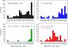 |
Fig. 1 Spectral type distributions for the O-type stars. The whole sample is shown in the upper left panel in black. The remaining panels show the spectral type distribution for the luminosity subclasses within the sample: O V stars in blue, O IV, O III–IV, and O V–III in green, O Vz in red (and O Vz? by the grey hatched areas). |
2. Sample selection
For this study we selected the apparently single unevolved O-type stars identified by Sana et al. (2013) and Walborn et al. (2014) that have sufficiently good spectra for reliable quantitative analysis. Walborn et al. (2014) divided the 340 O-type stars in the VFTS into two groups, “AAA” and “BBB”, comprising 213 and 127 stars, respectively. The BBB group were spectra rated as lower quality as a result of problems such as low signal-to-noise ratio, strong nebular contamination, double-lined binaries, and difficulties in precise classification. The BBB stars were excluded from our sample, as were AAA stars identified by Sana et al. (2013) as single-lined binaries (i.e. those for which radial-velocity variations of > 20 km s-1 were detected). This led to a sample of 105 stars with luminosity classes V and IV (including the Vz subclass, the uncertain classification V–III, and III–IV, which indicates a precise interpolation between III and IV), as listed in Tables A.1 and A.2 (with a complete description of the information in the tables given in Sect. 4). Although we describe these stars as apparently single objects, we note that some spectra probably include the contribution of more than one star (which may not necessarily be physically bound, see Sect. 3).
The distribution of spectral types of our sample is shown in Fig. 1. The sample is concentrated at medium and late types, with peaks at O6 and O9.5, with only seven stars earlier than O4. Interestingly, different distributions are found when the stars are separated by luminosity class. Contrary to the distribution of the “normal” O V stars, which are concentrated mainly at spectral types later than O8, the distribution of O Vz stars dominates at medium subtypes; we refer to Paper XIII for a detailed discussion of the origin of this bimodal distribution of O V and O Vz stars. Only a few O IV stars are in the sample, and these are mostly O9.5 objects. For completeness, the location of the various subgroups of our sample in the 30 Dor region is shown in Fig. 2.
 |
Fig. 2 Spatial distribution of our sample stars in 30 Dor. Luminosity subclasses are indicated as follows: blue circles for O V stars, red triangles for O Vz stars (including those with doubtful V/Vz classifications), and green squares for O IV stars (including V–III and III–IV classes). The central and southwestern orange circles (with adopted radii of 2.́4, see e.g. Sana et al. 2013) indicate the approximate extent of NGC 2070 and NGC 2060, respectively. |
3. Observations
The VFTS observations were obtained at the Very Large Telescope (VLT) at Paranal in Chile, using the Fibre Large Array Multi-Element Spectrograph instrument (FLAMES; Pasquini et al. 2002). Details of the VFTS observations and data were given by Evans et al. (2011).
We employed the same data as those used by Ramírez-Agudelo et al. (2013), Walborn et al. (2014), and Sabín-Sanjulián et al. (2014). These comprise spectra obtained using the fibre-fed Medusa mode of FLAMES and three of the standard settings of the Giraffe spectrograph2: LR02, LR03, and HR15N (see Table 1). As described by Evans et al. (2011), the VFTS gathered multi-epoch observations of all stars in the survey. Details regarding the combination of the multi-epoch LR02 and LR03 data to produce the final spectra discussed were given by Walborn et al. (2014).
Spectral coverage and resolving power (R) of each setting in the FLAMES–Medusa mode used by the VFTS.
Figure 3 shows six representative examples of Medusa spectra from our sample, covering the different luminosity classes (IV, III–IV, V–III, V, and Vz). As described in Paper XIII, the observed spectral range includes H i and He i/ii lines (plus several N iii/iv/v lines, see Sect. 4) suited to determine the important physical parameters of O-type stars. We also note the presence of nebular emission lines in most of the spectra.
Absolute magnitudes (Col. 5 in Tables B.1 and B.2) were calculated using the ground-based B- and V-band photometry from Evans et al. (2011), adopting a distance modulus of 18.5 mag (e.g. Gibson 2000), and using the Bayesian code chorizos (Maíz Apellániz 2004) to take the line-of-sight extinction into account; a complete description of the method and model spectral energy distributions used (calculated for the metallicity of the LMC) was given by Maíz Apellániz et al. (2014).
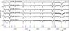 |
Fig. 3 Example O-type dwarf spectra for the range of luminosity subclasses in our sample (IV, III–IV, V–III, V, and Vz); the diagnostic H and He lines are indicated. The uppermost spectrum (VFTS 096) suffers from stellar contamination in the Medusa fibre (see Fig. 4 and Sect. 4.3.1). |
Lastly, we had access to a series of I-band images obtained with the Hubble Space Telescope (HST)3, which includes more than 80% of the stars in the VFTS. These images were helpful to investigate possible multiple sources within the Medusa fibres (see Fig. 4 for examples, and also Sabbi et al. 2012, 2016), allowing detection of composite spectra that are otherwise undetected from radial-velocity measurements, and/or stars with contaminated photometry in the ground-based imaging. For completeness, details of possible or confirmed contamination (provided by Walborn et al. 2014) are included in the final column of Tables A.1 and A.2.
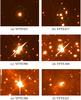 |
Fig. 4 Example HST/WFC3 images of O dwarf stars in the VFTS. The aperture of the Medusa fibres (1.̋2) is indicated by the inner green circles; the outer circles have twice this diameter to help guide the eye. VFTS 021 is shown as an example of a uncontaminated Medusa fibre, while the spectra of the others shown here are expected to have some degree of contamination from close-by companions. |
4. Stellar and wind parameter determination
4.1. Spectroscopic parameters
4.1.1. HHe analysis
Stellar and wind parameters were determined using the IACOB grid-based automatic tool (iacob-gbat, see Simón-Díaz et al. 2011). This tool is based on standard techniques for the quantitative spectroscopic analysis of O stars (see e.g. Herrero et al. 1992, 2002; Repolust et al. 2004) and has been automated by applying a χ2 algorithm to a large grid4 of synthetic spectra computed using fastwind (Santolaya-Rey et al. 1997; Puls et al. 2005; Rivero González et al. 2012a). The grid comprises ~180 000 atmosphere models, covering a wide range of stellar and wind parameters, and is optimised for the analysis of O-type stars (see also Lefever et al. 2007; Castro et al. 2012, for similar approaches using fastwind).
We followed the same strategy and criteria as were used in analysis of the O Vz subsample presented in Paper XIII. In brief, we used the grid of fastwind models computed for the metallicity of the LMC (Z = 0.5 Z⊙, see e.g. Mokiem et al. 2007a). The parameter ranges of the fastwind grid and the hydrogen and helium lines used in the analysis are shown in Tables 2 and 3 of Paper XIII. We adopted the projected rotational velocities (v sin i) from Ramírez-Agudelo et al. (2013), except for 17 stars where the global broadening of the synthetic and the observed lines did not agree; for these stars the v sin i values were iterated on until achieving a good fit. Although macroturbulent broadening of the line profiles appears to be a relatively ubiquitous feature of O-type stars (see e.g. Simón-Díaz et al. 2017), we do not expect this to be a significant factor in the context of the physical parameters studied here with H i and He i/ii, and do not include its effects separately in our line-broadening convolution. Lastly, we fixed the microturbulence and the β-parameter (i.e., the exponent of the wind velocity-law) to 5 km s-1 and 0.8, respectively, as these two parameters could not be properly constrained with the current sample (see Sects. 3.4.1 and 3.4.2 of Paper XIII).
Results from the iacob-gbat analysis of our sample (except for the targets discussed in Sect. 4.1.2) are presented in Table A.1. The column entries are as follows: (1) VFTS identifier; (2) spectral classification from Walborn et al. (2014); (3) v sin i considered in the analysis; (4–11) derived effective temperature (Teff), gravity (log g), rotation-corrected gravity5 (log gc), helium abundance6 (Y(He)), and wind-strength Q-parameter (see Sect. 6.3), and their formal uncertainties; (12) estimated values for the wind momentum Dmom (also Sect. 6.3); (13) comments from Walborn et al. regarding possible binarity or multiplicity.
We adopted a minimum value of 0.1 dex for the formal errors on log g as we consider that uncertainties below this value are not realistic. We note that several sources of uncertainty need to be taken into account besides those arising from the spectral fitting. These include the continuum renormalisation and the sampling of the fastwind grid. For the same reasons, the uncertainties in Y(He) were set to 0.02 since the errors estimated by the iacob-gbat were unrealistically low (see e.g. Herrero et al. 1992, 2002; Repolust et al. 2004). Other points to be taken into account when interpreting results from the analysis are discussed in Sect. 4.3.
4.1.2. HHeN analysis
In 20 cases the HHe analysis using the iacob-gbat failed to provide reliable results, as indicated by the broad χ2 – Teff distributions (with widths in excess of 5000 K) and/or unexpectedly low temperatures for the spectral type. After careful inspection of all the cases, we found that this was mainly due to a lack of reliable He i diagnostic lines (because of strong nebular contamination or very high temperatures). In these cases, we turned to the N ionisation balance, following the guidelines from Rivero González et al. (2011, 2012a,b).
The grids of fastwind models for different metallicities incorporated in the iacob-gbat have recently been extended to include nitrogen as an explicit model atom; however, the nitrogen lines are not yet included in the iacob-gbat computations. A detailed HHeN analysis of the complete O-dwarf sample (also including N abundances) is now in progress and will be presented in a forthcoming paper (Simón-Díaz et al., in prep.). For the purposes of the current study we performed a traditional by-eye HHeN analysis of the 20 stars for which the automated HHe analysis did not provide reliable results. In these analyses we fixed the helium abundance to Y(He) = 0.10, considered the parameters associated with the best-fitting model, and adopted the following formal errors for Teff, log g, Y(He), and log Q: 1500 K, 0.10 dex, 0.02, and 0.20, respectively. The results for these 20 stars are summarised in Table A.2 (which includes the same information as Table A.1, but for quantities fixed in the analysis).
4.2. Radii, luminosities, and masses
Stellar radii, luminosities, and spectroscopic masses were calculated following the relations described by Kudritzki (1980), which connect the absolute magnitude in the V band and the stellar radius (see also Herrero et al. 1992; Repolust et al. 2004).
Evolutionary masses (Mev) were estimated in the classical way, that is, by interpolating between evolutionary tracks by Brott et al. (2011) in the H–R (log L/L⊙ vs. log Teff) and Kiel (log gc vs. log Teff) diagrams.
We also used the Bayesian bonnsai tool7 (Schneider et al. 2014). In contrast to more traditional approaches, bonnsai simultaneously accounts for all available observables (i.e. log L/L⊙, log gc, Teff, v sin i) and, assuming prior knowledge of the initial mass function, for example, it computes full posterior probability distributions of the various stellar parameters for a given set of evolutionary models. For our sample we used bonnsai to match the derived luminosities, effective temperatures, surface gravities, and projected rotational velocities to the evolutionary models of Brott et al. (2011) and Köhler et al. (2015). We assumed a Salpeter initial mass function (Salpeter 1955) as the initial-mass prior, adopted the distribution of rotational velocities of O-type stars in 30 Dor from Ramírez-Agudelo et al. (2013) as the initial rotational velocity prior (and assuming that their rotational axes are randomly orientated in space), and adopted a uniform prior for stellar ages. Tables B.1 and B.2 summarise this second set of stellar parameters, in which the column entries are (1) VFTS identifier; (2) spectral classification; (3) effective temperature; (4) rotation-corrected gravity; (5) absolute visual magnitude MV; (6–11) radii, luminosities, and spectroscopic masses and their corresponding formal errors; (12, 13) evolutionary masses calculated from the Kiel diagram, using evolutionary tracks with an initial rotational velocity of 171 km s-1 (see Sect. 6.1) and their corresponding errors; (14, 15) the same as (12, 13), but using the H–R diagram; and (16) evolutionary masses derived using bonnsai and their errors.
4.3. Cautionary remarks
During the analysis of our sample we found various cases for which we could only provide upper or lower limits. We also detected a few stars for which a quantitative spectroscopic analysis based exclusively on the H and He lines could not provide reliable estimates of the effective temperature (see Sect. 4.1.2). A summary of the number of stars with problematic analyses is shown in Table 2.
Number of stars in our analysis with problematic χ2 distributions of wind strength (log Q), effective temperature (Teff), helium abundance (Y(He)), and surface gravity (log g) caused by degeneracies or because they reach the boundaries of the grid.
4.3.1. Stellar contamination in the fibre aperture
Known spectroscopic binaries were omitted from our sample, but as illustrated in Fig. 4, some of the VFTS spectra are contaminated by light from nearby companions on the sky (which are not necessarily in bound binary or multiple systems). We therefore need to consider the effect of this on the parameters estimated by our analysis (Teff, log g, Y(He), etc.) and/or the parameters inferred from potentially erroneous absolute magnitudes (R,L,M).
When a certain shift between both components is present, Balmer lines may appear too broadened and therefore a higher surface gravity will be derived, which also affects Teff. Additionally, the dilution effect in a composite spectrum could weaken the He lines, thus leading to lower helium abundances.
The spectroscopic mass (Msp) depends on the stellar radius. When the photometry of the target star is contaminated by a nearby companion, the derived radii can therefore be overestimated by up to ~35% (in the worst-case scenario of two equally bright components), leading to an overestimate of Msp of ~70%. Similarly, such contamination in the fibre would also lead to overestimated evolutionary masses through a higher inferred luminosity, which moves the star to higher masses in the H–R diagram.
4.3.2. Nebular contamination in the fibre aperture
Extreme cases of nebular contamination were omitted from our sample by excluding the BBB stars from Walborn et al. (2014). Still, ~70% of the spectra in our sample display relatively strong nebular contamination in Hα and some degree of contamination in the He i lines. This may affect the determination of stellar parameters and must be handled with care. The most critical parameters that can be affected are Teff and log Q because the He ionisation balance and Hα line are the main diagnostics for these parameters, respectively; log g and Y(He) may also be affected to a lesser extent.
We checked each case individually and found that the situation is not critical for most stars and only results in larger uncertainties. However, in 11 objects (with spectral types later than O4) the He i lines should be sufficiently strong to be used in the HHe analysis, but a strong nebular contamination rendered them unusable. These cases were therefore analysed using HHeN diagnostics (see Sect. 4.1.2, with results given in Table A.2).
4.3.3. Earliest spectral types
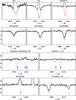 |
Fig. 5 Model fits to the spectrum of VFTS 621, with the best fit from the HHe (Teff = 36 kK, log g = 3.8) and HHeN (Teff = 54 kK, log g = 4.2) analyses shown in red and blue, respectively. The log Q as well as the helium and nitrogen abundances are the same in both models. These single-star models both suffer deficiencies that are suggestive of a composite observed spectrum, as seen in HST images (Fig. 4). |
For nine stars with spectral types earlier than O4, the He i lines were too weak or even nonexistent (e.g. VFTS 072). The χ2 distribution for Teff for these stars showed degeneracies, therefore we resorted to analysing them using the nitrogen lines described in Sect. 4.1.2. Results for these stars are presented in Table A.2.
In the course of this analysis we noted that He i lines are present in the spectra of VFTS 468, 506 and 621, which is unexpected given their classification as O2 type. This qualitative (morphological) argument is reinforced by the results of our HHeN analysis. Inclusion of the diagnostic N iii/iv/v lines confirmed our suspicion that the HHe analysis returned estimates of Teff (and hence log g) that were too low, but the best-fitting HHeN models do not predict He i intensities as strong as in the data (particularly for He i λ4471).
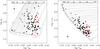 |
Fig. 6 Kiel (left) and H–R (right) diagrams for our sample. Class V objects are plotted in black, those with other luminosity classes (IV, III–IV, and V–III) in red. Stars analysed using HHeN lines are plotted as diamonds, while those with (stellar) contamination in the fibre aperture (see Sect. 4.3.1) are plotted as open symbols. Evolutionary tracks and isochrones for the LMC are from Brott et al. (2011) and Köhler et al. (2015), with an initial rotational velocity of 171 km s-1 (see Sect. 6.1). The zero-age main-sequence (ZAMS) is indicated in the two plots by the bold black line, and typical uncertainties are indicated in the upper and lower corner, respectively. |
In these three cases we also noted that the broadening required to fit the observed He i lines is much larger than the broadening needed to fit the nitrogen lines. An example of this is shown Fig. 5, where the best-fitting HHe and HHeN models for VFTS 621 are shown in red and blue, respectively. The HHe fit predicts N iv/v lines that are too weak (or nonexistent) and N iii absorption that is too strong, while the HHeN model predicts He iλ4471 absorption that is too weak, together with He ii lines that are too strong.
These inconsistencies could be related to multiplicity and/or nitrogen peculiarities: VFTS 621 was noted by Walborn et al. (2014) as a visual multiple with three components (VM3, see also Walborn et al. 2002b), VFTS 468 is classified as O2 V((f*)) + OB and noted as a visual multiple with four components (Walborn et al. 2014), and VFTS 506 is classified as an ON2 star (and classified as a (small-amplitude) single-lined binary by Sana et al. 2013). These examples of probably composite spectra appear similar to the case of Sk 183 in the Small Magellanic Cloud (Evans et al. 2012). Sk 183 was initially classified as an O3 dwarf according to its nitrogen lines, but He absorption in its spectrum suggested a later type. Spectral analysis by Evans et al. (2012) found that the He i and He ii lines could not be fitted simultaneously using a single model, and that better fits could be achieved using a composite (O + B) model. Similar inconsistencies were also noted by Rivero González et al. (2012b,a) in their HHeN analysis of O-type stars in the Magellanic Clouds. Particularly for their ON2-type giants, they failed to simultaneously fit the observed He i λ 4471 and nitrogen lines using both the fastwind and cmfgen (Hillier & Miller 1998) codes.
These three O2-type stars show the importance of including information on possible close-by companions (that are not necessarily physically bound) to elucidate the difficulties found in the analysis of some stars, and the apparent bimodality found in the literature for the derived Teff at the earliest spectral types (see Sect. 5.2). In this context of interpreting ground-based spectroscopy, an increasingly important input is results from surveys of massive stars at high spatial resolution (e.g. Mason et al. 1998, 2009; Sabbi et al. 2012, 2016; Sana et al. 2014; Aldoretta et al. 2015). Also promising is the use of spatially resolved spectroscopy to separate different components (Walborn et al. 1999, 2002a; Sota et al. 2011). The fourth O2 star in our sample, VFTS 072, appears to be a simpler case as no He iλ4471 is present. The derived temperature is higher when including the nitrogen lines, but no signatures of a companion are present in the spectrum. Unfortunately, we do not have the corresponding HST image to investigate if this star appears genuinely isolated.
4.3.4. Thin winds
As we discussed in Paper XIII, for some stars we encountered degeneracies in the χ2 distributions of log Q due to weak winds, which render the Hα and He ii λ4686 lines insensitive to changes in this wind parameter. For ~66% of the sample we were therefore only able to provide upper limits for log Q (see Col. 10 in Table A.1).
4.3.5. Helium and gravity
We found 14 cases (4 O Vz, 9 O V, and 1 O IV) for which we could provide only upper limits for the helium abundance (see Col. 9 in Table A.1), and 10 cases (5 with low He abundance as well) with log g > 4.2 (marked with asterisks in Col. 6 of Table A.1) that are relatively high compared to predictions by theoretical evolutionary models. These features could indicate binarity (see Sect. 4.3.1), which would affect the position of these stars in the Kiel or H–R diagrams, thus modifying the estimated spectroscopic and evolutionary masses.
5. General properties of the sample
5.1. Stars in the Kiel and H–R diagrams
To investigate the evolutionary state of our sample of stars, we plot them in the Kiel (log gc – log Teff) and H–R diagrams, as shown in Fig. 6 (in which we have highlighted the different luminosity classes)8. Evolutionary tracks and isochrones by Köhler et al. (2015) and Brott et al. (2011) for an LMC-like metallicity are shown.
We remark that a reliable determination of effective temperatures is critical when studying the position of the stars with the earliest spectral types in the H–R and Kiel diagrams, as this has a direct effect on the determination of their evolutionary masses and luminosities. For example, the inferred evolutionary masses can range from 70 M⊙ to 150 M⊙ for effective temperatures spanning 50 000 K to 55 000 K. Because of this and the apparently composite nature of three of our O2-type stars (see Sect. 4.3.3), we treat them with particular care in the following sections.
5.1.1. Kiel diagram
The rotation-corrected gravities of our sample mostly span 3.8 < log gc < 4.2. We note that relatively few stars lie below the 1 Myr isochrone, which might be a consequence of the fastwind/cmfgen discrepancy noted by Massey et al. (2013). These authors found that gravities derived with cmfgen were typically 0.1 dex higher than those obtained using fastwind. We are therefore careful when considering masses inferred from the Kiel diagram, denoting the evolutionary state “in terms of gravity”. That said, we note that if the difference between the codes were the sole cause, then results from cmfgen would be expected to place at least six stars below the zero-age main-sequence (ZAMS).
Except for the O2 stars, our Kiel diagram has a dearth of objects close to the theoretical ZAMS for masses above ~35 M⊙. A similar result was found by Castro et al. (2014) for a sample of 575 Galactic OB stars. The authors pointed out that such stars could still be embedded in their birth clouds, which would hamper their detection at optical wavelengths (Yorke 1986). Alternatively, if this absence of stars with masses above ~35 M⊙ were real, this empirical result may present an important challenge to theories of massive-star formation.
The class IV stars are mostly concentrated at log Teff ≲ 4.55, with 3.8 < log gc < 4.0. As the intermediate class between dwarfs and giants, the O IV stars are expected to be more distant from the ZAMS (in terms of gravity) than the class V objects. Most of the class IV stars define an upper envelope in gravity for stars with 4.52 < log Teff < 4.55, confirming the expectation of a slightly more evolved state (in terms of their gravities). However, there are three stars (VFTS 303, 505, and 710) with 4.53 < log Teff < 4.55 with gravities that appear too high (log gc > 4.2) for their luminosity class. Possible binarity or composite spectra could explain these results: either by confirmed (VFTS 303) or possible (VFTS 505) contamination in the fibre aperture, or suspected spectroscopic binarity (VFTS 710). We highlight that Ramírez-Agudelo (2017) have found similar cases in their analysis of the giants and supergiants from the VFTS, where several late-type class II and III stars have estimated gravities of log g = 4.0 to 4.5 (more in line with those expected of dwarfs). Intricacies in the luminosity classification may have played a role in these cases, where the Si iv absorption is weaker than expected for giants, pointing to a dwarf or subgiant classification rather than a giant classification (see also Walborn et al. 2014).
5.1.2. H–R diagram
As shown in Fig. 6, most of our sample have luminosities ranging between log L/L⊙ = 4.5 and 5.7. Most of the O IV stars have luminosities in the range ~4.5 < log L/L⊙ < 5.1, with inferred ages of ~3–5 Myr, somewhat more evolved than the dwarf subsample, as expected. As in the Kiel diagram, VFTS 505 and 710 appear to be too young (on or below the ZAMS), although VFTS 303 is located within the main group of class IV stars. Interestingly, a larger number of stars are located between the ZAMS and the 1 Myr isochrone in the H–R diagram, which is less affected by the possible underestimation of the gravities discussed above.
 |
Fig. 7 Estimated effective temperatures (Teff) and rotation-corrected gravities (log gc) for our sample as a function of spectral subtype (using the same symbols as in Fig. 6); small shifts have been added to the abscissae of each star to avoid overlap. The upper panel shows the number of stars per subtype. |
5.2. Spectral calibrations
Spectral calibrations are useful tools to characterise the physical properties of massive stars, with applications in several astrophysical fields, such as studies of H ii regions and population synthesis. As the largest sample to date (and with complete coverage of spectral types), the VFTS results offer a unique opportunity to characterise the Teff scale of O dwarfs in the LMC.
5.2.1. Teff and log g calibrations
To construct calibrations from our sample, we plot the Teff and log gc estimates in Fig. 7 as a function of spectral subtype, including results from both the HHe and HHeN analyses (plotted as circles and diamonds, respectively, and red symbols for stars with luminosity classes IV, III-IV, and V-III). Our sample covers the whole range of O subtypes, from O2 to O9.7, but has two peaks (at O6 and O9.5) and is dominated by stars with types of O6 or later. Moreover, we only have one object for each subtype from O2.5 to O3.5.
The effective temperature decreases from ~55 000 K for O2 stars to ~34 000 K by O9.7. There is a linear trend between O2.5 and O9.7, even taking into account the stars analysed with HHeN lines (diamonds in the figure), but the four O2-type stars seem to break this trend.
There is a notable dispersion in Teff and log g for almost every spectral subtype. This effect was discussed by Simón-Díaz et al. (2014), who compared the Teff and log g scales for populations of O dwarfs in the Galaxy (analysed within the IACOB project, see Simón-Díaz & Herrero 2014) and the results for the LMC stars presented in Paper XIII (which are also included in the current study). Simón-Díaz et al. warned against the use of spectral calibrations based on small samples of O-type dwarfs, as a relatively evolved O dwarf population is expected to show a wide range of gravities because of the different evolution of early- and late-type O dwarfs.
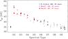 |
Fig. 8 Effective-temperature scale for our sample of stars (in grey) compared with results from Rivero González et al. (2011, 2012b,a), Mokiem et al. (2007a), and Massey et al. (2005). |
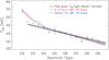 |
Fig. 9 Comparison of our Teff calibration for O dwarfs in the LMC with those derived by Rivero González et al. (2012a,b) and adopted by Doran et al. (2013). Grey dots and bars represent the mean value and standard deviation of our Teff estimates for each spectral type, with our linear fit shown by the black line (and the grey zones indicating the associated uncertainties). |
5.2.2. Comparison with Rivero González et al.
The most complete Teff calibration for LMC O-type stars before this study is the work of Rivero González et al. (2012a,b), who used HHeN diagnostics to analyse optical spectroscopy of 25 stars (including 16 dwarfs); our temperatures are compared to their results in Fig. 8, with generally good agreement between the two distributions. There is one star in common between the two studies, namely VFTS 072 (= BI 253). We obtain a similar temperature (Teff = 54 000 K vs. their estimate of 54 800 K), while our gravity is slightly lower (log g = 4.00 vs. 4.18). When we compare the spectra, a small difference in the wings of the Balmer lines in the 4000–5000 Å range is visible (likely an artefact of the continuum normalisation, although we note that the Hα profiles are very similar), which most likely relates to differences in spectral resolution (the “older” data were obtained at R = 40 000) and different levels of nebular contamination in the line cores (fibres vs. slit spectroscopy).
For a more quantitative comparison, a linear fit to our data (excluding the O2 stars) is given by ![Mathematical equation: \begin{equation} T_{\rm{eff}}\,[{\rm kK}] = 49.75(\pm 0.54) - 1.64(\pm 0.07) \times {\rm SpT}, \end{equation}](/articles/aa/full_html/2017/05/aa29210-16/aa29210-16-eq30.png) (1)where SpT is the number corresponding to the spectral subtype. This calibration is shown in Fig. 9, compared to the fit from Rivero González et al., who divided their calibration into quadratic and linear components for spectral types earlier and later than O4, respectively. We find excellent agreement between both scales for types later than O4, while Teff values for O2.5-O4 stars are slightly hotter than our fit (albeit lower than their quadratic fit), and our results for the O2 stars agree with their calibration.
(1)where SpT is the number corresponding to the spectral subtype. This calibration is shown in Fig. 9, compared to the fit from Rivero González et al., who divided their calibration into quadratic and linear components for spectral types earlier and later than O4, respectively. We find excellent agreement between both scales for types later than O4, while Teff values for O2.5-O4 stars are slightly hotter than our fit (albeit lower than their quadratic fit), and our results for the O2 stars agree with their calibration.
As commented above, the small number of stars observed at the earliest types, in combination with the intrinsic scatter of a Teff – SpT calibration and difficulties of both the observations and analysis, do not allow us to reach a firm conclusion on the need for a change in slope of the calibration in the O2.5-O4 range. A larger sample of early O-type stars, including information on the possible binary or composite nature of their spectra, is needed to shed more light on the temperature scale. This should be possible using data from a recent HST program by Crowther et al. (2016) to obtain ultraviolet and optical spectroscopy of the massive stars in R136, the central cluster of 30 Dor. There are a large number of O2-3 V stars in R136, and analysis of their optical spectroscopy from HST should provide a firmer understanding of the temperatures at the earliest spectral types.
5.2.3. Comparison with other calibrations
There are other results in the literature for O dwarfs in the LMC, although they do not have such thorough coverage in terms of spectral type. Massey et al. (2004, 2005, 2009) performed HHe fastwind analyses of optical spectra from 19 stars (9 O V) in the LMC, together with 35 stars in the Milky Way and Small Magellanic Cloud (SMC). Results from Massey et al. for LMC dwarfs are shown in red in Fig. 8. These were limited to spectral types earlier than O5, and include three stars with uncertain classifications of O2-3.5 V and one O2 star with only a lower limit on its temperature (due to the absence of He i lines); these four stars are plotted with open symbols in the figure. The results from Massey et al. are generally consistent with our distribution (given the uncertainties in classification for some of their stars). The authors found lower temperatures and gravities for the two O2 stars in their sample, but this could be related to the effects discussed above in Sect. 4.3.3.
In Fig. 8 we also include the results from a HHe analysis with fastwind of 13 dwarfs in the LMC (spanning O2 to O9.5 types) by Mokiem et al. (2007a). Again, subject to problems for the O2-type stars with only a HHe analysis, their results agree reasonably well with ours.
Doran et al. (2013) adopted a Teff scale for the O dwarfs in 30 Dor based on the calibration from Martins et al. (2005), revised upwards by 1000 K to adapt it for the metallicity of the LMC. For spectral types earlier than O3.5, they used individual estimates from Rivero González et al. (2012a) and Doran & Crowther (2011). The scale from Doran et al. is practically identical to that from Rivero González et al. (2012a), with the exception of the O3.5 stars (with the former ~1400 K hotter), as shown in Fig. 9.
Lastly, we note that eight of our O-type dwarfs9 from the HHeN analysis overlap with the VFTS sample analysed using cmfgen by Bestenlehner et al. (2014) to understand the wind properties of the luminous O and Wolf–Rayet stars. The estimated temperatures and luminosities from Bestenlehner et al. are in reasonable agreement for the four stars later than O2 (with differences of ΔTeff ~ 1000 K and Δlog L/L⊙ ~ 0.01, i.e. compatible within the estimated uncertainties). For the four O2-type stars (VFTS 072, 468, 506, and 621) we obtain effective temperatures up to ~14% higher, with luminosities of 1 to 3% higher. However, as their main objective was to investigate the wind properties, Bestenlehner et al. adopted log g = 4.0 in their analyses, which affects the ionisation equilibrium and might explain the differences in Teff for VFTS 468, 506 and 621, for which we derive log g = 4.2. The composite nature of the spectra discussed in Sect. 4.3.3 and the different analysis methods probably also contribute to the different Teff estimates.
6. Discussion
6.1. Rotation and helium abundance in an evolutionary context
6.1.1. v sin i distribution
The v sin i distribution for our O dwarfs is presented in Fig. 10. It peaks in the 40–80 km s-1 bin, with most stars found at v sin i ≲ 150 km s-1. Given the limitations of the strategy applied to determine v sin i in the O-type sample (see Ramírez-Agudelo et al. 2013), the first two bins in Fig. 10 must be considered with care. Given the lack of useful metal lines in the observed spectral range, using He i lines (or even He ii in some critical cases) to estimate v sin i, combined with the presence of nebular contamination and/or low signal-to-noise ratio, leads to large relative uncertainties in estimates below ~100 km s-1.
The tail of the distribution extends to high rotational velocities. The star at ~600 km s-1 is VFTS 285, one of the fastest rotators known to date (see Walborn et al. 2012, 2014). We find a low but noteworthy peak over the 240–440 km s-1 range (see also Ramírez-Agudelo et al. 2013), which could originate from the effects of mergers and mass transfer (via Roche-lobe overflow) in binary evolution (de Mink et al. 2013, 2014).
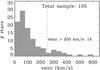 |
Fig. 10 Projected rotational velocities for our sample of O-type dwarfs. Fourteen stars have v sin i > 250 km s-1 (with the velocity threshold indicated by the vertical dashed line). |
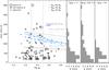 |
Fig. 11 Left: projected rotational velocities (v sin i) vs. rotation-corrected gravities (log gc) for our sample, grouped according to helium abundance. Theoretical predictions for the LMC from Brott et al. (2011) are shown in grey (for three initial masses and two initial rotational velocities as indicated). Predictions for solar metallicity and an initial vini of 40% the critical velocity from Ekström et al. (2012) are shown in blue. Right: v sin i distributions for three ranges of gravity: (1) low (log gc < 3.9); (2) intermediate (3.9 ≤ log gc ≤ 4.1); and (3) high (log gc > 4.1). |
6.1.2. Rotation vs. gravity
Our projected rotational velocities were investigated as a function of rotation-corrected gravity, as shown in Fig. 11. Overlaid on the figure are theoretical predictions from Brott et al. (2011) for three initial stellar masses (20, 30 and 40 M⊙) and two initial rotational velocities (171 and 337 km s-1).
The distribution of stars in Fig. 11 can be roughly separated into three groups when compared with the evolutionary tracks. Firstly, most of the stars of the sample are found at lower velocities than the vini = 171 km s-1 tracks. Taking into account that the v sin i values are lower limits on vrot due to projection effects, the use of models with vini = 171 km s-1 to study our sample in an evolutionary context seems a reasonable approach. Secondly, evolutionary tracks with vini = 337 km s-1 can explain the stars above the 171 km s-1 tracks, which includes most of the fast rotators. Finally, there is a third group of extremely rapid rotators, above the vini = 337 km s-1 track – it is unclear if these were born with such rapid rotational velocities or if they are the products of binary evolution. Estimates of nitrogen abundances and proper motions may help clarify their nature.
In the right-hand panels of Fig. 11 we show the v sin i distribution for three ranges in log gc (>4.1, [4.1, 3.9] and <3.9). The rapid rotators seem to be more frequent at intermediate gravities, less common at higher values (i.e. younger), and absent at log gc < 3.9 (older). We performed a Kuiper test (Kuiper 1960) to see if this possible evolution in the v sin i distributions was statistically significant. In general terms, the Kuiper test compares the cumulative distributions of two data samples to estimate if they can be drawn from the same parent distribution. Importantly, the test is sensitive to the extremes of the distribution, where we find our fast rotators. For the test, we denoted the three distributions in the right-hand panel of Fig. 11 as “1”–“3” (from left to right). From applying the Kuiper test, distributions 1 and 2 have a probability of 94% of being derived from the same parent distribution, whereas distributions 2 and 3 only have a 6% probability to be drawn from the same parent sample.
The evolutionary models (for LMC metallicity) from Brott et al. (2011) predict that rotation remains constant down to log gc ~ 3.5, which appears somewhat incompatible with the trend above. In Fig. 11 we also include evolutionary tracks from the Geneva group (Ekström et al. 2012, for Solar metallicity). Their models predict a decrease in rotational velocity from ~300 to ~200 km s-1, which is still not sufficient to explain the observed behaviour. As a word of caution we recall that the evolutionary models we compare with here solve for the stellar structure in one dimension. They do not show the possible variations in effective surface gravity with latitude, which may be important in stars that rotate at a significant fraction of their break-up rate. These results may imply that the angular momentum transport is not properly taken into account in current evolutionary models and that braking should be more efficient at earlier ages. Whether this braking is related to mass loss at the surface, magnetic fields, or other physical processes cannot be assessed with the current data.
6.1.3. Rotation in the Kiel and H–R diagrams
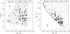 |
Fig. 12 Kiel (left) and H–R (right) diagrams for our sample grouped according to v sin i. Black filled circles: v sin i < 250 km s-1; red open circles: v sin i ≥ 250 km s-1. Evolutionary tracks and isochrones for an initial v sin i = 171 km s-1 from Brott et al. (2011) are also shown. |
Further Kiel and H–R diagrams for our sample stars are shown in Fig. 12, where our sample is now grouped by v sin i (lower and higher than 250 km s-1, plotted as black and red circles, respectively). Stars with v sin i < 250 km s-1 do not appear to have a particular pattern in the H–R diagram, but those with more rapid rotation appear to be mostly concentrated at M < 30 M⊙ and closer to the ZAMS compared to the rest of the sample. As indicated by Walborn et al. (2014), most of the rapid rotators are located outside the main clusters in 30 Dor (NGC 2060 and NGC 2070), which may indicate a runaway nature, a binary formation scenario, or both (Packet 1981; Langer et al. 2008; Walborn et al. 2014; Platais et al. 2015). Future analyses with HST imaging and nitrogen abundances (Simón-Díaz et al. in prep., Grin et al. 2017) will help constrain the origin of these extremely rapid rotators, providing ideal targets to refine our understanding of rotational-mixing processes, chemical evolution, and binary interaction (see, e.g. Hunter et al. 2008).
The fastest rotators (above the v sin i = 337 km s-1 tracks in Fig. 11) have Mev < 25 M⊙, and some even below 20 M⊙ (see Table B.1). From the Kiel diagram in Fig. 12, a star with an initial mass of 20 M⊙, will have Teff ~ 30 000 K when reaching log gc = 3.9. With these properties the star would be classified as an O-giant or even a B star, and thus outside our O-dwarf sample. Indeed, the stars with log gc < 3.9 in Fig. 11, are mostly class IV, III–IV, and V–III objects.
In view of this result, we were concerned that the drop of v sin i at relatively low gravities (see Sect. 6.1.2) might arise from stars with initial masses below 25 M⊙ but that will no longer be classified as O-type dwarfs once they reach log gc < 3.9, particularly at large v sin i. To check this we included provisional results for stars with initial masses higher than 15 M⊙ that have evolved into O and B giants (Ramírez-Agudelo 2017; Schneider et al., in prep.). A Kuiper test of the updated distributions for groups 2 and 3 found that the probability to be drawn from the same parent distribution is still ~10%. This preliminary test indicates that this possible bias can probably not explain the lack of fast rotators below log gc ~ 3.9, although we remark that the parameters for some stars still have to be confirmed, and we will revisit this in a future study.
6.1.4. Helium abundances
Helium abundances for our sample were also indicated in Fig. 11. Most of our stars have Y(He) < 0.12, i.e. normal abundances within the estimated uncertainties. There were 14 stars for which we could not obtain good determinations of Y(He), and where only upper limits of ~0.08 could be estimated (with the best-fitting models being 0.06 or less). As explained in Paper XIII, these low abundances could be a consequence of undetected binarity, the effects of low signal-to-noise ratio, and/or nebular contamination in the spectra.
We found five stars with enhanced helium abundances (Y(He) > 0.12) and log gc > 3.9. Two, VFTS 724 and VFTS 285, are rapid rotators with v sin i = 370 and 600 km s-1, respectively. The rapid rotation of these two stars could explain their high helium abundances (see e.g. Maeder 1987; Langer 1992; Denissenkov 1994; Herrero et al. 1999). The other three stars (VFTS 089, 123, and 761) have intermediate and low rotation rates. Rapid rotation might still explain the He excess of these stars given that their true rotational velocities might be higher because of projection effects. Equally, their He enhancements might indicate past mass transfer from an undetected binary (e.g. Hunter et al. 2008), and they could be magnetic stars (see e.g. Schneider et al. 2016). We note that stellar winds are unlikely to be the cause for the He enrichment, as such strong winds should generate a larger surface enhancement, with wind features also seen in the spectra.
6.2. Mass-discrepancy problem
As noted earlier, evolutionary masses (Mev) are typically estimated by placing a star in the H–R diagram (using results from spectral analysis) and interpolating between evolutionary tracks. Ideally, Mev should agree with the spectroscopic mass (Msp), calculated from Teff, log g, and R from the spectral analysis, but this is not always the case and is known as the “mass-discrepancy problem”.
This discrepancy has been a challenge in the determination of masses in O-type stars since it was identified by Herrero et al. (1992). Possible explanations have included uncertain distance estimates to Galactic stars, problems with stellar atmosphere models (e.g. underestimated gravities or the treatment of mass-loss), and problems in the evolutionary models (treatment of overshooting, rotation, and/or binary evolution). However, given a diversity of results across a range of metallicities, this issue remains unresolved (e.g. Herrero et al. 2002; Massey et al. 2005; Mokiem et al. 2007b; Weidner & Vink 2010; Morrell et al. 2014; Mahy et al. 2015), therefore we used our mass estimates to investigate if this effect is present in our sample of O dwarfs in the LMC.
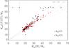 |
Fig. 13 Evolutionary masses (Mev) estimated using the H–R (Mev(LT), red crosses) and Kiel diagrams (Mev(GT), black dots) compared to those from bonnsai (Mev(B)). Error bars are shown in the upper left corner. The dashed line traces the one-to-one ratio, with differences of ±10% and 20% shown by the dotted lines. O2 stars are not included here. |
6.2.1. Best approach to estimate evolutionary mass?
Although H–R diagrams are generally used to estimate Mev, some authors prefer using the Kiel diagram, which allows a comparison of parameters obtained directly from spectroscopic analysis (thus uncontaminated by insecure distances, although less relevant in the case of the LMC). An alternative approach is provided by the Bayesian method of Schneider et al. (2014), which makes use of all the available spectroscopic parameters simultaneously (see Sect. 4.2). A further alternative is the so-called spectroscopic H–R diagram (Langer & Kudritzki 2014; Castro et al. 2014), which also only uses parameters from spectral analysis by constructing the Teff4/g ratio (which is proportional to luminosity at constant stellar mass). It was not be used here since the distance to the LMC is well constrained.
Before investigating the masses of our sample, we examined how the choice of method affected on the results. We note that O2 stars have been excluded from this study because their photometry is strongly affected (see Sect. 4.3). Figure 13 compares our Mev estimates from the H–R diagram (Mev(LT)), the Kiel diagram (Mev(GT)), and bonnsai (Mev(B)). We find reasonable agreement between Mev(LT) and Mev(B): the majority agree to within ± 20% (with 65% agreeing to <10%, and with differences of >20% for only 15 stars). In contrast, there is a non-negligible number of stars for which Mev(GT) is significantly higher (>20%) than Mev(LT) and Mev(B).
The mean and standard deviation for Mev(B) − Mev(LT) and Mev(B) − Mev(GT) are −0.6 ± 2.3 M⊙ and 2.2 ± 4.0 M⊙, respectively. When not all parameters are available, our findings therefore indicate that Mev(LT) is a better proxy for Mev(B) than Mev(GT) (both smaller dispersion and error bars). However, we conclude that all three methods give globally consistent results, in the sense that the differences will not affect investigation of the mass discrepancy. In the following, we adopt mass estimates from bonnsai because the tool makes use of all the available parameters (see Sect. 4.2), and provides valuable information on the significance of the results.
6.2.2. Evolutionary vs. spectroscopic masses
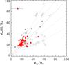 |
Fig. 14 Evolutionary-mass estimates from bonnsai (Mev(B)) vs. spectroscopic masses (Msp). Grey open symbols: possible single-lined spectroscopic binaries (Sana et al. 2013; Walborn et al. 2014), stars with poor fits to He lines, high gravities (log g > 4.2) or low helium abundance, and objects with possible or confirmed fibre contamination. Filled grey symbols: objects from HHeN analysis and no indications of binarity or fibre contamination. Red symbols: rest of the sample. The dashed grey line indicates the one-to-one relation, with ±25 and ±50% shown by the dotted lines. Typical error bars are given in the upper left corner. O2 stars were excluded. |
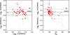 |
Fig. 15 Differences between gravities derived from bonnsai and those obtained from the spectroscopic analysis (log gc) as a function of the latter (left-hand panel) and spectroscopic mass (Msp, right-hand panel). The dashed lines mark the ±2σ region used to calculate the mean differences; symbols have the same meaning as in Fig. 14. O2 stars were excluded. |
The evolutionary masses obtained with bonnsai are compared with those obtained from the spectroscopic analysis in Fig. 14. The parameters for all stars except VFTS 303 (O9.5 IV) were reproduced by the evolutionary models in the bonnsai analysis, that is to say, the resolution and goodness-of-fit tests10 were passed at a 5% significance level. In addition, the most extreme rotators (e.g. VFTS 285) are not covered by the models from Brott et al. (2011) and Köhler et al. (2015) used by bonnsai.
Most of the results in Fig. 14 are consistent with the one-to-one relation within the uncertainties, although there is a large dispersion and there are some objects with large discrepancies. This remains the case even when ignoring the results for stars with possible or confirmed contamination in the fibre and/or binary nature (see Sect. 4.3), plotted as grey open circles in Fig. 14, which dominate the Msp>Mev region of the plot.
A trend evident in Fig. 14 is that except for a few points close to unity, Mev > Msp for stars with Msp ≤ 20M⊙, similar to results from Groenewegen et al. (1989) and Herrero et al. (1992) for Galactic stars. We refer to this as a “positive” discrepancy and explore below if it constitutes a real mass discrepancy.
As mentioned in Sect. 5.1, Massey et al. (2013) noted a difference between fastwind and cmfgen results that could affect our gravity estimates. This systematic difference would then also directly underestimate Msp by an average of ~25%. As our spectroscopic analyses were performed with fastwind, we investigated if the derived gravities are indeed too low.
We calculated the mean difference between the inferred gravities from bonnsai and those determined with fastwind (log gc), as shown in the left-hand panel of Fig. 15 as a function of the latter. We see no evidence for a trend with log gc and, after discarding stars with possible fibre contamination and/or binarity (open grey circles in the figure), and clipping out points with differences larger than 2σ, the mean difference is 0.06 ± 0.03 dex. That is, the gravities from bonnsai are, on average, 0.06 dex higher than the spectroscopic results. This is well within the quoted uncertainties, although it does not rule out a small effect of underestimated gravities using fastwind.
An underestimate of spectroscopic gravities might arise from underestimating the radiative acceleration in the photosphere in fastwind, resulting in too little gravitational acceleration. However, we find no correlation of the differences in estimated gravities with effective temperature or luminosity, as we would expect if the treatment of the radiative acceleration were incorrect. Alternatively, the difference might arise from how bonnsai obtains the gravities. bonnsai takes into account that stars spend more time near the ZAMS than far away from it (see e.g. the isochrones in Fig. 6), so that the density of evolutionary models used by bonnsai is more concentrated towards higher gravities and is therefore expected to provide higher log g values.
A general shift of all fastwind gravities would not solve the situation in Fig. 14. The estimates of Msp would increase by about 11%, which would not help much at Msp ≥ 20 M⊙. This is more clearly seen in the right-hand panel of Fig 15, showing the difference in the estimated gravities vs. Msp. Below 20 M⊙Msp < Mev, therefore if the mass discrepancy were to be solved by correcting the fastwind estimates, these would only need to be increased at low masses.
Figure 16 provides a different view of our results, showing log(Mev(B)/Msp) vs. Msp (with the latter plotted logarithmically). The figure shows a clear trend of a positive (Mev/Msp > 1) mass discrepancy for most of the sample. Only for stars with Msp ≥ 20 M⊙ do we find both positive and negative (Mev/Msp< 1) discrepancies, similar to the trend seen in Figs. 14 and 15.
However, we think this trend arises from an observational bias. The O-type dwarfs in this study systematically have Mev > 15 M⊙ (e.g. Fig. 6). This implies that any stars having a negative mass discrepancy below Mev ~ 15 M⊙ are missed by our sample, hence are not present in Fig. 16. The boundary associated with this effect is shown by the dash-dotted line in Fig. 16. As expected, no stars are below that line in our sample, and to investigate these effects further will require quantitative analysis of the early B-type dwarfs from the VFTS. We therefore conclude that we find no compelling evidence for a systematic mass discrepancy in our sample of LMC O-type dwarfs.
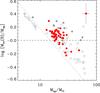 |
Fig. 16 Logarithmic ratio of evolutionary masses from bonnsai (Mev(B)) to spectroscopic masses (Msp), with the same symbols as in Fig. 14. Typical error bars are given in the upper right corner. The dashed line indicates points where Mev(B) = 15 M⊙. O2 stars were excluded. |
6.3. Wind properties
We also investigated the wind properties of our sample in the context of a wind-momentum – luminosity relationship (WLR, see Kudritzki et al. 1992, 1995), compared to past results and theoretical predictions.
The winds in the fastwind models used by the iacob-gbat are characterised by the wind-strength parameter, log Q (where Q = Ṁ(Rv∞)− 3/2). If estimates for the terminal velocities (v∞) and stellar radii (R) are available, then the log Q values from the spectral fits can be used to estimate mass-loss rates (Ṁ). However, we lack the UV spectroscopy required to estimate v∞ directly for our targets.
We therefore followed the same approach as Mokiem et al. (2007a,b), using our estimates of g and R to estimate the escape velocity (vesc): ![Mathematical equation: \begin{equation} v_{\rm esc}\,=\,\left[ 2gR(1-\Gamma) \right]^{1/2}, \end{equation}](/articles/aa/full_html/2017/05/aa29210-16/aa29210-16-eq57.png) (2)where Γ is the Eddington factor11. From this we obtained estimates of v∞, employing v∞/vesc = 2.65 (Kudritzki & Puls 2000), scaled to a metallicity of 0.5 Z⊙ by a factor of Z0.13 (Leitherer et al. 1992), leading to estimates of Ṁ via the Q-parameter. We then calculated the modified wind-momentum rates for our sample, Dmom = Ṁv∞R1/2, which are shown as a function of stellar luminosity in Fig. 17. Our results follow the expected linear trend from Vink et al. (2001), with log Dmom increasing with luminosity. We now discuss our results in two groups, separated at log L/L⊙ ~ 5.1, as indicated in Fig. 17.
(2)where Γ is the Eddington factor11. From this we obtained estimates of v∞, employing v∞/vesc = 2.65 (Kudritzki & Puls 2000), scaled to a metallicity of 0.5 Z⊙ by a factor of Z0.13 (Leitherer et al. 1992), leading to estimates of Ṁ via the Q-parameter. We then calculated the modified wind-momentum rates for our sample, Dmom = Ṁv∞R1/2, which are shown as a function of stellar luminosity in Fig. 17. Our results follow the expected linear trend from Vink et al. (2001), with log Dmom increasing with luminosity. We now discuss our results in two groups, separated at log L/L⊙ ~ 5.1, as indicated in Fig. 17.
6.3.1. log L/L⊙≥ 5.1
For the more luminous stars in our sample we were generally able to arrive at reliable estimates of log Q and therefore estimate Ṁ and Dmom. For a WLR of the form log Dmom = x log L/L⊙ + D0, we obtain x = 1.07 ± 0.18 and D0 = 22.67 ± 0.99 from a linear fit to our results for log L/L⊙ ≥ 5.1. These values differ from those from Mokiem et al. (2007b), who obtained x = 1.87 ± 0.19 and D0 = 18.30 ± 1.04, in good agreement with predictions from Vink et al. (2001).
These differences may have two origins. A first factor might be the inhomogeneity of the Mokiem et al. sample, which included more luminous stars as well as dwarfs. In the standard theory of radiatively driven winds, luminosity class should not play a role (Kudritzki & Puls 2000), but clumping may introduce a differential effect. Some of the luminous stars studied by Mokiem et al. had large wind momenta, possibly reflecting the impact of significant clumping. When corrected for clumping in selected objects (following Repolust et al. 2004), they found x = 1.49 ± 0.18 and D0 = 20.40 ± 1.00, in much better agreement with our values. This effect is reinforced by the strong dependence of Ṁ on Γ. Vink et al. (2011) and Gräfener et al. (2011) have argued that there is a kink in the relationship between Ṁ and Γe at log Γe ~ −0.58, when the effect of Γ sets in. The result is increased Ṁ for supergiants as compared to dwarfs, as for instance shown by the low Γe supergiants compared to their dwarf counterparts in Fig. 8 from Bestenlehner et al. (2014). Thus, the WLR slope obtained by Mokiem et al. will be steeper because of the influence of supergiants close to the Eddington limit.
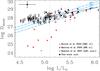 |
Fig. 17 Wind-momentum–luminosity relationship (WLR) for our sample compared with theoretical predictions from Vink et al. (2001) for the metallicities of the Milky Way and the Magellanic Clouds. Stars with upper limits on log Q (hence Dmom) are plotted with open symbols, and those analysed using the nitrogen lines are plotted with diamonds. Typical uncertainties are shown in the upper left corner, and the vertical dashed line indicates log L/L⊙ = 5.1. Results from Bouret et al. (2003), Martins et al. (2005), and Mokiem et al. (2007a) for their samples of O dwarfs in the SMC, MW, and LMC O, respectively, are plotted in red; the use of clumped (“cl.”) or unclumped (“uncl.”) wind models in each work is also indicated in the legend. |
Secondly, at slightly lower luminosities, when the Mokiem et al. sample was also dominated by dwarfs, they obtained estimates for β (the exponent of the wind velocity-law) that were larger than the 0.8 adopted in our study. Lower β means faster wind acceleration and higher velocities in the region where Hα and He ii λ 4686 are formed, leading to higher mass-loss rates (for a discussion of the dependence of the derived mass-loss rate on β, see Markova et al. 2004). An example of how this can reconcile the derived WLRs is given by Ramírez-Agudelo (2017).
In short, both effects push our estimated WLR to a smaller slope and a larger vertical offset than that from Mokiem et al. We thus find a flatter slope for the WLR (also flatter than theoretical expectations) that should be investigated further.
6.3.2. log L/L⊙ < 5.1
The winds of the less luminous stars in the LMC become thin, and the optical diagnostics (mainly Hα and He ii λ 4686) are insensitive to changes in density. We could therefore only derive upper limits on Dmom for stars with log L/L⊙ < 5.1 (except for one object fairly close to the log L/L⊙ = 5.1 boundary); similar problems were also encountered by Mokiem et al. (2007b).
We also include results in Fig. 17 for the SMC from Bouret et al. (2003) and Milky Way from Martins et al. (2005), who both found from UV diagnostics weaker winds than predicted by theory in this lower-luminosity regime. These stars remain a challenge for the theory of radiatively driven winds (see Puls et al. 2008). Several explanations for these weak winds have been proposed, such as X-rays (Herrero et al. 2009; Huenemoerder et al. 2012) or coronal winds (Lucy 2012), although the question remains open. A similar problem might be present even for some higher-luminosity stars, for example around log L/L⊙ ~ 5.5–5.6 in our results, although we note that both Bouret et al. and Martins et al. included clumped winds in their analyses, which led to lower mass-loss rates.
To obtain better constraints on the wind properties of the less luminous stars in our sample (and investigate if similarly weak winds are found as in other studies), we require UV spectroscopy spanning 1100–1800 Å, which contains diagnostic lines far more sensitive to wind effects than those available in the optical (particularly in the case of weak winds).
7. Summary and conclusions
In the framework of the VLT-FLAMES Tarantula Survey, we have analysed the optical spectra of 105 apparently single O-type dwarfs in the 30 Doradus region of the LMC. We used the iacob-gbat to estimate stellar and wind parameters for our sample, and used both classical techniques and the Bayesian bonnsai tool to estimate evolutionary masses. This study is the largest quantitative analysis of O dwarfs in the LMC, with the most complete coverage of spectral types to date. Our summary and conclusions are as follows:
-
We were only able to obtain upper limits on log Q for ~70% of the stars. Analysis using HHeN diagnostics was necessary in 20 cases because we lack reliable He i lines. In addition, we found indications of a possible binary nature in 14 stars through anomalously low helium abundances (Y(He) < 0.08), and 10 stars with relatively high gravities. The O2-type stars in our sample also show inconsistencies that could be related to multiplicity (and/or nitrogen peculiarities).
-
We provide a new effective temperature – spectral type calibration from a linear fit to our data (excluding O2 stars). We find good agreement with previous results, but are unable at present to reach a firm conclusion on the need for a separate, steeper relation for spectral types earlier than O4.
-
From H–R and Kiel diagrams of our sample (which mostly spans 3.8 < log g < 4.2) there appear to be relatively few stars younger than 1 Myr. Possible explanations include underestimated gravities from fastwind, missing stars still embedded in their natal clouds, or that the main episode of star formation in 30 Dor simply occurred 1 to 4 Myr ago.
-
Most of the rapid rotators (v sin i ≥ 250 km s-1) in our sample have masses below ~25 M⊙ and are closer to the ZAMS than the rest of the sample. Most are also located outside the NGC 2060 and NGC 2070 clusters, suggesting a potential runaway nature.
-
The fastest rotators (v sin i ≥ 340 km s-1) are found mostly at intermediate gravities (3.9 < log gc < 4.1), with none at lower gravities. We investigated if this was due to an observational bias, whereby lower-mass stars evolve out of the O-type sample as they age. We concluded that the estimated contribution of these additional stars is insufficient to explain the differences in the v sin i – log gc distribution at intermediate and lower gravities, and note that this behaviour is not predicted by current evolutionary models.
-
We compared evolutionary and spectroscopic mass estimates for the sample, finding a non-negligible number of stars with differences of 25 to 50%. We also found that the Mev/Msp ratio decreases with increasing Msp, typically with Mev > Msp for stars with Msp ≤ 20 M⊙, and Mev < Msp for Msp ≥ 30 M⊙. However, this trend is probably caused by a simple observational bias, whereby the O-type dwarfs all have Mev > 15 M⊙; similar results for early B-dwarfs from the VFTS will need to be included for a complete view of the estimated masses. We find no compelling evidence of a systematic mass discrepancy.
-
When we investigated the possible mass discrepancy, we noted that our gravities tended to be lower than those predicted by evolutionary models, which could be explained by the fact that bonnsai takes into account that stars spend more time near the ZAMS than far away from it, which might favour slightly higher gravities.
-
At log L/L⊙ > 5.1 our stars have a high dispersion in the WLR, although the majority are consistent with theoretical predictions for the LMC within the estimated uncertainties. Unclumped models and the large uncertainty on the adopted terminal velocities could explain stars with winds apparently stronger than the theoretical WLR for Galactic metallicity, but there is no satisfactory explanation for those stars with winds estimated to be weaker than predicted for the SMC. We obtain a flatter fit to the WLR compared to that from Mokiem et al. (2007b), probably because their study also included O-type supergiants close to the Eddington limit. At log L/L⊙ < 5.1 we could not reliably estimate log Q for our sample because of the current lack of UV observations.
O Vz stars are characterised by He ii λ 4686 absorption stronger than any other helium line in their optical spectra (Walborn 2009).
From the “Proper motions of massive stars in 30 Doradus” program (GO 12499, P. I.: D. J. Lennon).
The grid was computed using the Condor workload management system (http://www.cs.wisc.edu/condor/) implemented at the Instituto de Astrofísica de Canarias.
log gc is defined as the logarithmic gravity derived from the spectral analysis corrected for centrifugal effects (see e.g. Herrero et al. 1992; Repolust et al. 2004).
Y(He) is the helium-to-hydrogen number fraction, Y(He) = N(He)/N(H).
The bonnsai web-service is available at http://www.astro.uni-bonn.de/stars/bonnsai
Five stars for which photometry was unavailable are not included.
VFTS 072, 169, 216, 468, 506, 621, 755, and 797.
For a complete description see Schneider et al. (2014).
Defined here as the ratio of radiative acceleration due to Thomson scattering compared to gravity, Γ = 5.765×10⁻¹⁶
 , where Y is the helium-to- hydrogen number fraction.
Acknowledgments
C.S.-S. acknowledges support from the Joint Committee ESO-Government of Chile and DIDULS programme from Universidad de La Serena under grant DIDULS Regular PR16145. S.S.-D. and A.H. acknowledge support from the Spanish Ministry of Economy and Competitiveness (MINECO) under grants AYA2015-68012-C2-1 and SEV-2015-0548. This paper made use of the IAC Supercomputing facility HTCondor (http://research.cs.wisc.edu/htcondor/), recently expanded and improved thanks to FEDER funds granted by the Ministry of Economy and Competitiveness, project code IACA13-3E-2493. O.H.R.-A. acknowledges funding from the European Union’s Horizon 2020 research and innovation programme under the Marie Skłodowska-Curie grant agreement No. 665593 awarded to the Science and Technology Facilities Council. N.J.G. is part of the International Max Planck Research School (IMPRS) for Astronomy and Astrophysics at the Universities of Bonn and Cologne. STScI is operated by the Association of Universities for Research in Astronomy, Inc., under NASA contract NAS5-26555.
References
- Aldoretta, E. J., Caballero-Nieves, S. M., Gies, D. R., et al. 2015, AJ, 149, 26 [NASA ADS] [CrossRef] [Google Scholar]
- Bestenlehner, J. M., Vink, J. S., Gräfener, G., et al. 2011, A&A, 530, L14 [NASA ADS] [CrossRef] [EDP Sciences] [Google Scholar]
- Bestenlehner, J. M., Gräfener, G., Vink, J. S., et al. 2014, A&A, 570, A38 [NASA ADS] [CrossRef] [EDP Sciences] [Google Scholar]
- Bouret, J.-C., Lanz, T., Hillier, D. J., et al. 2003, ApJ, 595, 1182 [NASA ADS] [CrossRef] [Google Scholar]
- Bromm, V., Yoshida, N., Hernquist, L., & McKee, C. F. 2009, Nature, 459, 49 [NASA ADS] [CrossRef] [PubMed] [Google Scholar]
- Brott, I., de Mink, S. E., Cantiello, M., et al. 2011, A&A, 530, A115 [NASA ADS] [CrossRef] [EDP Sciences] [Google Scholar]
- Castro, N., Urbaneja, M. A., Herrero, A., et al. 2012, A&A, 542, A79 [NASA ADS] [CrossRef] [EDP Sciences] [Google Scholar]
- Castro, N., Fossati, L., Langer, N., et al. 2014, A&A, 570, L13 [NASA ADS] [CrossRef] [EDP Sciences] [Google Scholar]
- Crowther, P. A., Caballero-Nieves, S. M., Bostroem, K. A., et al. 2016, MNRAS, 458, 624 [NASA ADS] [CrossRef] [Google Scholar]
- de Mink, S. E., Langer, N., Izzard, R. G., Sana, H., & de Koter, A. 2013, ApJ, 764, 166 [NASA ADS] [CrossRef] [Google Scholar]
- de Mink, S. E., Sana, H., Langer, N., Izzard, R. G., & Schneider, F. R. N. 2014, ApJ, 782, 7 [NASA ADS] [CrossRef] [Google Scholar]
- Denissenkov, P. A. 1994, A&A, 287, 113 [NASA ADS] [Google Scholar]
- Doran, E. I., & Crowther, P. A. 2011, Bull. Soc. Roy. Sci. Liège, 80, 129 [NASA ADS] [Google Scholar]
- Doran, E. I., Crowther, P. A., de Koter, A., et al. 2013, A&A, 558, A134 [NASA ADS] [CrossRef] [EDP Sciences] [Google Scholar]
- Dufton, P. L., Dunstall, P. R., Evans, C. J., et al. 2011, ApJ, 743, L22 [NASA ADS] [CrossRef] [Google Scholar]
- Dufton, P. L., Langer, N., Dunstall, P. R., et al. 2013, A&A, 550, A109 [NASA ADS] [CrossRef] [EDP Sciences] [Google Scholar]
- Dunstall, P. R., Dufton, P. L., Sana, H., et al. 2015, A&A, 580, A93 [NASA ADS] [CrossRef] [EDP Sciences] [Google Scholar]
- Ekström, S., Georgy, C., Eggenberger, P., et al. 2012, A&A, 537, A146 [NASA ADS] [CrossRef] [EDP Sciences] [Google Scholar]
- Evans, C. J., Taylor, W. D., Hénault-Brunet, V., et al. 2011, A&A, 530, A108 [NASA ADS] [CrossRef] [EDP Sciences] [Google Scholar]
- Evans, C. J., Hainich, R., Oskinova, L. M., et al. 2012, ApJ, 753, 173 [NASA ADS] [CrossRef] [Google Scholar]
- Evans, C. J., Kennedy, M. B., Dufton, P. L., et al. 2015, A&A, 574, A13 [NASA ADS] [CrossRef] [EDP Sciences] [Google Scholar]
- Fullerton, A. W., Massa, D. L., & Prinja, R. K. 2006, ApJ, 637, 1025 [NASA ADS] [CrossRef] [Google Scholar]
- Gibson, B. K. 2000, Mem. Soc. Astron. Italiana, 71, 693 [Google Scholar]
- Gräfener, G., Vink, J. S., de Koter, A., & Langer, N. 2011, A&A, 535, A56 [NASA ADS] [CrossRef] [EDP Sciences] [Google Scholar]
- Gray, D. F. 2005, The Observation and Analysis of Stellar Photospheres, 3rd edn. (UK: Cambridge University Press) [Google Scholar]
- Grin, N. J., Ramirez-Agudelo, O. H., de Koter, A., et al. 2017, A&A, 600, A82 [NASA ADS] [CrossRef] [EDP Sciences] [Google Scholar]
- Groenewegen, M. A. T., Lamers, H. J. G. L. M., & Pauldrach, A. W. A. 1989, A&A, 221, 78 [NASA ADS] [Google Scholar]
- Hanson, M. M. 1998, in Properties of Hot Luminous Stars, ed. I. Howarth, ASP Conf. Ser., 131, 1 [Google Scholar]
- Herrero, A., Kudritzki, R. P., Vilchez, J. M., et al. 1992, A&A, 261, 209 [NASA ADS] [Google Scholar]
- Herrero, A., Corral, L. J., Villamariz, M. R., & Martín, E. L. 1999, A&A, 348, 542 [NASA ADS] [Google Scholar]
- Herrero, A., Puls, J., & Najarro, F. 2002, A&A, 396, 949 [NASA ADS] [CrossRef] [EDP Sciences] [Google Scholar]
- Herrero, A., Garcia, M., & Najarro, F. 2009, Ap&SS, 320, 149 [NASA ADS] [CrossRef] [Google Scholar]
- Hillier, D. J. 1991, A&A, 247, 455 [NASA ADS] [Google Scholar]
- Hillier, D. J., & Miller, D. L. 1998, ApJ, 496, 407 [NASA ADS] [CrossRef] [Google Scholar]
- Huenemoerder, D. P., Oskinova, L. M., Ignace, R., et al. 2012, ApJ, 756, L34 [NASA ADS] [CrossRef] [Google Scholar]
- Hunter, I., Brott, I., Lennon, D. J., et al. 2008, ApJ, 676, L29 [NASA ADS] [CrossRef] [Google Scholar]
- Ilee, J. D., Cyganowski, C. J., Nazari, P., et al. 2016, MNRAS, 462, 4386 [NASA ADS] [CrossRef] [Google Scholar]
- Köhler, K., Langer, N., de Koter, A., et al. 2015, A&A, 573, A71 [NASA ADS] [CrossRef] [EDP Sciences] [Google Scholar]
- Kudritzki, R.-P. 1980, A&A, 85, 174 [NASA ADS] [Google Scholar]
- Kudritzki, R.-P., & Puls, J. 2000, ARA&A, 38, 613 [NASA ADS] [CrossRef] [Google Scholar]
- Kudritzki, R.-P., Hummer, D. G., Pauldrach, A. W. A., et al. 1992, A&A, 257, 655 [NASA ADS] [Google Scholar]
- Kudritzki, R.-P., Lennon, D. J., & Puls, J. 1995, in Science with the VLT, eds. J. R. Walsh, & I. J. Danziger (Heidelberg: Springer), 246 [Google Scholar]
- Kudritzki, R.-P., Urbaneja, M. A., Bresolin, F., et al. 2008, ApJ, 681, 269 [NASA ADS] [CrossRef] [Google Scholar]
- Kudritzki, R.-P., Urbaneja, M. A., Gazak, Z., et al. 2013, ApJ, 779, L20 [NASA ADS] [CrossRef] [Google Scholar]
- Kuiper, N. H. 1960, Proceedings of the Koninklijke Nederlandse Akademie van Wetenschappen, 63, 38 [Google Scholar]
- Langer, N. 1992, A&A, 265, L17 [NASA ADS] [Google Scholar]
- Langer, N. 2012, ARA&A, 50, 107 [NASA ADS] [CrossRef] [Google Scholar]
- Langer, N., & Kudritzki, R. P. 2014, A&A, 564, A52 [NASA ADS] [CrossRef] [EDP Sciences] [Google Scholar]
- Langer, N., Cantiello, M., Yoon, S.-C., et al. 2008, in IAU Symp. 250, eds. F. Bresolin, P. A. Crowther, & J. Puls, 167 [Google Scholar]
- Lefever, K., Puls, J., & Aerts, C. 2007, in The Future of Photometric, Spectrophotometric and Polarimetric Standardization, ed. C. Sterken, ASP Conf. Ser., 364, 545 [Google Scholar]
- Leitherer, C., Robert, C., & Drissen, L. 1992, ApJ, 401, 596 [NASA ADS] [CrossRef] [Google Scholar]
- Lucy, L. B. 2012, A&A, 544, A120 [NASA ADS] [CrossRef] [EDP Sciences] [Google Scholar]
- Maeder, A. 1987, A&A, 173, 247 [NASA ADS] [Google Scholar]
- Maeder, A., & Meynet, G. 2000, ARA&A, 38, 143 [NASA ADS] [CrossRef] [Google Scholar]
- Mahy, L., Rauw, G., De Becker, M., Eenens, P., & Flores, C. A. 2015, A&A, 577, A23 [NASA ADS] [CrossRef] [EDP Sciences] [Google Scholar]
- Maíz Apellániz, J. 2004, PASP, 116, 859 [NASA ADS] [CrossRef] [Google Scholar]
- Maíz Apellániz, J., Evans, C. J., Barbá, R. H., et al. 2014, A&A, 564, A63 [NASA ADS] [CrossRef] [EDP Sciences] [Google Scholar]
- Markova, N., Puls, J., Repolust, T., & Markov, H. 2004, A&A, 413, 693 [NASA ADS] [CrossRef] [EDP Sciences] [Google Scholar]
- Martins, F., Schaerer, D., Hillier, D. J., et al. 2005, A&A, 441, 735 [NASA ADS] [CrossRef] [EDP Sciences] [Google Scholar]
- Mason, B. D., Gies, D. R., Hartkopf, W. I., et al. 1998, AJ, 115, 821 [NASA ADS] [CrossRef] [Google Scholar]
- Mason, B. D., Hartkopf, W. I., Gies, D. R., Henry, T. J., & Helsel, J. W. 2009, AJ, 137, 3358 [NASA ADS] [CrossRef] [EDP Sciences] [Google Scholar]
- Massey, P., Bresolin, F., Kudritzki, R. P., Puls, J., & Pauldrach, A. W. A. 2004, ApJ, 608, 1001 [Google Scholar]
- Massey, P., Puls, J., Pauldrach, A. W. A., et al. 2005, ApJ, 627, 477 [NASA ADS] [CrossRef] [Google Scholar]
- Massey, P., Zangari, A. M., Morrell, N. I., et al. 2009, ApJ, 692, 618 [NASA ADS] [CrossRef] [Google Scholar]
- Massey, P., Neugent, K. F., Hillier, D. J., & Puls, J. 2013, ApJ, 768, 6 [NASA ADS] [CrossRef] [Google Scholar]
- Mokiem, M. R., de Koter, A., Evans, C. J., et al. 2007a, A&A, 465, 1003 [NASA ADS] [CrossRef] [EDP Sciences] [Google Scholar]
- Mokiem, M. R., de Koter, A., Vink, J. S., et al. 2007b, A&A, 473, 603 [NASA ADS] [CrossRef] [EDP Sciences] [Google Scholar]
- Morel, T., Castro, N., Fossati, L., et al. 2015, in New Windows on Massive Stars, eds. G. Meynet, C. Georgy, J. Groh, & P. Stee, IAU Symp., 307, 342 [Google Scholar]
- Morrell, N. I., Massey, P., Neugent, K. F., Penny, L. R., & Gies, D. R. 2014, ApJ, 789, 139 [NASA ADS] [CrossRef] [Google Scholar]
- Muijres, L. E., Vink, J. S., de Koter, A., Müller, P. E., & Langer, N. 2012, A&A, 537, A37 [NASA ADS] [CrossRef] [EDP Sciences] [Google Scholar]
- Müller, P. E., & Vink, J. S. 2014, A&A, 564, A57 [NASA ADS] [CrossRef] [EDP Sciences] [Google Scholar]
- Packet, W. 1981, A&A, 102, 17 [NASA ADS] [Google Scholar]
- Pasquini, L., Avila, G., Blecha, A., et al. 2002, The Messenger, 110, 1 [NASA ADS] [Google Scholar]
- Petit, V., Keszthelyi, Z., MacInnis, R., et al. 2017, MNRAS, 466, 1052 [NASA ADS] [CrossRef] [Google Scholar]
- Platais, I., van der Marel, R. P., Lennon, D. J., et al. 2015, AJ, 150, 89 [NASA ADS] [CrossRef] [Google Scholar]
- Puls, J., Urbaneja, M. A., Venero, R., et al. 2005, A&A, 435, 669 [NASA ADS] [CrossRef] [EDP Sciences] [Google Scholar]
- Puls, J., Markova, N., Scuderi, S., et al. 2006, A&A, 454, 625 [NASA ADS] [CrossRef] [EDP Sciences] [Google Scholar]
- Puls, J., Vink, J. S., & Najarro, F. 2008, A&ARv, 16, 209 [NASA ADS] [CrossRef] [EDP Sciences] [Google Scholar]
- Ramírez-Agudelo, O. H., Simón-Díaz, S., Sana, H., et al. 2013, A&A, 560, A29 [NASA ADS] [CrossRef] [EDP Sciences] [Google Scholar]
- Ramírez-Agudelo, O. H., Sana, H., de Mink, S. E., et al. 2015, A&A, 580, A92 [NASA ADS] [CrossRef] [EDP Sciences] [Google Scholar]
- Ramírez-Agudelo, O. H., Sana, H., de Koter, A., et al. 2017, A&A, 600, A81 [NASA ADS] [CrossRef] [EDP Sciences] [Google Scholar]
- Repolust, T., Puls, J., & Herrero, A. 2004, A&A, 415, 349 [NASA ADS] [CrossRef] [EDP Sciences] [Google Scholar]
- Rivero González, J. G., Puls, J., & Najarro, F. 2011, A&A, 536, A58 [NASA ADS] [CrossRef] [EDP Sciences] [Google Scholar]
- Rivero González, J. G., Puls, J., Massey, P., & Najarro, F. 2012a, A&A, 543, A95 [NASA ADS] [CrossRef] [EDP Sciences] [Google Scholar]
- Rivero González, J. G., Puls, J., Najarro, F., & Brott, I. 2012b, A&A, 537, A79 [NASA ADS] [CrossRef] [EDP Sciences] [Google Scholar]
- Sabbi, E., Lennon, D. J., Gieles, M., et al. 2012, ApJ, 754, L37 [NASA ADS] [CrossRef] [Google Scholar]
- Sabín-Sanjulián, C., Simón-Díaz, S., Herrero, A., et al. 2014, A&A, 564, A39 [NASA ADS] [CrossRef] [EDP Sciences] [Google Scholar]
- Sabbi, E., Lennon, D. J., Anderson, J., et al. 2016, ApJS, 222, 11 [NASA ADS] [CrossRef] [Google Scholar]
- Salpeter, E. E. 1955, ApJ, 121, 161 [Google Scholar]
- Sana, H., de Mink, S. E., de Koter, A., et al. 2012, Science, 337, 444 [Google Scholar]
- Sana, H., de Koter, A., de Mink, S. E., et al. 2013, A&A, 550, A107 [NASA ADS] [CrossRef] [EDP Sciences] [Google Scholar]
- Sana, H., Le Bouquin, J.-B., Lacour, S., et al. 2014, ApJS, 215, 15 [NASA ADS] [CrossRef] [Google Scholar]
- Santolaya-Rey, A. E., Puls, J., & Herrero, A. 1997, A&A, 323, 488 [NASA ADS] [Google Scholar]
- Schneider, F. R. N., Langer, N., de Koter, A., et al. 2014, A&A, 570, A66 [Google Scholar]
- Schneider, F. R. N., Podsiadlowski, P., Langer, N., Castro, N., & Fossati, L. 2016, MNRAS, 457, 2355 [NASA ADS] [CrossRef] [Google Scholar]
- Simón-Díaz, S., & Herrero, A. 2014, A&A, 562, A135 [NASA ADS] [CrossRef] [EDP Sciences] [Google Scholar]
- Simón-Díaz, S., Castro, N., Herrero, A., et al. 2011, J. Phys. Conf. Ser., 328, 012021 [NASA ADS] [CrossRef] [Google Scholar]
- Simón-Díaz, S., Herrero, A., Sabín-Sanjulián, C., et al. 2014, A&A, 570, L6 [NASA ADS] [CrossRef] [EDP Sciences] [Google Scholar]
- Simón-Díaz, S., Godart, M., Castro, N., et al. 2017, A&A, 597, A22 [NASA ADS] [CrossRef] [EDP Sciences] [Google Scholar]
- Sota, A., Maíz Apellániz, J., Walborn, N. R., et al. 2011, ApJS, 193, 24 [NASA ADS] [CrossRef] [Google Scholar]
- Sota, A., Maíz Apellániz, J., Morrell, N. I., et al. 2014, ApJS, 211, 10 [NASA ADS] [CrossRef] [Google Scholar]
- Sundqvist, J. O., Puls, J., & Owocki, S. P. 2014, A&A, 568, A59 [NASA ADS] [CrossRef] [EDP Sciences] [Google Scholar]
- Šurlan, B., Hamann, W.-R., Aret, A., et al. 2013, A&A, 559, A130 [NASA ADS] [CrossRef] [EDP Sciences] [Google Scholar]
- Vink, J. S. 2012, in Death of Massive Stars: Supernovae and Gamma-Ray Bursts, eds. P. Roming, N. Kawai, & E. Pian, IAU Symp., 279, 29 [Google Scholar]
- Vink, J. S., de Koter, A., & Lamers, H. J. G. L. M. 2001, A&A, 369, 574 [NASA ADS] [CrossRef] [EDP Sciences] [Google Scholar]
- Vink, J. S., Muijres, L. E., Anthonisse, B., et al. 2011, A&A, 531, A132 [NASA ADS] [CrossRef] [EDP Sciences] [Google Scholar]
- Wade, G. A., & MiMeS Collaboration. 2015, in Physics and Evolution of Magnetic and Related Stars, eds. Y. Y. Balega, I. I. Romanyuk, & D. O. Kudryavtsev, ASP Conf. Ser., 494, 30 [Google Scholar]
- Wade, G. A., Neiner, C., Alecian, E., et al. 2016, MNRAS, 456, 2 [NASA ADS] [CrossRef] [Google Scholar]
- Walborn, N. R. 2009, in Massive Stars: From Pop III and GRBs to the Milky Way, Space Telescope Science Institute Symposium Series No. 20, eds. M. Livio, & E. Villaver (Cambridge University Press), 167 [Google Scholar]
- Walborn, N. R., Drissen, L., Parker, J. W., et al. 1999, AJ, 118, 1684 [NASA ADS] [CrossRef] [Google Scholar]
- Walborn, N. R., Howarth, I. D., Lennon, D. J., et al. 2002a, AJ, 123, 2754 [NASA ADS] [CrossRef] [Google Scholar]
- Walborn, N. R., Maíz-Apellániz, J., & Barbá, R. H. 2002b, AJ, 124, 1601 [NASA ADS] [CrossRef] [Google Scholar]
- Walborn, N. R., Sana, H., Taylor, W. D., Simón-Díaz, S., & Evans, C. J. 2012, in Proceedings of a Scientific Meeting in Honor of Anthony F. J. Moffat, eds. L. Drissen, C. Rubert, N. St-Louis, & A. F. J. Moffat, ASP Conf. Ser., 465, 490 [Google Scholar]
- Walborn, N. R., Sana, H., Simón-Díaz, S., et al. 2014, A&A, 564, A40 [NASA ADS] [CrossRef] [EDP Sciences] [Google Scholar]
- Weidner, C., & Vink, J. S. 2010, A&A, 524, A98 [NASA ADS] [CrossRef] [EDP Sciences] [Google Scholar]
- Woosley, S. E., & Heger, A. 2006, ApJ, 637, 914 [NASA ADS] [CrossRef] [Google Scholar]
- Woosley, S. E., Heger, A., & Weaver, T. A. 2002, Rev. Mod. Phys., 74, 1015 [NASA ADS] [CrossRef] [Google Scholar]
- Yorke, H. W. 1986, ARA&A, 24, 49 [NASA ADS] [CrossRef] [Google Scholar]
- Zinnecker, H., & Yorke, H. W. 2007, ARA&A, 45, 481 [NASA ADS] [CrossRef] [Google Scholar]
Appendix A: Stellar and wind parameters
Stellar and wind parameters obtained from quantitative analysis of our sample of O dwarfs.
First estimates of stellar and wind parameters from HHeN analysis of stars for which He i/ii analysis alone was considered unreliable.
Appendix B: Stellar radii, luminosities, and masses
Radii, luminosities, and spectroscopic masses obtained from our analysis, and evolutionary masses estimated from the Kiel (GT) and H–R (LT) diagrams and from the bonnsai tool (B).
First estimates of radii, luminosities, and spectroscopic masses obtained from HHeN analysis, and evolutionary masses estimated from the Kiel (GT) and H–R (LT) diagrams and from the bonnsai tool (B), for the subsample of stars for which He i/ii analysis alone was considered unreliable.
All Tables
Spectral coverage and resolving power (R) of each setting in the FLAMES–Medusa mode used by the VFTS.
Number of stars in our analysis with problematic χ2 distributions of wind strength (log Q), effective temperature (Teff), helium abundance (Y(He)), and surface gravity (log g) caused by degeneracies or because they reach the boundaries of the grid.
Stellar and wind parameters obtained from quantitative analysis of our sample of O dwarfs.
First estimates of stellar and wind parameters from HHeN analysis of stars for which He i/ii analysis alone was considered unreliable.
Radii, luminosities, and spectroscopic masses obtained from our analysis, and evolutionary masses estimated from the Kiel (GT) and H–R (LT) diagrams and from the bonnsai tool (B).
First estimates of radii, luminosities, and spectroscopic masses obtained from HHeN analysis, and evolutionary masses estimated from the Kiel (GT) and H–R (LT) diagrams and from the bonnsai tool (B), for the subsample of stars for which He i/ii analysis alone was considered unreliable.
All Figures
|
Fig. 1 Spectral type distributions for the O-type stars. The whole sample is shown in the upper left panel in black. The remaining panels show the spectral type distribution for the luminosity subclasses within the sample: O V stars in blue, O IV, O III–IV, and O V–III in green, O Vz in red (and O Vz? by the grey hatched areas). |
| In the text | |
|
Fig. 2 Spatial distribution of our sample stars in 30 Dor. Luminosity subclasses are indicated as follows: blue circles for O V stars, red triangles for O Vz stars (including those with doubtful V/Vz classifications), and green squares for O IV stars (including V–III and III–IV classes). The central and southwestern orange circles (with adopted radii of 2.́4, see e.g. Sana et al. 2013) indicate the approximate extent of NGC 2070 and NGC 2060, respectively. |
| In the text | |
|
Fig. 3 Example O-type dwarf spectra for the range of luminosity subclasses in our sample (IV, III–IV, V–III, V, and Vz); the diagnostic H and He lines are indicated. The uppermost spectrum (VFTS 096) suffers from stellar contamination in the Medusa fibre (see Fig. 4 and Sect. 4.3.1). |
| In the text | |
|
Fig. 4 Example HST/WFC3 images of O dwarf stars in the VFTS. The aperture of the Medusa fibres (1.̋2) is indicated by the inner green circles; the outer circles have twice this diameter to help guide the eye. VFTS 021 is shown as an example of a uncontaminated Medusa fibre, while the spectra of the others shown here are expected to have some degree of contamination from close-by companions. |
| In the text | |
|
Fig. 5 Model fits to the spectrum of VFTS 621, with the best fit from the HHe (Teff = 36 kK, log g = 3.8) and HHeN (Teff = 54 kK, log g = 4.2) analyses shown in red and blue, respectively. The log Q as well as the helium and nitrogen abundances are the same in both models. These single-star models both suffer deficiencies that are suggestive of a composite observed spectrum, as seen in HST images (Fig. 4). |
| In the text | |
|
Fig. 6 Kiel (left) and H–R (right) diagrams for our sample. Class V objects are plotted in black, those with other luminosity classes (IV, III–IV, and V–III) in red. Stars analysed using HHeN lines are plotted as diamonds, while those with (stellar) contamination in the fibre aperture (see Sect. 4.3.1) are plotted as open symbols. Evolutionary tracks and isochrones for the LMC are from Brott et al. (2011) and Köhler et al. (2015), with an initial rotational velocity of 171 km s-1 (see Sect. 6.1). The zero-age main-sequence (ZAMS) is indicated in the two plots by the bold black line, and typical uncertainties are indicated in the upper and lower corner, respectively. |
| In the text | |
|
Fig. 7 Estimated effective temperatures (Teff) and rotation-corrected gravities (log gc) for our sample as a function of spectral subtype (using the same symbols as in Fig. 6); small shifts have been added to the abscissae of each star to avoid overlap. The upper panel shows the number of stars per subtype. |
| In the text | |
|
Fig. 8 Effective-temperature scale for our sample of stars (in grey) compared with results from Rivero González et al. (2011, 2012b,a), Mokiem et al. (2007a), and Massey et al. (2005). |
| In the text | |
|
Fig. 9 Comparison of our Teff calibration for O dwarfs in the LMC with those derived by Rivero González et al. (2012a,b) and adopted by Doran et al. (2013). Grey dots and bars represent the mean value and standard deviation of our Teff estimates for each spectral type, with our linear fit shown by the black line (and the grey zones indicating the associated uncertainties). |
| In the text | |
|
Fig. 10 Projected rotational velocities for our sample of O-type dwarfs. Fourteen stars have v sin i > 250 km s-1 (with the velocity threshold indicated by the vertical dashed line). |
| In the text | |
|
Fig. 11 Left: projected rotational velocities (v sin i) vs. rotation-corrected gravities (log gc) for our sample, grouped according to helium abundance. Theoretical predictions for the LMC from Brott et al. (2011) are shown in grey (for three initial masses and two initial rotational velocities as indicated). Predictions for solar metallicity and an initial vini of 40% the critical velocity from Ekström et al. (2012) are shown in blue. Right: v sin i distributions for three ranges of gravity: (1) low (log gc < 3.9); (2) intermediate (3.9 ≤ log gc ≤ 4.1); and (3) high (log gc > 4.1). |
| In the text | |
|
Fig. 12 Kiel (left) and H–R (right) diagrams for our sample grouped according to v sin i. Black filled circles: v sin i < 250 km s-1; red open circles: v sin i ≥ 250 km s-1. Evolutionary tracks and isochrones for an initial v sin i = 171 km s-1 from Brott et al. (2011) are also shown. |
| In the text | |
|
Fig. 13 Evolutionary masses (Mev) estimated using the H–R (Mev(LT), red crosses) and Kiel diagrams (Mev(GT), black dots) compared to those from bonnsai (Mev(B)). Error bars are shown in the upper left corner. The dashed line traces the one-to-one ratio, with differences of ±10% and 20% shown by the dotted lines. O2 stars are not included here. |
| In the text | |
|
Fig. 14 Evolutionary-mass estimates from bonnsai (Mev(B)) vs. spectroscopic masses (Msp). Grey open symbols: possible single-lined spectroscopic binaries (Sana et al. 2013; Walborn et al. 2014), stars with poor fits to He lines, high gravities (log g > 4.2) or low helium abundance, and objects with possible or confirmed fibre contamination. Filled grey symbols: objects from HHeN analysis and no indications of binarity or fibre contamination. Red symbols: rest of the sample. The dashed grey line indicates the one-to-one relation, with ±25 and ±50% shown by the dotted lines. Typical error bars are given in the upper left corner. O2 stars were excluded. |
| In the text | |
|
Fig. 15 Differences between gravities derived from bonnsai and those obtained from the spectroscopic analysis (log gc) as a function of the latter (left-hand panel) and spectroscopic mass (Msp, right-hand panel). The dashed lines mark the ±2σ region used to calculate the mean differences; symbols have the same meaning as in Fig. 14. O2 stars were excluded. |
| In the text | |
|
Fig. 16 Logarithmic ratio of evolutionary masses from bonnsai (Mev(B)) to spectroscopic masses (Msp), with the same symbols as in Fig. 14. Typical error bars are given in the upper right corner. The dashed line indicates points where Mev(B) = 15 M⊙. O2 stars were excluded. |
| In the text | |
|
Fig. 17 Wind-momentum–luminosity relationship (WLR) for our sample compared with theoretical predictions from Vink et al. (2001) for the metallicities of the Milky Way and the Magellanic Clouds. Stars with upper limits on log Q (hence Dmom) are plotted with open symbols, and those analysed using the nitrogen lines are plotted with diamonds. Typical uncertainties are shown in the upper left corner, and the vertical dashed line indicates log L/L⊙ = 5.1. Results from Bouret et al. (2003), Martins et al. (2005), and Mokiem et al. (2007a) for their samples of O dwarfs in the SMC, MW, and LMC O, respectively, are plotted in red; the use of clumped (“cl.”) or unclumped (“uncl.”) wind models in each work is also indicated in the legend. |
| In the text | |
Current usage metrics show cumulative count of Article Views (full-text article views including HTML views, PDF and ePub downloads, according to the available data) and Abstracts Views on Vision4Press platform.
Data correspond to usage on the plateform after 2015. The current usage metrics is available 48-96 hours after online publication and is updated daily on week days.
Initial download of the metrics may take a while.