© ESO, 2016

1. Introduction

The understanding of stellar activity and its impact on convection is an important challenge when studying the impact of stellar activity on exoplanet detectability because the variability of the convection attenuation impacts stellar radial velocities (RVs). In the solar case, the inhibition of convection by magnetic fields indeed dominates the stellar signal (Meunier et al. 2010a). This model has been confirmed with several observations: the reconstruction of the solar RV using Michelson Doppler Imager (MDI) Dopplergrams (Meunier et al. 2010b); more recently, RV variations of similar amplitude have been obtained using direct observations of the Sun (Dumusque et al. 2015) as well as using indirect solar RV measurements from various bodies in solar system observations (Moon, asteroids, Jupiter satellites) by Lanza et al. (2016) and Haywood et al. (2016).

In simulations made by Meunier et al. (2010a) based on observed solar features and later by Borgniet et al. (2015) based on simulated solar features, it was assumed that the solar convective blueshift was attenuated by a factor of two thirds, on average, in magnetic regions such as plages and the solar network, based on solar observations by Brandt & Solanki (1990). How stellar granulation changes with magnetic field for different stellar types is yet unknown. This is, however, a critical factor in estimating the impact of stellar type on the activity-induced RV variations, as already pointed out by Dravins & Nordlund (1990), for example by extrapolating the work of Borgniet et al. (2015) to stars other than the Sun.

The determination of the amplitude of the absolute convective blueshift depends on two parameters, for a given coverage by magnetic features: 1/ How does the convective blueshift depend on spectral type? 2/ Is the attenuation factor, due to magnetic fields, similar for all stars?

Concerning the first issue, a number of results in the literature already give some clues. Dravins et al. (1981) have shown that the dependancy of the velocity derived from each spectral line as a function of their depth is directly related to the properties of solar convection. Lines of different depths (intensities) form at different depths in the atmosphere: they are therefore probing regions with different intensity-velocity correlations inside granules, so that their sensitivity differs for different convective blueshifts. Two types of measurements reflect this process: 1/ the absolute shifts of spectral line bisectors; 2/ the differential velocity shifts of spectral lines (namely between lines of different depths). The first ones are difficult to measure because of other effects not easy to quantify at the required precision (except for the Sun). The latter seems to have a universal shape according to Gray (2009). Hamilton & Lester (1999) also show that the bottom of the line position is less sensitive to resolution effects compared to the bisector analysis, which is also interesting when studying a large sample of stars with different vsini, making it a powerful method to estimate these convection properties, something not possible by RV jitter analysis.

This property has been studied for stars other than the Sun (e.g. Gray 1982; Dravins 1987, 1999; Hamilton & Lester 1999; Landstreet 2007; Allende Prieto et al. 2002; Gray 2009) but always for a very small number of main sequence stars. The analysis has usually been performed using a very small number of lines, Gray (2009), or low signal to noise ratio (S/N) spectra. How the measurements are impacted by the choices of selected lines has not been investigated so far. These studies however show that velocity flows inside granules and resulting convective blueshifts increase with T_eff. Pasquini et al. (2011) have studied a larger sample but found a very large dispersion of the convective blueshift of the main sequence stars. On the other hand, recent hydrodynamical numerical simulations have been performed by Allende Prieto et al. (2013) and show a clear dependence of the convective blueshift on spectral type. Other groups have performed hydrodynamical simulations of granulation over a grid of stellar parameters; Magic et al. (2013, 2014), Trampedach et al. (2013), Tremblay et al. (2013), Beeck et al. (2013), but do not provide potentially useful values of the convective blueshift. Magic & Asplund (2014) however found larger granules (usually associated with larger velocity fields) for hotter stars, consistent with a larger convective blueshift. In principle both effects (absolute and differential velocity shifts) can be extracted from numerical simulations providing they model enough spectral lines: this is discussed in Sect. 4.

Concerning the second issue however, it is mostly uncharted and no previous study has estimated whether the response of the granulation to magnetic field depends on the spectral type or not. Several studies have aimed at measuring the temperature variations of individual stars during stellar cycles (Gray et al. 1992; Gray & Baliunas 1994, 1995; Gray et al. 1996b,a), yet no systematic tendency is available today.

In this paper we therefore focus on this last aspect. We aimed to precisely estimate the convective blueshift for a large sample of G-K main sequence stars but also measure how this blueshift varies with magnetic activity. To this end, we measured the differential velocity shifts of spectral lines, and more specifically their slope, defined in a robust way, in order to estimate the amplitude of granulation for each star. After a description of our data analysis in Sect. 2, we derive the dependency on spectral type and activity level of the granulation amplitude using this criterion in Sect. 3. We focus on the temporally-averaged properties of stars: average activity level and convective level. Then in Sect. 4, we propose an estimation of the absolute shifts of spectral line bisectors from the criterion estimated in Sect. 3, using the Sun as a reference and adopting some assumptions. Finally, in Sect. 5 we reconstruct RV amplitudes as a function of the activity variability amplitude. The RV jitters as a function of average activity level have been studied in the past, but seldomly as a function of the amplitude activity amplitude. We conclude in Sect. 6.

2. Data analysis

2.1. Data sample

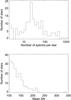Fig. 1 Upper panel: distribution of the number of spectra per star. Lower panel: distribution of the average S/N per star.

We have extracted 167 stars, grouped into six samples from the HARPS survey described in Sousa et al. (2008), and covering the spectral types G0, G2, G5, G8, K0, and K2. The spectral types have been extracted from the Simbad database at the CDS¹. This survey was biased against very active and young stars, and focuses on stars with vsini lower than 3–4 km s^-1, as pointed out by Lovis et al. (2011) in the study of cycles in stars from the same survey.

The spectra have been retrieved from the ESO archive²: We analyse 1D spectra produced by the ESO Data Reduction Software after the interpolation of the 2D echelle spectra (one spectrum per order) over a grid with a constant step in wavelength (0.01 Å). The original 2D spectra are also retrieved for the computation of the uncertainties.

We only retained spectra with a S/N, averaged over all orders, larger than 100. Stars with less than three such spectra were eliminated. Indeed Landstreet (2007) insists on the need to consider only high S/N spectra for this type of analysis, especially if a small number of lines is considered. Although the S/N does not seem to bias our results, low S/N values lead to a large dispersion, which increases the uncertainties and decreases the number of spectral lines which can be analysed, hence the necessity for our threshold. Figure 1 shows the distribution of the number of spectra per star and the average S/N per star. For most stars, we analysed between 10 and 100 spectra, the number ranging between 3 and more than 1000. The S/N values typically lie between 100 and 200.

Figure 2 shows the luminosity versus T_eff for our six samples, provided by Sousa et al. (2008). The global properties of each of these samples are shown in Table 1. The B−V values have been retrieved from the CDS. The individual values for each star are indicated in Table 3.

2.2. Spectra correction and line identification

2.2.1. Continuum correction

We first normalised the spectra for the continuum in two steps: we first identified an upper envelope for each spectrum and then applied a correction factor, to take into account the fact that due the presence of noise the actual continuum is slightly lower than this upper envelope. The procedure is described in Appendix A. We estimated that the resulting uncertainties on the intensities were usually lower than 1%, and much better at high S/N.

2.2.2. Line identification

We used a list of spectral lines of Ca, TiI, TiII, and FeII lines (Dravins 2008), and FeI lines (Nave et al. 1994). Only some of these were selected for the final analysis (see Sect. 2.3). The lines were identified on each spectrum as local minima (over 41 pixels) below a flux equal to 90% of the continuum. Note that for the purpose of line identification, we shift the spectra towards a zero shift position (with a one pixel of 0.01 Å precision) to ensure that the position of the minimum is as close as possible to the theoretical wavelength: in practice, this is done manually for one spectrum per spectral type which serves as a reference and all other spectra are shifted to match this reference spectrum. No interpolation is done, as the pixel precision is sufficient for the line identification and it does not affect the following analysis.

Before any computation on the spectral lines, we eliminated blended lines whose wavelengths were very close to each other in our list and by doing a visual inspection. Another selection using automatic criteria was then implemented (see next section).

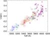Fig. 2 Log of the luminosity (relatively to the solar luminosity) versus temperature (from Sousa et al. 2008) for the main sequence stars in our six samples: G0 (pink stars), G2 (black circles), G5 (yellow triangles), G8 (red squares), K0 (green crosses), and K2 (blue diamonds).

2.3. Differential velocity shifts of spectral lines

To compute the differential velocity shifts of spectral lines, we performed a polynomial fit of the bottom of the line over five pixels (covering a range of 0.04 Å, i.e. corresponding to about 40% of the typical line width at half maximum). We then estimated the position of the minimum of the fit and by comparison with the laboratory wavelength, computed the velocity of the line. For each line we therefore derived a wavelength and its uncertainty, which we then transformed into a radial velocity RV (relative to the laboratory wavelength) and its uncertainty σ_RV. A similar method was also applied by Allende Prieto et al. (2002) and Ramírez et al. (2008). We also derived the flux at the bottom of the line, F, and its uncertainty σ_F. We finally computed the bisector of each line, which was then used for the line selection. We note that in the red part of the optical spectrum, the presence of telluric lines may have impacted a priori our results: this is discussed in Sect. 2.5.

We then selected the lines to be used for our analysis using several automatic criteria on each line. We chose to eliminate: lines with a bisector slope outside the 3σ range of all bisectors (this criteria is close to the one used by Ramírez et al. 2008, but our threshold was not fixed) or a rms of the bisector fit residual outside the 3σ range; lines with a line width outside the 3σ range where σ is deduced from the Gaussian fit of the distribution of the variable.

In most of our computations (especially the slope of RV vs. F) we considered only strong enough lines, that is, points with F lower than 0.6 only, except when indicated otherwise. For selection purposes, we also add a criteria based on the RV – F relationship. For several lines, the RV strongly deviates from the average RV found using the other lines, meaning that such lines could also be blended. We therefore eliminated the lines with measurements outside 5σ (around the linear fit RV versus F). Finally, lines appearing in only one star of the stellar type sample were also eliminated. This allows us to apply a robust criterion on the differential velocity shifts of spectral lines, as described in the following section. The final list of selected lines can be found in Table 4.

2.4. A criterion to characterise the differential velocity shifts of spectral lines

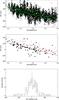Fig. 3 Upper panel: RV versus a normalised flux of the bottom of the lines for HD 223171 (G2), for lines deeper than the 0.6 threshold. Crosses represent individual measurements while green dots correspond to the temporal average for each line. The yellow dots are lines used by Gray (2009). The straight line is a linear fit on the green dots. Middle panel: same as above but showing the wavelength dependence: the black filled circles and solid line are for lines with wavelength below 5750 Å, while the red open circles and dashed lines are for wavelengths above 5750 Å. The green dotted line is the linear fit on all points. Lower panel: distribution of the RV residual after removal of the linear fit, that is, the green dots of the upper panel (solid line). The rms RV is 84 m/s. The dashed line shows the same distribution but for the residual computed after the wavelength-dependence correction (see text), and the rms RV is 78 m/s.

An example of the differential velocity shifts of spectral lines obtained after the line selection described above is shown in Fig. 3 (upper panel) for the G2 star HD 223171. Typical formal uncertainties on RV values after temporally averaging the RV obtained using the same line are in the range 5–15 m/s, while the rms around the linear fit in that example is 84 m/s. 138 lines are used in this example. The average RV computed at each time step over all selected lines has been substracted (the zero is therefore arbitrary here). A correction using the stellar RV provided by the ESO Data Reduction Software does not change our subsequent results significantly.

The dispersion of the residual RV is important. It can be due to several factors, for example: telluric lines, impact of a wavelength dependence, uncertainties on laboratory wavelength (all discussed in Sect. 2.5), impact of blends not taken into account or other properties of the lines, such as the excitation potential (Dravins et al. 1981).

We defined a criterion to easily study the shape of the differential velocity shifts of spectral lines as a function of various parameters: we computed the slope of RV versus F values after averaging all points corresponding to a given line (i.e. typically on the green points in Fig. 3). We note that the formal uncertainties for RV seem to be slightly under-estimated, as estimated by the comparison of the dispersion in RV and F for a given line and the formal uncertainties, by about a factor 1.3 on average but sometime by up to a factor 2: we therefore use the uncertainties derived from the dispersion (of the RV obtained for a given line) to avoid underestimating our uncertainties. This slope is named hereafter TSS, for “Third Signature Slope”, taking up the term “third signature” proposed by Gray (2009) to name the velocity shifts of spectral lines. An example of the linear fit corresponding to the TSS of HD 223171 is shown in Fig. 3). In the following we focus on the analysis of the TSS computed over all spectra of a given star.

2.5. Sources of dispersion or biases

2.5.1. Telluric lines

Telluric lines caused by water may impact the line position estimation. Water wavelengths have been extracted from the HITRAN database (Rothman et al. 2013)³. We listed the telluric lines which are within 0.02 Å of the lines used in our analysis. Most of these lines are very weak and are more than one order of magnitude lower than the stronger lines. Out of the 197 final lines used to compute the TSS in our selection, 5.5% have water telluric lines within 0.02 Å and the percentage decreases to 3% when only considering lines that are used in all six samples (i.e. lines that are most likely to highly impact the TSS estimations). The residual of RV versus F after substracting the linear fit (used to determine the TSS) is not correlated with the position of telluric lines nor with their amplitude. We therefore estimate that the impact on our results should be negligable.

2.5.2. Wavelength dependence

Figure 3 shows the RV versus depth for two different wavelength ranges for HD 223171. There is a clear shift between the two sets of points; lines at shorter wavelengths tending to show larger blueshifts. We observe this effect on most of our stars as well as for the Sun. Note that the difference between the average RV of the black and red dots on the figure is of the order of 10 m/s only, while the shift in RV between the two straight lines is one order of magnitude larger. Such an effect has already been identified by Dravins et al. (1981) and later by Hamilton & Lester (1999), using 298 FeI lines, and for the Sun in both cases. This effect is usually neglected in stellar studies (Allende Prieto et al. 2002) or not relevant because of the small wavelength coverage (Gray 2009) but could explain some differences we observe with the differential velocity shift of Gray (2009), in particular the difference in shape which may be a wavelength effect and the much larger dispersion when considering more lines.

We measured this effect for a large sample of stars for the first time. To quantity this effect, we proceeded as follows: we considered a simple linear relationship between wavelength and RV and substracted from the RV values a factor equal to p_λ × λ, where p_λ is fitted to obtain a minimal rms of the RV residual after the wavelength- and depth- dependance correction. The rms being extremely sensitive to outliers, we performed this computation 100 times for half of the measurements only (which were picked up randomly in the original data set), which also allowed us to derive uncertainties. We then considered the average of the 100 values to estimate p_λ and derive the uncertainties from the distribution of the values. We find values of p_λ between –0.05 and 0.011 m/s/Å typically. The amplitude is compatible with the results of Dravins et al. (1981) and Hamilton & Lester (1999) for the Sun. We conduct a detailed analysis of this effect in Sect. 3.3.

2.5.3. Wavelength uncertainties

As pointed out by Dravins (2008), laboratory wavelength uncertainties have a strong impact on RV determination. The FeII and TiI laboratory wavelengths we used in this work may lead to imprecisions of the order of 6 m/s at, for example, 5000 Å, which is small compared to the observed dispersion. However, most of the FeI wavelength uncertainties are probably one order of magnitude larger and may account for some of the observed dispersion (Nave et al. 1994; Hamilton & Lester 1999). For the example shown in Fig. 3, the quadratic difference between the rms of the residuals for the two categories is 62 m/s.

2.6. Activity level

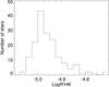Fig. 4 Distribution of the Log ${\mathit{R}}_{\mathrm{HK}}^{\mathrm{\prime }}$ values in our sample (one average per star).

The activity level for each epoch computed using the classical Log ${\mathit{R}}_{\mathrm{HK}}^{\mathrm{\prime }}$ derived from the flux in the Ca II H and K lines, gives the Log of the chromospheric emission. Our values have been corrected using the HARPS-Mt Wilson correcting factor of Lovis et al. (2011). We did not introduce any correction for the thorium leaks, but we estimate that this should not impact our results significantly since we have selected spectra with a good signal to noise ratio and therefore with a large incoming flux. We have not taken into account the metallicity effect either. The distribution of the Log ${\mathit{R}}_{\mathrm{HK}}^{\mathrm{\prime }}$ values (averaged for each star) is shown in Fig. 4.

Lovis et al. (2011) studied 131 of the same stars included in our sample and there is a good correlation between the two estimates of Log ${\mathit{R}}_{\mathrm{HK}}^{\mathrm{\prime }}$. Our computation leads to values approximately 0.5% smaller (i.e.a difference of the order of 0.025) than those derived by Lovis et al. (2011). This difference is not due to the difference in temporal coverage. Our Log ${\mathit{R}}_{\mathrm{HK}}^{\mathrm{\prime }}$ could be slightly biased due to the presence of thorium leaks or to the different spectrum selection, as well as to different B−V values. Nevertheless, this does not impact our conclusion.

2.7. Analysis

The analysis performed in Sect. 3 allows us to study the dependence of the TSS on both the spectral type (or B−V/T_eff) and on the activity level. The TSS and averaged Log ${\mathit{R}}_{\mathrm{HK}}^{\mathrm{\prime }}$ values for each star are shown in Table 3. For each spectral type, we compute the slope of the TSS versus Log ${\mathit{R}}_{\mathrm{HK}}^{\mathrm{\prime }}$.

In a second part of the analysis (Sects. 4 and 5), we use the TSS to derive an average convective blueshift for each star. We consider the Sun as a reference, using the solar spectra obtained by Kurucz et al. (1984) and reduced in 2005 by Kurucz⁴. This allows us to derive RV temporal variations for each star following different assumptions, which may be compared to the actual RV variations.

3. Analysis of the differential velocity shifts of spectral lines

3.1. Dependence on B – V and T_eff

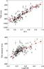Fig. 5 Upper panel: TSS (slope of the differential velocity shifts of spectral lines, in m/s/(F/Fc)) versus the B−V of the stars. The solid line indicates a linear fit while the red dots correspond to TSS averaged over bins in B−V. Lower panel: residual of the TSS after correction of the B−V dependence versus Log ${\mathit{R}}_{\mathrm{HK}}^{\mathrm{\prime }}$. The solid line is a linear fit to the TSS.

The upper panel of Fig. 5 show the TSS versus B−V. The TSS charaterises the slope of the differential velocity shifts of spectral lines and is strongly correlated with B−V (coefficient of 0.88, also meaning a strong anti-correlation with T_eff). If we extrapolate the TSS towards larger B−V (smaller T_eff), it reaches zero for B−V = 1.04 (and T_eff = 4680 K). Figure 5 also shows the TSS averaged over bins in B−V: there may be a trend for a saturation of the TSS at low B−V, but this would need to be confirmed with a study of more massive stars.

3.2. Dependence on activity

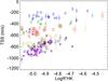Fig. 6 TSS (slope of the differential velocity shifts of spectral lines, in m/s/(F/Fc)) versus Log ${\mathit{R}}_{\mathrm{HK}}^{\mathrm{\prime }}$ for all stars in each sample (same colour and symbol codes as in Fig. 2).

Figure 6 shows the TSS versus Log ${\mathit{R}}_{\mathrm{HK}}^{\mathrm{\prime }}$ for all stars, colour–coded depending on their spectral types. We observe that for a given Log ${\mathit{R}}_{\mathrm{HK}}^{\mathrm{\prime }}$, |TSS| is above a minimal value which decreases as the activity level increases. This minimum value is around 1000 m/s/(F/Fc) (in the following the TSS is in m/s/(F/Fc) where F/Fc represents the flux normalised to the continuum) for the less active stars, and then decreases towards a few hundred m/s/(F/Fc) for the most active stars in our sample.

After substraction of the B−V dependency derived in the previous section (using a linear fit), the TSS residuals are shown on the lower panel of Fig. 5. These residuals are correlated with Log ${\mathit{R}}_{\mathrm{HK}}^{\mathrm{\prime }}$ (coefficient of 0.63), with a slope of 540 ± 30 m/s/(F/Fc). After correction of this Log ${\mathit{R}}_{\mathrm{HK}}^{\mathrm{\prime }}$ dependency, the rms on the TSS residuals is about 80 m/s/(F/Fc). It is still larger than the formal errors on the individual TSS values (estimated when performing the linear fit to compute the TSS and based on the RV and F uncertainties) by a factor of a few units, however, showing that other effects influence the TSS.

For Log ${\mathit{R}}_{\mathrm{HK}}^{\mathrm{\prime }}$ lower than ~–4.85, the slope of the residual TSS versus Log ${\mathit{R}}_{\mathrm{HK}}^{\mathrm{\prime }}$ is probably larger than the global slope, while for more active stars the trend may not be as significant: there could be in fact two regimes, one in which the TSS is very dependent on the activity level (for the less active stars, with a slope of 872 ± 39 m/s/(F/Fc)), and one in which the TSS is less dependent on activity (with a slope of 519 ± 78 m/s/(F/Fc)), suggesting different properties of the magnetic fields. Note that in this description the Sun would be at the edge of the non-active star domain with Log ${\mathit{R}}_{\mathrm{HK}}^{\mathrm{\prime }}$ values between –4.95 and –4.85.

We have noted in Sect. 2.6 that our Log ${\mathit{R}}_{\mathrm{HK}}^{\mathrm{\prime }}$ values were slightly smaller than those of Lovis et al. (2011), by approximately 0.5%, with a large dispersion. This may impact the slope TSS (or TSS residuals) versus Log ${\mathit{R}}_{\mathrm{HK}}^{\mathrm{\prime }}$. A difference of 0.5% impacts the slope with the same amplitude. If we recompute these slopes for each star sample, when there remains enough stars in common, we find larger slopes with differences between 0.5 and 20% (although the number of stars is smaller): our conclusions are therefore not significantly affected by this possible discrepancy.

3.3. Dependence on wavelength

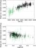Fig. 7 Upper panel: slope of the wavelength dependence factor pλ of the differential velocity shifts versus Teff for G (black stars) and K (green diamonds) stars. The solar value of pλ is 0.124 and is shown as a red circle. Lower panel: same for the pλ residuals after correction of the Teff relationship versus Log ${\mathit{R}}_{\mathrm{HK}}^{\mathrm{\prime }}$.

Figure 7 shows the p_λ factor defined in Sect. 2.5.3 versus the TSS and T_eff for our star sample. p_λ characterises the amplitude of the dependency of differential velocity shifts on the wavelength. We find a strong correlation between this factor and the amplitude of the TSS and with T_eff, at least for T_eff larger than 5400 K. The dispersion is, however, quite large for low T_eff, which may be due to the very small signal in that domain. p_λ is equal to 0.124 m/s/Å for the solar spectrum: this solar value is compatible with the results in Fig. 7 since it is very close to the values obtained for stars at the same T_eff. The impact of this effect on the TSS is significant: for example it decreases from –863 m/s/(F/Fc) to –1163 m/s/(F/Fc) for HD 223171 and from –799 m/s/(F/Fc) to –1107 m/s/(F/Fc) for the Sun.

Finally, we substract the T_eff dependence from p_λ and show the residuals versus Log ${\mathit{R}}_{\mathrm{HK}}^{\mathrm{\prime }}$ in Fig. 7 (lower panel). The rms of the residuals is 0.017 m/s/Å. We find that the activity level impacts the maximum value which can be taken by the slope so that high activity levels reduce the wavelength dependence, at least for G stars.

Both the T_eff and the Log ${\mathit{R}}_{\mathrm{HK}}^{\mathrm{\prime }}$ impacts on p_λ represent strong constraints for the simulation of stellar convection over a large grid of stars, with or without magnetic fields. The wavelength dependence is likely to be due to the stronger contrast of granulation towards lower wavelengths, reinforcing the convective blueshift. This interpretation agrees with our observed trends as a function of T_eff and activity, and such measurements may provide constraints on granulation contrasts.

3.4. Analysis for each spectral type

Fig. 8 Upper panel: TSS (slope of the differential velocity shifts of spectral lines, in m/s/(F/Fc)) averaged for each sample versus the average temperature of the sample (red filled circles and solid line). The green curve (open circles and dashed line) shows the TSS after the wavelength dependence correction. Middle panel: same for the slope of the TSS versus Log ${\mathit{R}}_{\mathrm{HK}}^{\mathrm{\prime }}$. Lower panel: same for the ratio between this slope and the TSS. The dotted line is a linear fit on the ratio in red.

The average TSS was computed for each of the six star samples. The results are shown in Table 2, and in Fig. 8 (upper panel). There is a clear decrease of the TSS towards cooler stars, as seen above. The TSS corrected for the wavelength dependence is also shown and appears larger in amplitude but shows a similar trend.

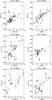Fig. 9 Each panel shows the TSS (slope of the differential velocity shifts of spectral lines, in m/s/(F/Fc)) computed for each star versus the average Log ${\mathit{R}}_{\mathrm{HK}}^{\mathrm{\prime }}$ of that star. The straight line is a linear fit on the measurements.

We now consider the dependence of the TSS on the activity level separately for each spectral type in our sample. The TSS versus the average Log ${\mathit{R}}_{\mathrm{HK}}^{\mathrm{\prime }}$ is shown in Fig. 9, with a positive correlation in all cases. There are however some deviations from the linear fit. This could be due to the fact that the temperatures of the stars vary within a given sample, as well as to inclination effects (see Sect. 4.3 for a discussion). The possible uncertainty in spectral classification could also lead to some dispersion or outliers if some stars are in fact subgiants of luminosity class IV, or have been incorrectly classified. Stellar rotation may also impact our estimates (as discussed for example by Ramírez et al. 2009): after taking into account the fact that both the TSS and the rotation rates vary with spectral type, we find that the TSS residuals do not show any significant trend versus vsini for our sample limited to vsini lower than 5 km s^-1. We do not, therefore, expect a strong bias in this vsini range. On the other hand, we also expect the differential rotation to impact the TSS, as shown by Beeck et al. (2013) for example, and believe that this effect, though difficult to quantify, could add some dispersion.

The slope of the TSS versus the average Log ${\mathit{R}}_{\mathrm{HK}}^{\mathrm{\prime }}$ is shown in Fig. 8 (values are indicated in Table 2) and is smaller for cooler stars while it can be as large as 800 m/s/(F/Fc) for G0 stars. This corresponds to an amplitude of 80 m/s/(F/Fc) for an amplitude of 0.1 of the Log ${\mathit{R}}_{\mathrm{HK}}^{\mathrm{\prime }}$ (i.e. a typical difference in Log ${\mathit{R}}_{\mathrm{HK}}^{\mathrm{\prime }}$ between solar cycle minimum and maximum). An extrapolation of the slope with T_eff gives a zero TSS for T_eff = 4830 K, which is close to the values derived for the TSS.

Finally, the ratio between this slope and the TSS (i.e. between the curves from panels 1 and 2 of Fig. 8) is shown on the lower panel: this ratio, showing the attenuation factor of the convective blueshift due to activity, does not show any strong trend, suggesting that stars of different types probably have a very similar response to magnetic activity relative to the amplitude of convection, that is, the convection may be reduced within the same proportions.

We can compare this last result with the simulations made by Beeck et al. (2015). Their hydrodynamic simulation of granulation in the presence of small scale magnetic fields for stars from F3 to M2 shows a magnetic field strength independant from the spectral type, so that if more flux is available, it is spread over a larger surface. Such a behaviour has also been observed by Steiner et al. (2014) on a small range of simulation parameters. In such conditions we would expect the response in terms of granulation properties (and hence the convective blueshift) to be similar from one spectral type to another, since the magnetic field properties do not change much, which is what we observe.

4. Convective blueshifts

In Sect. 1 we mentioned two related effects of convection on spectral line shifts: the absolute convective shift, which is relevant for the exoplanet RV analysis for example (RV typically computed over all available spectral lines), but difficult to measure directly, and the differential shifts measured in the previous section. To derive the former from differential shift measurements such as the TSS, we need to make some assumptions and use the Sun as a reference.

4.1. Computed convective blueshifts

In this section, we use the TSS computed for each star to estimate its convective blueshift, using two principles:

• We use the assumption made by Gray (2009) thatthe shape of the differential shift of spectral lines is representativeof the absolute convective blueshift due to granulation that weare interested in. In this same publication this factor is computedbetween the curve for a given star and the solar curve used as areference, and is also used to derive the intrinsic radial veloc-ity of these stars: their results show a proportionality betweenthe shape, or in our case the slope, and the absolute convectiveblueshift. In principle it would be possible to check such an as-sumption with output from numerical simulations such as thoseprovided by Ramírez et al. (2009)for K stars or by Magic et al. (2014)for a larger range of stellar parameters, since they compute shiftsfrom a large set of spectral lines leading to both differential andabsolute values. Unfortunately, however, they do not attempt tocheck that assumption.

• We use the Sun as a reference. For that purpose, we need two solar values: the solar TSS_⊙ and the convective blueshift RV_{convbl ⊙}. We derive the solar TSS_⊙ from the solar spectrum of Kurucz et al. (1984) using the set of lines we used for the G2 sample. However, the spectral resolution of this spectrum is 500 000, that is, approximately four times larger than the resolution of HARPS spectra (approx. 120 000): Hamilton & Lester (1999) pointed out that a degraded resolution has a significant impact on slopes such as the TSS we derive for resolution below 200 000, leading to smaller slopes (approx. 25% for the HARPS resolution). We have therefore also computed TSS_⊙ on a degraded solar spectrum, which leads to TSS_⊙ = −776 m/s/(F/Fc) (the difference with the original value being smaller than what was derived by Hamilton & Lester 1999). We use the value of –776 m/s/(F/Fc) in the following. As for the solar convective blueshift, a value of 300 m/s (Dravins 1999) is often used (for example in Meunier et al. 2010b). It corresponds to the values measured over all lines taken into account in classical RV computations such those commonly performed. This estimation is however uncertain, for example due to uncertainties in laboratory wavelengths. Reiners et al. (2016) have recently reevaluated an absolute RV versus spectral line depth for the Sun (i.e. similar to what we have done in Sect. 3 but for absolute- rather than relative RV). Unfortunately, they do not provide the average convective blueshift that corresponds to their results. Using their relationship between the absolute RV and line depth, and a sample of spectral lines we extract from the solar spectrum of Kurucz et al. (1984) for depths between 0.05 and 0.95 and wavelengths between 4000 and 6600 Å, we obtain an average convective blueshift of 435 m/s (i.e. larger than the previous value of 300 m/s). If we assume that when computing the RV using cross-correlations between spectra, the RV is more sensitive to deep lines (we assume a weighting factor equal to the line depth), we obtain a convective blueshift of 355 m/s. In the following we consider this the value to compute the convective blueshift. It should be multiplied by 1.22 if we wish to consider a convective blueshift based on average-between-spectral-line positions rather than a weighted one.

The convective blueshift of each star is therefore computed as follows: ${\mathrm{RV}}_{\mathrm{convbl}}\mathrm{=}\mathrm{TSS}\mathrm{\times }{\mathrm{RV}}_{\mathrm{convbl}\mathrm{\odot }}\mathit{/}{\mathrm{TSS}}_{\mathrm{\odot }}\mathit{,}$(1)where TSS is the stellar value derived in Sect. 3 and the solar values are as discussed above. Figure 10 shows the resulting convective blueshifts for all stars in our sample versus T_eff. There is naturally a strong correlation since our convective blueshift is proportionnal to the TSS. There may also be a plateau for T_eff larger than 5800 K. Note that the convective blueshifts derived from the TSS corrected for the wavelength effect (not represented on the figure) are only 38 m/s lower than the original ones, so the effect is small.

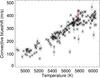Fig. 10 Reconstructed convective blueshift versus Teff for all stars in our sample. The vertical red line corresponds to the solar convective blueshift derived from Reiners et al. (2016) for no weighting and for a weighting equal to the line depth.

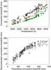Fig. 11 Upper panel: reconstructed convective blueshift versus Teff for the stars for which the formula of Allende Prieto et al. (2013) could be applied (stars). The convective blueshift derived from Allende Prieto et al. (2013) for those stars is shown before correction from the wavelength range (red circle) and after correction (green dots). Lower panel: reconstructed convective blueshift versus those derived from Allende Prieto et al. (2013), from the original TSS (stars) and those corrected for the wavelength dependence (diamonds).

4.2. Comparison of the adopted convective blueshift with theoretical results

We now wish to compare our computed values with theoretical results.

Allende Prieto et al. (2013) performed hydrodynamical simulations of granulation for various star parameters to deduce a number of properties for the exploitation of Gaia observations, including a numerical expression of the convective blueshift of stars depending on their T_eff, log g and metallicity. The formula only being valid for certain ranges in parameters, we have only been able to apply their formula to 93 stars in our sample. The red dots in Fig. 11 represent the theoretical convective blueshift for these stars based on the stellar parameters of Sousa et al. (2008), while our estimation is represented by the black stars. This convective blueshift corresponds to the Gaia wavelength range, that is, 8470–8740 Å. If we compute the solar convective blueshift from the results of Reiners et al. (2016) as above but selecting only lines in this wavelength range, we obtain 459 m/s (computation with line depth weighting) instead of the 355 m/s obtained above. Therefore, to be representative of a large wavelength range RV computation, this theoretical convective blueshift should be divided by 1.29, as shown by the green dots. On the other hand, applying the formula of Allende Prieto et al. (2013) to the solar parameters leads to a convective blueshift of 285 m/s, which is significantly smaller than 459 m/s deduced from the observation of Reiners et al. (2016) for the same wavelength range suggesting that the numerical simulations produce a convection significantly weaker (by a factor of approximately 1.7 below 5800 K) than that observed.

When comparing the simulated convective blueshift (green dots) with the estimated convective blueshift based on the assumption of Sect. 4.1, we naturally find a significant difference in amplitude as well, since the Sun was used as a reference. That said, the trend for T_eff lower than 5800 K is similar, except for the multiplying factor (a factor of approximately 2). Above 5800 K, the trend seems different, with a strong increase observed in the simulation but not in our observations: this will need to be investigated in the future.

Magic et al. (2014) also provide line shifts versus T_eff from numerical simulations of stellar convection as well, with a similar trend in T_eff. Their line shifts are approximately 100 m/s at 5000 K (similar to our values) but in the range 700–800 m/s at 6000 K, that is, slightly larger than our values and much larger than those of Allende Prieto et al. (2013). This could be due to the fact that their line shifts are computed from the bottom of the line (and not for the whole line, as is assumed in the convective blueshift definition here), and/or may correspond to the specific fictitious Fe I line they are using meaning that a direct comparison of the amplitudes is difficult. An interesting feature observed by Magic et al. (2014) however is a saturation appearing at temperatures larger than 6000 K, which may be similar to what we observe.

5. RV variability

We now wish to compare the observed RV variability (derived in Sect. 5.1) with those which can be predicted using our estimated TSS (in Sect. 5.2). We have thus retrieved the radial velocities computed by the ESO Data Reduction Software from the headers of the archive files. These RV must be corrected for two effects:

• 36 stars in our sample bear planets according to the ExtrasolarPlanets Encyclopaedia⁵. We therefore re-trieved the exoplanet parameters, fitted the parameters when notpublished (this is sometimes the case for the time at periastron andperiastron argument), reconstructed the corresponding RV timeseries, and finally substracted the planetary signal from the mea-sured RV. Note that some of these stars bear several planets (22with 1 planet, 9 with 2 planets,3 with 3 planets and 1 with4 planets). One of them has not been correctedbecause the three planets are all below 1 m/s. This isa necessary step, otherwise the induced RV is overestimated andin some cases possible correlation with the Log ${\mathit{R}}_{\mathrm{HK}}^{\mathrm{\prime }}$may be masked by the presence of the planetary signal. In mostcases the parameters have been retrieved from the compilationmade by Mayor et al. (2011).Others were taken from elsewhere (Butleret al. 2006; Naefet al. 2007; Pepeet al. 2011; Hinkelet al. 2015; Díazet al. 2016), and parameters notprovided have been fitted on our time series.

• A very strong RV trend with time is exhibited by six particular stars suggesting the presence of a binary. We have removed the trend before analysing their RV (using a linear fit or a second degree polynomial fit).

5.1. Observed RV versus Log R′_HK

When only considering stars with at least 10 observations (131 stars), 40% of the stars have a correlation between RV Log ${\mathit{R}}_{\mathrm{HK}}^{\mathrm{\prime }}$ above 0.4 and 24% above 0.6. To compute long-term amplitudes, we averaged the RV values in 50 day bins. We made sure to have at least 5 points in each bin (otherwise the observation was discarded) and considered stars with at least 4 such bins in the following analyses. This reduced our sample to 43 stars. From these time series we computed the RV amplitude (defined as the maximum minus the minimum of the binned time series), ΔRV_obs, as well as ΔLog ${\mathit{R}}_{\mathrm{HK}}^{\mathrm{\prime }}$ and the average Log ${\mathit{R}}_{\mathrm{HK}}^{\mathrm{\prime }}$ for comparison purposes. ΔR_obs is compared in the next section with RV variations derived from the convective blueshift. Considering stars with more bins considerably reduces the sample, although the statistics, in terms of stars with a good correlation between RV and Log ${\mathit{R}}_{\mathrm{HK}}^{\mathrm{\prime }}$, are relatively robust: 40% of the stars have a correlation between RV and Log ${\mathit{R}}_{\mathrm{HK}}^{\mathrm{\prime }}$ (from the binned series). The uncertainties on each RV measurement as computed by the ESO Data reduction Software are between 0.2 and 0.6 m/s depending on the star. Because there is also some stellar intrinsic variability and since some bins contain as few as five points, the uncertainties on ΔRV are larger, typically of the order of 1−2 m/s.

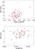Fig. 12 Upper panel: ΔRVobs versus the average Log ${\mathit{R}}_{\mathrm{HK}}^{\mathrm{\prime }}$, computed on the binned time series and for the 43 stars with more than two bins (see text), for G (red stars) and K (green diamonds) stars. Lower panel: same versus ΔLog ${\mathit{R}}_{\mathrm{HK}}^{\mathrm{\prime }}$.

Figure 12 shows ΔRV_obs versus the averaged Log ${\mathit{R}}_{\mathrm{HK}}^{\mathrm{\prime }}$ for each of the 43 stars (which shows no particular trend) and versus the amplitude of the Log ${\mathit{R}}_{\mathrm{HK}}^{\mathrm{\prime }}$. We see that strong variations in RV tend to be associated with stronger amplitudes in Log ${\mathit{R}}_{\mathrm{HK}}^{\mathrm{\prime }}$, although there is a large dispersion.

Our results can be compared with previous RV variations published in the literature. Most of the time only the rms of RV (before binning) versus the average of the Log ${\mathit{R}}_{\mathrm{HK}}^{\mathrm{\prime }}$ or ${\mathit{R}}_{\mathrm{HK}}^{\mathrm{\prime }}$ (and not the amplitude, which we believe is more relevant) is available. Our rms RV falls well within the range of variation of Wright (2005) and Isaacson & Fischer (2010), although we also observe stars with smaller rms. Furthermore, we find, as they do, that there is no clear trend when considering the rms versus the average ${\mathit{R}}_{\mathrm{HK}}^{\mathrm{\prime }}$. This is different from the results of Santos et al. (2000) and Saar et al. (1998), who found larger rms and a trend. We have also computed the slope of ${\mathit{R}}_{\mathrm{HK}}^{\mathrm{\prime }}$ versus RV (before binning) as studied by Lovis et al. (2011) as a function of T_eff. Our slopes are of similar amplitudes in the different T_eff domains.

The Sun, with an amplitude of log ${\mathit{R}}_{\mathrm{HK}}^{\mathrm{\prime }}$ of 0.1 and a predicted amplitude in RV of 8 m/s (Meunier et al. 2010a) falls within the range of values found for our sample.

5.2. Simulated RV

5.2.1. Computation of the simulated RV

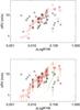Fig. 13 Upper panel: ΔRVobs versus the amplitude of the Log ${\mathit{R}}_{\mathrm{HK}}^{\mathrm{\prime }}$, on averaged time series (see text), in black. ΔRVconv is shown in red. Lower panel: same as the upper panel. Red vertical lines correspond to the ΔRVconv reconstructed for inclinations of the rotational axis in the range 10–90°. The green circle is the solar value (seen equator-on), and the green line indicates what the solar value would be for various inclinations. The orange dashed line corresponds to ΔRVconv reconstructed from Eq. (5) for Teff between 4950 K (lower curve) and 6150 K (higher curve) with a step of 200 K between each curve.

We now estimate the RV variations that would be due to the attenuation of the convective blueshift from the typical dependence of the convective blueshift on activity and from the amplitude of variation of the log ${\mathit{R}}_{\mathrm{HK}}^{\mathrm{\prime }}$ for each star. For a given spectral type, we defined in Sect. 3.4 the slope of the TSS versus Log ${\mathit{R}}_{\mathrm{HK}}^{\mathrm{\prime }}$, hereafter referred to as G. Hence, if a certain star activity level varies with ΔLog ${\mathit{R}}_{\mathrm{HK}\mathrm{◦}}^{\mathrm{\prime }}$ then we expect a variation of ΔTSS_◦ of the TSS, the ratio being the slope: $\mathit{G}\mathrm{=}\mathrm{\Delta }{\mathrm{TSS}}_{\mathrm{◦}}\mathit{/}\mathrm{\Delta }\mathrm{Log}\hspace{0.17em}{\mathit{R}}_{\mathrm{HK}\mathrm{◦}}^{\mathrm{\prime }}\mathit{.}$(2)For this star, following Eq. (1), the convective blueshift is: ${\mathrm{RV}}_{\mathrm{convbl}\mathrm{◦}}\mathrm{=}{\mathrm{TSS}}_{\mathrm{◦}}\mathrm{\times }{\mathrm{RV}}_{\mathrm{convbl}\mathrm{\odot }}\mathit{/}\mathrm{TS}{\mathrm{S}}_{\mathrm{\odot }}\mathit{.}$(3)As a consequence, for any star we study with the same temperature (i.e. corresponding to the same G) and with an observed variability of ΔLog ${\mathit{R}}_{\mathrm{HK}\mathrm{\ast }}^{\mathrm{\prime }}$, we expect the TSS to vary by: $\mathrm{\Delta }{\mathrm{TSS}}_{\mathrm{\ast }}\mathrm{=}\mathit{G}\mathrm{\times }\mathrm{\Delta }\mathrm{Log}\hspace{0.17em}{\mathit{R}}_{\mathrm{HK}\mathrm{\ast }}^{\mathrm{\prime }}\mathit{.}$(4)In the following, G will be interpolated for each T_eff from the curve in Fig. 8. From Eqs. (1) and (4), the variation of the convective blueshift with time (i.e. the RV variation due to the attenuation of the convective blueshift) is: $\mathrm{\Delta }{\mathrm{RV}}_{\mathrm{conv}}\mathrm{=}\mathit{G}\mathrm{\times }{\mathrm{RV}}_{\mathrm{convbl}\mathrm{\odot }}\mathit{/}\mathrm{TS}{\mathrm{S}}_{\mathrm{\odot }}\mathrm{\Delta }\mathrm{Log}\hspace{0.17em}{\mathit{R}}_{\mathrm{HK}}^{\mathrm{\prime }}\mathit{.}$(5)ΔRV_conv is then compared with ΔRV_obs (derived in Sect. 5.1) and plotted as a function of ΔLog ${\mathit{R}}_{\mathrm{HK}}^{\mathrm{\prime }}$ in Fig. 13 (upper panel). The global amplitude corresponds to observations. We note that ΔRV_conv is not correlated with ΔRV_obs however, although the amplitudes are compatible, meaning that for a given star the reconstructed value can be quite different from the observed one. This could be due to the fact that Eq. (5) does not include any dependence on inclination of the stellar rotational axis and therefore we assume in the following that it corresponds to an inclination of 45°, as the slope G for a given spectral type has been computed for a sample of stars with various random inclinations.

5.2.2. Impact of inclination on the estimation

The way we estimated the impact of inclination is detailed in Appendix B. The results are shown in Fig. 13 (bottom panel) as red lines. When taking into account the impact of inclination on our reconstructed ΔRV_conv, the obtained dispersion and range of values correspond well to the observations. Note that the ranges have been computed assuming solar activity patterns: for a star with a different latitude distribution of magnetic activity (i.e. close to the equator, or on the contrary able to extend more poleward) we expect the laws such as those shown in Fig. B.2 to be slightly different, leading to slightly different ranges. We conclude that a large part of the observed dispersion can be explained by the various inclinations of the stars in our sample.

For comparison purposes, Fig. 13 also shows the curves corresponding to Eq. (5) for seven values of T_eff spanning our sample (orange dashed line), starting with 4950 K (bottom line) and then with increasing T_eff (with a step of 200 K) up to 6150 K. The green circle indicates the position of the Sun, and its track for various inclinations as computed by Borgniet et al. (2015). The Sun is localised at a relatively low position compared to other stars of similar temperature and to the straight line corresponding to 5750 K. However, the stars in our sample which fall within the same T_eff range all exhibit ΔLog ${\mathit{R}}_{\mathrm{HK}}^{\mathrm{\prime }}$ lower than 0.05, therefore it is not straightforward to extrapolate their behaviour for a larger variability such as the one observed for the Sun. We conclude that inclination allows for a large dispersion in RV amplitude for a given activity variability.

6. Conclusion

We have defined a criterion to characterise the differential velocity shift of spectral lines for a sample of 167 main sequence stars with spectral types in the range K2 to G0. We estimate the slope of RV versus the flux F at the bottom of each spectral line (studied by Dravins et al. 1981, for the Sun), which we named the TSS, versus the spectral type, the activity level and wavelength. We focus on temporally averaged properties. Our conclusions are as follows:

• We find a decreasing TSS and therefore a decreasing con-vective blueshift amplitude with decreasing temperature,as expected, with a convective blueshift of approximately150 m/s for K2 stars and 500 m/s forG0 stars. The derived convective blueshift basedon the assumption made by Gray (2009) that theconvective blueshift is proportionnal to the shape (the slope in ourcase) of the differential velocity shifts shows a trend with temper-ature which is a in close agreement with the granulation simula-tions of Allende Prieto et al. (2013)but twice larger in amplitude for temperatures lower than5800 K. There is also a discrepancy in the trendfor the highest temperature (above 5800 K),suggesting further analysis is needed, as there may be a sat-uration effect not visible in the simulation by Allende Prietoet al. (2013) but obtained by Magicet al. (2014).

• We find, for the first time, a significant and strong variation of the TSS (and hence of the convective blueshift) with the average activity level of the star in the K2 to G0 domain.

• The relative variations of the TSS with activity, that is, the slope of the TSS variation with Log ${\mathit{R}}_{\mathrm{HK}}^{\mathrm{\prime }}$ divided by the average TSS for that spectral type, are relatively constant with spectral type. Therefore the TSS variations with activity are proportional to the amplitude of the convective blueshift for all spectral types. A constant attenuation factor is compatible with the MHD simulations performed by Beeck et al. (2015).

• We derive an amplitude of RV variations due to the convective blueshift (including a possible range corresponding to different inclination assumptions) from the estimated convective blueshift and observed Log ${\mathit{R}}_{\mathrm{HK}}^{\mathrm{\prime }}$ variations. This amplitude is compared with the observed RV variations for the stars of our sample. We find a global agreement in term of amplitude. The effects of temperature and inclination (following the inclination study for the Sun of Borgniet et al. 2015) aptly explain the observed dispersion, except in the domain of small activity variability, in which some of our RV amplitudes may be overestimated.

• Dravins et al. (1981) and Hamilton & Lester (1999) showed that, for the Sun, the RV depends on wavelength, clearly visible when taking into account the F dependence. We generalise these results and observe this dependence for the first time for a large sample of main sequence stars. The amplitude of the effect decreases towards smaller temperatures, and disappears for our K2 sample. It also decreases as activity increases.

The results obtained in this paper will allow us to perform realistic simulations of RV temporal series for various types of stars, following the work of Borgniet et al. (2015) for the Sun.

Acknowledgments

This work has been funded by the Université de Grenoble Alpes project called “Alpes Grenoble Innovation Recherche (AGIR)” and by the ANR GIPSE ANR-14-CE33-0018. This work made use of several public archives and databases: The HARPS data have been retrieved from the ESO archive at http://archive.eso.org/wdb/wdb/adp/phase3_spectral/form. This research has made use of the SIMBAD database, operated at CDS, Strasbourg, France. The telluric line properties were retrieved from the HINTRAN database. Exoplanets information was retrieved from the Extrasolar Planet Encyclopaedia at http://exoplanet.eu/. The solar spectrum from Kurucz et al. (1984) is available on-line at http://kurucz.harvard.edu/sun/fluxatlas2005/.

References

Appendix A: Continuum correction: procedure

The procedure is as follows:

• We define an upper envelope for each spectrum by retrieving thehighest intensity in each 5 Å bin. We eliminate outliers that may bedue to cosmics by performing a linear fit on eleven such adjacentpoints and removing the point with the largest residual. For eachremaining point, we recompute the linear fit and consider theresidual after the fit removal at that point. The distribution of thesevalues is fitted with a Gaussian. Points with values outside a 3σrange or too close to each other are also eliminated. The resultingintensities versus wavelength are then smoothed andinterpolated on the original list of wavelengths, providing anupper envelope for the spectrum.

• The spectrum is then divided by this upper envelope. The distribution of all intensities in the spectrum peaks at the level of the continuum (its position depends on the noise level). This provides a correcting factor, by which the spectra is multiplied to provide the final spectra, normalised to a continuum of 1. A visual examination shows that the continuum can be slightly off in a few wavelength ranges. The effect is larger for low S/N spectra.

Note that in principle the correcting factor depends on the wavelength, as the S/N depends on the order. However the impact on our analysis is very limited, especially since we have considered lines in the 5000–6855 Å range only.

Appendix B: Impact of inclination on the RV variability

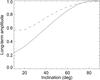Fig. B.1 Dependence of the attenuation of the long-term convective blueshift ΔRVconv versus inclination fRV (solid line), normalised to one, for a solar simulation (from Borgniet et al. 2015), and variation of the corresponding plage coverage fff (dashed line), also normalised.

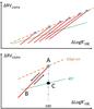Fig. B.2 Upper panel: schematic view of ΔRVconv versus $\mathrm{\Delta }\mathrm{Log}\hspace{0.17em}{\mathit{R}}_{\mathrm{HKobs}}^{\mathrm{\prime }}$ showing the impact of inclination for a star at a given temperature and different activity levels: seen equator-on (orange dashed line with blue stars), at 45° (dotted green line). The red tracks correspond to the various inclinations for each blue star. The vertical dotted-dashed blue thick line corresponds to the various ΔRVconv that would correspond to different inclinations for a given observed $\mathrm{\Delta }\mathrm{Log}\hspace{0.17em}{\mathit{R}}_{\mathrm{HKobs}}^{\mathrm{\prime }}$. Lower panel: same zoomed in on one particular observation (see text).

We now consider the dependence of the rotational axis on inclination. Borgniet et al. (2015) have studied the impact of inclination on the RV time series from a solar simulation for various inclinations. The RV and plage coverage (which is directly related to the chromospheric emission) are maximal for a Sun seen equator-on and minimal for a pole-on configuration. They do not vary by the same factor however: a factor of 4.2 for RV and a factor of 1.8 for the plage coverage. In the following we will apply this RV factor f_RV to our computed RV to derive a reconstructed RV at a given inclination to another. We apply the plage coverage factor f_ff to Log ${\mathit{R}}_{\mathrm{HK}}^{\mathrm{\prime }}$ as well. Normalised f_RV and f_ff are shown in Fig. B.1.

We now estimate the impact of this dependence on our reconstructed ΔRV_conv. Let us first consider a star, with a given T_eff, seen equator-on (as the Sun). Depending on the amplitude of activity variability of this star, it will be located at different positions in the ($\mathrm{\Delta }\mathrm{Log}\hspace{0.17em}{\mathit{R}}_{\mathrm{HK}}^{\mathrm{\prime }}$, ΔRV_conv) diagram, and will follow the orange line in Fig. B.2 (upper panel), different blue stars corresponding to specific $\mathrm{\Delta }\mathrm{Log}\hspace{0.17em}{\mathit{R}}_{\mathrm{HK}}^{\mathrm{\prime }}$. If the same stars were seen with an inclination of 45°, they would be located on the black line, whose slope is defined by G (defined in Sect. 5.2.1, for the T_eff of the star). One of these stars with a given activity level but seen at different inclinations would follow one of the red tracks. When we reconstruct ΔRV_conv as above, we do not know the inclination of the star, only the amplitude of variation of the Log ${\mathit{R}}_{\mathrm{HK}}^{\mathrm{\prime }}$. Given an observed $\mathrm{\Delta }\mathrm{Log}\hspace{0.17em}{\mathit{R}}_{\mathrm{HKobs}}^{\mathrm{\prime }}$, the reconstructed ΔRV_conv for various inclinations should therefore be at any location along the vertical thick blue line (close to the top if seen edge on, and close to the bottom if seen pole-on), that is, where the vertical line crosses any red track.

We therefore wish to compute the values corresponding to this blue segment for each of our stars, to estimate the value it would take for all possible inclinations. Note that our computations are made for inclinations between 10 and 90°; the range covered by the simulation of Borgniet et al. (2015). In Fig. B.2 (lower panel), the black dot at C is the reconstructed ΔRV_conv from Eq. (5) applied to the observed $\mathrm{\Delta }\mathrm{Log}\hspace{0.17em}{\mathit{R}}_{\mathrm{HKobs}}^{\mathrm{\prime }}$. As an example, let us consider how to reconstruct ΔRV_conv for an equator-on configuration, that is, for point A, which has the same observed $\mathrm{\Delta }\mathrm{Log}\hspace{0.17em}{\mathit{R}}_{\mathrm{HKobs}}^{\mathrm{\prime }}$. This star is then on the red track: if it was seen at a different inclination (i.e. from another observer’s point of view) it would be along this track. Such an observer observing it at 45° would therefore see point B, which has the following coordinates: $\mathrm{\Delta }\mathrm{Log}\hspace{0.17em}{\mathit{R}}_{\mathrm{HK}}^{\mathrm{\prime }}\mathrm{\left(}\mathrm{B}\mathrm{\right)}\mathrm{=}\mathrm{\Delta }\mathrm{Log}\hspace{0.17em}{\mathit{R}}_{\mathrm{HKobs}}^{\mathrm{\prime }}\mathrm{\times }{\mathit{f}}_{\mathrm{ff}}\mathrm{\left(}{\mathrm{45}}^{\mathrm{◦}}\mathrm{\right)}\mathit{/}{\mathit{f}}_{\mathrm{ff}}\mathrm{\left(}{\mathrm{90}}^{\mathrm{◦}}\mathrm{\right)}\mathit{.}$(B.1)

ΔRV_conv(B) is derived from Eq. (5) applied to $\mathrm{\Delta }\mathrm{Log}\hspace{0.17em}{\mathit{R}}_{\mathrm{HK}}^{\mathrm{\prime }}$(B). From this point B, we can move along the track back to point A by applying the RV correcting factor to the point B RV amplitude: $\mathrm{\Delta }{\mathrm{RV}}_{\mathrm{conv}}\mathrm{\left(}\mathrm{A}\mathrm{\right)}\mathrm{=}\mathrm{\Delta }{\mathrm{RV}}_{\mathrm{conv}}\mathrm{\left(}\mathrm{B}\mathrm{\right)}\mathrm{\times }{\mathit{f}}_{\mathrm{RV}}\mathrm{\left(}{\mathrm{90}}^{\mathrm{◦}}\mathrm{\right)}\mathit{/}{\mathit{f}}_{\mathrm{RV}}\mathrm{\left(}{\mathrm{45}}^{\mathrm{◦}}\mathrm{\right)}\mathit{.}$(B.2)The same computation, using Eqs. (B.1) and (B.2) but applied to any inclination instead of 90° will provide the range of ΔRV_conv covering all inclinations between 10 and 90°.

All Tables

All Figures

	Fig. 1 Upper panel: distribution of the number of spectra per star. Lower panel: distribution of the average S/N per star.
In the text

	Fig. 2 Log of the luminosity (relatively to the solar luminosity) versus temperature (from Sousa et al. 2008) for the main sequence stars in our six samples: G0 (pink stars), G2 (black circles), G5 (yellow triangles), G8 (red squares), K0 (green crosses), and K2 (blue diamonds).
In the text

Fig. 3 Upper panel: RV versus a normalised flux of the bottom of the lines for HD 223171 (G2), for lines deeper than the 0.6 threshold. Crosses represent individual measurements while green dots correspond to the temporal average for each line. The yellow dots are lines used by Gray (2009). The straight line is a linear fit on the green dots. Middle panel: same as above but showing the wavelength dependence: the black filled circles and solid line are for lines with wavelength below 5750 Å, while the red open circles and dashed lines are for wavelengths above 5750 Å. The green dotted line is the linear fit on all points. Lower panel: distribution of the RV residual after removal of the linear fit, that is, the green dots of the upper panel (solid line). The rms RV is 84 m/s. The dashed line shows the same distribution but for the residual computed after the wavelength-dependence correction (see text), and the rms RV is 78 m/s.

In the text

	Fig. 4 Distribution of the Log ${\mathit{R}}_{\mathrm{HK}}^{\mathrm{\prime }}$ values in our sample (one average per star).
In the text

Fig. 5 Upper panel: TSS (slope of the differential velocity shifts of spectral lines, in m/s/(F/Fc)) versus the B−V of the stars. The solid line indicates a linear fit while the red dots correspond to TSS averaged over bins in B−V. Lower panel: residual of the TSS after correction of the B−V dependence versus Log ${\mathit{R}}_{\mathrm{HK}}^{\mathrm{\prime }}$. The solid line is a linear fit to the TSS.

In the text

	Fig. 6 TSS (slope of the differential velocity shifts of spectral lines, in m/s/(F/Fc)) versus Log ${\mathit{R}}_{\mathrm{HK}}^{\mathrm{\prime }}$ for all stars in each sample (same colour and symbol codes as in Fig. 2).
In the text

	Fig. 7 Upper panel: slope of the wavelength dependence factor pλ of the differential velocity shifts versus Teff for G (black stars) and K (green diamonds) stars. The solar value of pλ is 0.124 and is shown as a red circle. Lower panel: same for the pλ residuals after correction of the Teff relationship versus Log ${\mathit{R}}_{\mathrm{HK}}^{\mathrm{\prime }}$.
In the text

Fig. 8 Upper panel: TSS (slope of the differential velocity shifts of spectral lines, in m/s/(F/Fc)) averaged for each sample versus the average temperature of the sample (red filled circles and solid line). The green curve (open circles and dashed line) shows the TSS after the wavelength dependence correction. Middle panel: same for the slope of the TSS versus Log ${\mathit{R}}_{\mathrm{HK}}^{\mathrm{\prime }}$. Lower panel: same for the ratio between this slope and the TSS. The dotted line is a linear fit on the ratio in red.

In the text

	Fig. 9 Each panel shows the TSS (slope of the differential velocity shifts of spectral lines, in m/s/(F/Fc)) computed for each star versus the average Log ${\mathit{R}}_{\mathrm{HK}}^{\mathrm{\prime }}$ of that star. The straight line is a linear fit on the measurements.
In the text

	Fig. 10 Reconstructed convective blueshift versus Teff for all stars in our sample. The vertical red line corresponds to the solar convective blueshift derived from Reiners et al. (2016) for no weighting and for a weighting equal to the line depth.
In the text

Fig. 11 Upper panel: reconstructed convective blueshift versus Teff for the stars for which the formula of Allende Prieto et al. (2013) could be applied (stars). The convective blueshift derived from Allende Prieto et al. (2013) for those stars is shown before correction from the wavelength range (red circle) and after correction (green dots). Lower panel: reconstructed convective blueshift versus those derived from Allende Prieto et al. (2013), from the original TSS (stars) and those corrected for the wavelength dependence (diamonds).

In the text

	Fig. 12 Upper panel: ΔRVobs versus the average Log ${\mathit{R}}_{\mathrm{HK}}^{\mathrm{\prime }}$, computed on the binned time series and for the 43 stars with more than two bins (see text), for G (red stars) and K (green diamonds) stars. Lower panel: same versus ΔLog ${\mathit{R}}_{\mathrm{HK}}^{\mathrm{\prime }}$.
In the text

Fig. 13 Upper panel: ΔRVobs versus the amplitude of the Log ${\mathit{R}}_{\mathrm{HK}}^{\mathrm{\prime }}$, on averaged time series (see text), in black. ΔRVconv is shown in red. Lower panel: same as the upper panel. Red vertical lines correspond to the ΔRVconv reconstructed for inclinations of the rotational axis in the range 10–90°. The green circle is the solar value (seen equator-on), and the green line indicates what the solar value would be for various inclinations. The orange dashed line corresponds to ΔRVconv reconstructed from Eq. (5) for Teff between 4950 K (lower curve) and 6150 K (higher curve) with a step of 200 K between each curve.

In the text

	Fig. B.1 Dependence of the attenuation of the long-term convective blueshift ΔRVconv versus inclination fRV (solid line), normalised to one, for a solar simulation (from Borgniet et al. 2015), and variation of the corresponding plage coverage fff (dashed line), also normalised.
In the text

Fig. B.2 Upper panel: schematic view of ΔRVconv versus $\mathrm{\Delta }\mathrm{Log}\hspace{0.17em}{\mathit{R}}_{\mathrm{HKobs}}^{\mathrm{\prime }}$ showing the impact of inclination for a star at a given temperature and different activity levels: seen equator-on (orange dashed line with blue stars), at 45° (dotted green line). The red tracks correspond to the various inclinations for each blue star. The vertical dotted-dashed blue thick line corresponds to the various ΔRVconv that would correspond to different inclinations for a given observed $\mathrm{\Delta }\mathrm{Log}\hspace{0.17em}{\mathit{R}}_{\mathrm{HKobs}}^{\mathrm{\prime }}$. Lower panel: same zoomed in on one particular observation (see text).

In the text

References

- Allen de Prieto, C., Lambert, D. L., Tull, R. G., & MacQueen, P. J. 2002, ApJ, 566, L93 [NASA ADS] [CrossRef] [Google Scholar]
- Allen de Prieto, C., Koesterke, L., Ludwig, H.-G., Freytag, B., & Caffau, E. 2013, A&A, 550, A103 [NASA ADS] [CrossRef] [EDP Sciences] [Google Scholar]
- Beeck, B., Cameron, R. H., Reiners, A., & Schüssler, M. 2013, A&A, 558, A49 [NASA ADS] [CrossRef] [EDP Sciences] [Google Scholar]
- Beeck, B., Schüssler, M., Cameron, R. H., & Reiners, A. 2015, A&A, 581, A42 [NASA ADS] [CrossRef] [EDP Sciences] [Google Scholar]
- Borgniet, S., Meunier, N., & Lagrange, A.-M. 2015, A&A, 581, A133 [NASA ADS] [CrossRef] [EDP Sciences] [Google Scholar]
- Brandt, P. N., & Solanki, S. K. 1990, A&A, 231, 221 [NASA ADS] [Google Scholar]
- Butler, R. P., Wright, J. T., Marcy, G. W., et al. 2006, ApJ, 646, 505 [NASA ADS] [CrossRef] [Google Scholar]
- Díaz, R. F., Ségransan, D., Udry, S., et al. 2016, A&A, 585, A134 [NASA ADS] [CrossRef] [EDP Sciences] [Google Scholar]
- Dravins, D. 1987, A&A, 172, 211 [NASA ADS] [Google Scholar]
- Dravins, D. 1999, in Precise Stellar Radial Velocities, IAU Colloq., 170, eds. J. B. Hearnshaw, & C. D. Scarfe, ASP Conf. Ser., 185, 268 [Google Scholar]
- Dravins, D. 2008, A&A, 492, 199 [NASA ADS] [CrossRef] [EDP Sciences] [Google Scholar]
- Dravins, D., & Nordlund, A. 1990, A&A, 228, 203 [NASA ADS] [Google Scholar]
- Dravins, D., Lindegren, L., & Nordlund, A. 1981, A&A, 96, 345 [NASA ADS] [Google Scholar]
- Dumusque, X., Glenday, A., Phillips, D. F., et al. 2015, ApJ, 814, L21 [NASA ADS] [CrossRef] [Google Scholar]
- Gray, D. F. 1982, ApJ, 255, 200 [NASA ADS] [CrossRef] [Google Scholar]
- Gray, D. F. 2009, ApJ, 697, 1032 [NASA ADS] [CrossRef] [Google Scholar]
- Gray, D. F., & Baliunas, S. L. 1994, ApJ, 427, 1042 [NASA ADS] [CrossRef] [Google Scholar]
- Gray, D. F., & Baliunas, S. L. 1995, ApJ, 441, 436 [NASA ADS] [CrossRef] [Google Scholar]
- Gray, D. F., Baliunas, S. L., Lockwood, G. W., & Skiff, B. A. 1992, ApJ, 400, 681 [NASA ADS] [CrossRef] [Google Scholar]
- Gray, D. F., Baliunas, S. L., Lockwood, G. W., & Skiff, B. A. 1996a, ApJ, 465, 945 [NASA ADS] [CrossRef] [Google Scholar]
- Gray, D. F., Baliunas, S. L., Lockwood, G. W., & Skiff, B. A. 1996b, ApJ, 456, 365 [NASA ADS] [CrossRef] [Google Scholar]
- Hamilton, D., & Lester, J. B. 1999, PASP, 111, 1132 [NASA ADS] [CrossRef] [Google Scholar]
- Haywood, R. D., Collier Cameron, A., Unruh, Y. C., et al. 2016, MNRAS, 457, 3637 [NASA ADS] [CrossRef] [Google Scholar]
- Hinkel, N. R., Kane, S. R., Henry, G. W., et al. 2015, ApJ, 803, 8 [NASA ADS] [CrossRef] [Google Scholar]
- Isaacson, H., & Fischer, D. 2010, ApJ, 725, 875 [NASA ADS] [CrossRef] [Google Scholar]
- Kurucz, R. L., Furenlid, I., Brault, J., & Testerman, L. 1984, Solar flux atlas from 296 to 1300 nm (National Solar Observatory) [Google Scholar]
- Landstreet, J. D. 2007, in The Future of Photometric, Spectrophotometric and Polarimetric Standardization, ed. C. Sterken, ASP Conf. Ser., 364, 481 [Google Scholar]
- Lanza, A. F., Molaro, P., Monaco, L., & Haywood, R. D. 2016, A&A, 587, A103 [NASA ADS] [CrossRef] [EDP Sciences] [Google Scholar]
- Lovis, C., Dumusque, X., Santos, N. C., et al. 2011, ArXiv e-prints [arXiv:1107.5325] [Google Scholar]
- Magic, Z., & Asplund, M. 2014, A&A, submitted [arXiv:1405.7628] [Google Scholar]
- Magic, Z., Collet, R., & Asplund, M. 2014, ArXiv e-prints [arXiv:1403.6245] [Google Scholar]
- Magic, Z., Collet, R., Asplund, M., et al. 2013, A&A, 557, A26 [NASA ADS] [CrossRef] [EDP Sciences] [Google Scholar]
- Mayor, M., Marmier, M., Lovis, C., et al. 2011, A&A, submitted [arXiv:1109.2497] [Google Scholar]
- Meunier, N., Desort, M., & Lagrange, A.-M. 2010a, A&A, 512, A39 [NASA ADS] [CrossRef] [EDP Sciences] [Google Scholar]
- Meunier, N., Lagrange, A.-M., & Desort, M. 2010b, A&A, 519, A66 [NASA ADS] [CrossRef] [EDP Sciences] [Google Scholar]
- Naef, D., Mayor, M., Benz, W., et al. 2007, A&A, 470, 721 [NASA ADS] [CrossRef] [EDP Sciences] [Google Scholar]
- Nave, G., Johansson, S., Learner, R. C. M., Thorne, A. P., & Brault, J. W. 1994, ApJS, 94, 221 [NASA ADS] [CrossRef] [Google Scholar]
- Pasquini, L., Melo, C., Chavero, C., et al. 2011, A&A, 526, A127 [NASA ADS] [CrossRef] [EDP Sciences] [Google Scholar]
- Pepe, F., Lovis, C., Ségransan, D., et al. 2011, A&A, 534, A58 [NASA ADS] [CrossRef] [EDP Sciences] [Google Scholar]
- Ramírez, I., Allen de Prieto, C., Koesterke, L., Lambert, D. L., & Asplund, M. 2009, A&A, 501, 1087 [NASA ADS] [CrossRef] [EDP Sciences] [Google Scholar]
- Ramírez, I., Allen de Prieto, C., & Lambert, D. L. 2008, A&A, 492, 841 [NASA ADS] [CrossRef] [EDP Sciences] [Google Scholar]
- Reiners, A., Mrotzek, N., Lemke, U., Hinrichs, J., & Reinsch, K. 2016, A&A, 587, A65 [NASA ADS] [CrossRef] [EDP Sciences] [Google Scholar]
- Rothman, L. S., Gordon, I. E., Babikov, Y., et al. 2013, J. Quant. Spectr. Rad. Transf., 130, 4 [Google Scholar]
- Saar, S. H., Butler, R. P., & Marcy, G. W. 1998, ApJ, 498, L153 [Google Scholar]
- Santos, N. C., Mayor, M., Naef, D., et al. 2000, A&A, 361, 265 [NASA ADS] [Google Scholar]
- Sousa, S. G., Santos, N. C., Mayor, M., et al. 2008, A&A, 487, 373 [NASA ADS] [CrossRef] [EDP Sciences] [MathSciNet] [Google Scholar]
- Steiner, O., Salhab, R., Freytag, B., et al. 2014, PASJ, 66, S5 [NASA ADS] [Google Scholar]
- Trampedach, R., Asplund, M., Collet, R., Nordlund, Å., & Stein, R. F. 2013, ApJ, 769, 18 [NASA ADS] [CrossRef] [Google Scholar]
- Tremblay, P.-E., Ludwig, H.-G., Freytag, B., Steffen, M., & Caffau, E. 2013, A&A, 557, A7 [NASA ADS] [CrossRef] [EDP Sciences] [Google Scholar]
- Wright, J. T. 2005, PASP, 117, 657 [NASA ADS] [CrossRef] [Google Scholar]