| Issue |
A&A
Volume 592, August 2016
|
|
|---|---|---|
| Article Number | A19 | |
| Number of page(s) | 22 | |
| Section | Extragalactic astronomy | |
| DOI | https://doi.org/10.1051/0004-6361/201527772 | |
| Published online | 05 July 2016 | |
Inferring the star-formation histories of the most massive and passive early-type galaxies at z < 0.3
1 Dipartimento di Fisica e Astronomia, Università di Bologna, Viale Berti Pichat 6/2, 40127 Bologna, Italy
e-mail: This email address is being protected from spambots. You need JavaScript enabled to view it.
2 INAF–Osservatorio Astronomico di Bologna, via Ranzani 1, 40127 Bologna, Italy
Received: 17 November 2015
Accepted: 24 April 2016
Abstract
Context. In the Λ cold dark matter (ΛCDM) cosmological framework, massive galaxies are the end-points of the hierarchical evolution and are therefore key probes for understanding how the baryonic matter evolves within the dark matter halos.
Aims. The aim of this work is to use the archaeological approach in order to infer the stellar population properties and star formation histories of the most massive (M > 1010.75 M⊙) and passive early-type galaxies (ETGs) at 0 < z < 0.3 (corresponding to a cosmic time interval of ~3.3 Gyr) based on stacked, high signal-to-noise (S/N), spectra extracted from the Sloan Digital Sky Survey (SDSS). Our study is focused on the most passive ETGs in order to avoid the contamination of galaxies with residual star formation activity and extract the evolutionary information on the oldest envelope of the global galaxy population.
Methods. Unlike most previous studies in this field, we did not rely on individual absorption features such as the Lick indices, but we used the information present in the full spectrum with the STARLIGHT public code, adopting different stellar population synthesis models. Successful tests have been performed to assess the reliability of STARLIGHT to retrieve the evolutionary properties of the ETG stellar populations such as the age, metallicity and star formation history. The results indicate that these properties can be derived with accuracy better than 10% at S/N ≳ 10–20, and also that the procedure of stacking galaxy spectra does not introduce significant biases into their retrieval.
Results. Based on our spectral analysis, we found that the ETGs of our sample are very old systems – the most massive ones are almost as old as the Universe. The stellar metallicities are slightly supersolar, with a mean of Z ~ 0.027 ± 0.002 and Z ~ 0.029 ± 0.0015 (depending on the spectral synthesis models used for the fit) and do not depend on redshift. Dust extinction is very low, with a mean of AV ~ 0.08 ± 0.030 mag and AV ~ 0.16 ± 0.048 mag. The ETGs show an anti-hierarchical evolution (downsizing) where more massive galaxies are older. The SFHs can be approximated with a parametric function of the form SFR(t) ∝ τ− (c + 1)tc exp(−t/τ), with typical short e-folding times of τ ~ 0.6−0.8 Gyr (with a dispersion of ±0.1 Gyr) and c ~ 0.1 (with a dispersion of ±0.05). Based on the reconstructed SFHs, most of the stellar mass (≳75%) was assembled by z ~ 5 and ≲4% of it can be ascribed to stellar populations younger than ~1 Gyr. The inferred SFHs are also used to place constraints on the properties and evolution of the ETG progenitors. In particular, the ETGs of our samples should have formed most stars through a phase of vigorous star formation (SFRs ≳ 350–400 M⊙ yr-1) at z ≳ 4−5 and are quiescent by z ~ 1.5−2. The expected number density of ETG progenitors, their SFRs and contribution to the star formation rate density of the Universe, the location on the star formation main sequence and the required existence of massive quiescent galaxies at z ≲ 2, are compatible with the current observations, although the uncertainties are still large.
Conclusions. Our results represent an attempt to demonstrate quantitatively the evolutionary link between the most massive ETGs at z < 0.3 and the properties of suitable progenitors at high redshifts. Our results also shows that the full-spectrum fitting is a powerful and complementary approach to reconstruct the star formation histories of massive quiescent galaxies.
Key words: galaxies: evolution / galaxies: formation / galaxies: stellar content
© ESO, 2016
1. Introduction
Despite the success of the Λ cold dark matter (ΛCDM) cosmology (Riess et al. 1998; Perlmutter et al. 1999; Parkinson et al. 2012; Planck Collaboration XIII. 2015), the complete understanding of how baryonic matter evolves leading to the formation of present-day galaxies is still unclear. The presence of cold dark matter in the ΛCDM framework implies a bottom-up or hierarchical formation of structures in which the baryonic mass growth is driven by the merging of dark matter halos which progressively assemble more massive galaxies. However, recent studies showed that merging is not the only channel to build galaxies. Depending on the redshift and dark halo mass, the baryonic mass can also gradually grow thanks to filamentary streams of cold gas (T ~ 104 K) capable of penetrating the shock-heated medium in dark matter halos and feeding the forming galaxies (Dekel et al. 2009). The relative importance of these two channels of mass growth as a function of cosmic time is one of the key questions to be answered to explain how protogalaxies evolved into the different types of galaxies that we see today in the Hubble classification.
In this context, elliptical (E) and lenticular (S0) galaxies, collectively called early-type galaxies (ETGs), have always been considered ideal probes to investigate the cosmic history of mass assembly. Indeed, holding the major share of stellar mass in the local Universe (Renzini 2006, and references therein), massive ETGs are supposed to be the endpoints of the hierarchical evolution, thus enclosing fundamental information about the galaxy formation and mass assembly cosmic history. In this regard, several studies attempted to infer the evolutionary properties of massive ETGs at z ~ 0 (archaeological approach), or to observe directly their progenitors at higher redshifts (look-back approach) (see again Renzini 2006, for a review). The results of these studies suggest an empirical evolutionary trend, called downsizing (see Cowie et al. 1996, for its first definition), where massive galaxies formed earlier and faster than lower mass systems.
The downsizing scenario is evident in several cases of galaxy evolution (Fontanot et al. 2009). In the case of ETGs at z ~ 0, one of the first pieces of observational evidence can be referred to the studies of Dressler et al. (1987), Faber et al. (1992) and Worthey et al. (1992), who found more massive elliptical galaxies to be more enriched in α-elements than less massive ones. These works suggested selective mass-losses, different initial mass functions (IMF) and/or different star-formation timescales as possible explanations for the high level of [α/Fe]. Subsequent studies found the same trend of [α/Fe] with mass (Carollo et al. e.g 1993; Davies et al. 1993; Bender et al. 1993; Thomas et al. 2005; 2010; McDermid et al. 2015), leading to the dominant interpretation that in more massive ETGs, the duration of star formation was substantially shorter than in less massive ones, with timescales short enough (e.g. <0.5 Gyr) to avoid the dilution of the α element abundance (produced by Type II supernovae) by the onset of Fe production by Type Ia supernovae. This is considered to be one of the main pieces of evidence for the shortening of star formation. The age of the ETG stellar populations at z ~ 0 also show evidence of downsizing, with more massive objects being older than less massive ones. These results have been derived both in clusters (Thomas et al. 2005, 2010; Nelan et al. 2005) and in the field (Heavens et al. 2004; Jimenez et al. 2007; Panter et al. 2007; see also Renzini 2006). Most of these studies are based on fitting individual spectral features with the Lick/IDS index approach (Burstein et al. 1984; Worthey et al. 1994) which allows us to mitigate the problem of the age-metallicity degeneracy (Graves & Schiavon 2008; Thomas et al. 2005, 2010; Johansson et al. 2012a; Worthey et al. 2013). However, more recently, other approaches based on the full-spectrum fitting have been developed (e.g. STARLIGHT, Cid Fernandes et al. 2005; VESPA, Tojeiro et al. 2009, 2013, and FIREFLY, Wilkinson et al. 2015), and applied to samples of ETGs at z ~ 0 (Jimenez et al. 2007; Conroy et al. 2014; McDermid et al. 2015). The results based on Lick indices are in general quite consistent with those of full spectral fitting within 10−30% (e.g. Conroy et al. 2014) and support the downsizing evolutionary pattern.
In addition to the archaeological constraints, the look-back studies also provide complementary constraints on the evolution of the ETGs. First of all, massive and passive ETGs (M ~ 1011 M⊙) have been unexpectedly discovered in substantial number up to z ~ 3 (e.g. Cimatti et al. 2004; McCarthy et al. 2004; Kriek et al. 2006; Gobat et al. 2012; Whitaker et al. 2013; Onodera et al. 2015; Mendel et al. 2015). For a fixed mass, these ETGs are on average more compact and therefore denser than present-day analogs (Daddi et al. 2005; Cimatti et al. 2008), especially at z> 1.5 (e.g. Cimatti et al. 2012). The mere existence of these massive systems with absent star formation and old stellar ages (~1–3 Gyr) implies that their star formation ceased at z> 2−3 (consistent with the downsizing scenario) and that their formation mechanism was necessarily fast and leading to a rapid assembly of compact and dense systems. It is relevant to recall here that at the time of their first discovery, these massive, passive and old galaxies at z> 1.5 were not expected at all in theoretical models of galaxy formation (Cimatti et al. 2002, 2004).
More constraints also come from the evolutionary trends emerging from statistical samples of ETGs at z> 0.5 and support the downsizing picture. For instance, the evolution of the fundamental plane indicates a decreasing formation redshift (zF) for galaxies with decreasing mass both in clusters and in the field (Treu et al. 2005). Moreover, if compared to the local one, the faint-end of the luminosity function up to z ~ 1 is progressively depopulated towards higher redshift, unlike its high-luminosity end, suggesting again that more massive galaxies assembled their mass earlier than less massive ones (Cimatti et al. 2006). Furthermore, it has been observed that the galaxy number density rapidly increases from z = 0 to z = 1 for M ≲ 1011 M⊙, while the increase is slower for more massive galaxies (Pozzetti et al. 2010; Moresco et al. 2013), starting to show a significant variation only at z ≳ 1 for the most massive systems (M ≳ 1011 M⊙) (Ilbert et al. 2010, see also van Dokkum 2005; 2010; Muzzin et al. 2013).
The physical interpretation of these results on ETG evolution coming from the archaeological and look-back approaches is not trivial in the hierarchial merging scenario of ΛCDM cosmology because the mass downsizing evolution seems anti-hierchical. However, much progress has been made in the last few decades. For instance, the combination of N-body simulations of dark matter halos evolution (Springel et al. 2005; Boylan-Kolchin et al. 2009) with semi-analytic models for galaxy formation (White & Frenk 1991; Kauffmann et al. 1999; Springel et al. 2005; Lu et al. 2011; Benson 2012) have allowed a significant advance. For example, De Lucia et al. (2006) were able to reproduce the age-reduction of elliptical galaxies by invoking AGN feedback to quench the star formation earlier in more massive systems with respect to less massive ones within the standard framework of the hierarchical assembly for stellar mass. The role of AGNs in influencing galaxy evolution and quenching star formation is supported by several observations (Fabian 2012, and references therein; Cimatti et al. 2013; Cicone et al. 2014; Förster Schreiber et al. 2014); however, other models are able to rapidly form ETGs without invoking the AGN feedback (e.g. Naab et al. 2006, 2009; Khochfar & Silk 2006; Johansson et al. 2012b). More recently, Henriques et al. (2013), (2015) found that the early build-up of low mass galaxies predicted by many models could in fact be prevented by assuming that less massive systems reincorporate the gas ejected by supernova-driven winds later than more massive objects. This kind of assumption, although requiring further investigation, would also reproduce the observed mass assembly downsizing. However, despite the improvements on the theoretical side, many questions remain still open and the physics of massive galaxy formation is not fully understood.
The empirical downsizing scenario implies that the star-forming progenitors of massive and passive ETGs should be present at z ≳ 2. Thus, the identification of these proto-ETGs is a crucial test to validate the downsizing picture and to link the evolutionary properties of ETGs inferred at z ~ 0 with those derived directly at higher redshifts with the look-back approach. The current knowledge on ETG precursors is still fragmentary and we lack a coherent picture. However, star-forming systems with different levels of SF activity and sometimes with compact sizes have been identified at z ≳ 2−3 as potential star-forming progenitors of massive ETGs at z ~ 0 (e.g. Daddi et al. 2004; Finkelstein et al. 2013; Williams et al. 2015). An additional piece of information comes from the host galaxies of QSOs at z ≳ 6, which have stellar masses up to M ~ 1011 M⊙ and high metallicity (e.g. Fan et al. 2003), and also from the surprising identification of a significant number of galaxies at z ≳ 4−5, which have stellar masses up to M ~ 1011 M⊙ and already look quiescent at these high redshifts (e.g. Mobasher et al. 2005; Wiklind et al. 2008; Juarez et al. 2009; Brammer et al. 2011; Marsan et al. 2015), although their properties are based on photometric redshifts and SED fitting, since they are too faint for spectroscopic identification. If these galaxies really were ETG analogs at z ≳ 4−5, they would imply that a fraction of massive galaxies formed rapidly at very high redshifts (say z> 5) and with an intense star formation, if they are observed to be already quiescent at z ~ 4−5.
In this work, we apply the archaeological approach to study the properties of a sample of ETGs at 0.02 <z< 0.3, restricting our analysis only to the most extreme systems, that is, to the most massive (M ≳ 5.6 × 10¹⁰ M⊙) and passive objects. The aim is to infer their star-formation histories and place quantitative constraints on their precursors at high redshifts. In particular, instead of relying on the individual spectral features of these galaxies, we exploit the information contained in their full-spectrum, by means of the public code STARLIGHT (Cid Fernandes et al. 2005).
Throughout this work, we adopt a flat ΛCDM cosmology with ΩM = 0.27; H0 = 72 km s-1 Mpc-1. Moreover, we always refer to galaxy stellar masses.
2. Testing STARLIGHT with simulated ETGs spectra
Our work is based on spectral analysis and makes use of the full-spectrum fitting code STARLIGHT1 (Cid Fernandes et al. 2005), which provides a fit to both galaxy spectral continuum and spectral features.
Basically, the best fit model derived by STARLIGHT is obtained from the combination of many SSP spectra defined in user-made libraries. The contribution of each library spectrum to the best fit model is enclosed in the so-called light- and mass-fraction population vectors, which contain, respectively, the light and the mass fractions with which each library model contributes to the best fit spectrum at a reference λ. These population vectors are derived together with the best fit values for both the stellar velocity dispersion (σ) and stellar extinction (AV).
Before applying STARLIGHT to real data, we test its reliability to reproduce the evolutionary properties, such as age, metallicity, star formation histories (SFHs), dust extinction and velocity dispersion of massive and passive galaxies as a function of the signal-to-noise ratio (S/N) of the input spectra. To do this, we simulate spectra with different S/N and known evolutionary and physical properties treating them as STARLIGHT inputs, and then we compare our assumed inputs with the code outputs.
We create an ensemble of simulated spectra from 3500 to 8500 Å with increasing S/N, starting from BC03 (Bruzual & Charlot 2003) theoretical models. These synthetic models are based on the STELIB stellar spectra library (Le Borgne et al. 2003) and assume a Charbrier IMF (Chabrier 2003). They are defined in the wavelength range 3200−9500 Å and have a resolution of ~3 Å, which is similar to the resolution of the SDSS spectra analyzed in the second part of this work (see Sect. 3). We first define an error eλ for each theoretical spectrum by dividing the median flux of the model in the 6500−7000 Å window by a pre-defined grid of S/N (going from 1 to 10 and from 20 to 500 with step of 10); then, we apply the λ-independent eλ to the whole model spectrum, generating Gaussian random numbers within it and thus producing the simulated flux, as illustrated in Fig. 1. We verified that the assumption of a wavelength-independent error is reasonable, since it reproduces the behaviour of the error of individual SDSS spectra, on which we base our subsequent analysis. In particular, within the rest-frame range 3500–7000 Å (used to fit our data, see Sect. 3), the error of SDSS spectra is constant as a function of wavelength, apart from a discontinuity in correspondence of the overlapping of the blue and the red arm of the spectrograph (at ~6000 Å). As a consequence, the S/N in our simulations is wavelength-dependent, as shown in Fig. 1.
We assume a composite stellar population (CSP) with an exponentially delayed SFH: ψ(t) ∝ τ-2t exp(−t/τ) and 13 different ages from the beginning of the star formation (from 1 to 13 Gyr in steps of 1 Gyr) as starting theoretical models. We assume solar metallicity (Z = 0.02) and a velocity dispersion σ = 200 km s-1. We chose a short e-folding time scale (τ = 0.3 Gyr) in order to reproduce as much as possible old ETGs spectra (Renzini 2006). Our simulated spectra are also dust-free (i.e. AV = 0 mag). To better quantify the code reliability, we also compute 10 simulations for each age, thus obtaining 130 spectra for each S/N (10 simulations × 13 models).
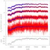 |
Fig. 1 Simulated spectra of a CSP at 13 Gyr from the onset of the SFH (exponentially delayed with τ = 0.3 Gyr), with solar metallicity and S/N 2, 5, 10, 20 and 30, increasing from bottom to top. For each S/N, the blue curve is the starting BC03 model used for the simulation, while the red curve is the simulated spectrum. The lower panel shows the behaviour of the S/N as a function of wavelength for a simulated spectra with S/N = 30 in the 6500–7000 Å window. |
To fit the input simulated spectra, we create a spectral library containing 176 BC03 simple stellar population (SSP) spectra. We choose four different metallicities for the synthetic spectra (Z = 0.004, Z = 0.008, Z = 0.02, Z = 0.05) and ages in the range 0.001 to 14 Gyr. In particular, to produce a well-sampled spectral library which would help to reconstruct the SFH of the input CSPs, we define a smaller time step (0.01 Gyr) for very young ages, to take into account the very different spectral shape of stellar populations younger than 1 Gyr; a larger (0.5 Gyr) time step is adopted for older SSPs. We fit the input spectra within the full range 3500−8500 Å and, as required by STARLIGHT, we fix the normalization wavelength for the spectral fitting at the line-free wavelength of 5520 Å, thus avoiding absorption features which could influence our results. We perform these fits in the two cases of masking or not the input spectral regions related to emission, or depending on α-element abundances (all the masked regions are reported in Table 1), which are not modelled by the BC03 synthetic spectra. Throughout the paper, we mainly discuss the results obtained in the second case, since it is more general and easily comparable with the literature.
Spectral regions masked in the fit.
2.1. Definition of the evolutionary properties
Since our tests on STARLIGHT are based on the comparison between input and output quantities, a consistent and accurate definition of them is necessary. In particular, we use mass-weighted properties, instead of light-weighted ones, since they allow near-independence of the choice of the normalization wavelength for the fit. Furthermore, mass-weighted quantities have the advantage of offering a more direct probe to the integrated SFH being not biased towards younger ages. Indeed, it is well-known that younger populations can dominate the luminosity of a stellar population, even when they contribute very little to the mass (Trager et al. 2000; Conroy 2013). Throughout this work, we also compare the retrieved mass-weighted and light-weighted properties (see Sect. 4).
-
Age. Following the definition given by Gallazzi et al. (2005) and Barber et al. (2007), we define the input ages as mass- and light-weighted ages, according to the following equations:
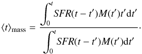
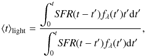 where M(t′) is the stellar mass provided by an SSP of age t′, fλ is the flux at a given wavelength2 of an SSP of age t′ and SFR(t−t′) is the star formation rate at the time (t−t′), when the SSP was formed. These equations account for the fact that a composite stellar population can be treated as the sum of many SSPs of different age. Thus each SSP, with a certain age t′, contributes to the global mass- (light-) weighted age of the CSP according to its mass (flux) and to the SFR at the time of its formation. For the output quantities, we define the retrieved output mass- and light- weighted ages by means of the mass- and light-fraction population vectors, according to the equations:
  (1)and
  (2)where agej is the age of the model component j, while mj and xj are its fractional contribution to the best fit model, respectively, provided by the STARLIGHT code.
 -
Age of formation. Starting from the output mass-weighted ages, we define the “age of formation” agef (i.e. look-back time) of the analyzed galaxies as:
 (3)where agemodel is the original age of each model in our spectral library and Δt = [ageU(z = 0)−ageU(z)] is the difference between the age of the Universe today and the age of the Universe at the redshift of the galaxy. In other words, agef allows us to consistently scale all the derived ages to z = 0.
 -
Metallicity. As said above, we consider solar metallicity (Z = 0.02) for the input simulated spectra; we define the output metallicities only as mass-weighted metallicities, employing the following equation:
 (4)where Zj is the metallicity of the model component j.
 -
Star formation histories. In general, considering that a CSP can be viewed as the sum of many SSPs (see Eq. (1) in Bruzual & Charlot 2003), the SFH of a stellar population can be understood as the fraction of stellar mass produced as a function of time in the form of SSPs. For this reason, the mass fractions mj provided by STARLIGHT plotted as function of the library SSPs ages can be considered as a direct proxy for the output SFH. Starting from this, we use the following equation to define the input SFH:
 where dt′ was introduced to make SFHin dimensionless, just like the output mj.
 -
Extinction and velocity dispersion. Extinction and velocity dispersion are direct STARLIGHT output, so we compare them directly with the chosen input ones (i.e. AV = 0 mag and σ = 200 km s-1).
2.2. Results from the simulations
2.2.1. Age and metallicity
The two top panels of Fig. 2 illustrate the results concerning ages and metallicities. In this figure we show the median differences, averaged on all the realized simulations at each S/N, between the output and the input quantites as a function of the mean S/N of the simulated spectra, together with their median absolute deviation (MAD)3, calculated at each S/N on the available simulations. We found that the differences and the relative dispersions effectively decrease with increasing S/N, as expected. In the case of the ages, only a small systematic shift of about +0.3 Gyr is present at S/N ≳ 10. To better quantify our results, we defined the percentage accuracy as the ratio between the dispersion of a given quantity on all the simulations at a given S/N and its true value, calculating the minimum S/N at which the input properties are retrieved with a percentage accuracy higher than ~10%.
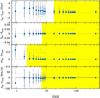 |
Fig. 2 Retrieved ages, metallicities, dust extinctions and velocity dispersions as a function of the mean S/N of the input spectra. Blue-filled circles represent the differences, averaged over all the computed simulations (i.e. 10×13 models), between the ouptut and the input mass-weighted ages, mass-weighted metallicities, dust extinctions and velocity dispersions (from top to bottom); blue vertical bars are the median absolute deviations (MAD) on all the computed simulations; grey points are the differences derived from each individual simulation; yellow shaded regions in each panel indicate the minimum S/N from which the accuracy of the input retrieving is better than 10%. |
We find minimum S/N values of ~18 for ages and ~9 for metallicities. Table 2 lists the median shifts and the median dispersions (together with their percentage values) which we find in the case of S/N = 100, which is close to the typical S/N of the median stacked spectra which we are will analyze in Sect. 3 (results for S/N = 20 are also shown to facilitate the comparison with literature).
We find that, masking the spectral regions associated with emission or depending on α-element abundances, the S/N needed to reach a percentage accuracy larger than the 10% increases to ~40 for mass-weighted ages, remaining unchanged for the other quantities. We ascribe this effect to the fact that we are exluding from the fit some spectral regions which are well-known age indicators (e.g. the Hβ line, see Burstein et al. 1984; Worthey et al. 1994).
2.2.2. Dust extinction and velocity dispersion
Dust extinction and velocity dispersion are retrieved with a percentage accuracy higher than the 10% for S/N ≳ 7 and ≳3, respectively, as illustrated in the two lowest panels of Fig. 2 and reported in Table 2. The results are in agreement with those obtained by Choi et al. (2014), who used another full-spectrum fitting code (developed by Conroy & van Dokkum 2012) and by Magris et al. (2015), who adopted the STARLIGHT code itself. Indeed, these authors found that age, metallicity, velocity dispersion and dust extinction are recovered without significant systematic offsets starting from S/N ≳ 10. In particular, for a S/N of 20, their median percentage shifts are ≲10% on age and metallicity (Choi et al. 2014) and ~8% on σ (Magris et al. 2015), while their dispersions are ≲10% on age and metallicity (Choi et al. 2014) and ~15% on σ (Magris et al. 2015). All these values are in agreement with ours at the same S/N (see Table 2).
Moreover, if we mask the spectral regions listed in Table 1, similar S/N of ~3 and ~8 are needed to recover dust extinction and velocity dispersion with a percentage accuracy better than 10%, respectively.
2.2.3. Star-formation histories including a single CSP
To quantify the accuracy with which the SFHs are retrieved, we calculate the percentage of mass gathered around the peak of the SFH, comparing the results with the theoretical expectations, as illustrated in Fig. 3. Here, the case of a S/N = 50 CSP input spectrum at four different ages from the onset of the SFH is shown. In particular, we find that the theoretical exponentially-delayed SFH assumed for the input spectra (rebinned at the age step of our SSP library models) is narrow, encompassing ~100% of mass within an age interval range of −1 Gyr to + 0.5 Gyr around its maximum. In comparison, for S/N ≳ 10, the retrieved SFHs appear slightly broader with respect to the theoretical one. Indeed, ~80% of mass is gathered within [−1; + 0.5] Gyr for CSPs younger than 5 Gyr, and an even larger age interval of [−1.5; + 1] Gyr is necessary to get this same mass percentage in the case of older populations. This dependence is illustrated in a more general way in Fig. 4 which shows the median mass fractions gathered around the SFH peak as a function of the mean S/N of the simulated spectra, for four CSPs. It is possible to note that CSPs older than 5 Gyr require larger age intervals around the SFH maximum to gather the same mass percentage as younger stellar populations. However, since a significant percentage of mass (70−80%) is always reached within ~1 Gyr from the peak of the SFH at any age, we conclude that the full-spectrum fitting succeeds in reproducing the input SFH for S/N ≳ 10. Finally, we find that STARLIGHT does not have any bias toward young ages, since, at any S/N, no mass is gathered at ages younger than 0.5 Gyr, except in the case of the youngest CSP (these results are valid also when the mask is applied to the input spectra). To summarize, from our tests we can conclude that the full-spectrum fitting with STARLIGHT is reliable if S/N ≳ 10–20 are considered. These S/Ns are lower or equal than those of typical SDSS individual spectra (i.e. ~20) and well below the typical S/N of stacked spectra, which are mainly used for high redshift studies (see Sect. 3.1).
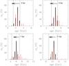 |
Fig. 3 Recovery of star formation histories. The four panels show a CSP at 3, 5, 7 and 11 Gyr from the onset of the SFH. Black vertical lines represent the exponentially delayed SFH (τ = 0.3 Gyr) assumed for the input spectra (rebinned according to the age step of our library models), while vertical lines represent the output SFH; horizontal arrows indicate the time from the beginning of the SF (i.e. 3, 5, 7 and 11 Gyr, respectively), while grey vertical lines mark the asymmetric age ranges around the SFH peak defined in the text for CSPs younger or older than 5 Gyr (i.e. [−1; + 0.5] and [−1.5; + 1], respectively). |
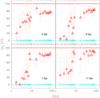 |
Fig. 4 Recovery of star formation histories. The four panels show a CSP at 3, 5, 7, and 11 Gyr from the onset of the SFH. In the two top panels, red triangles indicate the median mass fractions retrieved within [−1; + 0.5] Gyr from the SFH peak; in the two bottom panels, they are the median mass fractions within [−1.5; + 1] Gyr (as described in the text). In all four panels, cyan circles are the median mass fractions relative to stellar populations younger than 0.5 Gyr, while red and cyan horizontal lines mark the expected mass fraction within the defined age ranges and below 0.5 Gyr, respectively. |
Median shift and dispersion from the simulation of ETGs spectra, for S/N = 20 and 100 and BC03 spectral synthesis models.
2.2.4. More complex star-formation histories
Since the star-formation histories of galaxies (ETGs included, e.g. De Lucia et al. 2006; Maraston et al. 2009) can be stochastic and include multiple bursts, we also verify the full-spectrum fitting capabilities to retrieve more complex SFHs. In particular, we take an 11 Gyr old composite stellar population with an exponentially delayed SF (τ = 0.3 Gyr) as the main SF episode (this age is compatible with the age of the Universe at z ~ 0.15, which is the median redshift of our sample, see Sect. 3). We then define more complex SFHs by combining this single CSP with a burst of SF at different ages (5, 6, 7 Gyr) and with different mass contributions (3, 5, 10 %). In all cases, we consider a solar metallicity for the main SF episode and, according to the results of Maraston et al. (2009), a subsolar metallicity (Z = 0.004) for the later one. We do not mask any spectral feature of the input spectra, we assume AV = 0.1 mag for the two components and apply a velocity dispersion of 200 km s-1. We show the results for a S/N of 80, which matches the typical S/N of the SDSS median stacked spectra analyzed in the following (see Sect. 3). Useful information can be derived from the comparison between the output SFH obtained from these input simulated spectra and the one provided when the single CSP alone is taken as input SFH. Fig. 5 shows that the single CSP alone is well recovered by the full spectrum fitting. In particular, ~80% of the stellar mass is retrieved within ~1 Gyr from the SFH peak. When a burst is added to this major episode of SF, the full-spectrum fitting is able to recognize the presence of a more complex SFH, as indicated by the tail appearing at smaller ages, and the total mass percentage of the later burst is retrieved within 1 Gyr from the expected age. However, we note that the main episode of SF is spread on a time interval longer than expected, and 50% of the stellar mass is retrieved around ~1 Gyr from the SFR peak. We also find that, in this case, the mean properties of the global stellar population are well retrieved, with a percentage accuracy larger than 10% starting from S/N ~ 15 for age, ~7 for metallicity, ~20 for AV, ~8 for σ and that the metallicities of the two SF episodes are separately recovered. These S/Ns are well below those typical of the stacked spectra analyzed in the following sections.
In Fig. 6, we analyze the recovery of more complex SFHs as a function of the age and the mass contribution of the later SF burst. In particular, we find that the SFH tail, indicative of the presence of more recent SF episodes, arises for bursts happening ≳6 Gyr after the main SF event and contributing in mass by ≳5%. Therefore, under these conditions, it is possible for the full-spectrum fitting to recognize the SFH complexity. Furthermore, if mergers have played a role in the galaxy star-formation history, these tests suggest that our method would be sensitive to variations in SFR produced by mergers among galaxies of different ages, but it is intrinsically unable to discern whether or not mergers among galaxies of similar age (coeval mergers), which increase stellar masses and sizes leaving the shape of the SFH unchanged, occurred during the galaxy evolution to build galaxy mass.
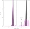 |
Fig. 5 Retrieving of more complex SFH. Left panel: output SFH (pink curve) obtained when an input SFH (grey curve) including only a single CSP is considered; right panel: output SFH (pink curve) obtained when an input SFH (grey curve and vertical line) including a single CSP plus a later burst (which happens 6 Gyr after the main SF episode and contributing 5% to the total mass. |
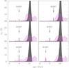 |
Fig. 6 Retrieving of more complex SFHs as a function of the age and the mass contribution of the later burst. Left panels show the output SFH (pink curves) obtained when the input SFH (grey curves and vertical lines) includes a single CSP plus a later burst happening 6 Gyr after the main SF episode and contributing in mass by 3, 5 and 10% (from top to bottom). Right panels show the output SFH (pink curves) obtained when the input SFH (grey curves and vertical lines) includes a single CSP plus a later burst of SF contributing 5% to the total mass, and happening 4, 6, or 8 Gyr after the main SF event (from top to bottom). |
2.3. Testing different stellar population synthesis models
Having adopted BC03 models to set up both the input simulated spectra and the spectral library, in this section we verify if this choice can affect the results. This is a simple consistency check to verify the full-spectrum fitting capabilities for retrieving the galaxy evolutionary properties starting from the same input spectra. With this aim, using the procedure described in Sect. 2 we simulate, 13 simple stellar population (SSP) spectra with solar metallicities and ages from 1 to 13 Gyr in steps of 1 Gyr, starting from BC03 spectra, within the same S/N range defined in Sect. 2. We fit them with the spectral library of Maraston & Strömbäck (2011; MS11) SSP models which are defined in the wavelength range 3200−9300 Å, are based on the STELIB stellar spectra library (Le Borgne et al. 2003), have a resolution of 3 Å, and assume a Kroupa IMF (Kroupa 2001). We show in Fig. 7 the recovery of age, metallicity, velocity dispersion and dust extinction, in analogy with Fig. 2. Also in this case, the percentage accuracy of 10% is reached at similar S/N, which are ~5 for age, ~7 for velocity dispersion and ~3 for dust extinction, while metallicity is retrieved with basically no bias at every S/N. However, as it is possible to note, a difference between the retrieved mass-weighted ages and the true ages is also present at high S/N. This overestimation can be explained by the fact that, due to a different treatment of the TP-AGB phase and of the convective overshooting in the stellar interiors, MS11 models are on average more blue than BC03 ones (see Maraston et al. 2006 for further details). This implies that, for the same metallicity, older MS11 models are chosen to best-fit BC03 input spectra, to compensate the bluer colours.
To avoid biases against MS11 models, we also fit an ensemble of 13 MS11 simulated spectra with a spectral library made up of MS11 models themselves (this test is performed using MILES – see Sánchez-Blázquez et al. 2006 – stellar spectra both for the input and the library synthetic models). For computational feasibility, we create in this case a less extended grid of S/N for the input simulated spectra and, to be consistent with the results shown for BC03 models, we do not adopt the mask for the input spectra. In this case, we find that the evolutionary properties are retrieved with a percentage accuracy larger than the 10% starting from a S/N of ~25 for mass-weighted ages, ~15 for metallicities, ~30 for dust extinction and ~6 for velocity dispersion. These values are in general higher than those found using BC03 models, but it is important to note that they are below those of the median stacked spectra analyzed in the following sections (see Sect. 3).
3. Sample selection
We analyze a sample of 24 488 very massive and passive early-type galaxies with 0.02 ≲ z ≲ 0.3. The restriction to the most passive ETGs is indeed very useful to investigate galaxy evolution, since it allows us to address the galaxy mass assembly history in the very early epochs.
The adopted sample was already used by Moresco et al. (2011, M11; see this work for more details), who matched SDSS-DR6 galaxies with the Two Micron All Sky Survey (2MASS; with photometry in the J, H and K bands) to achieve a larger wavelength coverage, thus obtaining better estimates of stellar masses from SED-fitting and photometric data. According to the criteria explained in M11, the analyzed galaxies have no strong emission lines (rest-frame equivalent width EW(Hα) > −5 Å and EW ([OII]λ3727) > −5 Å) and spectral energy distribution matching the reddest passive ETG templates, according to the Ilbert et al. (2006) criteria. Finally, the sample was cross-matched with the SDSS DR4 subsample obtained by Gallazzi et al. (2005), for which stellar metallicity estimates have been performed by means of a set of Lick absorption indices (see Sect. 4.5). Moreover, to deal only with the most massive galaxies, only objects with log (M/M⊙) > 10.75 were included in the sample (above this threshold, the galaxy number density is found to be almost constant up to z ~ 1, see Pozzetti et al. 2010) which, in addition, was split into four narrow mass bins (Δlog (M/M⊙ = 0.25): 10.75 < log (M/M⊙) < 11, 11 < log (M/M⊙) < 11.25, 11.25 < log (M/M⊙) < 11.5, and log (M/M⊙) > 11.5 (Table 3 reports the number of objects contained in each mass bin), in turn divided into various redshift bins of width Δz ~ 0.02. It is worth noting that, on average, the difference in median mass along the redshift range is negligible within the four mass slices our sample is divided into, showing no significant evolution as a function of redshift (Moresco et al. 2011, Concas et al., in prep.).
We also assess the morphology of the galaxies in our sample using the Sérsic index ρn (Sersic 1968), which correlates with the morphology because objects with n< 2.5 are disk-like (Andredakis et al. 1995), while those with n> 2.5 are bulge-dominated or spheroid (Ravindranath et al. 2004). In particular, the values of ρn are taken from the NYU Value-Added Galaxy catalogue (Blanton et al. 2005), which contains photometric and spectroscopic information on a sample of ~2.5 × 10⁷ galaxies extracted from the SDSS DR7. From this check, we derive that ~96% of the analyzed galaxies are bulge-dominated systems.
3.1. Median stacked spectra
In order to increase the S/N of the input spectra, we work on the median stacked spectra derived for each mass and redshift bin. A stacked spectrum is produced by shifting each individual rest-frame spectrum, normalized to a chosen wavelength, to the rest frame and then by constructing, via interpolation, a grid of common wavelengths at which the median (or mean) flux is computed. In our sample, the median stacked spectra were obtained for each mass and redshift bin (see Sect. 3). We define the error on the median stacked flux as MAD/ , were MAD is the median absolute deviation and N is the number of objects at each wavelength. Before stacking them together, we normalized each individual spectrum at rest-frame 5000 Å, where no strong absorption features are present which could influence the final result. The error on the final stacked spectrum was corrected in order to obtain more reliable values for the χ2 distribution provided by the spectral fit. In particular, we readjusted the original error eλ of the spectra making it comparable with the data dispersion of (Oλ−Mλ) (where Oλ are the observed data, Mλ is the best fit model obtained from the first-round fit). After the error redefinition, the signal-to-noise ratios of the median stacked spectra are ~80 (the error eλ is, on average, increased by a factor of ~7).
The main characteristics of the analyzed median stacked spectra are illustrated in Fig. 8, where also the fractional differences among the various spectra are shown to better visualize their differences as a function of wavelength. We note that median stacked spectra are completely emission lines-free. Moreover, two clear observational trends are present, with spectra getting redder both with cosmic time and increasing mass. In the following, our aim is to investigate these observed trends by means of the full-spectrum fitting technique. In Sect. 5, we also verify that the use of stacked spectra does not introduce biases into the results, concluding that they can be employed at high redshift to increase the S/N of the observed spectra.
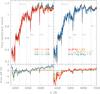 |
Fig. 8 SDSS median stacked spectra for the sample of massive and passive ETGs. Left and right upper panels show, respectively, median stacked spectra with a fixed redshift (0.15 ≲ z ≲ 0.19) and different masses (with mass increasing from blue to red) and with a fixed mass (11.25 < log (M/M⊙) < 11.5) and four different redshifts (0.04, 0.08, 0.16, 0.23) (with redshift increasing from blue to red). Lower panels illustrate the fractional differences (defined as (fi−fREF/fREF) × 100, where fi is the flux of the ith spectrum and fREF is the reference flux) among the stacked spectra as a function of wavelength. In particular, to show the redshift and the mass dependence we used as reference, respectively, the median stacked spectrum obtained for 11.25 < log (M/M⊙) < 11.5 and 0.07 < z < 0.09, and the one corresponding to 10.75 < log (M/M⊙) < 11 and 0.15 < z < 0.17. Vertical grey lines mark some of the best-known absorption lines. |
4. Evolutionary properties from the full-spectrum fitting of median stacked spectra
To infer the evolutionary and physical properties of our sample, we fit the median stacked spectra for each mass and redshift bin, mainly using BC03 spectra, but also exploiting a spectral library of MS11 STELIB models. In all cases, we fix the wavelength range for the spectral fitting to 3500−7000 Å for all the mass and redshift bins, in order to avoid redshift-dependent results.Both the BC03 and the MS11 spectral libraries contain spectra with ages starting from 0.01 Gyr and not exceeding the age of the Universe at the redshift of the stacked spectrum itself.
We use the metallicities Z = 0.004,0.008,0.02,0.05 for the BC03 library and Z = 0.01,0.02,0.04 for that of MS11 and we assume a Calzetti attenuation curve to account for the presence of dust (Calzetti 2001). Moreover, contrary to our method in Sect. 2, in both cases we mask the spectral regions of the input spectra which are associated with emission lines (Cid Fernandes et al. 2005) and α-element dependent lines (Thomas et al. 2003), since they are not modelled by BC03 and MS11 synthetic spectra (see Table 1 and grey shaded regions in Fig. 9).
As we can see from Fig. 9, the best fit model produced by the spectral fitting matches correctly the input spectrum, both in the case of BC03 and MS11 models. The dispersion on the mean ratio between the synthetic and observed flux on all the not-masked pixels is ≲2%.
From the comparison between the observed and the synthetic spectra, signs of a residual emission in correspondence of the masked spectral regions can be noticed. We discuss this residual emission in a parallel paper, which is dedicated to the study of the Hβ absorption line (Concas et al., in prep.).
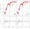 |
Fig. 9 Typical output of the full-spectrum fitting procedure using BC03 (left) and MS11 (right) spectral synthesis models. In particular, we show the case of the median stacked spectrum derived for 11 < log (M/M⊙) < 11.25 and z ~ 0.05. In the top panel the black curve is the observed spectrum, the red curve is the best fit model and grey shaded regions are the masked spectral regions (see Table 1). The bottom panel shows the ratio of the best fit model spectrum to the observed flux. |
4.1. Error estimates
Throughout the data analysis, the uncertainties on the investigated evolutionary and physical properties are derived in three different ways, defined as follows:
-
rmssim: this is the dispersion derived in Sect. 2.2 at the typical S/N of the analyzed median stacked spectra (i.e. S/N ~ 100);
-
err100: this error is derived by comparing the results obtained from computing 100 realizations of each median stacked spectrum within its error (defined in Sect. 3.1);
-
rmsset: this dispersion is calculated by comparing the results obtained by changing some setting parameters of the spectral fit (e.g. the number of the masked spectral regions, the upper limit for dust extinction, and the extension of the library in age or metallicity).
4.2. Ages
Using Eq. (1), we derive the mass-weighted ages of our galaxies, illustrated in the upper panel of Fig. 10. Considering the observed properties of the median stacked spectra with mass and redshift illustrated in Fig. 8, we find an evolutionary trend, with mass-weighted ages increasing systematically with mass (for a fixed redshift), as well as with cosmic time (for a given mass bin). In particular, ages vary from ~10 to ~13 Gyr, increasing by ~0.4 Gyr from the lowest to the highest masses, in agreement with the observational trends shown in Fig. 8. The lower panel of Fig. 10 illustrates, instead, the retrieved light-weighted ages, which increase by ~1 Gyr from the lowest to the highest mass. Light-weighted ages are younger than mass-weighted ones, with a difference of ~0.6 Gyr in the lowest redshift bins and of ~1 Gyr in the highest ones, on average (Table 4 lists the three uncertainties estimates rmssim, err100 and rmsset derived for ⟨ t ⟩ mass).
It is interesting to note that, even when the cosmological constraint is relaxed and the maximum allowed age for the spectral library models is pushed to 14 Gyr at all redshifts, the trend of the mass-weighted age with both mass and cosmic time still holds, and only in few cases the mass-weighted ages exceed the age of the Universe. Figure 11 illustrates our mass-weighted ages as a function of the velocity dispersion (see Sect. 4.6). At z< 0.1, we find that they are compatible, within the dispersion (~25%), with the relation derived by McDermid et al. (2015) from the analysis of the ATLAS3D sample (z ≲ 0.1 and 9.5 < log (Mdyn/M⊙) < 12) by means of the PPXF code (Cappellari & Emsellem 2004). At z ≲ 0.06, for a given velocity dispersion, our mass-weighted ages are instead older than those deduced by Thomas et al. (2010). This can be due to the fact that, unlike our approach, they analyzed a sample of ~3600 morphologically selected galaxies (i.e. MOSES ETGs at 0.05 ≤ z ≤ 0.06, see Schawinski et al. 2007), without restricting thir method to the most passive objects and also to the fact that, using the Lick indices, they derive SSP-equivalent instead of mass-weighted ages.
It is also interesting to note that our average light-weighted ages for z ≲ 0.06 are ~11.6 Gyr for all of the four mass bins and that these values are in agreement with those obtained at similar redshifts by Conroy et al. (2014), who applied the stellar population synthesis (SPS) model developed by Conroy & van Dokkum (2012) to a sample of nearby (0.025 <z< 0.06) SDSS DR7 ETGs, with masses comparable to ours (i.e. 10.70 < log (M/M⊙) < 11.07).
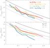 |
Fig. 10 Mass-weighted (top) and light-weighted (bottom) age-redshift relations (for BC03 models). Stellar mass increases from blue to red. The black line is the age of the Universe, while grey lines are the age of galaxies assuming different formation redshifts. |
The derived mass-weighted ages imply a very early epoch of formation. A further confirmation of this comes from Fig. 12, which illustrates the ETGs mass-weighted ages of formation (see Eq. (3)) as a function of mass and redshift (in this case, the term ageU(z) in Eq. (3) is the age of the Universe at the redshift of each of the available median stacked spectra), together with the 1σ dispersions calculated from the 16th and 84th percentiles of the mass fraction cumulative distribution. As it is possible to note, the mass-weighted ages of formation are very high, with an increase of ~0.4 Gyr from low to high masses. Taking into account the 1σ dispersion on the SFHs, we also find that the slopes of the agef−z relations are compatible with zero, indicating that, at a fixed mass, the analyzed galaxies have similar zF, especially in the highest mass bins. However, it is important to note that our main results concerning SFHs do not rely on the fact that galaxies in the same mass bin have similar formation epochs, since the spectral fits are realized separately on each mass and redshift bin.
Using MS11 models, we find the same trends of the mass-weighted agef with mass and redshift. In particular, in this case agef are only ~0.2 Gyr older than the ones provided by BC03 spectra, on average. In both cases, the independence of agef of redshift is also an indication that we are not biased towards young galaxy progenitors going to higher redshift, and thus that our sample is not affected by the so-called progenitor bias (van Dokkum & Franx 1996).
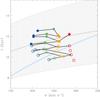 |
Fig. 11 Mass-weighted ages as a function of the velocity dispersion σ for BC03 models (symbols are colour-coded as in Fig. 10). Filled circles are the mass-weighted ages corresponding to z< 0.1, matching the redshifts analyzed by McDermid et al. (2015), with black curves linking the mass-weighted ages related to different mass bins but similar redshifts. The grey curve is the age – σ relation inferred by McDermid et al. (2015) with its dispersion (grey shaded region), while the light-blue curve is the Thomas et al. (2010) relation (its dispersion, not shown in the figure, is in the order of 60%). |
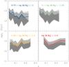 |
Fig. 12 agef-redshift relations for the four mass bins. Solid and dotted curves (colour coded as in Fig. 10) are the ages of formation as a function of redshift referring, respectively to BC03 and MS11 spectral synthesis models. Dark-grey and light-grey shaded regions are the 1σ dispersions calculated starting from the 16th (P16) and 84th (P84) percentiles of the mass fraction cumulative function for BC03 and MS11 models, respectively. |
4.3. Star-formation histories
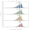 |
Fig. 13 Mass fractions mj as a function of look-back time for the four mass bins, with mass increasing from top to bottom (in the case of BC03 models). Colored vertical lines (colour-coded as in Fig. 10) are the mj obtained from the full-spectrum fitting for each mass bin, put in phase according to their P50. In each mass bin, black vertical lines mark the P50 of the distribution, obtained from data as an average of the P50 of all the redshift bins, while black horizontal lines are the median dispersions [P50 – P16] and [P84 – P50]. The corresponding asymmetric Gaussians (grey) are overplotted on the mj distributions. On the top of the figure, the zF corresponding to each agef is indicated. |
In this section we investigate the mass trend of the SFHs by looking at the mass fractions provided by the full-spectrum fitting (mj) as a function of the mass-weighted age of formation, agef. In particular, we consider all the redshifts of a given mass bin together, in order to visualize the shape of the SFH as a function of mass. The behaviour of the mj distribution is illustrated in Fig. 13, where asymmetric Gaussians - constructed starting from the 50th (P50), 16th (P16) and 84th (P84) percentiles of the mass fraction distribution cumulative functions – are overplotted on the mj to better visualize the distribution (P16 and P84 allow us to compute the dispersion of the distribution within 1σ). For a given mass bin, P50 is the median on the P50 of all the available redshifts, while the asymmetric dispersions are defined as the median differences [P84 – P50] and [P50 – P16], averaged in the same way. Table 3 lists the calculated values for the four mass bins. To best retrieve the shape of the SFHs and minimize the dependence on possible small differences in zF, we decide to put the mj distributions in phase, by synchronizing the P50 of each redshift bin to the median P50 of each mass bin, in order not to rely on the assumption that galaxies in a given mass bin have the same formation epochs.
From the figure it is possible to note that the median of the asymmetric Gaussians slightly increases with mass and that the width of the Gaussians decreases from low to high mass. In particular, we find that the width [P84 – P16] decreases from ~1 Gyr to ~0.7 Gyr from low to high masses, while P50 increases by ~0.2 Gyr. MS11 models produce slightly higher P50, which increase by ~0.1 Gyr with mass, and dispersions [P84 – P16] of ~0.35 Gyr, regardless of mass.
Considering these results and our largest uncertainty on age rmsset (see Table 4), the derived trends show that massive galaxies have already formed ~50% of the stellar mass by z ≳ 5 (z ≳ 3 if the ~0.5 Gyr systematic is taken into account, see Sect. 5). In addition, this percentage of mass is formed slightly earlier in more massive galaxies than in less massive ones, with the former also having shorter star formation histories than the latter (see Fig. 13 and Table 3).
We quantify the typical SFR of the analyzed galaxies defining, for each mass bin, the quantity  (5)based on the assumption that the 68% of the stellar mass is formed whithin 68% time interval Δt around the peak of the SFH. We find that the typical SFRs increase for increasing mass from ~50 to ~370 M⊙ yr-1 (SFR ~ 140−750 M⊙yr-1 for MS11 models).
The evolutionary picture emerging from the analysis of the star-formation histories can be also deduced from Fig. 14, which illustrates the mass fraction relative to the stellar populations older or younger than 5 Gyr. Regardless of redshift and mass, we derive that ≲6% of the stellar mass in our galaxies comes from stellar populations younger than 5 Gyr (≲20% when we consider light fractions instead of mass fractions) and that this fraction decreases to ≲4% and ≲1% if we consider a threshold of 1 and 0.5 Gyr, respectively. Moreover, the old and the young mass fractions are specular to each other, with the young one decreasing with both mass and cosmic time, contrary to the old one: this suggests that more massive galaxies assembled a higher fraction of their mass earlier than less massive systems. The fact that the analyzed galaxies have not experienced significant bursts of star formation in recent times is also shown in Fig. 15 (these bursts would be recognized by the full-spectrum fitting, as discussed in Sect. 2.2). MS11 spectral synthesis models confirm these trends, providing a similar low percentage of stellar mass below 5 Gyr (i.e. <7%) and an even smaller contribution (<0.1%) of the stellar populations younger than 1 Gyr to the total mass (which also implies slightly older mass-weighted ages).
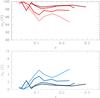 |
Fig. 14 Mass fractions mj recovered from the full-spectrum fitting as a function of redshift in the case of BC03 models. Red and blue curves refer, respectively, to stellar populations older and younger than 5 Gyr, with darker colours standing for higher stellar masses. |
Number of galaxies, statistical, evolutionary and physical properties of the four mass bins of our sample (in the case of BC03 models).
Uncertainties on ages, metallicities, velocity dispersions and dust extinction provided by the three different estimates described in the text (in the case of BC03 models).
4.4. The shape of the star-formation history
The SFH of individual galaxies has been often approximated by simple declining exponential functions SFR(t) ∝ exp(−t/τ), where t is the galaxy age and τ is the star formation timescale (Expdel hereafter). Despite the success of these models for estimating the stellar masses of nearby spiral galaxies (Bell & de Jong 2001), recently many results have begun to highlight their limitations, especially when applied to higher redshift samples (Papovich et al. 2001; Shapley et al. 2005; Stark et al. 2009). Since then, other functional forms have been considered: for example, delayed-τ (exponentially delayed) models (with τ being the SF timescale), in which SFR(t) ∝ τ-2t exp(−t/τ) (Bruzual & Kron 1980; Bruzual & Charlot 2003; Moustakas et al. 2013; Pacifici et al. 2013) or “inverted-τ” models of the form SFR(t) ∝ exp( + t/τ) (Maraston et al. 2010; Pforr et al. 2012) have been suggested to be a better way to represent the SFH of massive galaxies at intermediate or high redshift.
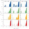 |
Fig. 15 SFHs derived from median stacked spectra. Mass increases from top to bottom, redshift increases from left to right, as indicated. Note that no significant episodes of SF occurred after the main SF event. The mass fractions relative to stellar population younger than 5 Gyr is very low (i.e. ≲5%). |
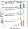 |
Fig. 16 SFH for the four mass bins of our sample, with mass increasing from top to bottom (in the case of BC03 models). Colored vertical lines are the SFR (M⊙ yr-1) derived from the mj provided by the spectral fitting (colours are coded as in Fig. 10). In each mass bin, black vertical and horizontal lines are defined as in Fig. 13. In each panel, we show the two best fit models deriving from the assumption of an Expdel (dotted curves) or an Expdelc (solid curves) parametric function to describe the derived SFHs. The best fit parameters are also reported. Pink curves are the inverted-τ models with τ = 0.3 Gyr described in the text, extended up to 13.48 Gyr (which corresponds to the age of the Universe in the assumed cosmology). |
In this section, we test if these two analytical forms are able to describe the SFH of massive and passive, low redshift ETGs. We also introduce the parametric function (Expdelc hereafter): 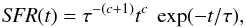 (6)with c being a real number ranging from 0 to 1 with steps of 0.01, which parametrizes how fast the SFR rises at early ages.
The results are shown in Fig. 16, in which we illustrate the SFR derived from the mass fractions mj as a function of the look-back time (age of formation), together with the delayed-τ and the inverted-τ models.
For each mass and redshift bin, the observed SFRs are derived using the following equation: 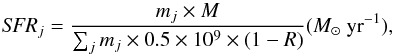 (7)where mj are the mass fractions obtained from the full-spectrum fitting, ∑ jmj is the sum of the mass fractions of each mass and redshift bin, M is the total stellar mass, the term 0.5 × 10⁹yr is the time step of our spectral library and R is the “return fraction”, which represents the fraction of mass which is returned to the ISM by supernovae-driven winds and mass losses. In particular, considering both the mass weighted ages of our galaxies (i.e. ~10–13 Gyr) and the Chabrier IMF assumed in this work, we fix the value of R to 0.5 (see Bruzual & Charlot 2003).
To perform the data-to-model comparison in the case of exponentially delayed SFHs, we define a grid of models Expdel(τ) with different SF timescales τ (0.2 Gyr to 0.7 Gyr in steps of 0.01 Gyr). Then, by minimizing the quadratic differences ![Mathematical equation: \begin{equation} \sum_{j}{{[Expdel(\tau, {age_{\rm f}}_{j})-\textit{SFR}_{j}]}^{2}}, \end{equation}](/articles/aa/full_html/2016/08/aa27772-15/aa27772-15-eq219.png) (8)and
(8)and ![Mathematical equation: \begin{equation} \sum_{j}{{[Expdelc(\tau, c, {age_{\rm f}}_{j})-\textit{SFR}_{j}]}^{2}}, \end{equation}](/articles/aa/full_html/2016/08/aa27772-15/aa27772-15-eq220.png) (9)we find the τ and c which best reproduce the observed SFH in each mass and redshift bin, by fixing the P50 of data and models. Then, as in Sect. 4.3 for the mj distribution, we put the results obtained for all the redshifts in a given mass bin together, also putting their P50 in phase according to the median P50. The median values of τ and c on all the redshifts are thus taken as the best fit parameters for that given mass bin (see Fig. 16). We find that the standard delayed-τ models with shorter τ’s are needed to reproduce the observations for increasing mass. In particular, a value τ = 0.44 (with a dispersion of ±0.02 Gyr) is compatible with the SFH of less massive galaxies (10.75 < log (M/M⊙) < 11.25), while slightly shorter values (i.e. τ = 0.37, with a dispersion of ±0.02 Gyr) should be adopted to match the SFH at higher masses (log (M/M⊙) > 11.5). The Expdelc parametric form provides a much better fit to the data, with quadratic differences which are smaller even by two orders of magnitude than in the case of the Expdel form. Furthermore, slightly higher values of τ are found as best fit, decreasing for increasing mass from 0.8 Gyr (with a dispersion of ±0.1 Gyr) to 0.6 Gyr (with a dispersion of ±0.1 Gyr), while the best fit c is ~0.1 (with a dispersion of ±0.05) regardless of mass, and reproduces the very fast rise of the SFR (see Table 3). The derived values are compatible with the SF timescale Δt ~ 0.4 Gyr derived by Thomas et al. (2010) from the measure of the α-element abundance4. However, it must be mentioned that also using the [α/ Fe] ratios, Conroy et al. (2014) obtained longer SF timescale (Δt ~ 0.8 Gyr) for similar masses. In addition, it is worth noting that as shown in Sect. 2, the full-spectrum fitting tends to broaden the SFH for old stellar populations in the case of BC03 models (see Fig. 1) and thus the derived SF timescales could be effectively overestimated.
(9)we find the τ and c which best reproduce the observed SFH in each mass and redshift bin, by fixing the P50 of data and models. Then, as in Sect. 4.3 for the mj distribution, we put the results obtained for all the redshifts in a given mass bin together, also putting their P50 in phase according to the median P50. The median values of τ and c on all the redshifts are thus taken as the best fit parameters for that given mass bin (see Fig. 16). We find that the standard delayed-τ models with shorter τ’s are needed to reproduce the observations for increasing mass. In particular, a value τ = 0.44 (with a dispersion of ±0.02 Gyr) is compatible with the SFH of less massive galaxies (10.75 < log (M/M⊙) < 11.25), while slightly shorter values (i.e. τ = 0.37, with a dispersion of ±0.02 Gyr) should be adopted to match the SFH at higher masses (log (M/M⊙) > 11.5). The Expdelc parametric form provides a much better fit to the data, with quadratic differences which are smaller even by two orders of magnitude than in the case of the Expdel form. Furthermore, slightly higher values of τ are found as best fit, decreasing for increasing mass from 0.8 Gyr (with a dispersion of ±0.1 Gyr) to 0.6 Gyr (with a dispersion of ±0.1 Gyr), while the best fit c is ~0.1 (with a dispersion of ±0.05) regardless of mass, and reproduces the very fast rise of the SFR (see Table 3). The derived values are compatible with the SF timescale Δt ~ 0.4 Gyr derived by Thomas et al. (2010) from the measure of the α-element abundance4. However, it must be mentioned that also using the [α/ Fe] ratios, Conroy et al. (2014) obtained longer SF timescale (Δt ~ 0.8 Gyr) for similar masses. In addition, it is worth noting that as shown in Sect. 2, the full-spectrum fitting tends to broaden the SFH for old stellar populations in the case of BC03 models (see Fig. 1) and thus the derived SF timescales could be effectively overestimated.
However, in agreement with the BC03 analysis, also the best fits with MS11 models confirm the short e-folding times, which are τ ~ 0.25 Gyr (with a dispersion of ±0.0016 Gyr), regardless of mass (τ ~ 0.39 Gyr – with a dispersion of ±0.03 – and c ~ 0.1 – with a dispersion of ±0.02 – in the case of Expdelc, regardless of mass).
Figure 16 also illustrates “inverted-τ” models with τ = 0.3 Gyr, normalized at the SFR maximum in each mass bin. The increased difficulty in matching these models with the observations may be linked to our poor sampling of the SFH at very early ages.
Figure 16 confirms that the SFHs derived from our analysis are smooth and concentrated at high redshift. However, we are not able to distinguish whether these smooth SFHs are the result of a rapid collapse at high redshift or derive from coeval mergers. An important consideration is that the smoothness of the derived SFHs could be due to the fact that they derive from median stacked spectra, which represent the average behaviour of the sample. Therefore, the stochastic SF episodes related to the individual galaxies involved in the stack can be washed out and diluted within the stack. Our results must be taken with a statistical meaning because they are based on the analysis of stacked spectra. High S/N spectra of individual ETGs are required to better assess their evolution and star formation histories.
4.5. Metallicities
From the fit to the median stacked spectra, we also analyze the trends with mass and redshift of the retrieved mass-weighted metallicities ⟨ Z ⟩ mass, derived from Eq. (4). On average, we find supersolar metallicities, with ⟨ Z ⟩ mass ~ 0.029 ± 0.0015, as illustrated in Fig. 17 (a median value ⟨ Z ⟩ light ~ 0.025 is obtained in case of light-weighted metallicities). Our ⟨ Z ⟩ mass have no clear trend with redshift in a given mass bin, and also do not show a significant dependence on mass (metallicities increase on average by only 0.0025 from the lowest to the highest masses). The independence of metallicities of cosmic time is a suggestion that the analyzed galaxies are very old systems, which have depleted all their cold gas reservoir, with no further enrichment of their interstellar medium with new metals (however, we remind readers that the analyzed interval of cosmic time is not much extended, amounting to ~3.3 Gyr). The dependence on mass suggests that more massive galaxies are able to retain more metals thanks to their deeper potential wells (Tremonti et al. 2004).
We find that MS11 models also provide slightly supersolar metallicities (⟨ Z ⟩ mass ~ 0.027 ± 0.0020, on average), with a more remarkable dependence on mass (metallicity increases by ~0.005 from the lowest to the highest mass). The three uncertainty estimates rmssim, err100 and rmsset calculated on the mass-weighted metallicities are reported in Table 4.
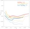 |
Fig. 17 Mass weighted metallicities as a function of mass and redshift. Solid and dotted curves refer to BC03 and MS11 models, respectively. Stellar mass increases from blue to red, as indicated in the top right of the figure. |
In Fig. 18, instead, we show a comparison between our metallicity estimates and the ones reported in the literature. In particular, we illustrate the scaling relation provided by Thomas et al. (2010) obtained from their sample of nearby ETGs5, with its observed average scatter. We also show the median metallicities measured on our sample by Gallazzi et al. (2005), together with their MADs. These metallicities are, in both cases, measured by fitting individual spectral features (Lick indices, Burstein et al. 1984). In particular, Thomas et al. (2010) derived their values from the measure of 24 Lick indices, while Gallazzi et al. (2005) used a set of five specific Lick indices, including Hβ, HδA, HγA, [Mg2Fe] and [MgFe] ′6.
We note that the metallicity estimates are broadly consistent, with a difference Δ ⟨ Z ⟩ (This work−Gallazzi) ~ + 0.0036 and Δ ⟨ Z ⟩ (This work−Thomas) ~ −0.0032. The figure also illustrates the McDermid et al. (2015) mass-weighted metallicity – velocity dispersion relation, which they derive by means of another full-spectrum fitting code (i.e. PPXF), using the Vazdekis synthetic models (Vazdekis et al. 2012). We find that their metallicities are closer to the solar value (i.e. Z ~ 0.02), with ⟨ ΔZ ⟩ (This work−McDermid) ~ − 0.01.
We ascribe the discrepancies among these various results mainly to the use of different sets of Lick indices or synthetic models (in the case of full-spectrum fitting). Therefore, even if there is agreement among the majority of the reported results in predicting supersolar metallicities (i.e. Z ≳ 0.025), which also increase with σ, it is evident that the absolute values of metallicities depend on the method and the assumptions used for their estimate.
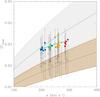 |
Fig. 18 Comparison between our mass-weighted metallicities (in the case of BC03 models) and the values reported in the literature. In particular, coloured filled circles (colour-coded as in Fig. 10) are our results (the cyan curve is a second order fit to our data); the grey curve is the scaling relation provided by Thomas et al. (2010), with its dispersion (grey shaded region), while black open circles and vertical bars are the measures (and dispersions) performed on our sample by Gallazzi et al. (2005). The light-brown curve is the relation derived by McDermid et al. (2015), together with its dispersion (light-brown shaded region). |
4.6. Velocity dispersions and dust extinction
In Fig. 19 we illustrate the trend of the velocity dispersion with stellar mass. In particular, we show the values obtained for all the redshift bins available for a given mass. We find velocity dispersions σ ~ 200−300 km s-1, increasing for increasing stellar mass. Our results are compared with the median values derived on the same sample by the Princeton group7, who have provided a re-reduction of a subsample of SDSS data. It is possible to note that there is a good agreement between the two estimates. Indeed, the differences Δσ(This Work−Princeton) are ≲12%. Furthermore, the largest discrepancies occur only in correspondence of the extreme low or high redshift bins, which have fewer statistics (i.e. which contain fewer objects), and that MS11 models provide velocity dispersions which are in agreement with the BC03 ones, being only ~3.5 km s-1 lower than them, on average.
As it is possible to note in Fig. 20, the visual extinction AV obtained from the spectral fit with BC03 models is always <0.2 mag and on average ~0.08 (averaging on the four mass bins), in agreement with the typical view of early-type galaxies being old and dust-free objects (Wise & Silva 1996; Saglia et al. 2000; Tojeiro et al. 2013). MS11 models also produce very low AV (<0.25 mag) which are, however, on average ~0.08 mag higher than the BC03 ones. Moreover, in the BC03 case, more massive galaxies have lower AV with respect to less massive ones, while this trend is much less remarkable when MS11 models are used. Although further investigations are needed to confirm the reliability of this trend, it may suggest that more massive galaxies are able to clear their interstellar medium more efficiently, probably due to more intense feedback processes linked with star formation or AGN activity. As usual, the value of rmssim, err100 and rmsset for both the velocity dispersions and dust extinction are reported in Table 4.
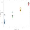 |
Fig. 19 Velocity dispersions σ as a function of mass (for BC03 models). Colored triangles represent our observed values at different redshifts for each mass bin (the values of σ are illustrated together with the errors MAD/ |
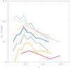 |
Fig. 20 Dust extinction AV as a function of redshift and mass. Solid and dotted curves refer to BC03 and MS11 models, respectively. Colors are coded as in Fig. 10. |
5. Testing the fitting of individual spectra
Since median stacked spectra are very useful to increase the S/N of the observed spectra, in this section we verify if the results obtained using median stacked spectra are consistent with those derived by fitting individual spectra (we performed this check in the case of BC03 models). In particular, we compare the ⟨ t ⟩ mass, ⟨ Z ⟩ mass, AV and σ derived so far through the median stacked spectra, with the median of their distributions obtained studying individual objects. We restrict our analysis to the two most massive bins (i.e. <11.25 < log (M/M⊙) < 11.5 and log (M/M⊙) > 11.5), both because they are the most interesting ones to investigate galaxy formation and evolution and for computational feasibility (since they contain fewer objects, see Table 3).
Figure 21 illustrates what is derived for ⟨ t ⟩ mass, ⟨ Z ⟩ mass, σ and AV at <11.25 < log (M/M⊙) < 11.5 and log (M/M⊙) > 11.5.
In most of the cases the results of median stacked spectra overlapped, within the dispersion, with those of individual spectra. We found that ages, metallicities and velocity dispersions are higher in the case of median stacked spectra of ≲10% (the average age differences between individual and stacked spectra are smaller than the uncertainty produced on age by the full-spectrum fitting method, i.e. ±0.6 Gyr), ≲15%, ≲3% and ≲15% respectively.
Moreover, taking into account the systematic errors derived for the various quantities under analysis (see Table 4), we find that the bias between the quantities inferred from median stacked and individual spectra is not significant, with a significance of ~0.5σ for age, ~1.1σ for metallicity, ~0.05σ for dust extinction. In the case of velocity dispersion, it is ~2.2σ for 11.25 < log (M/M⊙) < 11.5 and ~0.5σ for log (M/M⊙) > 11.5. The discrepancy between individual and median stacked spectra is thus small, confirming that our sample is selected to be homogeneus. For this reason, we expect the properties of the median stacked spectra to be similar to those of each individual spectrum entering the stack. This test demonstrates that the procedure of stacking spectra does not introduce significant bias on the retrieved evolutionary and physical properties, since the produced shifts mostly lie within the dispersion produced by the fit to individual spectra. Therefore, analyzing stacked spectra is essentially equivalent to analyzing individually each spectrum that contributed to the stack.
Finally, an important consideration is that, if we consider the small 0.4–0.5 Gyr systematic introduced by stacked spectra, the formation redshifts derived from this analysis decrease to z ≳ 3.
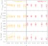 |
Fig. 21 Comparison between the median ages, metallicities, velocity dispersions and dust extinction derived from median stacked spectra (open circles) and individual spectra (open triangles) in the case of BC03 models (vertical bars are the MADs on the results from individual spectra) for the two mass bins 11.25 < log (M/M⊙) < 11.5 (left) and log (M/M⊙) > 11.5 (right). |
6. The question of progenitors
Linking galaxies at z ~ 0 with their progenitors back in cosmic time is essential to derive a coherent evolutionary pattern and understand the formation process of different galaxy types. In this work, we attempt to place constraints on the progenitors of nearby (z ≲ 0.3), very massive (log (M/M⊙) > 10.75) and passive ETGs by exploiting their SFH, reconstructed from the full spectrum fitting analysis described in previous sections. The aim is to verify if the inferred properties of the progenitors fit into an evolutionary path consistent with other observational constraints. In this regard, we first infer the properties of the star-forming progenitors from which today’s massive ETGs originated, and then follow their evolution until they terminate the star formation activity and become quiescent descendants at later cosmic times.
As we have already mentioned, our method is not able to distinguish if the analyzed massive and passive galaxies formed with a monolithic-like collapse at high redshift or if coeval mergers occurred to build their stellar mass. In this regard, it is important to clarify that the results described in the following sections implicitly assume that no coeval merger events have happened during the formation history of the analyzed galaxies. Furthermore, we illustrate the results derived assuming the Expdelc as the parametric form describing the observed SFHs.
6.1. The star-forming progenitor phase
Starting from the shapes of the SFHs illustrated in Sect. 4.4 (Fig. 16), we display the inferred evolutionary path of our sample ETGs in the SFR – stellar mass plane. Figure 22 shows the evolutionary tracks separately for the four mass bins of our sample as a function of cosmic time, together with the main sequences (MS) of star-forming galaxies available in the literature as a function of redshift. All the MS relations have been normalized to the Chabrier (2003) IMF adopted in this work.
Several important results emerge from Fig. 22 (which illustrates the case of BC03 models). The inferred SFRs were high in the past, with typical levels ⟨ SFR ⟩ 68% up to 350−400M⊙yr-1 for the most massive bin, but broadly consistent with those of MS galaxies at the same redshifts and masses. At early epochs (z ~ 3−6), the SFRs increase with mass and, for a given redshift, the slope of the SFR–mass correlation is similar to that of the MS. An example is represented by the comparison with the results of Salmon et al. (2015), who used CANDELS data to derive the MS relation at 3.5 ≲ z ≲ 6. Our results suggest that the progenitors of our ETGs were already forming stars at very high rates at z> 3−4. Such early formation epochs (3 ≲ z ≲ 10) are also derived by McDermid et al. (2015) for ATLAS3D ETGs with masses comparable to those of our sample. Fig. 22 also shows that after ~400 Myr, the SFRs of our ETGs decrease rather rapidly to a few M⊙yr-1 at z ~ 2, and that this tends to occur slightly earlier for the galaxies in the highest mass bin (where a deviation from the slope of the SFR – mass relation is present). Complete quiescence is achieved at later cosmic times. In particular, if the SFR at which a galaxy of a given mass is considered quiescent is defined as SFR(M) ~ 10-11yr-1 · M/M⊙, our sample ETGs become inactive at z ~ 1.5−2.
These evolutionary trends are apparent in the complementary Fig. 23, which illustrates the specific star-formation rate (sSFR, i.e. SFR per unit mass) for the four mass bins as a function of look-back time, together with the literature values (derived from the SFRs of Fig. 22). This shows that the peak of star-formation activity of the very massive and passive ETGs occurred at 4 ≲ z ≲ 7. MS11 models provide a similar evolution for the sSFR at z> 6 (with SFR up to ~700–750 M⊙yr-1), even if a steepening with respect to the BC03 predictions occurs at lower redshifts, suggesting slightly higher redshifts for the beginning of the quiescent phase (z ~ 1.5−2).
Either case, we find that the studied galaxies have already formed ≳75% (i.e. M ≳ 1010.62 M⊙) of the total stellar mass by  , thus we expect their progenitors at this redshift to be also very massive – in the hypothesis of no coeval mergers. If these systems are dusty and follow the same star-formation scaling relations present at lower redshifts, the inferred SFRs imply infrared luminosities in the range of the so called luminous to ultra-luminous infrared galaxies (11 ≲ log (LIR/L⊙) ≲ 13).
Clearly, the question is whether galaxies with very high SFRs and substantial stellar masses have been observed at such high redshifts (if no mergers occurr). The answer is probably yes, although the information is still limited and fragmentary. Examples are represented by high redshift millimeter/submillimeter galaxies at z ~ 4−5 (Schinnerer et al. 2008; Daddi et al. 2009; Hodge et al. 2015) and massive starbursts at z ~ 5−6.3 (Walter et al. 2012; Riechers et al. 2013, 2015). Also the existence of galaxies at z> 3 with simultaneous substantial stellar masses and high SFRs is suggestive of systems that could evolve rapidly towards a quiescence phase (Béthermin et al. 2015; see also Pozzi et al. 2015). In this regard, the massive and mostly quenched galaxies at z ~ 3 discovered by Taniguchi et al. (2015) could also fit well into a scenario of earlier star formation as inferred from the SFHs of our sample of ETGs. Last but not least, the mere existence of QSOs at z ~ 6 with massive and evolved host galaxies (e.g. Fan et al. 2003; Dietrich et al. 2003; Freudling et al. 2003; Goto et al. 2009; Bañados et al. 2014; Wu et al. 2015) may be consistent with this scenario.
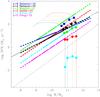 |
Fig. 22 Evolving SFR – mass curves (in the case of BC03 models and for the Expdelc parametric form). The four dotted curves are the evolving SFR – mass relations for the four mass bins of our sample (deduced from the SFHs of Fig. 16) as a function of cosmic time (from left to right), colour coded as in Fig. 16. Blue, black, green, red, cyan and magenta lines are the SFR – mass relations deduced by different authors at various redshifts (as indicated in the top left of the figure), within their observed mass ranges (solid lines). Filled circles are the SFR for the four mass bins at various z, corresponding to the ones reported in the top left of the figure (we note that, at z ~ 0, we derive log (SFR) < −3, thus the values at this redshift are not included in the plot). The grey dashed-dotted line represents the level of SFR at which the galaxies can be considered completely quiescent. |
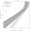 |
Fig. 23 Evolving sSFR−z relations for the Expdelc parametric form. Solid and dotted curves are the sSFR−z relations for the four mass bins (colour coded as in Fig. 16) for BC03 and MS11 models, respectively. Blue, black, green, cyan and red open circles (and violet open triangle) are the sSFR estimates obtained by various authors at different redshifts (for the four mass bins), as indicated in the top left of the figure. The grey horizontal dashed-dotted line marks the level of sSFR at which a galaxy is in general considered completely quiescent (sSFR ≲ 10-11 yr-1). Dark-grey and light-grey shaded regions represent the uncertainty on the look-back time, associated with the results from BC03 and MS11 models, respectively. |
6.2. The quiescent descendent phase
According to the inferred SFHs (Fig. 16), the progenitors of our sample ETGs are expected to be already quiescent by z ~ 1.5−2 (z ~ 2.5−3 in the case of MS11 models), with this phase lasting without other major episodes of star formation at later cosmic epochs. This implies that a population of massive and passive galaxies (M ≳ 1010.75 M⊙) should already be in place at z ~ 2−4.
Such galaxies have indeed been spectroscopically identified up to z ~ 3 (Dunlop et al. 1996; Cimatti et al. 2004; McCarthy et al. 2004; Kriek et al. 2006; Gobat et al. 2012), and subsequently studied in more detail (e.g. Cimatti et al. 2008; Saracco et al. 2009; Onodera et al. 2015; Belli et al. 2015; Lonoce et al. 2015; see also Newman et al. 2015). Their properties are broadly consistent with those expected in the evolutionary scenario inferred in this work. As a matter of fact, these galaxies are massive (M ~ 1010.5−11 M⊙), dominated by old stars (≳1 Gyr), passive or weakly star-forming, with low sSFR, and characterized by spheroidal morphologies and surface brightness profiles typical of early-type galaxies. However, at fixed mass their sizes are, on average, smaller than in present-day ETGs, implying a substantially higher stellar mass density (Daddi et al. 2005; Cimatti et al. 2008, 2012; Trujillo et al. 2011).
The archaeological results of our work imply that if complete quiescence is achieved by  (
( for MS11 models) on average, nearly quiescent galaxies (sSFR ~ 10-11 yr-1, up to 10-10 yr-1) should be present also at higher redshifts. This possibility is now strongly supported by the detection of several massive quiescent galaxy candidates at 3 <z< 7 (Mobasher et al. 2005; Rodighiero et al. 2007; Wiklind et al. 2008; Mancini et al. 2009; Fontana et al. 2009; Brammer et al. 2011; Muzzin et al. 2013; Straatman et al. 2014; Caputi et al. 2015; Marsan et al. 2015). Although these galaxies are too faint for the current spectroscopic sensitivity, their photometric SEDs suggest that they are massive (up to M ~ 1011 M⊙), old (often with ages close to the age of the Universe at their redshifts) and have low sSFRs. We note that the existence of massive galaxies at high redshifts is also a crucial test for the structure formation in the ΛCDM cosmological context (Steinhardt et al. 2015).
6.3. The size of the progenitors
More information comes from the sizes of our passive ETGs. Figure 24 shows a comparison between the effective radii Re of the analyzed galaxies and those of the parent population, which we define as the ensamble of SDSS DR4 ETGs with log (M/M⊙) > 10.75 (Kauffmann et al. 2003)8. In particular, Re are taken from the NYU Value-Added Galaxy catalogue (Blanton et al. 2005). Moreover, since the majority of our passive, massive ETGs are bulge-dominated systems (see Sect. 3), we restrict this analysis only to galaxies with this kind of morphology, both in the passive and the parent sample.
Figure 24 shows that the median Re increases for increasing mass (from ~5 Kpc to ~20 Kpc) and, given a stellar mass, our passive ETGs have median sizes smaller than those of the parent sample even by ~15% (at the highest masses). Furthermore, the entire Re distribution is extended to smaller radii in the case of passive ETGs, especially for log (M/M⊙) ≳ 11.5. Remembering that small differences in galaxy size imply large differences in stellar mass density, the derived trends suggest that the ETGs analyzed in this work should have formed from higher density progenitors which, in the hypothesis of no coeval mergers, do not increase their mass during the evolution. On the other hand, we cannot exclude the possibility that galaxies in the parent sample have experienced more dry mergers than our massive and passive galaxies, which have increased their size across cosmic time (Naab et al. 2009; Johansson et al. 2012a). The observed trend is also in agreement with some literature studies at low redshift which also suggest that more compact galaxies contain older stellar populations than larger ones (e.g. Saracco et al. 2009; Shankar & Bernardi 2009; Williams et al. 2010; Poggianti et al. 2013; McDermid et al. 2015). In general, this is qualitatively consistent with the high zF inferred by our analysis (z> 5) since, according to the cosmological evolution of the baryonic matter density, gas was denser at these cosmic epochs. These findings also agree with recent observations of compact systems (with various level of SF) at z ~ 2−3, which could be identified as local massive ETGs progenitors (e.g. Daddi et al. 2004; Cattaneo et al. 2013; Finkelstein et al. 2013; Marchesini et al. 2014; Nelson et al. 2014; Williams et al. 2015). Moreover, recent models of elliptical galaxy formation also predict the formation of compact and dense progenitors at high redshifts (e.g. Johansson et al. 2012a; Naab et al. 2014 and references therein).
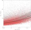 |
Fig. 24 Size – mass relation derived for our sample of massive, passive ETGs (red) and for the parent sample of local galaxies with log (M/M⊙) > 10.75 (grey) (Kauffmann et al. 2003 stellar masses are rescaled to the M11 ones). Colored points represent the two samples; solid curves are the P50 of the Re distribution at each mass. The dashed red curves and the shaded grey region includes the 68% of the Re distribution of the passive and the parent sample, respectively. |
6.4. The number density of progenitors
The number density (ρn) of our ETGs can be used as another consistency check in the comparison between the low redshift galaxy population and their progenitors at earlier epochs. To do that, we first derived the mass function (MF) of the analyzed galaxies at z ~ 0 by rescaling the local Baldry et al. (2008) MF9 (of all galaxy types) to the percentage of galaxies of each mass bin towards the parent population (which increases from ~23% to ~70% from the lowest to the highest masses ), which is defined as in the previous section, but now includes galaxies of any morphology. Then, we evolve this local MF back in cosmic time following the decrease of the stellar mass predicted by the derived SFHs, inferring, at each cosmic time, the number density of galaxies above log (M/M⊙) = 10.75. We verified that the mass completeness of our subsample of massive and passive galaxies is consistent with that of the global sample of galaxies above log (M/M⊙) = 10.75 and at z ≲ 0.3, on which the Vmax correction was already applied (see Baldry et al. 2008), and that our mass subsamples show no significant mass evolution as a function of redshift. At z ~ 0, we obtain log (ρn) ~ −3.98 ± 0.1 Mpc-3.
Figure 25 shows a comparison between the ρn obtained from this procedure and the literature10, as a function of both the look-back time and the spectral synthesis models used for the fit (BC03 and MS11 models). In the case of BC03 models we find that when the analyzed ETGs are completely quiescent and have already formed the totality of their stellar mass (0 ≲ z ≲ 2), the ρn inferred by us is independent of look-back time and is compatible with the literature, not exceeding the total number of passive galaxies per unit volume observed above the same mass threshold. Moreover, the redshift at which we have no more quiescent galaxies (since they are turning into star-forming systems, z ~ 2) is consistent with the one at which the ρn of quiescent galaxies observed in literature starts to rapidly decline. At earlier epochs, when the ETGs are still forming stars, the ρn of the SF progenitors starts to turn down, as the stellar mass formed by the ETGs decreases, and its value at 2 ≲ z ≲ 3 (i.e. log (ρn) ~ −4.1 Mpc-3) is in agreement with the literature observations at the same redshifts. Towards the beginning of the SF (z> 3), ρn rapidly decreases and, within the uncertainty on the look-back time (±0.6 Gyr, see Table 4), this decline is in agreement with the one observed in the literature for the global population of SF and quiescent galaxies.
In the case of MS11 models, the drop of ρn occurs at slightly earlier times due to the shorter derived SFH. However the results are also in this case in agreement with the low redshift observations and marginal consistency with the literature is still present at high z.
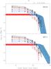 |
Fig. 25 Number density above log (M/M⊙) = 10.75. The central coloured bands are the ρn of the ETG progenitors as a function of the look-back time in the case of BC03 (upper panel) and MS11 (lower panel) models, derived from the SFHs of the analyzed ETGs, together with its uncertainty (±0.1 dex) and the uncertainty on the look-back time (i.e. |

Finally, for each mass bin, we also calculate the star-formation rate density (SFRD) of the SF progenitors at z ~ 5 by multiplying the typical star formation rates ⟨ SFR ⟩ 68% defined in Sect. 6.1 by the ρn of the considered mass bin. From this, we infer a global SFRD log (SFRD)~−1.71 M⊙yr-1Mpc-3, which is totally consistent, within the uncertainties, with the Madau & Dickinson (2014) SFRD at the same redshift, which amounts to log (SFRD)~−1.72 ± 0.27 M⊙yr-1Mpc-3 (the uncertainties on the Madau & Dickinson (2014) SFRD are taken from Behroozi et al. 2013). However, in the case of MS11 models, a higher SFRD, that is log (SFRD)~−1.22 M⊙yr-1Mpc-3, is derived at the same redshift.
7. Summary and conclusions
In this work we analysed the median stacked spectra of a sample of 24 488 SDSS DR4 ETGs at z< 0.3 in order to derive the properties of their stellar populations and to reconstruct their star-formation histories. This study focused on the extreme cases of passive ETGs with the highest stellar masses (log (M/M⊙) > 10.75) which in turn represent the passive envelope of the galaxy population at 0 <z< 0.3. The sample was divided into four bins with increasing stellar mass. The stacked optical spectra were analysed by means of the full-spectrum fitting technique using the public code STARLIGHT in order to derive constraints in a way that is complementary to the traditional method of Lick indices based on a few absorption lines. Using this archaeological approach, we also inferred the properties of the progenitors of massive and passive ETGs. Our main results can be summarized as follows.
-
First of all, STARLIGHT was tested against stellar population synthesis models to assess its reliability in the case of spectra similar to those of ETGs. It was found that the software retrieves the stellar population main properties (age, metallicity, SFH, dust extinction) and the velocity dispersion with a percentage accuracy higher than 10% for S/N ≳ 10–20, even if more complex SFHs are considered. In order to minimize the uncertainties, the STARLIGHT analysis was applied to stacked spectra with typical S/N ~ 80.
-
Mass-weighted stellar ages are very old, increasing with cosmic time from ~10 to ~13 Gyr, and show a clear tendency to increase with mass despite the rather limited mass leverage of our sample, which is selected to include only the most massive systems (log (M/M⊙) > 10.75). This result provides an additional support to the downsizing evolutionary scenario where more massive galaxies are older than less massive ones. The derived ages are broadly compatible with those found with different full-spectrum fitting codes (e.g. McDermid et al. 2015 and Conroy et al. 2014) and with the Lick indices approach (e.g. Thomas et al. 2010; Graves & Schiavon 2008). The bottom line is that the most massive and passive ETGs represent the oldest galaxies in the present-day Universe, with ages close to the age of the Universe itself in the most extreme cases.
-
Mass-weighted metallicities are slightly supersolar, with a median Z ~ 0.029 ± 0.0015 (Z ~ 0.027 ± 0.0020 for MS11 models), increase with stellar mass, and do not show any significant trends with redshift. This supports the interpretation that the analyzed galaxies are very old objects which formed the bulk of their stars much earlier and did not enrich significantly their interstellar medium with new metals at later epochs (however, we remind readers that we have a limited leverage in cosmic time, i.e. ~3.3 Gyr). This contrasts with the metallicity evolution of star-forming galaxies (e.g. Maiolino et al. 2008; Mannucci et al. 2009; Foster et al. 2012; Zahid et al. 2013; De Rossi et al. 2015). Although our metallicities are broadly consistent with other results at a fixed stellar mass, a large scatter is present amongst the estimates of the metallicity (Z) obtained with different methods.
-
The SFHs inferred with the full-spectrum fitting suggest that the star formation occurred during an extended period of time. The SFHs are globally compatible with a parametric function of the form SFR(t) ∝ τ− (c + 1)tc exp(−t/τ), where the typical values of τ and c are always short, with τ decreasing from 0.8 to 0.6 Gyr (with a dispersion of ± 0.1) from lower to higher masses and c ~ 0.1 (with a dispersion of ±0.05) regardless of mass, reproducing the fast rise of the SFR at the beginning of the SFH. Other works highlighted a stronger dependence of the star-formation timescale on the mass (e.g. Thomas et al. 2010; McDermid et al. 2015).
-
Based on the inferred SFHs, we derive that the ETGs of our sample formed about 50% of their stellar mass at early epochs, that is on average at z ≳ 5 (which decreases to z ≳ 3 if the small 0.5 Gyr systematic introduced by median stacked spectra is taken into account). Moreover, the most massive galaxies formed it ~0.2 Gyr (~0.1 Gyr for MS11 models) before than less massive systems.
-
Low dust extinction (AV ≲ 0.2−0.25 mag) are required to fit the spectra. In addition, in the case of BC03 models, a trend is present showing that AV tends to decrease for increasing stellar mass. The reliability, significance and interpretation of this trend requires further analysis beyond the scope of this paper, but a qualitative interpretation may be that the most massive galaxies were able to “clear” their interstellar medium more efficiently probably due to more intense feedback processes resulting from star formation and/or AGN activity.
-
The stellar velocity dispersions 200 ≲ σ ≲ 300 km s-1 estimated with STARLIGHT are consistent with estimates by other groups within the uncertainties, and increase with stellar mass.
-
Based on the SFHs, we reconstructed the mass assembly history and the properties of the progenitors of the most massive ETGs of the present-day Universe, assuming that no coeval mergers have occurred during the evolution of the analyzed galaxies. The SFHs imply that these galaxies were vigorously forming stars and assembled large stellar masses (≳75% of the total stellar mass) by
, with SFR up to 50−370 M⊙yr-1 (SFR ~ 140−750 M⊙yr-1 for MS11 models). Possible star-forming progenitors with these characteristics have indeed been found in samples of galaxies at 4 <z< 6.5 selected in the submm/mm. The inferred SFHs also predict the existence of quiescent galaxies at 2 <z< 4 characterized by large stellar masses and low specific star formation rate. Galaxies with these properties have been spectroscopically identified at z ~ 2−3, and photometric candidates at higher redshifts also exist. -
The Re of our sample ETGs are significantly smaller than those of the parent sample of SDSS DR4 ETGs with log (M/M⊙) > 10.75. This implies higher stellar mass densities and suggests that they formed from high density progenitors.
-
Based on the number density of the analyzed galaxies in the present-day Universe (log (ρn) ~ −3.98 ± 0.1 Mpc-3), the inferred number densities of the progenitors are consistent with the literature, within the uncertainties. Moreover, the mean star formation rate density implied by the star-forming progenitors does not violate the Madau & Dickinson (2014) relation at high redshift (z ~ 5), in the case of BC03 models.
-
We find a good agreement among our results concerning ages, metallicities and SFHs and those obtained using the fit to individual spectral features (Lick indices) and α-elements abundances. We thus suggest the full-spectrum fitting to be a complementary and valid approach to derive the stellar population properties and the star formation histories of early-type galaxies.
More information is available on the website: www.starlight.ufsc.br
Our normalization wavelength is fixed at 5520 Å.
Given an ensemble of data Xi, the median absolute deviation is defined as: MAD = 1.48 × median( | Xi−median(Xi) |, see Hoaglin et al. (1983).
[α/ Fe] ≈ (1/5)−(1/6)·log Δt, see Thomas et al. (2005).
We convert the [Z/H] values given by Thomas et al. (2010) following the conversion of Caputo et al. (2001): log Z = [Z/H] −1.7.
Where ![Mathematical equation: \hbox{$\rm [MgFe]'=\sqrt{\rm Mgb~(0.72~Fe5270~+~0.28 Fe5335)}$}](/articles/aa/full_html/2016/08/aa27772-15/aa27772-15-eq317.png) and [Mg2Fe] = 0.6 Mg2 + 0.4 log (Fe4531 + Fe5015).
and [Mg2Fe] = 0.6 Mg2 + 0.4 log (Fe4531 + Fe5015).
More information are available on the website http://spectro.princeton.edu/
We rescaled the stellar masses of the parent population, estimated by Kauffmann et al. (2003), to M11 stellar masses, by subtracting 0.2 dex to the former.
We rescaled Baldry et al. (2008) stellar masses (which are derived from an average on four stellar mass estimates, which include the Kauffmann et al. 2003, ones) to those of M11.
The literature MF have been all rescaled to a Chabrier (2003) IMF and to BC03 stellar masses (M11 stellar masses rely on these spectral synthesis models).
Acknowledgments
The authors thank the anonymous referee for the useful comments and suggestions, which helped to improve the paper. We are grateful to Emanuele Daddi for useful discussion, Maria Cebrián for providing the effective radii from the NYU-VAGC catalogue and Helena Domínguez-Sánchez, Kenneth Duncan, Andrea Grazian, Chiara Mancini and Adam Muzzin for providing their mass functions. A.C. is also gratetful to Alfonso Veropalumbo for helpful discussion. We also acknowledge the support of the grant PRIN MIUR 2010 The dark Universe and the cosmic evolution of baryons: from current surveys to Euclid. Funding for the SDSS and SDSS-II has been provided by the Alfred P. Sloan Foundation, the Participating Institutions, the National Science Foundation, the US Department of Energy, the National Aeronautics and Space Administration, the Japanese Monbukagakusho, the Max Planck Society, and the Higher Education Funding Council for England. The SDSS Web Site is http://www.sdss.org/. The SDSS is managed by the Astrophysical Research Consortium for the Participating Institutions. The Participating Institutions are the American Museum of Natural History, Astrophysical Institute Potsdam, University of Basel, University of Cambridge, Case Western Reserve University, University of Chicago, Drexel University, Fermilab, the Institute for Advanced Study, the Japan Participation Group, Johns Hopkins University, the Joint Institute for Nuclear Astrophysics, the Kavli Institute for Particle Astrophysics and Cosmology, the Korean Scientist Group, the Chinese Academy of Sciences (LAMOST), Los Alamos National Laboratory, the Max-Planck-Institute for Astronomy (MPIA), the Max-Planck-Institute for Astrophysics (MPA), New Mexico State University, Ohio State University, University of Pittsburgh, University of Portsmouth, Princeton University, the United States Naval Observatory, and the University of Washington.
References
- Andredakis, Y. C., Peletier, R. F., & Balcells, M. 1995, MNRAS, 275, 874 [NASA ADS] [CrossRef] [Google Scholar]
- Bañados, E., Venemans, B. P., Morganson, E., et al. 2014, AJ, 148, 14 [NASA ADS] [CrossRef] [Google Scholar]
- Baldry, I. K., Glazebrook, K., & Driver, S. P. 2008, MNRAS, 388, 945 [NASA ADS] [Google Scholar]
- Barber, T., Meiksin, A., & Murphy, T. 2007, MNRAS, 377, 787 [NASA ADS] [CrossRef] [Google Scholar]
- Behroozi, P. S., Wechsler, R. H., & Conroy, C. 2013, ApJ, 770, 57 [NASA ADS] [CrossRef] [Google Scholar]
- Bell, E. F., & de Jong, R. S. 2001, ApJ, 550, 212 [NASA ADS] [CrossRef] [Google Scholar]
- Belli, S., Newman, A. B., & Ellis, R. S. 2015, ApJ, 799, 206 [NASA ADS] [CrossRef] [Google Scholar]
- Bender, R., Capaccioli, M., Macchetto, F., et al. 1993, in European Southern Observatory Conference and Workshop Proceedings, 45, eds. I. J. Danziger, W. W. Zeilinger, & K. Kjär, 3 [Google Scholar]
- Benson, A. J. 2012, New Astron., 17, 175 [Google Scholar]
- Béthermin, M., Daddi, E., Magdis, G., et al. 2015, A&A, 573, A113 [NASA ADS] [CrossRef] [EDP Sciences] [Google Scholar]
- Blanton, M. R., Schlegel, D. J., Strauss, M. A., et al. 2005, AJ, 129, 2562 [NASA ADS] [CrossRef] [Google Scholar]
- Boylan-Kolchin, M., Springel, V., White, S. D. M., Jenkins, A., & Lemson, G. 2009, MNRAS, 398, 1150 [NASA ADS] [CrossRef] [Google Scholar]
- Brammer, G. B., Whitaker, K. E., van Dokkum, P. G., et al. 2011, ApJ, 739, 24 [NASA ADS] [CrossRef] [Google Scholar]
- Bruzual, G., & Charlot, S. 2003, MNRAS, 344, 1000 [NASA ADS] [CrossRef] [Google Scholar]
- Bruzual, A. G., & Kron, R. G. 1980, ApJ, 241, 25 [NASA ADS] [CrossRef] [Google Scholar]
- Burstein, D., Faber, S. M., Gaskell, C. M., & Krumm, N. 1984, ApJ, 287, 586 [NASA ADS] [CrossRef] [Google Scholar]
- Calzetti, D. 2001, PASP, 113, 1449 [NASA ADS] [CrossRef] [Google Scholar]
- Cappellari, M., & Emsellem, E. 2004, PASP, 116, 138 [NASA ADS] [CrossRef] [Google Scholar]
- Caputi, K. I., Ilbert, O., Laigle, C., et al. 2015, ApJ, 810, 73 [NASA ADS] [CrossRef] [Google Scholar]
- Caputo, F., Marconi, M., Musella, I., & Pont, F. 2001, A&A, 372, 544 [NASA ADS] [CrossRef] [EDP Sciences] [Google Scholar]
- Carollo, C. M., Danziger, I. J., & Buson, L. 1993, MNRAS, 265, 553 [NASA ADS] [CrossRef] [Google Scholar]
- Cattaneo, A., Woo, J., Dekel, A., & Faber, S. M. 2013, MNRAS, 430, 686 [NASA ADS] [CrossRef] [Google Scholar]
- Chabrier, G. 2003, PASP, 115, 763 [NASA ADS] [CrossRef] [Google Scholar]
- Choi, J., Conroy, C., Moustakas, J., et al. 2014, ApJ, 792, 95 [NASA ADS] [CrossRef] [Google Scholar]
- Cicone, C., Maiolino, R., Sturm, E., et al. 2014, A&A, 562, A21 [NASA ADS] [CrossRef] [EDP Sciences] [Google Scholar]
- Cid Fernandes, R., Mateus, A., Sodré, L., Stasińska, G., & Gomes, J. M. 2005, MNRAS, 358, 363 [NASA ADS] [CrossRef] [Google Scholar]
- Cimatti, A., Pozzetti, L., Mignoli, M., et al. 2002, A&A, 391, L1 [NASA ADS] [CrossRef] [EDP Sciences] [Google Scholar]
- Cimatti, A., Daddi, E., Renzini, A., et al. 2004, Nature, 430, 184 [NASA ADS] [CrossRef] [PubMed] [Google Scholar]
- Cimatti, A., Daddi, E., & Renzini, A. 2006, A&A, 453, L29 [NASA ADS] [CrossRef] [EDP Sciences] [Google Scholar]
- Cimatti, A., Cassata, P., Pozzetti, L., et al. 2008, A&A, 482, 21 [NASA ADS] [CrossRef] [EDP Sciences] [Google Scholar]
- Cimatti, A., Nipoti, C., & Cassata, P. 2012, MNRAS, 422, L62 [NASA ADS] [CrossRef] [Google Scholar]
- Cimatti, A., Brusa, M., Talia, M., et al. 2013, ApJ, 779, L13 [NASA ADS] [CrossRef] [Google Scholar]
- Conroy, C. 2013, ARA&A, 51, 393 [NASA ADS] [CrossRef] [Google Scholar]
- Conroy, C., & van Dokkum, P. 2012, ApJ, 747, 69 [NASA ADS] [CrossRef] [Google Scholar]
- Conroy, C., Graves, G. J., & van Dokkum, P. G. 2014, ApJ, 780, 33 [NASA ADS] [CrossRef] [Google Scholar]
- Cowie, L. L., Songaila, A., Hu, E. M., & Cohen, J. G. 1996, AJ, 112, 839 [Google Scholar]
- Daddi, E., Cimatti, A., Renzini, A., et al. 2004, ApJ, 600, L127 [NASA ADS] [CrossRef] [Google Scholar]
- Daddi, E., Renzini, A., Pirzkal, N., et al. 2005, ApJ, 626, 680 [NASA ADS] [CrossRef] [Google Scholar]
- Daddi, E., Dannerbauer, H., Stern, D., et al. 2009, ApJ, 694, 1517 [Google Scholar]
- Davies, R. L., Sadler, E. M., & Peletier, R. F. 1993, MNRAS, 262, 650 [NASA ADS] [Google Scholar]
- De Lucia, G., Springel, V., White, S. D. M., Croton, D., & Kauffmann, G. 2006, MNRAS, 366, 499 [NASA ADS] [CrossRef] [Google Scholar]
- De Rossi, M. E., Theuns, T., Font, A. S., & McCarthy, I. G. 2015, MNRAS, 452, 486 [NASA ADS] [CrossRef] [Google Scholar]
- Dekel, A., Birnboim, Y., Engel, G., et al. 2009, Nature, 457, 451 [NASA ADS] [CrossRef] [PubMed] [Google Scholar]
- Dietrich, M., Hamann, F., Shields, J. C., et al. 2003, ApJ, 589, 722 [NASA ADS] [CrossRef] [Google Scholar]
- Domínguez Sánchez, H., Pozzi, F., Gruppioni, C., et al. 2011, MNRAS, 417, 900 [NASA ADS] [CrossRef] [Google Scholar]
- Dressler, A., Lynden-Bell, D., Burstein, D., et al. 1987, ApJ, 313, 42 [NASA ADS] [CrossRef] [Google Scholar]
- Dunlop, J., Peacock, J., Spinrad, H., et al. 1996, Nature, 381, 581 [NASA ADS] [CrossRef] [Google Scholar]
- Faber, S. M., Worthey, G., & Gonzales, J. J. 1992, in The Stellar Populations of Galaxies, eds. B. Barbuy, & A. Renzini, IAU Symp., 149, 255 [Google Scholar]
- Fabian, A. C. 2012, ARA&A, 50, 455 [NASA ADS] [CrossRef] [Google Scholar]
- Fan, X., Strauss, M. A., Schneider, D. P., et al. 2003, AJ, 125, 1649 [NASA ADS] [CrossRef] [Google Scholar]
- Finkelstein, S. L., Papovich, C., Dickinson, M., et al. 2013, Nature, 502, 524 [NASA ADS] [CrossRef] [Google Scholar]
- Fontana, A., Santini, P., Grazian, A., et al. 2009, A&A, 501, 15 [NASA ADS] [CrossRef] [EDP Sciences] [Google Scholar]
- Fontanot, F., De Lucia, G., Monaco, P., Somerville, R. S., & Santini, P. 2009, MNRAS, 397, 1776 [NASA ADS] [CrossRef] [Google Scholar]
- Förster Schreiber, N. M., Genzel, R., Newman, S. F., et al. 2014, ApJ, 787, 38 [NASA ADS] [CrossRef] [Google Scholar]
- Foster, C., Hopkins, A. M., Gunawardhana, M., et al. 2012, A&A, 547, A79 [NASA ADS] [CrossRef] [EDP Sciences] [Google Scholar]
- Freudling, W., Corbin, M. R., & Korista, K. T. 2003, ApJ, 587, L67 [NASA ADS] [CrossRef] [Google Scholar]
- Gallazzi, A., Charlot, S., Brinchmann, J., White, S. D. M., & Tremonti, C. A. 2005, MNRAS, 362, 41 [NASA ADS] [CrossRef] [Google Scholar]
- Gobat, R., Strazzullo, V., Daddi, E., et al. 2012, ApJ, 759, L44 [NASA ADS] [CrossRef] [Google Scholar]
- Goto, T., Utsumi, Y., Furusawa, H., Miyazaki, S., & Komiyama, Y. 2009, MNRAS, 400, 843 [NASA ADS] [CrossRef] [Google Scholar]
- Graves, G. J., & Schiavon, R. P. 2008, ApJS, 177, 446 [NASA ADS] [CrossRef] [Google Scholar]
- Grazian, A., Fontana, A., Santini, P., et al. 2015, A&A, 575, A96 [NASA ADS] [CrossRef] [EDP Sciences] [Google Scholar]
- Heavens, A., Panter, B., Jimenez, R., & Dunlop, J. 2004, Nature, 428, 625 [NASA ADS] [CrossRef] [PubMed] [Google Scholar]
- Henriques, B. M. B., White, S. D. M., Thomas, P. A., et al. 2015, MNRAS, 451, 2663 [NASA ADS] [CrossRef] [Google Scholar]
- Henriques, B. M. B., White, S. D. M., Thomas, P. A., et al. 2013, MNRAS, 431, 3373 [NASA ADS] [CrossRef] [Google Scholar]
- Hoaglin, D. C., Mosteller, F., & Tukey, J. W. 1983, Understanding robust and exploratory data anlysis (New York: John Wiley & Sons) [Google Scholar]
- Hodge, J., Riechers, D. A., Decarli, R., et al. 2015, in AAS Meet. Abst., 225, 251.11 [Google Scholar]
- Ilbert, O., Arnouts, S., McCracken, H. J., et al. 2006, A&A, 457, 841 [NASA ADS] [CrossRef] [EDP Sciences] [Google Scholar]
- Ilbert, O., Salvato, M., Le Floc’h, E., et al. 2010, ApJ, 709, 644 [NASA ADS] [CrossRef] [Google Scholar]
- Ilbert, O., McCracken, H. J., Le Fèvre, O., et al. 2013, A&A, 556, A55 [NASA ADS] [CrossRef] [EDP Sciences] [Google Scholar]
- Jimenez, R., Bernardi, M., Haiman, Z., Panter, B., & Heavens, A. F. 2007, ApJ, 669, 947 [NASA ADS] [CrossRef] [Google Scholar]
- Johansson, J., Thomas, D., & Maraston, C. 2012a, MNRAS, 421, 1908 [NASA ADS] [CrossRef] [Google Scholar]
- Johansson, P. H., Naab, T., & Ostriker, J. P. 2012b, ApJ, 754, 115 [NASA ADS] [CrossRef] [Google Scholar]
- Juarez, Y., Maiolino, R., Mujica, R., et al. 2009, A&A, 494, L25 [NASA ADS] [CrossRef] [EDP Sciences] [Google Scholar]
- Kauffmann, G., Colberg, J. M., Diaferio, A., & White, S. D. M. 1999, MNRAS, 303, 188 [NASA ADS] [CrossRef] [Google Scholar]
- Kauffmann, G., Heckman, T. M., White, S. D. M., et al. 2003, MNRAS, 341, 33 [NASA ADS] [CrossRef] [Google Scholar]
- Khochfar, S., & Silk, J. 2006, ApJ, 648, L21 [NASA ADS] [CrossRef] [Google Scholar]
- Kriek, M., van Dokkum, P. G., Franx, M., et al. 2006, ApJ, 649, L71 [NASA ADS] [CrossRef] [Google Scholar]
- Kroupa, P. 2001, MNRAS, 322, 231 [NASA ADS] [CrossRef] [Google Scholar]
- Le Borgne, J.-F., Bruzual, G., Pelló, R., et al. 2003, A&A, 402, 433 [NASA ADS] [CrossRef] [EDP Sciences] [Google Scholar]
- Lonoce, I., Longhetti, M., Maraston, C., et al. 2015, MNRAS, 454, 3912 [NASA ADS] [CrossRef] [Google Scholar]
- Lu, Y., Mo, H. J., Weinberg, M. D., & Katz, N. 2011, MNRAS, 416, 1949 [NASA ADS] [CrossRef] [Google Scholar]
- Madau, P., & Dickinson, M. 2014, ARA&A, 52, 415 [NASA ADS] [CrossRef] [Google Scholar]
- Magris, G., Mateu, P. J., Mateu, C., et al. 2015, PASP, 127, 16 [NASA ADS] [CrossRef] [Google Scholar]
- Maiolino, R., Nagao, T., Grazian, A., et al. 2008, A&A, 488, 463 [NASA ADS] [CrossRef] [EDP Sciences] [Google Scholar]
- Mancini, C., Matute, I., Cimatti, A., et al. 2009, A&A, 500, 705 [NASA ADS] [CrossRef] [EDP Sciences] [Google Scholar]
- Mannucci, F., Cresci, G., Maiolino, R., et al. 2009, MNRAS, 398, 1915 [NASA ADS] [CrossRef] [Google Scholar]
- Maraston, C., & Strömbäck, G. 2011, MNRAS, 418, 2785 [NASA ADS] [CrossRef] [Google Scholar]
- Maraston, C., Daddi, E., Renzini, A., et al. 2006, ApJ, 652, 85 [NASA ADS] [CrossRef] [Google Scholar]
- Maraston, C., Strömbäck, G., Thomas, D., Wake, D. A., & Nichol, R. C. 2009, MNRAS, 394, L107 [NASA ADS] [CrossRef] [Google Scholar]
- Maraston, C., Pforr, J., Renzini, A., et al. 2010, MNRAS, 407, 830 [NASA ADS] [CrossRef] [Google Scholar]
- Marchesini, D., Muzzin, A., Stefanon, M., et al. 2014, ApJ, 794, 65 [NASA ADS] [CrossRef] [Google Scholar]
- Marsan, Z. C., Marchesini, D., Brammer, G. B., et al. 2015, ApJ, 801, 133 [NASA ADS] [CrossRef] [Google Scholar]
- McCarthy, P. J., Le Borgne, D., Crampton, D., et al. 2004, ApJ, 614, L9 [NASA ADS] [CrossRef] [Google Scholar]
- McDermid, R. M., Alatalo, K., Blitz, L., et al. 2015, MNRAS, 448, 3484 [NASA ADS] [CrossRef] [Google Scholar]
- Mendel, J. T., Saglia, R. P., Bender, R., et al. 2015, ApJ, 804, L4 [NASA ADS] [CrossRef] [Google Scholar]
- Mobasher, B., Dickinson, M., Ferguson, H. C., et al. 2005, ApJ, 635, 832 [NASA ADS] [CrossRef] [Google Scholar]
- Moresco, M., Jimenez, R., Cimatti, A., & Pozzetti, L. 2011, J. Cosmol. Astropart. Phys., 3, 45 [NASA ADS] [CrossRef] [Google Scholar]
- Moresco, M., Pozzetti, L., Cimatti, A., et al. 2013, A&A, 558, A61 [NASA ADS] [CrossRef] [EDP Sciences] [Google Scholar]
- Moustakas, J., Coil, A. L., Aird, J., et al. 2013, ApJ, 767, 50 [NASA ADS] [CrossRef] [Google Scholar]
- Muzzin, A., Marchesini, D., Stefanon, M., et al. 2013, ApJ, 777, 18 [NASA ADS] [CrossRef] [Google Scholar]
- Naab, T., Khochfar, S., & Burkert, A. 2006, ApJ, 636, L81 [NASA ADS] [CrossRef] [Google Scholar]
- Naab, T., Johansson, P. H., & Ostriker, J. P. 2009, ApJ, 699, L178 [NASA ADS] [CrossRef] [Google Scholar]
- Naab, T., Oser, L., Emsellem, E., et al. 2014, MNRAS, 444, 3357 [NASA ADS] [CrossRef] [Google Scholar]
- Nelan, J. E., Smith, R. J., Hudson, M. J., et al. 2005, ApJ, 632, 137 [NASA ADS] [CrossRef] [Google Scholar]
- Nelson, E., van Dokkum, P., Franx, M., et al. 2014, Nature, 513, 394 [NASA ADS] [CrossRef] [Google Scholar]
- Newman, A. B., Belli, S., & Ellis, R. S. 2015, ApJ, 813, L7 [NASA ADS] [CrossRef] [Google Scholar]
- Onodera, M., Carollo, C. M., Renzini, A., et al. 2015, ApJ, 808, 161 [NASA ADS] [CrossRef] [Google Scholar]
- Pacifici, C., Kassin, S. A., Weiner, B., Charlot, S., & Gardner, J. P. 2013, ApJ, 762, L15 [NASA ADS] [CrossRef] [Google Scholar]
- Panter, B., Jimenez, R., Heavens, A. F., & Charlot, S. 2007, MNRAS, 378, 1550 [NASA ADS] [CrossRef] [Google Scholar]
- Papovich, C., Dickinson, M., & Ferguson, H. C. 2001, ApJ, 559, 620 [NASA ADS] [CrossRef] [Google Scholar]
- Parkinson, D., Riemer-Sørensen, S., Blake, C., et al. 2012, Phys. Rev. D, 86, 103518 [NASA ADS] [CrossRef] [Google Scholar]
- Perlmutter, S., Aldering, G., Goldhaber, G., et al. 1999, ApJ, 517, 565 [NASA ADS] [CrossRef] [Google Scholar]
- Pforr, J., Maraston, C., & Tonini, C. 2012, MNRAS, 422, 3285 [NASA ADS] [CrossRef] [Google Scholar]
- Planck Collaboration XIII. 2016, A&A, in press, DOI: 10.1051/0004-6361/201525830 [Google Scholar]
- Poggianti, B. M., Calvi, R., Bindoni, D., et al. 2013, ApJ, 762, 77 [NASA ADS] [CrossRef] [Google Scholar]
- Pozzetti, L., Bolzonella, M., Zucca, E., et al. 2010, A&A, 523, A13 [NASA ADS] [CrossRef] [EDP Sciences] [Google Scholar]
- Pozzi, F., Calura, F., Gruppioni, C., et al. 2015, ApJ, 803, 35 [NASA ADS] [CrossRef] [Google Scholar]
- Ravindranath, S., Ferguson, H. C., Conselice, C., et al. 2004, ApJ, 604, L9 [NASA ADS] [CrossRef] [Google Scholar]
- Renzini, A. 2006, ARA&A, 44, 141 [NASA ADS] [CrossRef] [Google Scholar]
- Riechers, D. A., Bradford, C. M., Clements, D. L., et al. 2013, Nature, 496, 329 [Google Scholar]
- Riechers, D. A., Stacey, G., Giovanelli, R., et al. 2015, IAU General Assembly, 22, 55781 [NASA ADS] [Google Scholar]
- Riess, A. G., Filippenko, A. V., Challis, P., et al. 1998, AJ, 116, 1009 [NASA ADS] [CrossRef] [Google Scholar]
- Rodighiero, G., Cimatti, A., Franceschini, A., et al. 2007, A&A, 470, 21 [NASA ADS] [CrossRef] [EDP Sciences] [Google Scholar]
- Saglia, R. P., Maraston, C., Greggio, L., Bender, R., & Ziegler, B. 2000, A&A, 360, 911 [NASA ADS] [Google Scholar]
- Salmon, B., Papovich, C., Finkelstein, S. L., et al. 2015, ApJ, 799, 183 [NASA ADS] [CrossRef] [Google Scholar]
- Sánchez-Blázquez, P., Peletier, R. F., Jiménez-Vicente, J., et al. 2006, MNRAS, 371, 703 [NASA ADS] [CrossRef] [Google Scholar]
- Saracco, P., Longhetti, M., & Andreon, S. 2009, MNRAS, 392, 718 [NASA ADS] [CrossRef] [Google Scholar]
- Schawinski, K., Thomas, D., Sarzi, M., et al. 2007, MNRAS, 382, 1415 [NASA ADS] [CrossRef] [Google Scholar]
- Schinnerer, E., Carilli, C. L., Capak, P., et al. 2008, ApJ, 689, L5 [Google Scholar]
- Sersic, J. L. 1968, Atlas de galaxias australes (Córdoba, Argentina: Observatorio Astronómico) [Google Scholar]
- Shankar, F., & Bernardi, M. 2009, MNRAS, 396, L76 [NASA ADS] [CrossRef] [Google Scholar]
- Shapley, A. E., Steidel, C. C., Erb, D. K., et al. 2005, ApJ, 626, 698 [NASA ADS] [CrossRef] [Google Scholar]
- Springel, V., White, S. D. M., Jenkins, A., et al. 2005, Nature, 435, 629 [NASA ADS] [CrossRef] [PubMed] [Google Scholar]
- Stark, D. P., Ellis, R. S., Bunker, A., et al. 2009, ApJ, 697, 1493 [NASA ADS] [CrossRef] [Google Scholar]
- Steinhardt, C. L., Capak, P., Masters, D., & Speagle, J. S. 2016, ApJ, 824, 1 [NASA ADS] [CrossRef] [Google Scholar]
- Straatman, C. M. S., Labbé, I., Spitler, L. R., et al. 2014, ApJ, 783, L14 [NASA ADS] [CrossRef] [Google Scholar]
- Taniguchi, Y., Kajisawa, M., Kobayashi, M. A. R., et al. 2015, ApJ, 809, L7 [NASA ADS] [CrossRef] [Google Scholar]
- Thomas, D., Maraston, C., & Bender, R. 2003, MNRAS, 343, 279 [NASA ADS] [CrossRef] [Google Scholar]
- Thomas, D., Maraston, C., Bender, R., & Mendes de Oliveira, C. 2005, ApJ, 621, 673 [NASA ADS] [CrossRef] [Google Scholar]
- Thomas, D., Maraston, C., Schawinski, K., Sarzi, M., & Silk, J. 2010, MNRAS, 404, 1775 [NASA ADS] [Google Scholar]
- Tojeiro, R., Wilkins, S., Heavens, A. F., Panter, B., & Jimenez, R. 2009, ApJS, 185, 1 [NASA ADS] [CrossRef] [Google Scholar]
- Tojeiro, R., Masters, K. L., Richards, J., et al. 2013, MNRAS, 432, 359 [NASA ADS] [CrossRef] [Google Scholar]
- Trager, S. C., Faber, S. M., Worthey, G., & González, J. J. 2000, AJ, 120, 165 [NASA ADS] [CrossRef] [Google Scholar]
- Tremonti, C. A., Heckman, T. M., Kauffmann, G., et al. 2004, ApJ, 613, 898 [NASA ADS] [CrossRef] [Google Scholar]
- Treu, T., Ellis, R. S., Liao, T. X., et al. 2005, ApJ, 633, 174 [NASA ADS] [CrossRef] [Google Scholar]
- Trujillo, I., Ferreras, I., & de La Rosa, I. G. 2011, MNRAS, 415, 3903 [NASA ADS] [CrossRef] [Google Scholar]
- van Dokkum, P. G. 2005, AJ, 130, 2647 [NASA ADS] [CrossRef] [Google Scholar]
- van Dokkum, P. G., & Franx, M. 1996, MNRAS, 281, 985 [NASA ADS] [CrossRef] [Google Scholar]
- van Dokkum, P. G., Whitaker, K. E., Brammer, G., et al. 2010, ApJ, 709, 1018 [NASA ADS] [CrossRef] [Google Scholar]
- Vazdekis, A., Ricciardelli, E., Cenarro, A. J., et al. 2012, MNRAS, 424, 157 [NASA ADS] [CrossRef] [Google Scholar]
- Walter, F., Decarli, R., Carilli, C., et al. 2012, Nature, 486, 233 [NASA ADS] [CrossRef] [Google Scholar]
- Whitaker, K. E., van Dokkum, P. G., Brammer, G., et al. 2013, ApJ, 770, L39 [NASA ADS] [CrossRef] [Google Scholar]
- White, S. D. M., & Frenk, C. S. 1991, ApJ, 379, 52 [NASA ADS] [CrossRef] [Google Scholar]
- Wiklind, T., Dickinson, M., Ferguson, H. C., et al. 2008, ApJ, 676, 781 [NASA ADS] [CrossRef] [Google Scholar]
- Wilkinson, D. M., Maraston, C., Thomas, D., et al. 2015, MNRAS, 449, 328 [NASA ADS] [CrossRef] [Google Scholar]
- Williams, R. J., Quadri, R. F., Franx, M., et al. 2010, ApJ, 713, 738 [NASA ADS] [CrossRef] [Google Scholar]
- Williams, C. C., Giavalisco, M., Lee, B., et al. 2015, ApJ, 800, 21 [NASA ADS] [CrossRef] [Google Scholar]
- Wise, M. W., & Silva, D. R. 1996, ApJ, 461, 155 [NASA ADS] [CrossRef] [Google Scholar]
- Worthey, G., Bianca Danilet, A., & Faber, S. M. 2013, VizieR Online Data Catalog: J/A+A/561/A36 [Google Scholar]
- Worthey, G., Faber, S. M., & Gonzalez, J. J. 1992, ApJ, 398, 69 [NASA ADS] [CrossRef] [Google Scholar]
- Worthey, G., Faber, S. M., Gonzalez, J. J., & Burstein, D. 1994, ApJS, 94, 687 [NASA ADS] [CrossRef] [Google Scholar]
- Wu, X.-B., Wang, F., Fan, X., et al. 2015, IAU General Assembly, 22, 51223 [NASA ADS] [Google Scholar]
- Zahid, H. J., Geller, M. J., Kewley, L. J., et al. 2013, ApJ, 771, L19 [NASA ADS] [CrossRef] [Google Scholar]
All Tables
Median shift and dispersion from the simulation of ETGs spectra, for S/N = 20 and 100 and BC03 spectral synthesis models.
Number of galaxies, statistical, evolutionary and physical properties of the four mass bins of our sample (in the case of BC03 models).
Uncertainties on ages, metallicities, velocity dispersions and dust extinction provided by the three different estimates described in the text (in the case of BC03 models).
All Figures
|
Fig. 1 Simulated spectra of a CSP at 13 Gyr from the onset of the SFH (exponentially delayed with τ = 0.3 Gyr), with solar metallicity and S/N 2, 5, 10, 20 and 30, increasing from bottom to top. For each S/N, the blue curve is the starting BC03 model used for the simulation, while the red curve is the simulated spectrum. The lower panel shows the behaviour of the S/N as a function of wavelength for a simulated spectra with S/N = 30 in the 6500–7000 Å window. |
| In the text | |
|
Fig. 2 Retrieved ages, metallicities, dust extinctions and velocity dispersions as a function of the mean S/N of the input spectra. Blue-filled circles represent the differences, averaged over all the computed simulations (i.e. 10×13 models), between the ouptut and the input mass-weighted ages, mass-weighted metallicities, dust extinctions and velocity dispersions (from top to bottom); blue vertical bars are the median absolute deviations (MAD) on all the computed simulations; grey points are the differences derived from each individual simulation; yellow shaded regions in each panel indicate the minimum S/N from which the accuracy of the input retrieving is better than 10%. |
| In the text | |
|
Fig. 3 Recovery of star formation histories. The four panels show a CSP at 3, 5, 7 and 11 Gyr from the onset of the SFH. Black vertical lines represent the exponentially delayed SFH (τ = 0.3 Gyr) assumed for the input spectra (rebinned according to the age step of our library models), while vertical lines represent the output SFH; horizontal arrows indicate the time from the beginning of the SF (i.e. 3, 5, 7 and 11 Gyr, respectively), while grey vertical lines mark the asymmetric age ranges around the SFH peak defined in the text for CSPs younger or older than 5 Gyr (i.e. [−1; + 0.5] and [−1.5; + 1], respectively). |
| In the text | |
|
Fig. 4 Recovery of star formation histories. The four panels show a CSP at 3, 5, 7, and 11 Gyr from the onset of the SFH. In the two top panels, red triangles indicate the median mass fractions retrieved within [−1; + 0.5] Gyr from the SFH peak; in the two bottom panels, they are the median mass fractions within [−1.5; + 1] Gyr (as described in the text). In all four panels, cyan circles are the median mass fractions relative to stellar populations younger than 0.5 Gyr, while red and cyan horizontal lines mark the expected mass fraction within the defined age ranges and below 0.5 Gyr, respectively. |
| In the text | |
|
Fig. 5 Retrieving of more complex SFH. Left panel: output SFH (pink curve) obtained when an input SFH (grey curve) including only a single CSP is considered; right panel: output SFH (pink curve) obtained when an input SFH (grey curve and vertical line) including a single CSP plus a later burst (which happens 6 Gyr after the main SF episode and contributing 5% to the total mass. |
| In the text | |
|
Fig. 6 Retrieving of more complex SFHs as a function of the age and the mass contribution of the later burst. Left panels show the output SFH (pink curves) obtained when the input SFH (grey curves and vertical lines) includes a single CSP plus a later burst happening 6 Gyr after the main SF episode and contributing in mass by 3, 5 and 10% (from top to bottom). Right panels show the output SFH (pink curves) obtained when the input SFH (grey curves and vertical lines) includes a single CSP plus a later burst of SF contributing 5% to the total mass, and happening 4, 6, or 8 Gyr after the main SF event (from top to bottom). |
| In the text | |
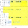 |
Fig. 7 As Fig. 2, but using the MS11 spectral library to retrieve the evolutionary properties. |
| In the text | |
|
Fig. 8 SDSS median stacked spectra for the sample of massive and passive ETGs. Left and right upper panels show, respectively, median stacked spectra with a fixed redshift (0.15 ≲ z ≲ 0.19) and different masses (with mass increasing from blue to red) and with a fixed mass (11.25 < log (M/M⊙) < 11.5) and four different redshifts (0.04, 0.08, 0.16, 0.23) (with redshift increasing from blue to red). Lower panels illustrate the fractional differences (defined as (fi−fREF/fREF) × 100, where fi is the flux of the ith spectrum and fREF is the reference flux) among the stacked spectra as a function of wavelength. In particular, to show the redshift and the mass dependence we used as reference, respectively, the median stacked spectrum obtained for 11.25 < log (M/M⊙) < 11.5 and 0.07 < z < 0.09, and the one corresponding to 10.75 < log (M/M⊙) < 11 and 0.15 < z < 0.17. Vertical grey lines mark some of the best-known absorption lines. |
| In the text | |
|
Fig. 9 Typical output of the full-spectrum fitting procedure using BC03 (left) and MS11 (right) spectral synthesis models. In particular, we show the case of the median stacked spectrum derived for 11 < log (M/M⊙) < 11.25 and z ~ 0.05. In the top panel the black curve is the observed spectrum, the red curve is the best fit model and grey shaded regions are the masked spectral regions (see Table 1). The bottom panel shows the ratio of the best fit model spectrum to the observed flux. |
| In the text | |
|
Fig. 10 Mass-weighted (top) and light-weighted (bottom) age-redshift relations (for BC03 models). Stellar mass increases from blue to red. The black line is the age of the Universe, while grey lines are the age of galaxies assuming different formation redshifts. |
| In the text | |
|
Fig. 11 Mass-weighted ages as a function of the velocity dispersion σ for BC03 models (symbols are colour-coded as in Fig. 10). Filled circles are the mass-weighted ages corresponding to z< 0.1, matching the redshifts analyzed by McDermid et al. (2015), with black curves linking the mass-weighted ages related to different mass bins but similar redshifts. The grey curve is the age – σ relation inferred by McDermid et al. (2015) with its dispersion (grey shaded region), while the light-blue curve is the Thomas et al. (2010) relation (its dispersion, not shown in the figure, is in the order of 60%). |
| In the text | |
|
Fig. 12 agef-redshift relations for the four mass bins. Solid and dotted curves (colour coded as in Fig. 10) are the ages of formation as a function of redshift referring, respectively to BC03 and MS11 spectral synthesis models. Dark-grey and light-grey shaded regions are the 1σ dispersions calculated starting from the 16th (P16) and 84th (P84) percentiles of the mass fraction cumulative function for BC03 and MS11 models, respectively. |
| In the text | |
|
Fig. 13 Mass fractions mj as a function of look-back time for the four mass bins, with mass increasing from top to bottom (in the case of BC03 models). Colored vertical lines (colour-coded as in Fig. 10) are the mj obtained from the full-spectrum fitting for each mass bin, put in phase according to their P50. In each mass bin, black vertical lines mark the P50 of the distribution, obtained from data as an average of the P50 of all the redshift bins, while black horizontal lines are the median dispersions [P50 – P16] and [P84 – P50]. The corresponding asymmetric Gaussians (grey) are overplotted on the mj distributions. On the top of the figure, the zF corresponding to each agef is indicated. |
| In the text | |
|
Fig. 14 Mass fractions mj recovered from the full-spectrum fitting as a function of redshift in the case of BC03 models. Red and blue curves refer, respectively, to stellar populations older and younger than 5 Gyr, with darker colours standing for higher stellar masses. |
| In the text | |
|
Fig. 15 SFHs derived from median stacked spectra. Mass increases from top to bottom, redshift increases from left to right, as indicated. Note that no significant episodes of SF occurred after the main SF event. The mass fractions relative to stellar population younger than 5 Gyr is very low (i.e. ≲5%). |
| In the text | |
|
Fig. 16 SFH for the four mass bins of our sample, with mass increasing from top to bottom (in the case of BC03 models). Colored vertical lines are the SFR (M⊙ yr-1) derived from the mj provided by the spectral fitting (colours are coded as in Fig. 10). In each mass bin, black vertical and horizontal lines are defined as in Fig. 13. In each panel, we show the two best fit models deriving from the assumption of an Expdel (dotted curves) or an Expdelc (solid curves) parametric function to describe the derived SFHs. The best fit parameters are also reported. Pink curves are the inverted-τ models with τ = 0.3 Gyr described in the text, extended up to 13.48 Gyr (which corresponds to the age of the Universe in the assumed cosmology). |
| In the text | |
|
Fig. 17 Mass weighted metallicities as a function of mass and redshift. Solid and dotted curves refer to BC03 and MS11 models, respectively. Stellar mass increases from blue to red, as indicated in the top right of the figure. |
| In the text | |
|
Fig. 18 Comparison between our mass-weighted metallicities (in the case of BC03 models) and the values reported in the literature. In particular, coloured filled circles (colour-coded as in Fig. 10) are our results (the cyan curve is a second order fit to our data); the grey curve is the scaling relation provided by Thomas et al. (2010), with its dispersion (grey shaded region), while black open circles and vertical bars are the measures (and dispersions) performed on our sample by Gallazzi et al. (2005). The light-brown curve is the relation derived by McDermid et al. (2015), together with its dispersion (light-brown shaded region). |
| In the text | |
|
Fig. 19 Velocity dispersions σ as a function of mass (for BC03 models). Colored triangles represent our observed values at different redshifts for each mass bin (the values of σ are illustrated together with the errors MAD/ |
| In the text | |
|
Fig. 20 Dust extinction AV as a function of redshift and mass. Solid and dotted curves refer to BC03 and MS11 models, respectively. Colors are coded as in Fig. 10. |
| In the text | |
|
Fig. 21 Comparison between the median ages, metallicities, velocity dispersions and dust extinction derived from median stacked spectra (open circles) and individual spectra (open triangles) in the case of BC03 models (vertical bars are the MADs on the results from individual spectra) for the two mass bins 11.25 < log (M/M⊙) < 11.5 (left) and log (M/M⊙) > 11.5 (right). |
| In the text | |
|
Fig. 22 Evolving SFR – mass curves (in the case of BC03 models and for the Expdelc parametric form). The four dotted curves are the evolving SFR – mass relations for the four mass bins of our sample (deduced from the SFHs of Fig. 16) as a function of cosmic time (from left to right), colour coded as in Fig. 16. Blue, black, green, red, cyan and magenta lines are the SFR – mass relations deduced by different authors at various redshifts (as indicated in the top left of the figure), within their observed mass ranges (solid lines). Filled circles are the SFR for the four mass bins at various z, corresponding to the ones reported in the top left of the figure (we note that, at z ~ 0, we derive log (SFR) < −3, thus the values at this redshift are not included in the plot). The grey dashed-dotted line represents the level of SFR at which the galaxies can be considered completely quiescent. |
| In the text | |
|
Fig. 23 Evolving sSFR−z relations for the Expdelc parametric form. Solid and dotted curves are the sSFR−z relations for the four mass bins (colour coded as in Fig. 16) for BC03 and MS11 models, respectively. Blue, black, green, cyan and red open circles (and violet open triangle) are the sSFR estimates obtained by various authors at different redshifts (for the four mass bins), as indicated in the top left of the figure. The grey horizontal dashed-dotted line marks the level of sSFR at which a galaxy is in general considered completely quiescent (sSFR ≲ 10-11 yr-1). Dark-grey and light-grey shaded regions represent the uncertainty on the look-back time, associated with the results from BC03 and MS11 models, respectively. |
| In the text | |
|
Fig. 24 Size – mass relation derived for our sample of massive, passive ETGs (red) and for the parent sample of local galaxies with log (M/M⊙) > 10.75 (grey) (Kauffmann et al. 2003 stellar masses are rescaled to the M11 ones). Colored points represent the two samples; solid curves are the P50 of the Re distribution at each mass. The dashed red curves and the shaded grey region includes the 68% of the Re distribution of the passive and the parent sample, respectively. |
| In the text | |
|
Fig. 25 Number density above log (M/M⊙) = 10.75. The central coloured bands are the ρn of the ETG progenitors as a function of the look-back time in the case of BC03 (upper panel) and MS11 (lower panel) models, derived from the SFHs of the analyzed ETGs, together with its uncertainty (±0.1 dex) and the uncertainty on the look-back time (i.e. |
| In the text | |
Current usage metrics show cumulative count of Article Views (full-text article views including HTML views, PDF and ePub downloads, according to the available data) and Abstracts Views on Vision4Press platform.
Data correspond to usage on the plateform after 2015. The current usage metrics is available 48-96 hours after online publication and is updated daily on week days.
Initial download of the metrics may take a while.