| Issue |
A&A
Volume 590, June 2016
|
|
|---|---|---|
| Article Number | A18 | |
| Number of page(s) | 16 | |
| Section | Extragalactic astronomy | |
| DOI | https://doi.org/10.1051/0004-6361/201527836 | |
| Published online | 28 April 2016 | |
Galaxy And Mass Assembly (GAMA): Improved emission lines measurements in four representative samples at 0.07 <z < 0.3
1
GEPI, Observatoire de Paris, CNRS, University Paris Diderot,
5 place Jules Janssen,
92195
Meudon,
France
e-mail:
This email address is being protected from spambots. You need JavaScript enabled to view it.
2
Australian Astronomical Observatory, PO Box 915, North Ryde, NSW
1670,
Australia
3
ICRAR,The University of Western Australia,
35 Stirling Highway,
Crawley, WA
6009,
Australia
4 Sydney Institute for Astronomy, School of Physics A28,
University of Sydney, NSW 2006, Australia
5
University of the Western Cape, Robert Sobukwe Road, Bellville, Cape Town
7535, South
Africa
6
Instituto de Astronomia, Universidad Nacional Autonoma de
Mexico, A.P. 70-264, 04510
Mexico, D.F.,
Mexico
7 Department of Physics and Astronomy, Macquarie University,
NSW 2109, Australia
8
Department of Physics and Mathematics, University of
Hull, Cottingham
Road, Kingston-upon-Hull, HU6
7RX, UK
9
School of Physics, Monash University, Clayton, VIC
3800,
Australia
10 School of Physics, the University of Melbourne, VIC 3010,
Australia
11
Astrophysics Research Institute, Liverpool John Moores
University, IC2, Liverpool Science
Park, 146 Brownlow Hill, Liverpool, L3
5RF, UK
12
Hamburger Sternwarte, Universität Hamburg,
Gojenbergsweg 112, 21029
Hamburg,
Germany
Received: 25 November 2015
Accepted: 14 March 2016
Abstract
This paper presents a new catalog of emission lines based on the GAMA II data for galaxies between 0.07 <z< 0.34. The catalog includes four subsamples containing 3000 galaxies drawn from the GAMA II survey and spanning four redshift windows. The four samples are representative of intermediate-mass galaxies down to log M∗> 9.4 at z ~ 0.1 and log M∗> 10.6 at z ~ 0.30. We have developed a dedicated code called MARVIN that automates the main steps of the data analysis, but imposes visual individual quality control of each measurement. We use this catalog to investigate how the sample selection influences the shape of the stellar mass – metallicity relation. We find that commonly used selection criteria on line detections and by AGN rejection could affect the shape and dispersion of the high-mass end of the M − Z relation. For log M∗> 10.6, common selection criteria reject about 65% of the emission-line galaxies. We also find that the relation does not evolve significantly from z = 0.07 to z = 0.34 in the range of stellar mass for which the samples are representative (log M∗> 10.6). For lower stellar masses (log M∗< 10.2) we are able to show that the observed 0.15 dex metallicity decrease in the same redshift range is a consequence of a color bias arising from selecting targets in the r-band. We highlight that this color selection bias affects all samples selected in r-band (e.g., GAMA and SDSS), even those drawn from volume-limited samples. Previously reported evolution of the M − Z relation at various redshifts may need to be revised to evaluate the effect of this selection bias.
Key words: galaxies: evolution / galaxies: ISM / galaxies: high-redshift
© ESO, 2016
1. Introduction
In the past two decades, large spectroscopic surveys have gathered spectra of millions of galaxies from the local Universe up to high-z. Notable examples include the Sloan Digital Sky Survey (SDSS) and the Galaxy And Mass Assembly (GAMA) at z ~ 0, the Canada France Redshift Survey (CFRS), and the Great Observatories Origins Deep Survey (GOODS) at higher redshift. Combined with multiwavelength photometry, redshift surveys have allowed us to constrain the evolution of the global density – luminosity, stellar mass, and star formation – up to high redshift. Given the homogeneity and quality of their data, large spectroscopic surveys are also an ideal tool for exploring the evolution of galaxy properties derived from emission line fluxes produced by the ionized interstellar medium (ISM) and absorption lines from stellar photospheres (e.g., Hammer et al. 1997; Brinchmann et al. 2004; Kauffmann et al. 2003b; Tremonti et al. 2004).
Larger samples reduce the adverse effects that are due to Poisson uncertainties, but they do not guarantee accuracy of measurements, which can still be affected by systematics. Flux and equivalent width measurements are highly sensitive to spectral quality and instrument residuals. In addition, obtaining highly accurate and precise measurements is challenging in samples of hundred thousands of galaxies. Several teams have improved the quality of emission and absorption measurements in the SDSS, such as MPIA-JHU1, Oh et al. (2011), or Juneau et al. (2014) for estimated uncertainties.
Summary of the GAMA data products collated in this work.
Sample selection is also a critical step for large surveys. Investigating the evolution of scaling relations or other key properties of galaxies requires linking samples at different epochs using a common physical parameter (Hammer et al. 2016). Stellar mass is particularly appropriate to define galaxy samples. The representativity of a sample and its mass-representativity limits can be assessed by comparing its mass distribution with the stellar mass function. Working with representative samples is also essential when investigating the demographics of subpopulations such as emission-line versus quiescent galaxies or galaxies hosting an active galactic nuclei, or evaluating the effect of additional selection criteria. Despite high completeness levels, magnitude-limited surveys (such as SDSS or GAMA at z ~ 0) are not representative samples when considering all galaxies in the observed volume. The single apparent magnitude criterion prevents us from detecting intrinsically faint galaxies at high redshift, while those galaxies would be included in the sample at low redshifts. While this selection effect (Malmquist bias) is always corrected for when investigating global density (e.g., Vmax method, Wall & Jenkins 2012) or environmental dependences, it is rarely taken into account when establishing scaling relations based on the same surveys. Salim et al. (2007) corrected the main-sequence M − star formation rate (SFR) for the Malmquist bias using a Vmax -weighted approach. Saulder et al. (2013) used a similar method to re-evaluate the fundamental plane. Another approach to avoid the Malmquist bias consists in defining volume-limited samples at various redshifts within the magnitude-limited survey. Foster et al. (2012) derived a local stellar mass – metallicity relation (M-Z) using volume-limited subsamples for the faint mr> 17.7 distribution from the GAMA II survey. Subsequently, Lara-López et al. (2013) expanded the analysis in a wide window of the Mr distribution by combining volume-limited samples extracted from both SDSS and GAMA.
In this work, we have constructed an emission line catalog for four representative samples gathered from GAMA II (Hopkins et al. 2013; Liske et al. 2015). The GAMA survey is a large multiwavelength photometric and spectroscopic galaxy survey (Driver et al. 2009, 2011), which aims to collect observations ranging from radio to ultraviolet wavelengths for about 300 000 galaxies over 280 square degrees. The GAMA survey is designed to achieve full spectroscopic completeness down to a magnitude limit of mr< 19.8. We have developed a dedicated software in IDL called MARVIN that is specially designed for the GAMA survey. It prevents the occurrence of systematics in line flux measurement from flux calibration or sky and instrumental residuals, and the occurrence of catastrophic measurements. MARVIN automates the main steps of the data analysis while still requiring visual quality control. Using this new emission line catalog, we derived the main properties of the ISM: extinction, SFR, and metallicity for star-forming galaxies. On the basis of these four representative samples, we have quantitively assessed the effect of selection criteria on the shape of the local stellar mass – metallicity relation, namely redshift cuts, simultaneous line detection, and AGN rejection. The paper is structured as follows: the GAMA survey and sample selection are described in Sect. 2. Section 3 presents our data analysis, while the performance of MARVIN is shown in Sect. 4. The representativity of the samples is discussed in detail in Sect. 5. The ISM properties of emission-line galaxies are presented in Sect. 6. Finally, Sect. 7 shows the results for the M − Z relation drawn from the four representative samples. In this section, we also discuss selection biases that affect the M − Z relation when it is established using non-representative samples. Throughout this work, we adopt a cosmology of H0 = 70 km s-1 Mpc-1, ΩM = 0.3 and ΩΛ = 0.7. We assume a Salpeter (1955) initial mass function (IMF).
2. Observations and sample selection
2.1. GAMA survey
GAMA is a unique sample to link the properties of local galaxies with those of distant galaxies. Taylor et al. (2011) have shown that the GAMA sample is complete to M∗ ~ 1010.5M⊙ at z ~ 0.25 and that the (g − i) color distribution is representative of the bulk of massive galaxies. The data are taken from the GAMA II spectroscopic sample (Hopkins et al. 2013; Liske et al. 2015). Several key physical properties are readily available, such as redshift (Driver et al. 2011), stellar mass (Taylor et al. 2011), and photometry (Hill et al. 2011), see Table 1. For every object with a secure spectroscopic redshift (i.e., nQ ≥ 32), aperture-matched photometry from optical to near-infrared was published by Hill et al. (2011) based on SDSS optical bands and near-infrared bands from the VIKING survey (Sutherland et al. 2015). This photometric catalog was used to derive stellar masses and absolute magnitudes in Taylor et al. (2011) through spectral energy distribution (SED) fitting. The stellar mass estimates assume the single stellar population models of Bruzual & Charlot (2003), a Chabrier (2003) IMF, and a Calzetti et al. (2000) extinction law.
The bulk of the GAMA spectra have been observed with the AAOmega spectrograph at the Anglo-Australian Telescope within 2 arcsec diameter fibers. The instrumental setup covers the 3700−8900 Å wavelength range with a spectral resolution of 3.2 Å. These observations and the quality of this dataset are described below. In addition to these dedicated observations, the GAMA survey has combined spectra from other redshift surveys overlapping with the GAMA fields. These include SDSS (Adelman-McCarthy et al. 2008), the six-degree Field Galaxy Survey (Jones et al. 2009) and the two-degree Field Galaxy Redshift Survey (Colless et al. 2001). We have restricted our analysis to flux-calibrated spectra (i.e., AAOmega and SDSS spectra only).
2.2. Definition of the sample: Mr selected
The present study aims to deliver a catalog of emission line fluxes for a subsample of GAMA for which the possible sources of systematics have been carefully controlled. Our method is to use a dedicated code that automates the main steps of the data analysis, but the quality control is done manually. We primarily aim to limit the occurrence of catastrophic measurements caused by failures of the data reduction and analysis process. While this method yields a drastic reduction in the systematic uncertainties, it is also extremely time consuming and can only be applied to a sample of moderate size. The choice of sample size is thus a trade-off between the gain in accuracy achieved with a semi-automated data analysis and the increase of the random uncertainty that is due to the decreasing number of targets. Each sub-ample should thus
-
1.
be representative of galaxies in that redshift window (i.e., theluminosity distribution of the sample should follow theluminosity function at the given redshift);
-
2.
have a moderate size to allow manual quality control of the data analysis; and
-
3.
be sufficiently large to ensure that the error budget is not dominated by small number statistics.
In this work, typical uncertainties associated with measurements of emission line ratios are on the order of 0.10 dex, or ~25%. The Poisson statistical uncertainty  in each bin should thus be smaller than 25%. This translates into at least 15 targets per bin. We target a minimum of five stellar mass bins at a given redshift to investigate the M − Z, hence the final redshift subsample should contain at least 75 galaxies. We chose to exceed this limit and used subsamples of ≳3000 targets to account for the fraction of red (non-star-forming) galaxies in the sample and the occurrence of problematic spectra. This increase on the sample translates into a decrease of the statistical uncertainty of lower than 10% in each stellar bin (<0.04 dex).
We defined four redshift subsamples from the three equatorial regions (G09, G12, and G15) of the GAMA II spectroscopic sample as follows: (0) 0.07 <z< 0.1; (1) 0.1 <z< 0.15; (2) 0.17 <z< 0.24; and (3) 0.24 <z< 0.30. The purpose of the redshift gap between samples (2) and (3) is to avoid the strong telluric lines overlapping with Hα . Only galaxies above z> 0.07 were selected to minimize fiber aperture problems (Kewley & Ellison 2008, scaled for the 2′′ GAMA fibers). Galaxies in our sample are required to have a reliable spectroscopic redshift (i.e., quality flag nQ = 4). In each redshift window, the range of r-band absolute magnitude Mr for which the sample is representative was determined as follows. The Mr distribution of the sample was compared to the luminosity function of Montero-Dorta & Prada (2009) based on the SDSS DR63. K-corrections and evolution corrections were applied to the local luminosity function in the higher redshift samples assuming the correction from Bell et al. (2003). The Mr limits for which the sample is representative were constrained using a two-tailed Kolmogorov-Smirnov (KS) test. We tested the Mr threshold for which the null hypothesis holds that the sample and the luminosity function arise from the same parent distribution. A standard confidence level of 95% (i.e. p = 0.05) was chosen for the rejection threshold. Given the large size of the GAMA sample, we were able to perform the KS test on 1000 subsamples of 3000 randomly drawn elements. The final four subsamples were randomly drawn from the main sample (StellarMasses catalog) according to the determined absolute r-band magnitude threshold for which GAMA is representative of galaxies as a whole within the appropriate redshift range (Fig. 1).
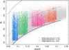 |
Fig. 1 Redshift versus Petrosian r-band absolute magnitude (Mr) for GAMA sources with reliable redshift and stellar mass estimates (gray dots). The four color boxes correspond to each of the stellar-mass-selected samples: 0.07 <z< 0.1 (blue), 0.1 <z< 0.15 (green), 0.17 <z< 0.2 (pink), and 0.2<z<0.3 (red), and are representative between −23 <Mr< − 18.4, −23 <Mr< − 19.2, −23 <Mr< − 20.4, and −23 <Mr< − 21, respectively. The dashed and dotted lines are the Mr limits corresponding to the apparent magnitude limits of the SDSS (mr> 14.5 for the bright limit and mr< 17.7). The black solid line indicates Mr limits corresponding to the apparent magnitude limits of GAMA (mr< 19.8). |
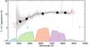 |
Fig. 2 Assessment of the spectrophotometric accuracy of the GAMA spectra. The flux-calibrated spectra (light gray line) are compared with the multiband photometry from SDSS (open red squares). The solid black line corresponds to a heavy smoothing of the spectrum, and the solid circles are the summed fluxes from the spectrum. Since the flux calibration is more problematic at the edges of the spectra, we have estimated two intermediate pseudo-bands ug and iz, in the AB system (λc = 4118 Å; 8206 Å), to be used as visual guidelines. We assume that the SED is roughly linear between the u and b-bands and between the i and z-bands. The fluxes in these two intermediate bands are estimated in the spectra by taking the median value around a small region of the central wavelength. |
3. Data analysis with MARVIN
This study includes spectra from two different spectrographs because GAMA targets with available SDSS spectra are not re-observed. The brighter targets tend to have SDSS spectra, and the two lowest redshift samples have the highest fractions of SDSS spectra. For the purposes of this work, we converted the SDSS spectra into the same file format as other GAMA spectra and performed the data analysis identically on both.
3.1. Data quality of the AAOmega spectra
GAMA spectra are obtained with the AAOmega spectrograph (Saunders et al. 2004; Smith et al. 2004; Sharp et al. 2006) on the 3.9 m AAT (Siding Spring Observatory, NSW, Australia). AAOmega possesses a dual beam system that allows a total coverage from 3750 to 8850 Å with the 5700 Å dichroic. The resolution varies as a function of wavelength from 3.4 Å in the blue arm to 5.5 Å in the red arm. After the 1D extraction of the spectrum, the blue and red spectra for each galaxy are spliced by doing a rough flux calibration to best match the spectra at the splice wavelength (5700 Å). The spectra are corrected for aperture losses by matching the spectrophotometry directly to the r-band Petrosian magnitudes measured by the SDSS photometry. A complete description of the observational setup and data reduction can be found in Hopkins et al. (2013). The final spectra have a pixel scale of 1 Å pixel-1 and the wavelength calibration is accurate to better than 0.1 Å. The flux calibration is typically accurate to 10−20%, although the reliability is worse at the extreme wavelength ends and poorer in the blue than the red. More critically, there is a bias of ~5% in the blue wavelength end that is due to the low instrumental response in this region. This issue is particularly problematic when using diagnostics in the blue region (e.g., [O ii] λ3727 and D4000) because systematics are propagated through to the derived quantities.
3.1.1. Flux calibration accuracy
The spectrophotometric accuracy is inhomogeneous in GAMA II and varies between plate configurations. Very many plates have excellent spectrophotometric accuracy, while other plates suffer from catastrophic failure of the flux calibration step. This is mainly due to instrument residuals in the standard star spectra. The improvement of the GAMA flux calibration accuracy is the focus of ongoing work. For our purposes, we verified the spectrophotometry in the subsamples, flagging spectra with spectrophotometric uncertainties larger than 40% (quadratic sum of the uncertainties in the g, r, and i-bands).
The spectrophotometry was evaluated by comparing the fluxes from the photometry in the g, r, and i-bands in the fiber aperture with the integrated spectral fluxes under the transmission curves of the respective filters, see Fig. 2. Fiber magnitudes were calculated for all GAMA plate positions using the SDSS DR7 (Abazajian et al. 2009) u, g, r, i, and z photometric data (collated by Hill et al. 2011).
3.1.2. Quality control I: instrumental residuals
A small fraction (~3%) of the AAOmega spectra are affected by either fringing or poor splicing (see Fig. 1 from Hopkins et al. 2013). To avoid systematics in our measurements arising from these instrumental residuals, we performed a first-level quality control of the spectra by visually inspecting all spectra. Spectra were classified into five categories: (1) good for a galaxy spectrum without instrumental residuals; (2) fringed for a spectrum with visible high-frequency oscillation in the continuum level (Fig. 3A); (3) poor splicing for a spectrum characterized by a dramatic change in the continuum level at the splice wavelength (Fig. 3C); (4) poor spectrophotometry (Fig. 3B) for spectrophotometric uncertainties larger than 40%, see Sect. 3.1.1; and (5) no signal (e.g., pure noise spectrum). In addition, we took advantage of this quality-control stage to visually identify Seyfert I active galactic nuclei (AGN) emission. These AGN hosts are easily recognizable by their broad hydrogen emission lines, as shown in Fig. 3D.
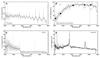 |
Fig. 3 Example spectra representing our four quality flags. Panel A) shows an example of a fringed spectrum. A spectrum with failed spectrophotometry is shown in panel B), wherein the red open squares are the fluxes estimated from the SDSS photometry inside the fibre aperture. Panel C) shows a spectrum with clear splicing problems around observed frame 5700 Å, where the blue and red spectra have been unsuccessfully joined. An example spectrum with broad hydrogen emission lines classified as Seyfert I is shown in panel D). |
We imposed stricter quality control criteria than in Hopkins et al. (2013) because our metallicity measurements are based on the measurements of line fluxes that are extremely sensitive to instrumental residuals. These measurements require spectra with good global and local spectrophotometry (the spectrophotometry and poor splicing criteria described above, respectively). According to our criteria, roughly a quarter of the GAMA spectra are potentially affected by instrumental residuals, see Table 2. The main difference between the Hopkins et al. (2013) quality control and that found here is the additional requirement on the spectrophotometry. Of the spectra rejected for this study, 71% failed because of the poor spectrophotometry. These spectra can be used to measure line positions and equivalent widths, but cannot be used to estimate quantities based on line fluxes. We also imposed a stricter criterion for poor splicing because metallicity estimates rely on the fluxes of the [O iii] and Hβ lines that fall in the splice region at the low redshifts of this study. By design, the quality flags are mutually exclusive even if the spectra may present more than one type of instrumental residual. For instance, poor spectrophotometry is usually correlated with poor splicing. The aim of our quality flagging is to reject spectra with instrumental residuals, and this consequently only provide a rough statistics on the occurrence of instrumental residuals in the AAOmega GAMA spectra. Only spectra that successfully passed the quality check are used in the analysis below.
After the first quality control, which removed spectra with strong instrumental residuals, the four samples contained 2633, 2747, 2101, and 2136 targets (including Seyfert I).
Summary table of the spectral quality flag statistics for the master sample.
3.2. Subtracting the stellar continuum
Accurate stellar continuum subtraction is essential for reliable measurements of emission line fluxes. This is particularly important for hydrogen recombination lines such as the Balmer lines, for which the emission line produced by the ionized gas is superimposed on the absorption line from the stellar photospheres. Not accounting for the underlying absorption when measuring emission lines leads to underestimating their flux and thus induces a bias in all subsequently derived properties (Kennicutt 1992; Liang et al. 2004; Moustakas & Kennicutt 2006).
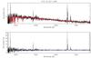 |
Fig. 4 Typical accuracy of the stellar continuum subtraction. Top panel: raw (gray), after correcting the low-frequency residuals (black) and synthetic spectra for a typical sample target. The correction of the low-frequency residuals are typically <5%. In this spectrum the correction is hardly visible. The correction is visible around 7000 Å, corresponding to a region typically affected by sky subtraction residuals. Lower panel: residuals after subtracting the synthetic spectrum. |
3.2.1. Methodology
For each spectrum, we modeled the stellar continuum using a linear combination of spectra from a grid of SSP models. The model spectra were first attenuated by a dust component and convolved for the measured stellar kinematics. Our grid of templates includes a set of 45 SSPs from Bruzual & Charlot (2003), which uses the Padova 1994 stellar evolutionary tracks and the STELIB empirical stellar library (Le Borgne et al. 2003). The SSP grid spans three metallicities (Z = 0.004, 0.02, and 0.05), 15 formation ages ranging from 10 Myr to 13 Gyr, and assumes a Chabrier initial mass function (Chabrier 2003) along with the Cardelli et al. (1989) extinction law (Rv = 3.1). We chose to use the models of Bruzual & Charlot (2003) instead of Charlot & Bruzual (2007; unpublished, updated of Bruzual & Charlot 2003) because although the newer models incorporate a better treatment of the thermally pulsating asymptotic giant branch (TP-AGB) stars, they lead to an underestimation of the stellar continuum around the Hβ line (Groves et al. 2012).
There are currently multiple software packages dedicated to full spectral fitting: MOPED (Heavens et al. 2000), PPXF (Cappellari & Emsellem 2004), PLATEFIT (Tremonti et al. 2004; Lamareille et al. 2006), STARLIGHT (Cid Fernandes et al. 2005), STECKMAP (Ocvirk et al. 2006), ULYSS (Koleva et al. 2009), and VESPA (Tojeiro et al. 2007). These are based on varying inversion methods and optimization algorithms, but according to the tests reported at the IAU Symposium 241, all give comparable results. We chose to use STARLIGHT (Cid Fernandes et al. 2005) to find the best-fit solution for each spectrum. The stellar population subtraction task in MARVIN is a wrapper to STARLIGHT. Our fitting procedure is divided into the following three main steps:
-
1.
The spectra are trimmed to excludeλobs< 4000 Å if the mean signal-to-noise ratio (S/N) is above 0.5% in this region. The blue region of the spectrum is next degraded to a spectral resolution of 5.5 Å to match the red spectrum resolution. The full spectrum is corrected for the foreground extinction using the maps of Schlegel et al. (1998) and finally set to rest frame.
-
2.
Low-frequency residuals are corrected for each spectrum. The full spectrum is first fit by masking regions with known instrumental features such as the splice region, bad pixels, and emission lines. This synthetic spectrum is then subtracted from the raw spectrum. The low-frequency component of this residual spectrum arises from imperfect sky-subtraction, instrumental residuals, or template mismatch. The residual spectrum is then smoothed using a wavelet decomposition, masking the emission lines, and is then subtracted from the input spectrum. This correction is added to the error budget of the spectrum. The typical fraction of correction is < 5%.
-
3.
Finally, the continuum of the corrected spectrum is fit with SSPs leaving all parameters to vary freely. Only bad pixels and regions with emission lines are masked in this step. The best-fit solution (red solid line in the upper panel of Fig. 4) is subtracted from the corrected spectrum, leaving a pure emission line spectrum (bottom panel of Fig. 4).
This procedure is applied to all spectra with mean S/N> 5 (S/N computed in the rest-frame window between 4000−4800 Å ). Below this S/N threshold, the subtraction of a synthetic stellar continuum is counter-productive since the uncertainties on the stellar continuum model are larger than the effect it aims to correct. In this case, the continuum is evaluated with a low-frequency wavelet fit to regions devoid of emission lines and noise spikes (rejected with a 3σ clipping).
3.2.2. Quality control II: continuum fit
The quality of the continuum fit is assessed by comparing the fit residuals rN with the expected statistical noise sN following Oh et al. (2011). A ratio close to one indicates a good fit. The mean ratio (rN/sN) for the 5709 galaxies above the S/N threshold is 1.01 with a small standard deviation of ~0.11, attesting to the high quality of stellar continuum subtraction. The small fraction of outliers (<15 spectra with rN/sN> 1.5) corresponds to low S/N spectra or spectra with unusually strong skyline residuals or moderate residuals in the splice region that evaded detection in quality control I (Sect. 3.1.2). Such high-quality fits are expected since the first quality control has already excluded spectra with obvious instrumental problems and the flux calibration correction performed in step 1 of the stellar continuum subtraction has significantly reduced low-frequency residuals.
3.3. Measuring emission lines
There is a tradeoff between the choice of S/N threshold necessary to ensure accurate flux measurements and potential systematics induced by selection effects. Our approach is to favor accuracy of the line measurements over systematics. However, a stringent selection in the significance of line detection does not inevitably imply selection effects since undetected lines can be taken into account as missing data or upper limits. Our approach is to (1) minimize the occurrence of false detections, (2) maintain a clear record of whether undetected lines are due to instrumental reasons (e.g., bad pixels, strong sky lines, and glitch), or are simply weaker than the S/N threshold, (3) minimize the systematics of the flux measurements in the low S/N regime. The architecture of the emission-line-fitting algorithm was designed to meet these three goals.
Emission lines from the warm ISM.
3.3.1. Fitting algorithm
The flux in the emission lines is measured by a simple Gaussian model and a first-order polynomial background using a Markwardt nonlinear least-squares curve-fitting algorithm (IDL routine MPFIT, Markwardt). Lines are fit in groups as defined in Table 3. Isolated emission lines with no nearby lines within 50 Å are fit individually. Close lines (e.g., Hα and the [N ii] lines) with possible blending are fit simultaneously, but with independent parameters for each line. Lines belonging to a doublet are fit simultaneously with the additional requirement of identical velocity dispersion. Each group is fit inside a spectral window ranging between −50 Å from the bluest line in the group and +50 Å from the reddest line in the group. Uncertainty vectors associated with the flux are taken into account during the fit, and bad pixels are flagged as missing data.
We imposed loose bounds on the values for the Gaussian parameters: continuum, center, width, and peak. The centers of the lines were allowed to be offset by ±5 Å relative to their reference wavelength to accommodate for small local mismatches in the wavelength calibration and uncertainties on the redshift. The line width was constrained to lie between 0.8 Å and 15 Å, which corresponds to 0.4−4.5 times the instrumental resolution. Since we are mainly interested in accurately evaluating the emission line fluxes, we preferred not to set boundaries on the ratio of line doublets to avoid truncated statistics. Ratios of line doublets could differ from the theoretical values for various reasons. The difference could be real if assumptions on the electron temperature of the gas, density, or escape fraction of the photons from the medium are different from the standard values, for example. It is also likely that the difference simply arises from artifacts such as data reduction residuals or poor estimation of the underlying stellar continuum. In the latter case, abnormal line ratios are a good indicator for the presence of systematics and measurements can thus be censored a posteriori.
Several levels of statistical tests are implemented within the algorithm to weed out false and failed detections. These include the evaluation of the fit quality through the χ2, a measure of the significance of the detection, rejection of measurements potentially affected by strong sky lines, and a posteriori censorship of line fits with unphysical parameters. The first criterion assesses the quality of the fit and is equivalent to a χ2 rejection test. The convergence of the χ2 minimization routine toward a solution does not imply, however, that a line has been successfully detected. We imposed two rejection criteria to identify false positives. We flagged as false positives all emission lines for which the relative uncertainty on the line fluxes (calculated from the Gaussian model) was larger than 70%. The second criterion evaluates the significance of the detection by testing against the null hypothesis that the signal is pure background noise. This is implemented by flagging lines with S/N< 5 as false detections following Rola & Pelat (1994). Rola & Pelat (1994) showed that an emission line can only be securely detected if the observed S/N is higher than 5 and that a S/N> 7 is required for a flux measurement sufficiently accurate to derive other quantities. As such, the line fluxes with 5 <S/N< 8 are upper limits, see discussion in the appendix on the S/N threshold. For each measured line, the S/N of detection (S / N)line was estimated as follows:  (1)where Fline is the line flux and σc is the level of the noise in the continuum around the groups of lines. Nline is the number of pixels spanned by the width of the line (i.e., 6 δd the mean velocity width of emission lines). Lines wider than 16 Å and lines that overlap with the [O i] λλ5577, 6302 strong sky emission lines are censored a posteriori as false detections.
The integrated line flux was estimated based on the parameters of the best-fit Gaussian model as follows. For unblended lines, we integrated the flux within ± 3σ of the center of the line. For blended lines, the flux under the Gaussian model is measured. The fluxes calculated by integrating directly and from the Gaussian model are consistent to within 5%. The associated 1σ statistical uncertainties were calculated by propagating the parameter uncertainties of the Gaussian fit. The median uncertainty on the fluxes are about 15% and 8% for faint lines, that is, 7 < (S/N)line< 12, in the blue and red CCD, respectively. In the high S/N regime ((S/N)line> 12) the typical uncertainties are 9% and 2% for lines in the blue and red CCDs, respectively. For galaxies without stellar continuum subtraction, the fluxes in the Balmer lines are lower limits since the underlying absorption could not be evaluated. For each undetected emission line, we estimated the upper limit on the line flux by assuming a Gaussian line-profile ( ).
).
3.3.2. Quality control III: reliability of emission line measurements
The quality of the fit was visually assessed for each emission line, see Fig. 5. We first verified the reliability of the algorithm to sucessfully detect emission lines. During this step, we first assessed the reliability of the emission line detection algorithm by registering the number of failed (< 0.05%) and false detections (< 0.04%). A failed detection corresponds to the non-detection of an emission line whose intensity is above the (S/N)line> 10 threshold. The reliability of MARVIN to detect lines is very good, with a failure lower than 0.1%.
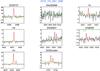 |
Fig. 5 Fitted emission lines for target G15-Y3-001-058 (also shown in Fig. 4). The input spectrum is shown as a black solid line. The red solid lines show the best fit to the emission lines and the green line corresponds to the weight given to pixels based on the flux uncertainties. Bad pixels and regions affected by strong sky lines have been rejected during the fit. Fitted lines with (S/N)line< 5 are rejected. |
4. Reliability of the emission line catalog
4.1. Internal consistency
We tested the internal consistency of the flux measurements by comparing the measured ratio of reference lines with their theoretical values. In the wavelength range of GAMA spectra, the [O iii] λλ4959, 5007 doublet is the ideal reference for such a test. Since the [O iii] doublet arises from a magnetic dipole transition, its intensity ratio can be theoretically predicted. Storey & Zeippen (2000) calculated a theoretical ratio of ~1 / 2.98. Figure 6 shows the distribution of the measured [O iii] doublet flux for 0.10 <z< 0.15 galaxies with (S/N)line> 7. The median flux ratio is 0.333, which is within 1 per cent of the theoretical value, and with a standard deviation of 0.07. At low S/N, the overestimation of the flux in the faintest line [O iii] λ4959 explains the log-normal shape of the distribution. The dispersion of the distribution agrees well with the mean uncertainty on the flux measurements at ~15% in the low S/N regime.
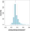 |
Fig. 6 Distribution of observed ratio of [O iii] λ4959/[O iii] λ5007 in 0.10 <z< 0.15 sample for S/Nline> 7. The solid arrow corresponds to the theoretical ratio of 1/2.98 (Storey & Zeippen 2000). The median and the 68th percentiles are represented as the dashed and dotted red lines, respectively. The median flux ratio is 0.333 with a standard deviation of 0.07, within 1 per cent of the theoretical value. |
We used the measurements of the [O iii] doublet lines fluxes to evaluate the limit to which our line fluxes are reliable (Brough et al. 2011). The flux limit corresponds to the flux where the ratio of the doublet is no longer accurate to within 10 per cent. For both AAOmega and SDSS spectra the flux limit is 4 × 10-16 ergs cm-2.
4.2. Comparision with GANDALF
Finally, we tested our flux measurements for systematics by comparing them with those previously measured using the GANDALF software (Hopkins et al. 2013). As for MARVIN, GANDALF measures the flux of emission lines after taking into account the underlying absorption from the stellar continuum. The main difference between the two codes is that GANDALF fits both Gaussian emission line and stellar population templates simultaneously. The GANDALF measurements of GAMA spectra are presented in Hopkins et al. (2013), wherein the stellar population templates of Maraston & Strömbäck (2011) and Calzetti et al. (2000) obscuration curve for the dust extinction in the stellar continuum have been assumed. Figure 7 shows the difference in the measured fluxes between the two algorithms. Outliers that are discrepant by more than 200% were not taken into account when computing the statistics. These outliers usually correspond to false detections in GANDALF: for sample 0.10 <z< 0.15, ~2.5% of the lines measured by GANDALF failed to pass MARVIN quality control. MARVIN fluxes are systematically 5% higher than those measured by GANDALF. The different stellar population templates (Bruzual & Charlot 2003 vs. Maraston & Strömbäck 2011) and obscuration curves, Cardelli et al. (1989) vs. Calzetti et al. (2000), are the likely origin for this small systematic offset. The difference between the two estimates is small at for (S/N)line> 10, but can be significant in the low S/N regime. As expected, the dispersion of flux differences for collisional lines is 15%, consistent with the respective flux uncertainties. Reassuringly, despite being very sensitive to the absorption correction, both methods give similar results for Balmer lines with systematic differences below 7%. The dispersion of measured differences for recombination lines in the blue is similar to the uncertainties.
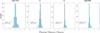 |
Fig. 7 Comparison between the flux measured by MARVIN and GANDALF for the spectra in sample 0.1 <z< 0.15. Only lines detected above a S/N threshold of 7 by both codes have been selected. Below this S/N threshold the fluxes are systematically overestimated, see discussion in the text. The false detections have been excluded in the comparison.The dashed and dotted lines are the median and standard deviation of the distributions, respectively. |
5. Sample properties
5.1. Representativity limits of the samples
In the upper panels of Fig. 8 we compare the stellar mass distribution of each subsample with the local stellar mass function from Baldry et al. (2012). The stellar masses were taken from Taylor et al. (2011) and an offset of +0.2 was applied to convert from a Chabrier into a Salpeter IMF. The ranges of stellar mass for which the samples are representative were estimated based on a Kolmogorov-Smirnov test between the stellar mass distribution and the stellar mass function at different stellar mass completeness thresholds. A standard confidence level of 95% (i.e., p = 0.05) was chosen for the rejection threshold. We found that samples 0 to 4 are representative within log M∗> 9.4, log M∗> 9.8, log M∗> 10.2, and log M∗> 10.6, respectively. These limits are consistent with the completeness limit of GAMA at different redshifts, as calculated from the 1 /Vmax technique by Taylor et al. (2011, 2015). Below the representativity limit, and arising from the magnitude-limited nature of the GAMA survey, there is a bias against redder systems. In other words, galaxies measured below the representativity limit will be more likely to arise from the blue galaxy population than would be the case for a representative sample.
We compared the limits of representativity of our GAMA-based sample with that extracted from the SDSS in the redshift interval 0.07 <z< 0.1. The lower panels in Fig. 8 show the absolute magnitude in r-band (left panel) and stellar mass (right panel) for 0.07 <z< 0.1 galaxies drawn from the SDSS DR7 survey (gray histogram). To directly compare the stellar mass histogram with that of GAMA, the stellar masses from the SDSS sample were computed using absolute magnitudes4Mi and (g − i) color using Eq. (5) from Taylor et al. (2011) and adding an offset of +0.2 to convert this into a Salpeter IMF. In the same redshift range, we also show a volume-complete sample within the magnitude limit of the SDSS at z ~ 0.1 as a green histogram. The SDSS spectroscopic sample is a magnitude-limited survey that selects objects with mr< 17.77 (the dotted gray line in Fig. 1). This limit in apparent magnitude translates into an absolute magnitude limit of Mr< − 20.62 at z ~ 0.1. For the redshift interval 0.07 <z< 0.1, a representative sample can be drawn from GAMA down to log M∗~ 9.4. This limit is log M∗~ 10.2 for SDSS.
5.2. Emission-line galaxies sample
We classified galaxies into the star-forming or quiescent classes based on the equivalent width of their Hα line, EW(Hα). This quantity corresponds to the ratio between the nebular emission of the gas from young stars and the stellar continuum under Hα related to intermediate-age stars. As such, EW(Hα) is a proxy for the birth rate parameter (SFR /⟨ SFR ⟩), providing a good representation of the relative strength of the star formation in a galaxy. We defined emission-line galaxies as targets with EW(Hα) > 10 Å. This primarily selects galaxies with birth rates b ~ 0.12 and morphological types later than Sab (Kennicutt et al. 1994). Figure 9 shows the fraction of emission-line galaxies at 0.07 <z< 0.1 in stellar mass bins.
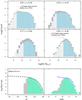 |
Fig. 8 Upper panel: stellar mass distribution of the four redshift bins. The stellar mass histograms for each sample are shown before (dark gray) and after (light gray) the quality control. The stellar mass distributions at the end of the data analysis are compared to the local stellar mass function from Baldry et al. (2012). The light blue histograms show the stellar mass intervals for which the samples are representative. Lower panel: absolute magnitude and stellar mass distribution of SDSS galaxies in the redshift range 0.07 <z< 0.1. The gray histogram corresponds to all the galaxies within the redshift range above the SDSS magnitude limit mr< 17.7. The green histogram corresponds to the distribution of a volume-limited sample in the same redshift range and Mr< −20.62 (Mr limit at z ~ 0.1 for the SDSS). The Mr and stellar mass distributions were compared to the local luminosity function from Loveday et al. (2012; back circle line in right panel) and local stellar mass function from Baldry et al. (2012; blue circle line in left panel), respectively. |
Emission-line galaxies are then spectrally classified according to the presence or absence of certain emission lines as follows: strong-line galaxies (SLG) if [O ii] λ3727, Hβ, [O iii] λ5007, and [N ii] λ6583 are detected over a S/N> 5; or weak-line galaxies (WLG) if at least one of the above lines is undetected (see dashed diagonal area in Fig. 9). We followed the classification of Cid Fernandes et al. (2010, hereafter CF10) where WL-H corresponds to galaxies with all strong lines detected except Hβ, WL-O are galaxies without [O iii] λ5007, WL-O2 are galaxies without [O ii] λ3727, and finally WL-Other for galaxies where two or more lines are undetected (see dashed horizontal area in Fig. 9). The statistics over all samples are given in Table 4. About 92% of galaxies with all four lines detected are in the emission-line galaxy sample (EW(Hα) > 10 Å).
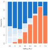 |
Fig. 9 Fraction of star-forming (blue bars) and quiescent galaxies (red bars) in the 0.07 <z< 0.1 sample as a function of the stellar mass. Weak-line galaxies are represented as diagonal dashes and galaxies with fewer than three emission lines detected are shown with horizontal dashes. |
As expected, we observe a decrease of the fraction of emission-line galaxies with increasing stellar mass: for instance, from 62% at log M∗= 9.4 to 24% at log M∗= 10.6 in the z = 0.08 sample. At a given stellar mass, the fraction of emission-line galaxies increases with redshift. For example, the fraction of emission-line log M∗= 10.6 galaxies is 24% at z = 0.08 and 54% at z = 0.27.
Statistics of spectral classes for the four redshift subsamples.
5.3. AGN host
A large number of the diagnostics for determining physical quantities of the ISM are based on the assumption that the gas is exclusively photoionized by massive stars. This excludes the use of these diagnostics for active galactic nuclei (AGN) hosts. In the optical, AGN hosts are classified into three spectral categories: Seyfert I, Seyfert II, and LINERs. We note that QSOs are largely excluded in GAMA by the selection against point-like sources (Baldry et al. 2010). The Seyfert Is are identified during quality control I (Sect. 3.1.2) based on their characteristic broad emission lines.
We used the Baldwin-Phillips-Terlevich (BPT) diagram (Baldwin et al. 1981) that compares the line ratios of [O iii] λλ4959, 5007/Hβ and [N ii] λ6583/Hα to distinguish between star-forming galaxies and AGN. Figure 10a shows the location of the 0.07 <z< 0.1 strong-line galaxies in the BPT parameter space. The line detection threshold is set to (S/N)line> 5. The galaxies fall into two well-defined branches: the left branch populated with star-forming galaxies, and the right branch with high [N ii] λ6583/Hα attributed to AGN-dominated galaxies (Seyfert II and LINERs). We used both the observationally derived separation of Kauffmann et al. (2003a, hereafter K03) and the theoretical limit of Kewley et al. (2006, hereafter K06) to classify galaxies. A galaxy is classified as purely star-forming if its position in the BPT diagram is below the K03 line. This restrictive condition excludes galaxies for which the contribution from AGN to the Hβ line is higher than 3%. In contrast, the highest starburst line from K06 only excludes objects for which the high ionization energy is incompatible with a stellar origin. Above the K06 limit, more than 20−30% of the Hβ flux is produced by AGN radiation. We classified galaxies that lie between the K03 and K06 lines as intermediate. Traditionally, the galaxies in this intermediate region have been classified as composite AGN+star-forming. However, CF10 pointed out that this designation is misleading since a high fraction of the objects falling in this region are potentially quiescent systems devoid of AGN. Using integral field spectroscopy, the results of Singh et al. (2013) have corroborated that a large portion of composite AGN+SF, namely the majority of systems falling in the LINER region, are quiescent systems without AGN activity. In these galaxies, the gas is photoionized by the radiation arising from stars at late stages of their stellar evolution, such as TP-AGB stars. More recently, Sánchez et al. (2015) have shown that the emission from H ii regions is affected by the underlying stellar population. H ii regions located in older systems fall in the bottom right corner of the BTP diagram. Moreover, a non-negligible fraction (~14%) of H ii regions falls in the intermediate region. We therefore kept composite galaxies in our sample of star-forming galaxies, but analyzed them separately from the main star-forming sample. Since the metallicity calibrations are based on line ratios of pure star-forming galaxies, metallicities measured on composite galaxies may not be valid.
Contamination by AGN of weak-line galaxies was also determined using the above scheme (Fig. 10, panel c). The upper limit on the flux is assumed for undetected lines of WL-O and WL-O2 galaxies. As such, the [O iii]/Hβ and [O iii]/[O ii] ratio corresponds to an upper limit for WL-O and the [O iii]/[O ii] are lower limits for WL-O2. For the WL-H, the Hβ flux was substituted with the flux of Hα divided by the theoretical ratio Hα/Hβ ~ 3.0 assuming case B recombination and with a typical electron temperature of around 5000 K. Since the dust extinction was not taken into account, the estimated [O iii]/Hβ of WL-H is a lower limit. The bulk of WL-H are compatible with an ionizing flux produced by LINER-like objets or intermediate-LINERs with average metallicities in agreement with CF10. The location of the WL-O galaxies in the BPT and BPTO2 diagram confirms that this class of galaxies is mainly composed of SF galaxies with high metallicities. WL-O2 are mainly metal-rich star-forming or Seyfert (intermediate and AGN) galaxies. This illustrates the importance of accounting for WL-O and WL-O2 galaxies to avoid selection biases when investigating the statistical properties of star-forming galaxies.
LINERs were distinguished from Seyfert II galaxies by the BPTO2 diagram (see Fig. 10, panel b) in [O ii]/[O iii] versus [N ii] λ6583/Hα. CF10 have shown that this diagram is more effective at separating LINERs from Seyferts because the [O ii]/[O iii] ratio is more sensitive than the [O iii] λλ4959, 5007/Hβ ratio to the ionization state.
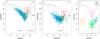 |
Fig. 10 Panel a) BPT diagrams for the 0.07 <z< 0.1 strong-line galaxies. The symbol codes the classification of the targets according to their location in the BPT diagrams: AGN (filled symbols), intermediate (open symbols) and pure star-forming (stars).Targets above the dot-dashed line are AGN/LINER hosts (solid symbols) according to the theoretical separation of Kewley et al. (2006). This separation corresponds to the theoretical limit when assuming only stellar photoionizing radiation. The dashed line corresponds to the empirical limit between star-forming galaxies and AGN/LINERs from Kauffmann et al. (2003a). Galaxies falling between the two lines are composite SF-AGN galaxies. Below the Kauffmann et al. (2003a) line, galaxies are classified as pure star-forming galaxies. The solid line shows the separation between Seyfert and LINERs. The color codes the classification of intermediate and pure AGN into LINERs (green) and Seyferts (red) according to their location on the BPTO2 diagram. Panel b) The BPTO2 diagram for 0.07 <z< 0.1 sample. The symbols are the same as for panel a). This diagnostic diagram has been used to distinguish Seyferts from LINERs for galaxies classified as AGN in the BPT diagram. Panel c) BPT diagrams for the weak-line galaxies in the 0.07 <z< 0.1 sample. The symbols represent the spectral classification of the WLGs with WLG-H as blue crosses, WLG-O as green stars, WLG-O2 as violet circles, and WLG-OH as open red triangles. |
6. Properties of the ISM of star-forming galaxies
6.1. Dust extinction from Balmer decrement
The relative strengths between Balmer recombination lines are nearly constant in the typical range of conditions of H ii regions in galaxies (Osterbrock 1989). The difference between the theoretical and the observed ratio of Balmer lines gives an estimate of the intrinsic extinction. The expected Balmer line ratios are Hα /Hβ = 3.00, Hγ/Hβ = 0.46, and Hγ/Hα = 0.15 (Osterbrock 1989) for case B recombination and H ii regions with a typical electron temperature5 of around 5000 K and electron densities around 104 cm-2. We assume below an average interstellar extinction law with RV = 3.1. The median extinction is AV = 0.89. The uncertainties on the fluxes are propagated into the extinction estimates.
We derived the extinction from three Balmer line ratios: Hα/Hβ, Hγ/Hα, and Hγ/Hβ. In Fig. 11 we show a comparison of the extinction derived from the Hα/Hβ and Hγ/Hα sets of line ratios. The extinction measured using these two ratios agrees within an rms of 0.64. The agreement between the two estimators confirms the quality of the stellar absorption subtraction under the Balmer lines. Only targets with Balmer lines with (S/N)line> 5 are shown. The median extinction given by the Hγ/Hα ratio is slightly higher (AV = 1.07) than that based on Hα/Hβ.
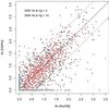 |
Fig. 11 Comparison of extinction estimates based on two Balmer decrements, Hα /Hβ and Hγ/Hα. The two dashed lines represent an rms of ±0.64 mag. |
6.2. SFR from Hα luminosity
We computed the SFR from the luminosity of the Hα line, SFRHα, using the Kennicutt & Evans (2012) calibration. Hα fluxes were corrected for the underlying continuum absorption by the stellar continuum fit described in Sect. 3.2 and were corrected for dust obscuration using the extinction estimated from Balmer decrement. Because Hα lines were measured from the flux calibrated spectra, SFRHα measurements include an implicit correction for fibre aperture effects. The SFRHα is given by ![Mathematical equation: \begin{eqnarray} {\it SFR}_{{\rm H}\alpha} = F_{{\rm H}\alpha} \, 10^{\, 0.4 [ E(B-V) \, \kappa_{{\rm H}\alpha}]} \, D_{\rm L}^2 \times 7.9 \times 10^{-42}, \end{eqnarray}](/articles/aa/full_html/2016/06/aa27836-15/aa27836-15-eq148.png) (2)where FHα is the flux of the Hα line corrected for the underlying stellar absorption (in ergs/s/cm2/Å), DL is the luminosity distance in cm, and κHα the value of the extinction law at the wavelength of Hα.
(2)where FHα is the flux of the Hα line corrected for the underlying stellar absorption (in ergs/s/cm2/Å), DL is the luminosity distance in cm, and κHα the value of the extinction law at the wavelength of Hα.
6.3. Metallicity measurements
In the majority of cases, the metallicity cannot be measured from the direct method based on the electron temperature because the auroral lines (e.g., [O iii] λ4363) are too faint. To overcome this difficulty, empirical calibrations between ratios of strong emission lines and the metallicity were implemented. These strong-line ratios do not directly measure the metallicity of the H ii regions, but they are metallicity sensitive. There is a large number of strong-line ratios in the literature, and the selection of the best method is still debated. In this work, we used the popular strong-emission-line method based on the R23 index: ![Mathematical equation: \begin{equation} R_{23}=\frac{[\mathrm{O\,II}]\lambda \lambda3726,3729 + [\mathrm{O\,III}] \lambda\lambda 4959,5007}{\mathrm{H\beta}}, \end{equation}](/articles/aa/full_html/2016/06/aa27836-15/aa27836-15-eq154.png) (3)with the calibration of Kobulnicky & Kewley (2004) based on photoionization models. The R23 index is double valued with 12 + log(O/H). The selection between the upper and lower branch calibration was made from the O2N2 index defined as [N ii]λ6583/[O ii]λλ3726, 3729. The metallicity conversion is highly uncertain (>1 dex) in the turning zone of the R23 calibration around 12 + log(O/H) ~ 8.20−8.40. The KK04 calibration includes the estimation of the ionization parameter through the [O iii]/[O ii] ratio. This reduces the uncertainties on the metallicity measurements. We followed the equations and methods described in Appendix A of Kewley & Ellison (2008). Metallicity limits were estimated for the WL-H, WL-O, WL-O2, and WL-N galaxies using the flux upper limits for the missing lines. For the WL-H galaxies, the Hβ flux was substituted by the Hα divided by the theoretical ratio Hα /Hβ.
(3)with the calibration of Kobulnicky & Kewley (2004) based on photoionization models. The R23 index is double valued with 12 + log(O/H). The selection between the upper and lower branch calibration was made from the O2N2 index defined as [N ii]λ6583/[O ii]λλ3726, 3729. The metallicity conversion is highly uncertain (>1 dex) in the turning zone of the R23 calibration around 12 + log(O/H) ~ 8.20−8.40. The KK04 calibration includes the estimation of the ionization parameter through the [O iii]/[O ii] ratio. This reduces the uncertainties on the metallicity measurements. We followed the equations and methods described in Appendix A of Kewley & Ellison (2008). Metallicity limits were estimated for the WL-H, WL-O, WL-O2, and WL-N galaxies using the flux upper limits for the missing lines. For the WL-H galaxies, the Hβ flux was substituted by the Hα divided by the theoretical ratio Hα /Hβ.
In contrast with previous GAMA M − Z studies (Foster et al. 2012; Lara-López et al. 2013), we did not use the Pettini & Pagel (2004) calibration based on the O3N2 ratio: O3N2 = log([O iii] λ5007/Hβ)/log([N ii] λ6583/Hα). Although this calibration is insensitive to dust extinction, ratios that include nitrogen lines such as the O3N2 are potentially affected by variations of the N/O abundance ratio (Yang et al. 2008; López-Sánchez et al. 2012). This now appears to be an important source of systematics at high redshift z> 2 (Shapley et al. 2015).
7. Mass-metallicity relation for z ≲ 0.3
In this section, we apply our emission-lines catalogs to investigate the main scaling relation of chemical evolution: the stellar mass versus gas-phase metallicity (M − Z) relation. This relation has been extensively study in the literature in both the local and distant Universe because it enables us to separate the contributions of various processes6 that are important for galaxy evolution (see Foster et al. 2012; Lara-López et al. 2013, for additional background). This relation is affected by numerous sources of systematics that limit our full understanding of galaxy chemical evolution: emission-line measurements (Rodrigues et al. 2008,e.g., spectral resolution, S/N, and flux calibration), sample size, cosmic variance (Moustakas et al. 2011), choice of the metallicity calibration (Kewley & Ellison 2008), AGN rejection criteria (Kewley & Ellison 2008; Moustakas et al. 2011), and line selection effects (Foster et al. 2012; Juneau et al. 2014; Salim et al. 2014). However, the bulk of selection effect studies have qualitatively investigated large samples regardless of the sample representativity. The four representative samples and associated emission-line catalogs allow us to quantify the selection effect on the shape of the M − Z relation and its evolution.
7.1. Mass-metallicity relation at 0.07<z<0.3
Figure 12 presents the M − Z relation in the redshift bin 0.07 <z< 0.1 for pure star-forming galaxies. We were able to constrain the M − Z relation down to stellar masses of log M∗ = 9.4 at redshifts 0.07 <z< 0.1 (top panel). The M − Z relation was fit with a second-order polynomial (red dashed line) and a linear fit (red solid line). The second-order polynonial fit published in Foster et al. (2012) is shown as a black dashed line. The best fit relations are  (4)for the quadratic function, with ρ = 0.448 and σresiduals = 0.16, and
 ![Mathematical equation: \begin{equation} 12+\log{(\mathrm{O/H})} = 6.63 + 0.22 \log{M_*}[M_\sun] \label{eq_linear} \end{equation}](/articles/aa/full_html/2016/06/aa27836-15/aa27836-15-eq161.png) (5)for the linear function, with ρ = 0.439 and σresiduals = 0.16.
(5)for the linear function, with ρ = 0.439 and σresiduals = 0.16.
The observed scatter (σ ~ 0.16 dex) is larger than previously observed by several studies that were based on SDSS data (e.g., Tremonti et al. 2004). From a sample drawn from the SDSS at the same redshift range, Kewley & Ellison (2008) found a mean scatter of σ ~ 0.10 dex using the same metallicity calibration. However, this sample is only representative down to log M∗ = 10.2. Our sample is representative down to lower masses (log M∗ > 9.4), see the discussion in Sect. 5.1 and Fig. 8, right panel. A larger scatter in the M − Z relation at redshifts 0.07 <z< 0.1 for low stellar masses has also been observed by Zahid et al. (2012) using the DEEP2 survey.
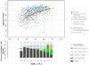 |
Fig. 12 Upper panel: local M − Z relation in the 0.07 <z< 0.1 redshift bin for galaxies classified as pure star-forming galaxies (gray dots) using the KK04 metallicity calibration. The red solid and red dashed line are the linear and second-order polynomial fit to the data, respectively, within the representativity limit of the sample log M∗> 9.4. The blue symbols are galaxies without [O ii] detections (cross) and [O iii] (star). Their metallicities correspond to lower limits estimated from upper limits of the [O ii]λ3727 and [O iii]λ5007 line fluxes. Composite SF-Seyfert and SF-LINERs are represented as green triangles and green cross-squares, respectively. Lower panel: fraction of each spectral type for galaxies verifying the emission-line classification, i.e., EW(Hα) > 10 Å (see Sect. 5.2) in the 0.07 <z< 0.1 sample as a function of the stellar mass. The pure star-forming galaxies shown in the upper panel are represented as a gray area. Composite SF-AGN and AGNs are represented as green and dashed red boxes. Weak-line galaxies, namely galaxies without [O ii]λ3727 and [O iii]λ5007 lines (see Sect. 5.2), are shown in blue. Unclassified galaxies are shown in gray. |
Figure 13 presents the M − Z relation in the four redshift bins for galaxies classified as pure star-forming galaxies. The solid line shows the local M − Z relation derived above. Since sample 0.24 <z< 0.30 is representative down to log M∗> 10.6, the evolution can only be constrained at all redshifts on the last stellar mass bin with a median log M∗= 10.75. At log M∗= 10.6, we observed a decrease of 0.05 dex of metallicity from z = 0.07 to z = 0.3, in agreement with previous SDSS and GAMA work (Lara-López et al. 2009a,b, 2013; Moustakas et al. 2011).
7.2. Quantification of selection effects
Stellar mass versus gas-phase metallicity relations are established for samples of star-forming galaxies. However, the designation “star-forming galaxies” is ambiguous and usually refers to galaxies that have survived selection criteria requiring the simultaneous detection of four or more emission lines needed for AGN host rejection and metallicity estimations. Because the intensity of these lines depends on the properties of galaxies (e.g., extinction and metallicity) this selection may reject specific populations of star-forming galaxies. The addition of these line selection criteria to those from the sample selection leads to a complex combination of selection effects that are difficult to separate. We systematically study each selection criterion used in defining our sample for the M − Z relation. For each criterion, we evaluate its effects on the sample representativity and on the shape of the M − Z relation.
7.2.1. mr selection and color bias
We first investigate the possible selection effects introduced during the definition of the parent sample. Local spectroscopic surveys like SDSS and GAMA are mr-selected. Thus, the parent sample as a whole is subject to the Malmquist bias. To avoid a strong Malmquist bias and possible evolutionary effects, samples are defined in narrow redshift intervals. For instance, local SDSS studies of the M − Z relation commonly define their samples in the 0.05 <z< 0.10 interval (e.g., Kewley & Ellison 2008). As previously demonstrated in Fig. 5.1, these samples are representative only down to log M∗ = 10.2. Below this limit, the sample is potentially affected by color biases.
To evaluate the effect of this color bias on the shape of the M − Z relation, we extracted a subsample of galaxies with mr> 17.77 from the 0.07 <z< 0.10 galaxies to mimic the SDSS selection for the same redshift range. The M∗-color distributions of both samples are shown in the right panel of Fig. 14. The selection on mr approximates a stellar mass selection to first order. But to second order, the mr selection preferentially selects bluer galaxies at masses below the representativity limit (Taylor et al. 2011, see Fig. 6). The effect of the color bias on the M − Z relation is clearly visible in the left panel of Fig. 14, wherein only the bluest galaxies are selected for log M∗< 10.2, missing an important population of red and metal-rich galaxies. The blue population preferentially populates the low metallicity range of the M − Z relation. The red dashed line shows the fit to SDSS-like galaxies alone. The scatter for this relation is σ ~ 0.10 dex, identical to the findings of Kewley & Ellison (2008). Hence, the lower measured scatter found in SDSS-based studies is a consequence of the colour bias and strongly affects the sample below log M∗< 10.2.
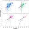 |
Fig. 13 Evolution of the M − Z relation within the GAMA survey from z = 0 to z = 0.3. The four panels show the M − Z relation for the four samples (same color codes as Fig. 1). Sources below and above the stellar mass limit are shown as open and filled symbols, respectively. The solid line shows the best fit to the lowest redshift sample. The samples have also been fitted with a second-order polynomial regardless of the representativity limit. We note that the apparent evolution of the shape of the M − Z relation can be fully explained with this selection effect. |
In addition to lowering the scatter of the M − Z relation, the color bias also artificially steepens the slope of the relation if the representativity limits of the samples are not taken into account. In Fig. 13 we fit the four samples with a quadratic function regardless of the representativity limits (dashed blue line). The slope of the fitted M − Z relation increases with redshift. Conducting an experiment similar to that shown in Fig. 14 on a subsample mimicking the definition of the 0.24 <z< 0.30 sample in terms of Mr results in an identical conclusion: the apparent evolution of the shape of the M − Z relation at redshift z< 0.3 in Fig. 13 (dotted blue line) is fully explained by this color bias, which is a result of the Mr selection. This is the case regardless of the choice of metallicity calibration tested in this work: T04, KK04, M91, and PP04.
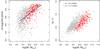 |
Fig. 14 Effect of the mr limit on the shape of the M − Z relation (left panel) and the color-stellar mass sampling (right panel). The gray symbols correspond to all targets in the volume-limited 0.07 <z< 0.1 sample, with a lower Mr limit of Mr = −18.4. The solid black line is the linear fit of the data set above the limit of representativity log M∗= 9.4 given in Eq. (5). We mimic a 0.07 <z< 0.1 sample drawn from SDSS survey by gathering targets with mr< 17.77 from 0.07 <z< 0.1 sample (red symbols). The red dashed line is the quadratic fit to the mr< 17.7 data points. For reference, the fitted M − Z relation on 0.17 <z< 0.24 sample (the best fit shown in the lower left panel of Fig. 13 is plotted as a dotted blue line. |
7.2.2. Simultaneous line detection and AGN host rejection
We defined a representative sample of emission-line galaxies before adding more criteria on simultaneous line detection. This prior selection defined a homogenous sample of emission-line galaxies (or star-forming galaxies) based on a simple criterion: EW(Hα) > 10 Å. This primarily selects star-forming galaxies with morphological types later than Sab. The advantages of selecting emission-line galaxies using a single criterion are the following: (1) it facilitates the task of homogeneously selecting star-forming galaxies at different epochs; (2) selection effects introduced by a single criterion are easier to separate; and (3) selections on Ha EWs are less affected by extinction and metallicity than simultaneous line detection. The purpose of defining an emission-line galaxy sample is to have a reference sample from which it is possible to quantify the fraction of galaxies rejected by simultaneous line detections and AGN host.
Estimating metallicities and rejecting AGN hosts requires the simultaneous detection of various emission lines. Several studies have pointed out that the shape of the M − Z relation depends on the required lines to be detected and their S/N detection threshold (e.g., Foster et al. 2012; Juneau et al. 2014; Salim et al. 2014). As an example, a requirement on the detection of [O iii]λ5007 leads to excluding metal-rich galaxies from the M − Z relation (Foster et al. 2012). The lower panel of Fig. 12 shows the fraction of galaxies with all five lines detected (gray bars), galaxies without the [O iii]λ5007 line (green bars), and galaxies without [O ii]λ3727 (blue bars) over the emission-line galaxy population. At stellar mass log M∗> 10.4, galaxies without [O iii]λ5007 account for up to 20% of the emission-line galaxies. The lower limit on their metallicity estimates indicates that these galaxies have metallicities above 12 + log(O/H) = 9.1 dex on average. The rejection of these galaxies without [O iii] from the M − Z relation may have a potentially strong effect on its shape at high stellar mass.
Another source of systematics at high stellar mass may arise from the selection of star-forming versus AGN host galaxies. About 11% of the emission-line galaxies in our sample were rejected from the M − Z relation because they were classified as LINERs or Seyferts. However, it has been shown by Stasińska et al. (2008, 2015), Singh et al. (2013) that a non-negligible fraction of galaxies classified as LINERs are not AGN hosts, but galaxies harboring old stellar populations. Sánchez et al. (2015) have shown that ionization conditions of H ii regions can be affected by radiation arising from an old underlying stellar population. In our sample, intermediate and pure LINERs account for 6% and 1.2% of emission-line galaxies, respectively. The changes in the ionization conditions prevent us from estimating metallicities in these galaxies using current metallicity calibrations, and therefore we cannot evaluate the effect of this population on the M − Z relation. The selection of star-forming versus AGN host galaxies preferentially rejects massive objects (log M∗> 10.4).
The galaxies rejected by simultaneous line detection criteria or AGN hosts represent 35% of the emission-line galaxies at log M∗ = 10.6. Consequently, the effect of their rejection from the M − Z relation cannot be overlooked. This selection bias particularly affects the high-mass end of the relation. If the properties of these two populations differ from those of the overall population of emission-line systems at high stellar masses, their rejection could explain the apparently reduced scatter compared to low-mass systems (Zahid et al. 2012).
8. Conclusions
We provided a catalog of emission lines for four volume-limited subsamples of GAMA with homogenous measurements for both AAOmega and SDSS spectra. This paper described the data analysis and the performance of our code MARVIN.
The data analysis included a visual quality control of the raw spectra, stellar continuum subtraction, and spectral line measurements. MARVIN automated the main steps of the data analysis, but allowed for interactive inspection. The software controlled the flow of operations in a consistent way by carrying through quality flags for each target at every step and applying appropriate analysis accordingly. Particular care was taken when undetected lines occurred by maintaining a clear record of whether undetected lines were due to instrumental problems (e.g., bad pixels, strong sky lines, and glitches) or were simply weaker than the S/N threshold. The reliability of our algorithm to detect lines is very good with <0.1% failures and <0.04% false detections. The reliability of the measured emission line fluxes translates into a high consistency of measured line ratios such as the [O iii] doublet. We compared our flux measurements with those previously measured using GANDALF (Hopkins et al. 2013). We found good agreement between the two codes at S/N> 10, but significant discrepancies are present in the low S/N regime. About 2.5% of the lines measured by GANDALF are false detections that have failed to pass the MARVIN quality control.
We also derived the main properties of the interstellar medium for star-forming galaxies: dust extinction, AGN-diagnostic, star-formation rate, and metallicity. Dust extinction was estimated using the Balmer decrement from three line ratios. The agreement between the estimators confirms the quality of the stellar absorption correction under the Balmer lines.
We established the stellar mass – metallicity relation in the four intervals of redraft spanned by the samples. At 0.07 <z< 0.1, the observed M − Z relation has a higher scatter at lower stellar mass than previously found in works based on SDSS data. We found that the mass-metallicity relation does not evolve significantly, by less than 0.05 dex, from z = 0.07 to z = 0.34 in the stellar mass range for which the samples are representative (log M∗~ 10.75).
We investigated how selection criteria could distort the representativity of the samples based on which M − Z relation are established. Samples gathered from mr-selected surveys are subject to a color bias at stellar mass below their limit of representativity. Above this limit, the mr cut preferentially selects bluer galaxies. In the same way, redder and more metal-rich galaxies are excluded from the samples at low stellar mass. Failing to take the limits of representativity into account leads to a steeper and tighter M − Z relation. This color selection bias affects all samples selected in r-band (e.g., GAMA and SDSS), even those drawn from volume-limited samples. We highlight the importance of taking the representativity limit of the samples into consideration in term of stellar mass when scaling relations at various redshifts are compared.
The population of pure star-forming galaxies commonly plotted in mass-metallicity relations in the literature and in this work only represents 75% of emission-line galaxies. A significant fraction of emission-line galaxies are excluded from the mass-metallicity relation because metallicity calibrations cannot provide reliable estimates for these objects (e.g., AGN contamination, missing lines, and high metallicities). At stellar masses above log M∗= 10.6, about 65% of the emission-line galaxies are rejected from the mass-metallicity relation. If these rejected targets belong to a population with specific metallicity properties compared to the overall population of emission-line galaxies at the same stellar mass, this could induce strong biases on the shape and dispersion of the mass-metallicity relation in the high-mass range.
nQ indicates the confidence on the spectroscopic redshift assigned to each spectrum, as defined in Liske et al. (2015). Spectra with nQ ≥ 3 have their redshift determined with a confidence level higher than 90%.
We intentionally avoided the luminosity function from Loveday et al. (2012) derived using the GAMA survey to compare our samples with independently determined luminosity functions. The results remain unchanged when using the Loveday et al. (2012) luminosity function.
Absolute magnitudes were extracted from the STARLIGHT database http://www.starlight.ufsc.br
This assumed electron temperature is appropriate for the expected metallicity range of local galaxies, see also the Appendix A in López-Sánchez et al. (2015). Repeating the analysis with 10 000 K does not significantly change our results.
These processes include star formation, outflows powered by supernovae or stellar winds, and infall of gas prompted by mergers or secular accretion.
Acknowledgments
GAMA is a joint European-Australasian project based around a spectroscopic campaign using the Anglo-Australian Telescope. The GAMA input catalog is based on data taken from the Sloan Digital Sky Survey and the UKIRT Infrared Deep Sky Survey. Complementary imaging of the GAMA regions is being obtained by a number of independent survey programs including GALEX MIS, VST KiDS, VISTA VIKING, WISE, Herschel-ATLAS, GMRT, and ASKAP, providing UV to radio coverage. GAMA is funded by the STFC (UK), the ARC (Australia), the AAO, and the participating institutions. The GAMA website is http://www.gama-survey.org/.
References
- Abazajian, K. N., Adelman-McCarthy, J. K., Agüeros, M. A., et al. 2009, ApJS, 182, 543 [NASA ADS] [CrossRef] [Google Scholar]
- Adelman-McCarthy, J. K., Agüeros, M. A., Allam, S. S., et al. 2008, ApJS, 175, 297 [NASA ADS] [CrossRef] [Google Scholar]
- Baldry, I. K., Robotham, A. S. G., Hill, D. T., et al. 2010, MNRAS, 404, 86 [NASA ADS] [Google Scholar]
- Baldry, I. K., Driver, S. P., Loveday, J., et al. 2012, MNRAS, 421, 621 [NASA ADS] [Google Scholar]
- Baldwin, J. A., Phillips, M. M., & Terlevich, R. 1981, PASP, 93, 5 [NASA ADS] [CrossRef] [EDP Sciences] [Google Scholar]
- Bell, E. F., McIntosh, D. H., Katz, N., & Weinberg, M. D. 2003, ApJS, 149, 289 [NASA ADS] [CrossRef] [Google Scholar]
- Brinchmann, J., Charlot, S., White, S. D. M., et al. 2004, MNRAS, 351, 1151 [NASA ADS] [CrossRef] [Google Scholar]
- Brough, S., Hopkins, A. M., Sharp, R. G., et al. 2011, MNRAS, 413, 1236 [NASA ADS] [CrossRef] [Google Scholar]
- Bruzual, G., & Charlot, S. 2003, MNRAS, 344, 1000 [NASA ADS] [CrossRef] [Google Scholar]
- Calzetti, D., Armus, L., Bohlin, R. C., et al. 2000, ApJ, 533, 682 [NASA ADS] [CrossRef] [Google Scholar]
- Cappellari, M., & Emsellem, E. 2004, PASP, 116, 138 [NASA ADS] [CrossRef] [Google Scholar]
- Cardelli, J. A., Clayton, G. C., & Mathis, J. S. 1989, ApJ, 345, 245 [NASA ADS] [CrossRef] [Google Scholar]
- Chabrier, G. 2003, PASP, 115, 763 [NASA ADS] [CrossRef] [Google Scholar]
- Cid Fernandes, R., Mateus, A., Sodré, L., Stasińska, G., & Gomes, J. M. 2005, MNRAS, 358, 363 [NASA ADS] [CrossRef] [Google Scholar]
- Cid Fernandes, R., Stasińska, G., Schlickmann, M. S., et al. 2010, MNRAS, 403, 1036 [NASA ADS] [CrossRef] [Google Scholar]
- Colless, M., Dalton, G., Maddox, S., et al. 2001, MNRAS, 328, 1039 [NASA ADS] [CrossRef] [Google Scholar]
- Driver, S. P., Norberg, P., Baldry, I. K., et al. 2009, Astron. Geophys., 50, 12 [Google Scholar]
- Driver, S. P., Hill, D. T., Kelvin, L. S., et al. 2011, MNRAS, 413, 971 [NASA ADS] [CrossRef] [Google Scholar]
- Foster, C., Hopkins, A. M., Gunawardhana, M., et al. 2012, A&A, 547, A79 [NASA ADS] [CrossRef] [EDP Sciences] [Google Scholar]
- Groves, B., Brinchmann, J., & Walcher, C. J. 2012, MNRAS, 419, 1402 [NASA ADS] [CrossRef] [Google Scholar]
- Hammer, F., Flores, H., Lilly, S. J., et al. 1997, ApJ, 481, 49 [CrossRef] [Google Scholar]
- Hammer, F., Puech, M., Flores, H., & Rodrigues, M. 2016, Studying Distant Galaxies: A Handbook of Methods and Analysis, 1st edn. (World Scientific) [Google Scholar]
- Heavens, A. F., Jimenez, R., & Lahav, O. 2000, MNRAS, 317, 965 [NASA ADS] [CrossRef] [Google Scholar]
- Hill, D. T., Kelvin, L. S., Driver, S. P., et al. 2011, MNRAS, 412, 765 [NASA ADS] [Google Scholar]
- Hopkins, A. M., Driver, S. P., Brough, S., et al. 2013, MNRAS, 430, 2047 [NASA ADS] [CrossRef] [Google Scholar]
- Jones, D. H., Read, M. A., Saunders, W., et al. 2009, MNRAS, 399, 683 [NASA ADS] [CrossRef] [Google Scholar]
- Juneau, S., Bournaud, F., Charlot, S., et al. 2014, ApJ, 788, 88 [NASA ADS] [CrossRef] [Google Scholar]
- Kauffmann, G., Heckman, T. M., Tremonti, C., et al. 2003a, MNRAS, 346, 1055 [Google Scholar]
- Kauffmann, G., Heckman, T. M., White, S. D. M., et al. 2003b, MNRAS, 341, 54 [Google Scholar]
- Kennicutt, Jr., R. C. 1992, ApJ, 388, 310 [NASA ADS] [CrossRef] [Google Scholar]
- Kennicutt, R. C., & Evans, N. J. 2012, ARA&A, 50, 531 [NASA ADS] [CrossRef] [Google Scholar]
- Kennicutt, Jr., R. C., Tamblyn, P., & Congdon, C. E. 1994, ApJ, 435, 22 [Google Scholar]
- Kewley, L. J., & Ellison, S. L. 2008, ApJ, 681, 1183 [NASA ADS] [CrossRef] [Google Scholar]
- Kewley, L. J., Groves, B., Kauffmann, G., & Heckman, T. 2006, MNRAS, 372, 961 [NASA ADS] [CrossRef] [Google Scholar]
- Kobulnicky, H. A., & Kewley, L. J. 2004, ApJ, 617, 240 [NASA ADS] [CrossRef] [Google Scholar]
- Koleva, M., Prugniel, P., Bouchard, A., & Wu, Y. 2009, A&A, 501, 1269 [NASA ADS] [CrossRef] [EDP Sciences] [Google Scholar]
- Lamareille, F., Contini, T., Le Borgne, J., et al. 2006, A&A, 448, 893 [NASA ADS] [CrossRef] [EDP Sciences] [Google Scholar]
- Lara-López, M. A., Cepa, J., Bongiovanni, A., et al. 2009a, A&A, 493, L5 [NASA ADS] [CrossRef] [EDP Sciences] [Google Scholar]
- Lara-López, M. A., Cepa, J., Bongiovanni, A., et al. 2009b, A&A, 505, 529 [NASA ADS] [CrossRef] [EDP Sciences] [Google Scholar]
- Lara-López, M. A., Hopkins, A. M., López-Sánchez, A. R., et al. 2013, MNRAS, 434, 451 [NASA ADS] [CrossRef] [Google Scholar]
- Le Borgne, J., Bruzual, G., Pelló, R., et al. 2003, A&A, 402, 433 [NASA ADS] [CrossRef] [EDP Sciences] [Google Scholar]
- Liang, Y. C., Hammer, F., Flores, H., et al. 2004, A&A, 423, 867 [NASA ADS] [CrossRef] [EDP Sciences] [Google Scholar]
- Liske, J., Baldry, I. K., Driver, S. P., et al. 2015, MNRAS, 452, 2087 [NASA ADS] [CrossRef] [Google Scholar]
- López-Sánchez, Á. R., Dopita, M. A., Kewley, L. J., et al. 2012, MNRAS, 426, 2630 [NASA ADS] [CrossRef] [Google Scholar]
- López-Sánchez, Á. R., Westmeier, T., Esteban, C., & Koribalski, B. S. 2015, MNRAS, 450, 3381 [NASA ADS] [CrossRef] [Google Scholar]
- Loveday, J., Norberg, P., Baldry, I. K., et al. 2012, MNRAS, 420, 1239 [NASA ADS] [CrossRef] [Google Scholar]
- Maraston, C., & Strömbäck, G. 2011, MNRAS, 418, 2785 [NASA ADS] [CrossRef] [Google Scholar]
- Montero-Dorta, A. D., & Prada, F. 2009, MNRAS, 399, 1106 [NASA ADS] [CrossRef] [Google Scholar]
- Moustakas, J., & Kennicutt, Jr., R. C. 2006, ApJS, 164, 81 [NASA ADS] [CrossRef] [Google Scholar]
- Moustakas, J., Zaritsky, D., Brown, M., et al. 2011, ArXiv e-prints [arXiv:1112.3300] [Google Scholar]
- Ocvirk, P., Pichon, C., Lançon, A., & Thiébaut, E. 2006, MNRAS, 365, 46 [NASA ADS] [CrossRef] [Google Scholar]
- Oh, K., Sarzi, M., Schawinski, K., & Yi, S. K. 2011, ApJS, 195, 13 [NASA ADS] [CrossRef] [Google Scholar]
- Osterbrock, D. E. 1989, Astrophysics of gaseous nebulae and active galactic nuclei (University Science Books) [Google Scholar]
- Pettini, M., & Pagel, B. E. J. 2004, MNRAS, 348, L59 [NASA ADS] [CrossRef] [Google Scholar]
- Rodrigues, M., Hammer, F., Flores, H., et al. 2008, A&A, 492, 371 [NASA ADS] [CrossRef] [EDP Sciences] [Google Scholar]
- Rola, C., & Pelat, D. 1994, A&A, 287, 676 [NASA ADS] [Google Scholar]
- Salim, S., Rich, R. M., Charlot, S., et al. 2007, ApJS, 173, 267 [NASA ADS] [CrossRef] [Google Scholar]
- Salim, S., Lee, J. C., Ly, C., et al. 2014, ApJ, 797, 126 [NASA ADS] [CrossRef] [Google Scholar]
- Salpeter, E. E. 1955, ApJ, 121, 161 [Google Scholar]
- Sánchez, S. F., Pérez, E., Rosales-Ortega, F. F., et al. 2015, A&A, 574, A47 [NASA ADS] [CrossRef] [EDP Sciences] [Google Scholar]
- Saulder, C., Mieske, S., Zeilinger, W. W., & Chilingarian, I. 2013, A&A, 557, A21 [NASA ADS] [CrossRef] [EDP Sciences] [Google Scholar]
- Saunders, W., Bridges, T., Gillingham, P., et al. 2004, in Ground-based Instrumentation for Astronomy, eds. A. F. M. Moorwood, & M. Iye, SPIE Conf. Ser., 5492, 389 [Google Scholar]
- Schlegel, D. J., Finkbeiner, D. P., & Davis, M. 1998, ApJ, 500, 525 [NASA ADS] [CrossRef] [Google Scholar]
- Shapley, A. E., Reddy, N. A., Kriek, M., et al. 2015, ApJ, 801, 88 [NASA ADS] [CrossRef] [Google Scholar]
- Sharp, R., Saunders, W., Smith, G., et al. 2006, in SPIE Conf. Ser., 6269 [Google Scholar]
- Singh, R., van de Ven, G., Jahnke, K., et al. 2013, A&A, 558, A43 [NASA ADS] [CrossRef] [EDP Sciences] [Google Scholar]
- Smith, G., Brzeski, J., Miziarski, S., et al. 2004, in Astronomical Structures and Mechanisms Technology, eds. J. Antebi, & D. Lemke, SPIE Conf. Ser., 5495, 348 [Google Scholar]
- Stasińska, G., Vale Asari, N., Cid Fernandes, R., et al. 2008, MNRAS, 391, L29 [NASA ADS] [Google Scholar]
- Stasińska, G., Costa-Duarte, M. V., Vale Asari, N., CidFernandes, R., & Sodré, L. 2015, MNRAS, 449, 559 [NASA ADS] [CrossRef] [Google Scholar]
- Storey, P. J., & Zeippen, C. J. 2000, MNRAS, 312, 813 [Google Scholar]
- Sutherland, W., Emerson, J., Dalton, G., et al. 2015, A&A, 575, A25 [NASA ADS] [CrossRef] [EDP Sciences] [Google Scholar]
- Taylor, E. N., Hopkins, A. M., Baldry, I. K., et al. 2011, MNRAS, 418, 1587 [NASA ADS] [CrossRef] [Google Scholar]
- Taylor, E. N., Hopkins, A. M., Baldry, I. K., et al. 2015, MNRAS, 446, 2144 [NASA ADS] [CrossRef] [Google Scholar]
- Tojeiro, R., Heavens, A. F., Jimenez, R., & Panter, B. 2007, MNRAS, 381, 1252 [NASA ADS] [CrossRef] [Google Scholar]
- Tremonti, C. A., Heckman, T. M., Kauffmann, G., et al. 2004, ApJ, 613, 898 [NASA ADS] [CrossRef] [Google Scholar]
- Wall, J. V., & Jenkins, C. R. 2012, Practical Statistics for Astronomers (Cambridge University Press) [Google Scholar]
- Yang, Y., Flores, H., Hammer, F., et al. 2008, A&A, 477, 789 [NASA ADS] [CrossRef] [EDP Sciences] [Google Scholar]
- Zahid, H. J., Bresolin, F., Kewley, L. J., Coil, A. L., & Davé, R. 2012, ApJ, 750, 120 [NASA ADS] [CrossRef] [Google Scholar]
All Tables
All Figures
|
Fig. 1 Redshift versus Petrosian r-band absolute magnitude (Mr) for GAMA sources with reliable redshift and stellar mass estimates (gray dots). The four color boxes correspond to each of the stellar-mass-selected samples: 0.07 <z< 0.1 (blue), 0.1 <z< 0.15 (green), 0.17 <z< 0.2 (pink), and 0.2<z<0.3 (red), and are representative between −23 <Mr< − 18.4, −23 <Mr< − 19.2, −23 <Mr< − 20.4, and −23 <Mr< − 21, respectively. The dashed and dotted lines are the Mr limits corresponding to the apparent magnitude limits of the SDSS (mr> 14.5 for the bright limit and mr< 17.7). The black solid line indicates Mr limits corresponding to the apparent magnitude limits of GAMA (mr< 19.8). |
| In the text | |
|
Fig. 2 Assessment of the spectrophotometric accuracy of the GAMA spectra. The flux-calibrated spectra (light gray line) are compared with the multiband photometry from SDSS (open red squares). The solid black line corresponds to a heavy smoothing of the spectrum, and the solid circles are the summed fluxes from the spectrum. Since the flux calibration is more problematic at the edges of the spectra, we have estimated two intermediate pseudo-bands ug and iz, in the AB system (λc = 4118 Å; 8206 Å), to be used as visual guidelines. We assume that the SED is roughly linear between the u and b-bands and between the i and z-bands. The fluxes in these two intermediate bands are estimated in the spectra by taking the median value around a small region of the central wavelength. |
| In the text | |
|
Fig. 3 Example spectra representing our four quality flags. Panel A) shows an example of a fringed spectrum. A spectrum with failed spectrophotometry is shown in panel B), wherein the red open squares are the fluxes estimated from the SDSS photometry inside the fibre aperture. Panel C) shows a spectrum with clear splicing problems around observed frame 5700 Å, where the blue and red spectra have been unsuccessfully joined. An example spectrum with broad hydrogen emission lines classified as Seyfert I is shown in panel D). |
| In the text | |
|
Fig. 4 Typical accuracy of the stellar continuum subtraction. Top panel: raw (gray), after correcting the low-frequency residuals (black) and synthetic spectra for a typical sample target. The correction of the low-frequency residuals are typically <5%. In this spectrum the correction is hardly visible. The correction is visible around 7000 Å, corresponding to a region typically affected by sky subtraction residuals. Lower panel: residuals after subtracting the synthetic spectrum. |
| In the text | |
|
Fig. 5 Fitted emission lines for target G15-Y3-001-058 (also shown in Fig. 4). The input spectrum is shown as a black solid line. The red solid lines show the best fit to the emission lines and the green line corresponds to the weight given to pixels based on the flux uncertainties. Bad pixels and regions affected by strong sky lines have been rejected during the fit. Fitted lines with (S/N)line< 5 are rejected. |
| In the text | |
|
Fig. 6 Distribution of observed ratio of [O iii] λ4959/[O iii] λ5007 in 0.10 <z< 0.15 sample for S/Nline> 7. The solid arrow corresponds to the theoretical ratio of 1/2.98 (Storey & Zeippen 2000). The median and the 68th percentiles are represented as the dashed and dotted red lines, respectively. The median flux ratio is 0.333 with a standard deviation of 0.07, within 1 per cent of the theoretical value. |
| In the text | |
|
Fig. 7 Comparison between the flux measured by MARVIN and GANDALF for the spectra in sample 0.1 <z< 0.15. Only lines detected above a S/N threshold of 7 by both codes have been selected. Below this S/N threshold the fluxes are systematically overestimated, see discussion in the text. The false detections have been excluded in the comparison.The dashed and dotted lines are the median and standard deviation of the distributions, respectively. |
| In the text | |
|
Fig. 8 Upper panel: stellar mass distribution of the four redshift bins. The stellar mass histograms for each sample are shown before (dark gray) and after (light gray) the quality control. The stellar mass distributions at the end of the data analysis are compared to the local stellar mass function from Baldry et al. (2012). The light blue histograms show the stellar mass intervals for which the samples are representative. Lower panel: absolute magnitude and stellar mass distribution of SDSS galaxies in the redshift range 0.07 <z< 0.1. The gray histogram corresponds to all the galaxies within the redshift range above the SDSS magnitude limit mr< 17.7. The green histogram corresponds to the distribution of a volume-limited sample in the same redshift range and Mr< −20.62 (Mr limit at z ~ 0.1 for the SDSS). The Mr and stellar mass distributions were compared to the local luminosity function from Loveday et al. (2012; back circle line in right panel) and local stellar mass function from Baldry et al. (2012; blue circle line in left panel), respectively. |
| In the text | |
|
Fig. 9 Fraction of star-forming (blue bars) and quiescent galaxies (red bars) in the 0.07 <z< 0.1 sample as a function of the stellar mass. Weak-line galaxies are represented as diagonal dashes and galaxies with fewer than three emission lines detected are shown with horizontal dashes. |
| In the text | |
|
Fig. 10 Panel a) BPT diagrams for the 0.07 <z< 0.1 strong-line galaxies. The symbol codes the classification of the targets according to their location in the BPT diagrams: AGN (filled symbols), intermediate (open symbols) and pure star-forming (stars).Targets above the dot-dashed line are AGN/LINER hosts (solid symbols) according to the theoretical separation of Kewley et al. (2006). This separation corresponds to the theoretical limit when assuming only stellar photoionizing radiation. The dashed line corresponds to the empirical limit between star-forming galaxies and AGN/LINERs from Kauffmann et al. (2003a). Galaxies falling between the two lines are composite SF-AGN galaxies. Below the Kauffmann et al. (2003a) line, galaxies are classified as pure star-forming galaxies. The solid line shows the separation between Seyfert and LINERs. The color codes the classification of intermediate and pure AGN into LINERs (green) and Seyferts (red) according to their location on the BPTO2 diagram. Panel b) The BPTO2 diagram for 0.07 <z< 0.1 sample. The symbols are the same as for panel a). This diagnostic diagram has been used to distinguish Seyferts from LINERs for galaxies classified as AGN in the BPT diagram. Panel c) BPT diagrams for the weak-line galaxies in the 0.07 <z< 0.1 sample. The symbols represent the spectral classification of the WLGs with WLG-H as blue crosses, WLG-O as green stars, WLG-O2 as violet circles, and WLG-OH as open red triangles. |
| In the text | |
|
Fig. 11 Comparison of extinction estimates based on two Balmer decrements, Hα /Hβ and Hγ/Hα. The two dashed lines represent an rms of ±0.64 mag. |
| In the text | |
|
Fig. 12 Upper panel: local M − Z relation in the 0.07 <z< 0.1 redshift bin for galaxies classified as pure star-forming galaxies (gray dots) using the KK04 metallicity calibration. The red solid and red dashed line are the linear and second-order polynomial fit to the data, respectively, within the representativity limit of the sample log M∗> 9.4. The blue symbols are galaxies without [O ii] detections (cross) and [O iii] (star). Their metallicities correspond to lower limits estimated from upper limits of the [O ii]λ3727 and [O iii]λ5007 line fluxes. Composite SF-Seyfert and SF-LINERs are represented as green triangles and green cross-squares, respectively. Lower panel: fraction of each spectral type for galaxies verifying the emission-line classification, i.e., EW(Hα) > 10 Å (see Sect. 5.2) in the 0.07 <z< 0.1 sample as a function of the stellar mass. The pure star-forming galaxies shown in the upper panel are represented as a gray area. Composite SF-AGN and AGNs are represented as green and dashed red boxes. Weak-line galaxies, namely galaxies without [O ii]λ3727 and [O iii]λ5007 lines (see Sect. 5.2), are shown in blue. Unclassified galaxies are shown in gray. |
| In the text | |
|
Fig. 13 Evolution of the M − Z relation within the GAMA survey from z = 0 to z = 0.3. The four panels show the M − Z relation for the four samples (same color codes as Fig. 1). Sources below and above the stellar mass limit are shown as open and filled symbols, respectively. The solid line shows the best fit to the lowest redshift sample. The samples have also been fitted with a second-order polynomial regardless of the representativity limit. We note that the apparent evolution of the shape of the M − Z relation can be fully explained with this selection effect. |
| In the text | |
|
Fig. 14 Effect of the mr limit on the shape of the M − Z relation (left panel) and the color-stellar mass sampling (right panel). The gray symbols correspond to all targets in the volume-limited 0.07 <z< 0.1 sample, with a lower Mr limit of Mr = −18.4. The solid black line is the linear fit of the data set above the limit of representativity log M∗= 9.4 given in Eq. (5). We mimic a 0.07 <z< 0.1 sample drawn from SDSS survey by gathering targets with mr< 17.77 from 0.07 <z< 0.1 sample (red symbols). The red dashed line is the quadratic fit to the mr< 17.7 data points. For reference, the fitted M − Z relation on 0.17 <z< 0.24 sample (the best fit shown in the lower left panel of Fig. 13 is plotted as a dotted blue line. |
| In the text | |
Current usage metrics show cumulative count of Article Views (full-text article views including HTML views, PDF and ePub downloads, according to the available data) and Abstracts Views on Vision4Press platform.
Data correspond to usage on the plateform after 2015. The current usage metrics is available 48-96 hours after online publication and is updated daily on week days.
Initial download of the metrics may take a while.