| Issue |
A&A
Volume 590, June 2016
|
|
|---|---|---|
| Article Number | A126 | |
| Number of page(s) | 16 | |
| Section | Cosmology (including clusters of galaxies) | |
| DOI | https://doi.org/10.1051/0004-6361/201527630 | |
| Published online | 27 May 2016 | |
The relation between mass and concentration in X-ray galaxy clusters at high redshift
1
Dipartimento di Fisica e Astronomia, Università di
Bologna, viale Berti Pichat
6/2, 40127
Bologna,
Italy
e-mail:
stefania.amodeo@obspm.fr
2
INAF, Osservatorio Astronomico di Bologna, via Ranzani 1,
40127
Bologna,
Italy
3
INFN, Sezione di Bologna, viale Berti Pichat 6/2,
40127
Bologna,
Italy
4
Faculty of Physics, Ludwig-Maximilians-Universitaet,
Scheinerstr. 1,
81679
Muenchen,
Germany
5
Excellence Cluster Universe, Boltzmannstr. 2, 85748
Garching,
Germany
Received: 23 October 2015
Accepted: 5 April 2016
Context. Galaxy clusters are the most recent, gravitationally bound products of the hierarchical mass accretion over cosmological scales. How the mass is concentrated is predicted to correlate with the total mass in the halo of the cluster, wherein systems at higher mass are less concentrated at given redshift and, for any given mass, systems with lower concentration are found at higher redshifts.
Aims. Through a spatial and spectral X-ray analysis, we reconstruct the total mass profile of 47 galaxy clusters observed with Chandra in the redshift range 0.4 <z< 1.2, which we selected to exclude major mergers, to investigate the relation between the mass and dark matter concentration and the evolution of this relation with redshift. This sample is the largest investigated so far at z> 0.4, and is well suited to providing the first constraint on the concentration–mass relation at z> 0.7 from X-ray analysis.
Methods. Under the assumption that the distribution of the X-ray emitting gas is spherically symmetric and in the hydrostatic equilibrium with the underlined gravitational potential, we combine the deprojected gas density and spectral temperature profiles through the hydrostatic equilibrium equation to recover the parameters that describe a Navarro-Frenk-White total mass distribution. The comparison with results from weak-lensing analysis reveals a very good agreement both for masses and concentrations. The uncertainties are however too large to make any robust conclusion about the hydrostatic bias of these systems.
Results. The distribution of concentrations is well approximated by a log-normal function in all the mass and redshift ranges investigated. The relation is well described by the form c ∝ MB(1 + z)C with B = −0.50 ± 0.20, C = 0.12 ± 0.61 (at 68.3% confidence). This relation is slightly steeper than that predicted by numerical simulations (B ~ −0.1) and does not show any evident redshift evolution. We obtain the first constraints on the properties of the concentration–mass relation at z> 0.7 from X-ray data, showing a reasonable good agreement with recent numerical predictions.
Key words: galaxies: clusters: general / intergalactic medium / X-rays: galaxies / cosmology: observations / dark matter
© ESO, 2016
1. Introduction
Within the standard cosmological model, structure formation takes place from the gravitational collapse of small perturbations in a quasi-homogeneus Universe dominated by cold dark matter (CDM). The collapse proceeds from smaller to larger scales giving rise to a hierarchical clustering of cosmic structures. In this framework, galaxy clusters, as they are the largest nearly virialised collapsed objects in the observable Universe, are also the last to form. Therefore, they are fundamental tools for understanding the formation and evolution of cosmic structures.
Numerical N-body simulations predict that dark matter halos have a universal density profile characterised by two parameters: the scale radius rs, defined as the radius at which the logarithmic density slope is −2, and the concentration c, defined as the ratio between R2001 and rs (Navarro et al. 1997, hereafter NFW). Because of the hierarchical nature of structure formation (low-mass objects form earlier than high-mass objects) and the fact that collapsed objects retain information on the background density at the time of their formation (the background average matter density was higher in the past), concentration and mass are related so that systems with higher masses are less concentrated and, at a given mass, lower concentrations are expected at higher redshifts (e.g. Muñoz-Cuartas et al. 2011). Moreover, the properties of the background Universe depend on the set of cosmological parameters adopted. Models with lower matter density and lower normalisation of the linear power spectrum result in a later assembly redshift, so less concentrated halos are expected at a given mass. Therefore, the c(M,z) relation contains a wealth of cosmological information. Several works have been performed to characterise this relation, both numerically and observationally, but there are tensions between them. Numerical simulations by Dolag et al. (2004), Duffy et al. (2008), Bhattacharya et al. (2013), De Boni et al. (2013), Ludlow et al. (2014), and Dutton & Macciò (2014) indicate that concentration and mass are anti-correlated for all the mass ranges and redshifts investigated with a mass dependence that is slightly reduced at larger redshift. Observations of galaxy clusters at low redshift confirm the expected anti-correlation between c and M, but they generally find a steeper slope and a higher normalisation compared to the theoretical relation (Buote et al. 2007; Schmidt & Allen 2007; Ettori et al. 2010; Merten et al. 2015). Whether this discrepancy is due to observational selection biases (e.g. Meneghetti et al. 2014; Sereno et al. 2015) or to the lack of some fundamental physics in numerical models is still an open question. Both simulations (e.g. De Boni et al. 2013) and observations (Ettori et al. 2010) agree about the influence of the dynamical state of a cluster on its concentration; that is, more relaxed systems are more concentrated at a fixed mass. A different trend emerges from simulations by Prada et al. (2012) and Klypin et al. (2014). They predict that at high redshifts the c(M) relation has a plateau and an upturn at the typical masses of galaxy clusters. However, as shown in Ludlow et al. (2012; see also Correa et al. 2015), the plateau and the upturn disappear when the relaxed halos are the only ones considered. Properties of observed mass-concentration relations are strongly sample dependent (Sereno et al. 2015). The predicted slope in signal-selected samples can be much steeper than that of the underlying population characterising dark matter-only clusters. Over-concentrated clusters can be preferentially included and this effect is more prominent at the low-mass end. Sereno et al. (2015) found this trend both in the X-ray selected samples Cluster Lensing And Supernova survey with Hubble (CLASH; Postman et al. 2012) and Local Cluster Substructure Survey (LOCUSS; Okabe et al. 2010) and in the lensing selected sample Sloan Giant Arcs Survey (SGAS; Hennawi et al. 2008). Statistical and selection biases in observed relations are then to be carefully considered when compared with predictions of the ΛCDM model (Meneghetti et al. 2014). Among the methods used to characterise the c(M) relation, X-ray observations are found to be rather successful since galaxy clusters have a well-resolved, extended emission with a total luminosity that is proportional to the square of the gas density.
In this work, we perform spatial and spectral analysis for a sample of 47 galaxy clusters observed with Chandra in the redshift range 0.4 <z< 1.2, which we selected to exclude major mergers with the aim to (1) reconstruct their total mass profile by assuming a spherical symmetry for the intracluster medium (ICM) distribution and hydrostatic equilibrium between the ICM and the gravitational potential of each cluster; and (2) investigate the relation between their mass and concentration and its evolution with redshift. We consider the largest sample investigated so far at z> 0.4 with the additional purpose of probing the c(M) relation at z> 0.7 for the first time using X-ray data.
The paper is organised as follows: in Sect. 2, we present the sample of Chandra observations selected for the analysis; in Sects. 3 and 4, we describe the data analysis and the method used to reconstruct the clusters mass profiles, respectively; in Sect. 5, we investigate our c(M,z) relation and its redshift evolution. We discuss the properties of the sample and its representativeness in Sect. 6 and we draw our conclusions in Sect. 7. We assume a flat ΛCDM cosmology with Ωm = 0.3, ΩΛ = 0.7, H0 = 70 km s-1 Mpc-1 and  . All quoted errors are 68.3% (1σ) confidence level, unless otherwise stated.
2. The dataset
We retrieved all observations of galaxy clusters with redshift z ≥ 0.4 available at 2 March 2014 from the Chandra public archive. We excluded those galaxy clusters with exposure time shorter than 20 ks in order to have sufficient X-ray count statistics, in particular, for spectral analysis. We also excluded galaxy clusters that to a visual inspection showed evidence of dynamic activity (e.g. presence of major substructures). This restriction minimises the systematic scatter in the mass estimate, since the higher the degree of regular morphology in the X-ray image, the more the cluster is expected to be dynamical relaxed and the more robust is the assumption of the hydrostatic equilibrium of the ICM in the cluster potential well (e.g. Rasia et al. 2006; Poole et al. 2006; Mahdavi et al. 2013; Nelson et al. 2014). Another selection criterion is related to the choice of adopting a NFW as functional form of the cluster gravitational profile, which has two free parameters (scale radius rs and concentration c). Considering that our procedure to reconstruct the mass profile requires independent spectral measurements of the gas temperatures (see Sect. 4), we need a number of independent radial bins that is larger than the number of mass modelling parameters (=2). Therefore, we used only the targets for which we could measure the temperature in at least three independent bins. The final sample is then composed of 47 galaxy clusters spanning a redshift range 0.4 <z< 1.2, as listed in Table 1.
Sample of the galaxy clusters analysed in this work.
The acquired data are reduced using the CIAO 4.7 software (Chandra Interactive Analysis of Observations, Fruscione et al. 2006) and the calibration database CALDB 4.6.5 (December 2014 release2). This procedure includes a filter for the good time intervals associated with each observation and a correction for the charge transfer inefficiency. It removes photons detected in bad CCD columns and pixels, it computes calibrated photon energies by applying ACIS gain maps and it corrects for their time dependence. Moreover, it examines the background light curves during each observation to detect and remove flaring episodes. We identify bright point sources using the wavdetect alogorithm by Vikhlinin et al. (1998), check the results by visual inspection, mask all the detected point sources and exclude them from the following analysis.
3. Spatial and spectral analysis
Obtaining good brightness and temperature profiles is crucial for the quality of the mass estimates. This strongly depends on the quantity and quality of data obtained for each observation, namely the number of counts measured for the observed target and the fraction of counts on the background.
We extract surface brightness radial profiles from the images in the [ 0.7−2 ] keV band by constructing a set of circular annuli around the X-ray emission peak, each one containing at least 100 net source counts. The background counts are estimated from local regions of the same exposure that are free from source emissions (on the same chip as the source region or on another chip of the same type used in the observation). Following this criterion, we manually select from two to four background regions for each cluster. The surface brightness profile is then extracted over an area where the signal-to-noise ratio is always larger than 2, up to the radius  . In Table 1, we quote the number of counts measured for each target in the [ 0.7−2 ] keV band, the number of radial bins obtained to sample the surface brightness profile, and .
For the spectral analysis, we use the CIAO specextract tool to extract the source and background spectra and to construct the redistribution matrix files (RMF) and the ancillary response files (ARF) for each annulus. The RMF associates the appropriate photon energy with each instrument channel, while the ARF includes information on the effective area, the efficiency of the instrument in revealing photons, and any additional energy-dependent efficiencies. The background spectra are extracted from the same background regions used for the spatial analysis. The source spectra are extracted from at least three concentric annuli centred on the X-ray surface brightness centroid up to the radius  where the signal-to-noise is larger than 0.3 in the [ 0.6−7 ] keV band. Each spectrum contains at least 500 net source counts in the [ 0.6−7 ] keV band. For five objects (CL0848.6+4453, LCDCS954, CLJ1113.1-2615, CLJ2302.8+0844, and RDCS1252-2927), we consider a minimum of 200 net counts to resolve the temperature profile in three independent radial bins. In Table 1, we also report the radial limit probed in the spectral analysis () and the number of bins with which we can sample the temperature profiles by integrating the spectra between 0.6 and 7 keV.
For each annulus, the spectrum is analysed with the X-ray spectral fitting software XSPEC (Arnaud 1996). We adopt a collisionally ionised diffuse gas emission model (apec) multiplied by an absorption component (tbabs). In this model, we fix the redshift to the value obtained from the optical spectroscopy and the absorbing equivalent hydrogen column density NH to the value of the Galactic absorption inferred from radio HI maps in Dickey & Lockman (1990). Then, the free parameters in the spectral fitting model are the emission-weighted temperature, metallicity, and normalisation of the thermal spectrum. The fit is performed in the energy range [ 0.6−7 ] keV applying Cash statistics (Cash 1979) as implemented in XSPEC. Cash statistics is a maximum-likelihood estimator based on the Poisson distribution of the detected source plus background counts and is preferable for low signal-to-noise spectra (e.g. Nousek & Shue 1989).
The gas density profile is then obtained through the geometrical deprojection (e.g. Fabian et al. 1981; Ettori et al. 2002) of both the surface brightness profile Sb and the normalisation K of the thermal model fitted in the spectral analysis.
4. The hydrostatic mass profile
The total mass of X-ray luminous galaxy clusters can be estimated from the observed gas density ngas and temperature Tgas profiles. The Euler equation for a spherically symmetric distribution of gas with pressure Pgas and density ρgas, in hydrostatic equilibrium with the underlying gravitational potential φ, requires (Binney & Tremaine 1987) 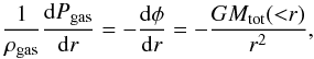 (1)which is better known as the hydrostatic equilibrium equation (HEE). Solving Eq. (1) for the total mass Mtot and considering the perfect gas law, Pgas = ρgaskTgas/ (μmp) = ngaskTgas, we can obtain the total mass of the clusters as a function of our observables, gas density and temperature profiles (see e.g. Ettori et al. 2013, for a recent review),
 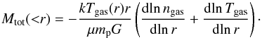 (2)Here, G is the gravitational constant, k is the Boltzmann’s constant, mp is the proton mass, μ = 0.6 is the mean molecular weight of the gas, and ngas = ρgas/μmp is the sum of the electron and ion densities.
We consider a galaxy cluster to be a spherical region with a radius RΔ, where Δ is the mean over-density with respect to the critical density of the Universe at the redshift of the cluster. We define all the quantities describing the mass profile of the cluster in relation to the over-density Δ = 200. We define the masses with respect to the critical density of the Universe. Diemer & Kravtsov (2015) pointed out that the time evolution of the concentration with the peak height ν exhibits the smallest deviations from universality if this definition is adopted.
As described in Ettori et al. (2013), Eq. (2) can be solved at least with two different approaches, adopting either a backwards method or a forwards method.
The backwards method follows the approach described in Ettori et al. (2010). Briefly, it consists in adopting a functional form to describe the total mass profile, while there is no parametrisation of the gas temperature and density profiles. We adopt the NFW profile, so that  (3)where x = r/rs. This model is a function of two parameters: the scale radius rs and concentration c, which are related by the relation R200 = c200 × rs. The best-fit parameters are searched over a grid of values in the (rs,c) plane and they are constrained by minimising the following χ2 statistics:
 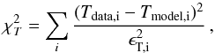 (4)where the sum is performed over the annuli of the spectral analysis; Tdata are the temperature measurements obtained in the spectral analysis; Tmodel are the values obtained by projecting the estimates of Tgas (recovered from the inversion of the HEE Eq. (2) for a given gas density and total mass profiles) over the annuli used in the spectral analysis, according to Mazzotta et al. (2004); and ϵT is the error on the spectral measurements. The search for the minimum in the
  distribution proceeds, first, in identifying a minimum over a grid of 50 × 50 points in which the range of the two free parameters (50 kpc
 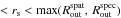 ; 0.2 <c< 20) is divided regularly. Then, we obtain the refined best-fit values for the (rs,c) parameters, looking for a minimum over a 100 × 100 grid in a 5σ range around the first identified minimum. Considering the strong correlation present between the free parameters and to fully represent their probability distribution, we estimate and quote the probability weighted means of the concentration c200 and of the mass M200 in Table 2. The mass is obtained as
  , where R200 = rs × c200 and propagates the joint probability distribution evaluated for the grid of values of the (rs,c) parameters. In Table 2, we quote the best-fit results for c200 and M200 derived from the backwards method.
Results of the mass reconstruction.
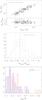 |
Fig. 1 Top: comparison between mass estimates obtained following the forwards method (Mfor) and backwards method (Mback) for the 47 clusters of our sample. The lower panel shows the Mfor/Mback ratio of individual clusters against Mback. The dashed line shows the one-to-one relation. The comparison is made at the outermost radius measured in the spectral analysis for each cluster. Middle: distribution of the mass ratios. Bottom: distribution of the relative errors. |
In the forwards method some parametric functions are used to model the three-dimensional gas density and temperature radial profiles. This is similar to what is described in, for example Vikhlinin et al. (2006), where the adopted functional forms are projected along the line of sight to fit the observed projected quantities. In the present analysis, we model the deprojected three-dimensional profiles directly. The gas density distribution is parametrised by a double β-model, ![\begin{equation} n_\text{gas}(r)=\frac{n_0}{[1+(r/r_0)^2]^{1.5\alpha}} + \frac{n_1}{[1+(r/r_1)^2]^{1.5\beta}} \end{equation}](/articles/aa/full_html/2016/06/aa27630-15/aa27630-15-eq668.png) (5)where n0,n1,r0,r1,α,β are the free parameters of the model. The three-dimensional temperature profile is modelled as
(5)where n0,n1,r0,r1,α,β are the free parameters of the model. The three-dimensional temperature profile is modelled as ![\begin{equation} T(r)=T_0 \frac{a+(r/r_\text{in})^b}{[1+(r/r_\text{in})^b][1+(r/r_\text{out})^2]^d} \,, \end{equation}](/articles/aa/full_html/2016/06/aa27630-15/aa27630-15-eq670.png) (6)where T0,rin,rout,a,b,d are the free parameters of the model. These profiles, with their best-fit values and intervals, are then used to recover the mass profile through Eq. (2).
(6)where T0,rin,rout,a,b,d are the free parameters of the model. These profiles, with their best-fit values and intervals, are then used to recover the mass profile through Eq. (2).
The two methods show a good agreement between the two estimates of the mass contained within the outermost radius measured in the spectral analysis, as shown in Fig. 1. In fact, the ratio between the two mass estimates has a median (1st, 3rd quartile) value of 0.92 (0.75, 1.11). The distributions of the relative errors are also very similar with a median value of 22% for the forwards method and 16% for the backwards method. For the following analysis, we have choosen to follow the backwards method since it requires only two parameters and provides more reliable estimates of the uncertainties (see e.g. Mantz & Allen 2011).
Eleven clusters in our sample are among the targets of the CLASH programme (Postman et al. 2012). The CLASH was a Hubble Multi-Cycle Treasury programme with the main science goal to obtain well-constrained, gravitational-lensing mass profiles for a sample of 25 massive galaxy clusters in the redshift range 0.2−0.9. Twenty of these clusters were selected to have relatively round X-ray isophotes centred on a prominent brightest central galaxy. The remaining five were chosen for their capability of providing extraordinary signal for gravitational lensing. Donahue et al. (2014) derive the mass profiles of the CLASH clusters from X-ray observations (either Chandra or XMM-Newton) to compare them with lensing results. We compare the masses at the radius R500 listed in their Table 4 for the Chandra data with the masses derived from our backwards analysis, calculated at the same physical radius. Donahue et al. (2014) invoke the HEE as we do, but they reconstruct the mass profiles in a different way. They use the Joint Analysis of Clusters Observations fitting tool (JACO; Mahdavi et al. 2007), which employs parametric models for both dark matter and gas density profiles (a NFW model and a combination of β-models, respectively, in this case) under the assumption of a spherically-symmetric ICM in hydrostatic equilibrium with the dark matter potential to reconstruct the projected spectra in each annular bin that are then jointly fitted to the observed events to constrain the model parameters. We find an encouraging agreement between the two outcomes. The median (1st, 3rd quartile) of the Mback/MCLASH distribution for the 11 shared clusters is 1.09 (0.86, 1.44). The distributions of the relative errors provided by the two analyses are also comparable with a median value of 21% for our backwards method and 26% for the method employed by Donahue et al. (2014).
4.1. Comments on the best-fit parameters
The radial extension probed with our X-ray measurements span a typical range 35 kpc ≲ Rspat ≲ 700 kpc and 65 kpc ≲ Rspec ≲ 480 kpc for the spatial and spectral analyses, respectively. We use the results on the c − M relation estimated at R200 to enable a direct comparison with the predictions from simulations. We compare our estimates of R200 with the upper limit of the radial range investigated in the spatial and spectral analyses for each cluster to check the significance of our estimates. The results are shown in Fig. 2, where we also show the distributions of each of the ratios investigated.
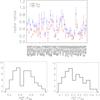 |
Fig. 2 Top: for each cluster in the final sample, we show: the ratio between the upper limit of the radial range investigated in the spatial analysis and our estimate of R200 (blue circles); the ratio between the maximum radial extension of the spectral analysis and R200 (red diamonds). Bottom: distributions of the radial ratios. |
As usual in the X-ray analysis, the estimate of R200 exceeds the radial extension of the spatial and spectral analyses in almost all cases. For the  ratio, we measure a median value (1st, 3rd quartiles) of 0.49 (0.30, 0.59) and a median relative dispersion of 21%, while we obtain 0.29 (0.20, 0.40) and a median relative dispersion of 20% for the
  ratio.
This means that we are not able to sample our objects directly up to R200 in both the surface brightness and temperature profiles, as expected given that both the observational strategy and background characterisation were not optimised to this purpose (see e.g. Ettori & Molendi 2011).
However, R200 is treated as a quantity derived from the best-fit parameters of our procedure for the assumed mass model (R200 = rs × c200) and does not imply a direct extrapolation of the mass profile to recover it.
More interesting is to consider the goodness of the fitting procedure. As we quote in the last column of Table 2, the NFW model provides a reasonable description of the cluster gravitational potential for all our clusters. The probability that a random variable from a χ2 distribution with a given degree of freedom is less or equal to the observed χ2 value is 50% (median of the observed distribution)3. We have only one object with a very low probability (<5%; MACS J2228.5+2037) that suggests an over-estimate of the error bars, and no object with a probability larger than 95%. Nonetheless, deviations are expected in a sample of about 50 clusters and this object has also been considered in the following analysis.
4.2. Comparison with lensing estimates
A useful test for the reliability of our hydrostatic mass estimates is the comparison with results from lensing. The LC2-single catalogue is a collection of 506 galaxy clusters from the literature with mass measurements based on weak lensing (Sereno 2015). Cluster masses in LC2-single are uniformed to our reference cosmology. By cross-matching with the LC2 catalogue4 we find that 32 out of 47 clusters of our sample have weak-lensing reconstructed mass.
 |
Fig. 3 Comparison on the mass estimates within 1 Mpc (left) and R200 (right) for the objects in common between our sample of X-ray measurements and those available in the lensing LC2-single catalogue. |
 |
Fig. 4 Comparison between our constraints from X-ray data and CLASH lensing estimates for the 7 objects in common on the mass concentrations (left) and c − M distribution (right). |
To assess the agreement between the two measurements, we adopt two methods. First, we consider the (natural) logarithm of the mass ratios (Rozo et al. 2014; Sereno & Ettori 2015a). We consider the backwards method masses. This estimator is not affected by the exchange of numerator and denominator. Since quoted errors in compiled catalogs may account for different sources of statistical and systematic uncertainties and published uncertainties are unable to account for the actual variance seen in sample pairs, we conservatively perform an unweighted analysis.
The agreement between mass estimates is good; see Fig. 3. For the masses at R200, we measure a ratio ln(MX/Mlens) = 0.16 ± 0.65, where the first estimate is the median and the second is the dispersion of the distribution of mass ratios. Mass differences are inflated when computed at R200 owing to the different volumes. We then also consider the masses enclosed within a fixed physical radius, 1 Mpc. We find ln(MX/Mlens) = 0.01 ± 0.45.
Seven clusters of our sample are also covered with ground weak-lensing studies by the CLASH programme. Umetsu et al. (2016) perform a joint shear-and-magnification, weak-lensing analysis with additional strong lensing constraints of a subsample of 16 X-ray regular and 4 high-magnification galaxy clusters in the redshift range 0.19 ≲ z ≲ 0.69. For these clusters, we find ln(MX/Mlens) = 0.12 ± 0.58 at R200 and ln(MX/Mlens) = −0.32 ± 0.74 within 1 Mpc, which is consistent with the full lensing sample.
Concentrations are consistent as well; see Fig. 4. For the seven CLASH clusters, we find ln(c200,X/c200,lens) = 0.19 ± 0.53.
As a second method, we estimate the mass bias by regressing the hydrostatic against the lensing masses. We follow the approach detailed in Sereno & Ettori (2015a,b), which accounts for heteroscedastic errors, time dependence, and intrinsic scatter in both the independent and response variable. This accounts for both Mlens and MX being scattered proxy of the true mass. We fit the data with the model MX,200 = α + βMlens,200 + γlog (1 + z). First, we assume that the mass ratio MX,200/Mlens,200 is constant at given redshift (β = 1) and we find α = 0.08 ± 0.15. This bias is consistent with what found with the mass-ratio approach described before. The value γ is consistent with zero, γ = −0.15 ± 0.75, i.e. we cannot detect any redshift dependence in the bias. For the scatters, we find σlog (Mlens,200) = 0.11 ± 0.07 and σlog (MX,200) = 0.04 ± 0.04. Then, we check the above assumption by letting the slope free. We find α = 0.40 ± 0.28, β = 0.74 ± 0.20, γ = −0.32 ± 0.73, σlog (Mlens,200) = 0.08 ± 0.07, and σlog (MX,200) = 0.07 ± 0.05. The slope β is fully consistent with one and the other parameters are in full agreement with the determination assuming β = 1.
We conclude that the X-ray masses are in very good agreement with the lensing masses, MX,200/Mlens,200 ~ 1. Uncertainties are too large to make statements about deviations from equilibrium or non-thermal contributions that can bias the results towards low X-ray masses (Sereno & Ettori 2015a).
5. The concentration-mass relation
 |
Fig. 5 Left: concentration–mass relation obtained for the final cluster sample in the case Δ = 200 (black diamonds). The cluster total masses are obtained following the backwards method described in Ettori et al. (2002). A NFW profile is adopted to describe the gravitational potential. We overplot the c200 − M200 relations predicted by P12 (yellow lines), DM14 (blue lines), and DK15 (red lines). They are calculated for z = 0.4 (dotted lines) and z = 1.2 (dashed lines), which are the lowest and highest redshifts in the sample. Right: the same as the left panel, but here the sample is divided into 7 mass bins. For each bin, error-weighted means for concentration and mass are calculated (black diamonds) and the error bars represent the errors on the weighted means. |
We present our results on the c200 − M200 relation. We stress that our sample, because of the adopted selection criteria (discussed in Sect. 2), is not statistically complete, but represents well the high-mass end of the cluster population even at high redshift (see also discussion in Sect. 6.1).
The concentration-mass relation for the 47 clusters of our sample is shown in Fig. 5. The large error bars are due to the uncertainties in determining the observable surface brightness and spectrum of each cluster, which are consistently propagated up to the concentration and mass derivation.
The right panel of Fig. 5 is obtained by dividing the sample into seven mass bins and estimating, for each bin, the error-weighted mean of the values of the concentration and error on the mean. This operation is made to enhance the observed signal, giving more weight to more precise measurements and to find the mean properties of the sample.
Overall, our data confirm the expected trend of lower concentrations corresponding to higher masses. We investigate the distribution of the concentrations for clusters in two mass ranges below and above the median value of M200 = 1.3 × 10¹⁵M⊙, respectively. The overall distribution is well approximated by a log-normal function with a mean value ⟨ log c200 ⟩ and a scatter σ, ![\begin{eqnarray} \small P(\log c_{200})= \frac{1}{\sigma \sqrt{2\pi}} \exp{\left[-\frac{1}{2}\left(\frac{\log c_{200}-\langle\log c_{200}\rangle}{\sigma}\right)^2\right]}\cdot \end{eqnarray}](/articles/aa/full_html/2016/06/aa27630-15/aa27630-15-eq724.png) (7)We obtain a mean value for the total concentration distribution of ⟨ log c200 ⟩ = 0.60 and a scatter of σ(log c200) = 0.15. By considering the two mass ranges, we find a mean of ⟨ log c200 ⟩ = 0.66 (0.54) and a scatter of 0.14 (0.12) for the low- (high-) mass case. The central peak is shifted towards the low concentrations in the high-mass case, as expected, while we have a slightly larger scatter in the low-mass case. We also investigate the distribution of the concentrations in two redshift ranges, considering the median redshift of the sample, z = 0.6 as threshold. We find a mean of ⟨ log c200 ⟩ = 0.55 (0.66) and a scatter of σ(log c200) = 0.14 (0.13) for the low (high) redshift case, consistent with the above estimates.
(7)We obtain a mean value for the total concentration distribution of ⟨ log c200 ⟩ = 0.60 and a scatter of σ(log c200) = 0.15. By considering the two mass ranges, we find a mean of ⟨ log c200 ⟩ = 0.66 (0.54) and a scatter of 0.14 (0.12) for the low- (high-) mass case. The central peak is shifted towards the low concentrations in the high-mass case, as expected, while we have a slightly larger scatter in the low-mass case. We also investigate the distribution of the concentrations in two redshift ranges, considering the median redshift of the sample, z = 0.6 as threshold. We find a mean of ⟨ log c200 ⟩ = 0.55 (0.66) and a scatter of σ(log c200) = 0.14 (0.13) for the low (high) redshift case, consistent with the above estimates.
In Fig. 5, we also compare our data with three recent results from numerical simulations: Diemer & Kravtsov (2015, hereafter DK15), Dutton & Macciò (2014, hereafter DM14), Prada et al. (2012, hereafter P12). The range of the predicted results is delimited by a dotted line, corresponding to the lowest redshift in the sample (z = 0.4), and a dashed line, corresponding to the highest redshift in the sample (z = 1.2). The comparison with these theoretical works is carried out using the public code Colossus provided by DK155. It is a versatile code that implements a collection of models for the c − M relation, including those of interest here, allowing the choice of a set of cosmological parameters and the conversion among different mass definitions. It turns out to be very useful for our purpose to homogenise the results presented in the original papers to our cosmological model of reference and to masses defined at Δ = 200 with respect to the critical density of the Universe, as in our analysis.
However, it must be noted that we investigate a mass range that might exceed those probed by numerical simulations slightly, in particular, at z ~ 1. In fact, there are no numerical predictions for the behaviour of the c − M relation for masses larger than 1015M⊙ in the range of redshifts considered in our work. We proceed using the numerical predictions as extrapolated from the available datasets6 to compare with our results.
In order to quantify the deviations from numerical predictions, we use the following χ2 estimator: 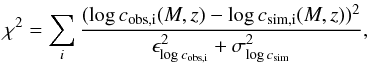 (8)where the sum is carried out over the 47 clusters of our sample; cobs and ϵcobs are the estimates of concentrations and corresponding errors, respectively, listed in Table 2 (we omit the label “200” to simplify the notation); csim are the values derived from the models for fixed mass and redshift; and σlog csim is the intrinsic scatter on the simulated concentrations, assumed to be equal to 0.11 (e.g. DM14). We obtain a χ2 of 272.4, 26.3, and 69.4 when the models by P12, DM14, and DK15, respectively, are considered. A random variable from the χ2 distribution in Eq. (8) with 47 degrees of freedom has a probability of 100, 0.6, and 98 per cent to be lower than the measured values, respectively, indicating a tension with the P12 and DK15 models in the mass (1014 − 4 × 10¹⁵M⊙) and redshift (0.4−1.2) ranges investigated in the present analysis.
It is clear from the right panel of Fig. 5 that our results show the lowest concentrations for the highest masses and are not compatible with an upturn at high masses. This is indeed expected for a sample of relaxed clusters only (see e.g. Ludlow et al. 2012; Correa et al. 2015). The models considered here characterise different halo samples: P12 and DK15 include all the halos, regardless their degree of virialisation, whereas DM14 exclude the unrelaxed halos. Even though the selection is different, we consider objects that show no major mergers and are closer to the selection for relaxed halos applied in numerical simulations. Moreover, the concentrations calculated in P12 are derived from the circular ratio Vmax/V200, rather than from a direct fit to the mass profile and the halos are binned according to their maximum circular velocity, rather than in mass. As pointed out in Meneghetti & Rasia (2013), such methodological differences lead to large discrepancies both in the amplitude and in the shape of the c − M relation, especially on the scales of galaxy clusters, making the comparison with the predictions in P12 not straightforward.
5.1. Evolution with redshift
 |
Fig. 6 Probability distributions of the best-fit parameters of the c − M − z relation Eq. (9) obtained with LIRA, where the covariance between mass and concentration is taken into account. |
With the aim of investigating the dependence of the cluster concentrations on mass and redshift, we consider the three-parameter functional form, c = c0MB(1 + z)C, and we linearly fit our data to the logarithmic form of this function, 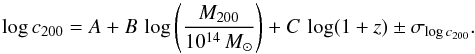 (9)We use the Bayesian linear regression method implemented in the R package LIRA by Sereno (2016). We assume a uniform prior for the intercept A and a Student’s t-prior for both the mass slope B and the slope of the time evolution C. For the intrinsic scatter, we assume that
  follows a gamma distribution. We obtain the following best-fit parameters: A = 1.15 ± 0.29 and B = −0.50 ± 0.20, C = 0.12 ± 0.61 and an intrinsic scatter σlog c200 = 0.06 ± 0.04. This value is lower than the estimates presented in Sect. 5 since here we are correcting for the intrinsic scatter in the hydrostatic masses. The additional correction for this intrinsic scatter of the mass distribution steepens the relation. On the other hand, by taking the covariance between mass and concentration into account, we find a flatter relation, as already pointed out from previous work (e.g. Sereno & Covone 2013).
These values are fully consistent, within the estimated errors, with the IDL routine MLINMIX_ERR by Kelly (2007), which also employs a Bayesian method and with the MPFIT routine in IDL (Williams et al. 2010; Markwardt 2009) that looks for the minimum of the χ2 distribution by taking the errors on both the variables into account. We quote the best-fit values in Table 3. The probability distributions of the best-fit values obtained with LIRA are shown Fig. 6, while the two-dimensional 1-(2-)σ confidence regions are shown in Fig. 7.
Best-fit values of the c − M − z relation.
We measure a normalisation A ≈ 1 and a mass slope B ≈ −0.5 that is lower than the value predicted by numerical simulations (−0.1). By fixing the parameter B to −0.1, we find A = 0.61 ± 0.12, C = 0.38 ± 0.64, and σlog c200 = 0.10 ± 0.02.
 |
Fig. 7 Probability distributions of the best-fit parameters of the c − M − z relation Eq. (9) obtained with LIRA, where the covariance between mass and concentration is taken into account. The thick (thin) lines include the 1-(2-)σ confidence region in two dimensions, here defined as the region within which the value of the probability is larger than exp [ −2.3/2 ] (exp [ −6.17/2 ]) of the maximum. |
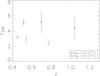 |
Fig. 8 Concentration-redshift relation calculated in two mass ranges: M ≤ 1.33 × 10¹⁵M⊙ (black) and M< 1.33 × 10¹⁵M⊙ (red). For each mass range, the points are the error-weighted means of the concentrations and the error bars are the errors on the means for three redshift bins. The sample is approximately evenly divided in each bin and we show the median redshift for simplicity. |
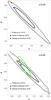 |
Fig. 9 Probability distributions of the A and B parameters of the c − M relation Eq. (9) calculated with LIRA, for the full sample (top) and for the subsample of clusters at z ≥ 0.7 (bottom). The relations are normalised at the median redshift of the sample considered (0.59 and 0.80, respectively). The confidence regions are defined as in Fig. 7. The coloured symbols show the estimates of the parameters from simulations by P12, DM14, and DK15 evaluated at the quoted redshift. The green contour shows the constraints from Sereno & Covone (2013) at 1σ. |
With the Bayesian methods we measure a typical error that is larger by a factor of 2 in normalisation and by a factor of 2.5 in the mass slope with respect to the corresponding values obtained through the covariance matrix of the MPFIT method. All the methods estimate large errors in the redshift dependence and the best-fit values of the redshift slope are consistent with zero (at 1σ level).
The concentration-redshift relation is shown in Fig. 8 for clusters in two mass ranges, considering the median mass 1.33 × 10¹⁵M⊙ as threshold. The sample is divided into three redshift bins for each mass range, which are chosen to have approximately an equal number of clusters in each bin as follows: [0.426−0.583], [0.600−0.734], [0.810−1.235] for the low-mass case, and [0.412−0.494], [0.503−0.591], [0.700−0.888] for the high-mass case. We calculate the error-weighted means of the concentrations and errors on the means for each bin, obtaining 5.06 ± 0.31, 5.18 ± 1.36, 4.39 ± 1.52 for the low-mass case, 3.16 ± 0.27, 2.90 ± 0.42, 2.41 ± 0.37 for the high-mass case. At a fixed mass range, the concentration slightly decreases with redshift, as expected by the fact that the concentration of the cluster is determined by the density of the Universe at the assembly redshift.
Finally, we test the c–M relation in the high redshift regime against the different theoretical models. We use models by P12, DM14, and DK15 to obtain predictions of the measurements of the normalisation and slope of the c − M relation at the median redshift of our sample in the mass range (1014−4 × 10¹⁵M⊙) investigated in the present analysis (we consider 50 log-mass constant points for the fit). As we show in Fig. 9, the predictions from numerical simulations agree well with our constraints, where values from DM14 model are consistent at 1σ level and with larger deviations (but still close to the ~2σ confidence level) associated with the P12 and DK15 expectations.
In particular, once we consider only the 18 clusters of our sample with z ≥ 0.7 and we re-calculate the χ2 estimator in Eq. (8), we obtain 62.3, 6.1, and 17.7 when the models by P12, DM14, and DK15, respectively, are considered. This means that a random variable from the χ2 distribution with 18 degrees of freedom has a probability of 99.9, 0.4, and 52.5 per cent to be lower than the measured values, respectively, indicating that only the P12 model deviates more significantly from our estimates in the (0.7−1.2) redshift range.
6. Sample properties
As discussed in Sect. 2 and 3, a cluster at z> 0.4, and with exposures available in the Chandra archive, is included in our sample if 1) it is observed with sufficient X-ray count statistics to obtain a temperature profile with at least three radial bins; and 2) to a visual inspection of the X-ray maps, it appears to have a regular morphology, so that we can consider it to be close to the hydrostatic equilibrium. Thus, we exclude the objects with a strongly elongated shape or those containing major substructures. Although we do not use any quantitative criterion for this selection, we provide a morphological analysis to present the statistical properties of the sample and to enable comparison with other X-ray samples. We analyse the morphology of each cluster according to the following two indicators: first, the X-ray brightness concentration parameter, cSB, defined as the ratio between the surface brightness, Sb, within a circular aperture of radius 100 kpc and the surface brightness enclosed within a circular aperture of 500 kpc,  (10)and, second, the centroid shift, w, calculated as the standard deviation of the projected separation between the X-ray peak and centroids estimated within circular apertures of increasing radius from 25 kpc to Rap = 500 kpc, with steps of 5%,
 ![\begin{equation} w = \left[ \frac{1}{N-1} \sum_i (\Delta_i - \langle \Delta\rangle)^2 \right]^{1/2} \frac{1}{R_{\rm ap}} , \end{equation}](/articles/aa/full_html/2016/06/aa27630-15/aa27630-15-eq817.png) (11)where Δi is the distance between the X-ray peak and centroid of the ith aperture.
(11)where Δi is the distance between the X-ray peak and centroid of the ith aperture.
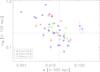 |
Fig. 10 Relation between the X-ray brightness concentration and centroid shift. Dashed lines trace the thresholds indicated by Cassano et al. (2010) to define relaxed and disturbed clusters (see text). Different symbols and colours are used for clusters in different redshift intervals. |
Figure 10 shows that the X-ray concentration is anti-correlated with the centroid shift, qualitatively following the relation found by Cassano et al. (2010). According to their results, clusters with cSB> 0.2 and w< 0.012 are classified as “relaxed” (upper left quadrant in Fig. 10), while those with cSB< 0.2 and w> 0.012, about 1/3 in our sample, are classified as “disturbed” (lower right quadrant). The relative composition of relaxed/disturbed clusters changes with the redshift, as 50% of the clusters observed at z> 0.8 are disturbed.
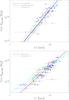 |
Fig. 11 Top panel: relation between the gas mass within R500 and temperature. The black and purple curves show the best-fit relation and its intrinsic scatter obtained for our full and relaxed sample, respectively. The cyan curves represent the relation of Arnaud et al. (2007). Bottom panel: relation between the gas mass within R2500 and temperature. The black curves show the best-fit relation and its intrinsic scatter. The cyan curves represent the relation obtained for the CLASH sample. Coloured symbols as in Fig. 10. |
We characterise the general physical proprieties of the sample by investigating the relation between the mass and temperature of the gas. We consider the error-weighted mean of the temperatures measured in the spectral analysis at radii above 70 kpc. The gas mass is calculated by integrating the gas density profile over a spherical volume of radius R500 evaluated from the mass profile that we constrain as discussed in Sect. 4. We fit the relation  (12)using the Bayesian regression code LIRA of Sereno (2016). We obtain log N = 13.70 ± 0.04 and τ = 1.98 ± 0.18 with an intrinsic scatter σint = 0.134 ± 0.023. Figure 11 shows the Mgas,500 − T relation for the clusters in the sample together with the best-fitting relation, compared to the relation found by Arnaud et al. (2007) for a sample ten morphologically relaxed nearby clusters observed with XMM-Newton in the temperature range 2–9 keV. We find that the two relations are in agreement within the scatter, that in our sample is a factor ~4 higher than that measured for the sample of relaxed local systems in Arnaud et al. (2007). Once we consider only the most “relaxed” systems, that is those identified in the upper left quadrant of Fig. 10, the agreement does not improve. This suggests that more relevant selection biases affect any comparison between our sample and that in Arnaud et al. (2007).
We also compare the same relation with the gas mass estimated within a radius R2500 to the results obtained for the CLASH sample (Postman et al. 2012; Donahue et al. 2014). As shown in Fig. 11, our best-fit relation agrees well with the relation derived for the CLASH clusters with a remarkable agreement on the intrinsic scatter (σint = 0.113 ± 0.008 for our sample, 0.093 ± 0.002 for CLASH).
Overall, we conclude that our sample, spanning a wide range both in redshift (0.41−1.24) and in the dynamical properties as inferred from proxies based on the X-ray morphology, is certainly less homogeneous than the samples of local massive objects. Our sample, however, compares in its physical properties to, for example the CLASH systems, which were only selected to be X-ray morphologically not disturbed and massive (i.e. very X-ray luminous) at intermediate to high redshifts similar to the manner in which we select our targets.
6.1. On the completeness of the sample
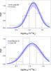 |
Fig. 12 Mass distribution of the selected clusters in two redshift bins. The black histogram bins the observed masses. The blue line is the normal approximation estimated from the regression at the median redshift (see text for details). The shaded blue region encloses the 68.3 per cent probability region around the median relation due to parameter uncertainties. Redshift increases from top to bottom panel. The median and boundaries of the redshift bins are indicated in the legends of the respective panels. |
Some completeness properties of the selected objects can be studied through the analysis of the mass distribution of the clusters in the sample (see Appendix A in Sereno & Ettori 2015b). In so far as the mass distribution is well approximated by a regular and peaked distribution, the completeness of the observed sample can be usually approximated as a complementary error function  (13)where μ is logarithm of the mass. At first order, μχ and σχ can be approximated by the mean and standard deviation of the observed mass distribution.
We perform the analysis of the completeness together with the c − M relation, as LIRA fits the scaling parameters and distribution of the covariate at the same time. The mass distribution for the observed masses is estimated from the regression output, i.e. the function of the true masses, by smoothing the prediction with a Gaussian whose variance is given by the quadratic sum of the intrinsic scatter of the (logarithmic) mass with respect to the true temperature and median observational uncertainty. In Fig. 12, we plot the mass distributions in two redshifts bins and we show that the log-normal distribution provides an acceptable approximation to these mass distributions.
In Fig. 13, we plot the redshift dependence of the selected clusters. The mass completeness limits are fairly constant, differently to survey selected clusters, where the mass limits usually increase with the distance. The selection criteria we imposed on the temperature profile and morphological properties effectively selected the very massive high end of the cluster halo function in the investigated redshift range.
Notwithstanding some heterogeneity in the selection criteria, the sample is well behaved, suggesting that the targeted observations of X-ray clusters cover the very luminous end at each redshift. The effective flux threshold decreases with redshift so that the number of high redshift objects is comparable to the number of intermediate redshift objects.
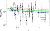 |
Fig. 13 Completeness functions compared to the distribution of the selected clusters in the M200 − z plane (black points). The full lines plot the true value of mass (see text and Appendix A in Sereno & Ettori 2015b for details) below which a given fraction (from top to bottom: 85, 50, and 15 per cent levels, respectively) of the selected sample is contained. The shaded green region encloses the 68.3 per cent confidence region around the 50 per cent level due to uncertainties on the parameters. |
7. Summary and conclusions
We investigate the concentration-mass relation for a sample of 47 galaxy clusters observed with Chandra in the redshift range 0.4 <z< 1.2. We consider the largest sample investigated so far at z> 0.4 and we provide the first constraint on the c(M) relation at z> 0.7 from X-ray data only.
We select archival exposures of targets with no major mergers and with sufficient X-ray signal to allow us to recover the hydrostatic mass properly. Using X-ray morphological estimators, we verify that about 1/3 of the sample is not completely relaxed and that this fraction rises to 0.5 in the objects at z> 0.8.
As consequence of our selection, the sample is not statistically complete and includes targets that were selected differently for their original observations. This implies that some unquantifiable bias could be present and could affect the interpretation of the results. However, we verify that the sample presents a Mgas − T relation that behaves very similarly to the relation estimated locally (see Sect. 6), and that because the selected objects are very luminous in the X-ray band, the selection applied is, in practice, on the total mass and tends to represent the very massive high end of the cluster halo function properly, in particular at high redshift (see Sect. 6.1).
We perform a spatial and a spectral analysis for each cluster, and we extract the radial profiles of the gas temperature and density (obtained from the geometrical deprojection of the surface brightness). We reconstruct the total mass profile by assuming spherical symmetry of the ICM and hydrostatic equilibrium between the ICM and the gravitational potential of the cluster, which is assumed to have a NFW profile described by a scale radius rs and a concentration c. We obtain constraints on (rs,c) by minimising a merit function in which the spectral temperature profile is matched with the temperature predicted from the inversion of the hydrostatic equilibrium equation that depends only on these parameters.
We are able to determine temperature profiles up to a median radius of 0.3 R200 and gas density profiles up to a median radius of 0.5 R200. Beyond these limits, and at R200 in particular, our estimates are the result of an extrapolation. Our hydrostatic mass estimates are in very good agreement with the result from weak-lensing analysis available in literature. In particular, the c − M relation calculated for the clusters shared with the CLASH sample is fully consistent within the errors.
We estimate a total mass M200 in the range (1st and 3rd quartile) 8.1−18.6 × 10¹⁴M⊙ and a concentration c200 between 2.7 and 5. The distribution of concentrations is well approximated by a log-normal function in all the mass and redshift ranges investigated.
Our data confirm the expected trend of lower concentrations for higher mass systems and, at a fixed mass range, lower concentrations for higher redshift systems. The fit to the linear function log c200 = A + B × log M200/ (1014M⊙) + C × log (1 + z) ± σlog c200) gives a normalisation A = 1.15 ± 0.29; a slope B = −0.50 ± 0.20, which is slightly steeper than the value predicted by numerical simulations (B ~ −0.1); a redshift evolution C = 0.12 ± 0.61, which is consistent with zero; and an intrinsic scatter on the concentration σlog c200 = 0.06 ± 0.04.
The predictions from numerical simulations of the estimates of the normalisation A and slope B are in a reasonable agreement with our observational constraints at z> 0.4, once the correlation between them is fully considered (see Fig. 9). Values from Dutton & Macciò (2014) are consistent at the 1σ level. Larger deviations, but still close to the ~2σ level of confidence, are associated with the predictions from Diemer & Kravtsov (2015) and Prada et al. (2012), where the latter is more in tension with our measurements.
In the redshift range 0.8 <z< 1.5, constraints on the c − M relation were also derived in Sereno & Covone (2013) for a heterogeneous sample of 31 massive galaxy clusters with weak- and strong-lensing signals, obtaining similar results to those discussed here with a slope that is slightly steeper than the theoretical expectation.
With this analysis, which represents one of the most precise determinations of the hydrostatic mass concentrations in high-z galaxy clusters, we characterise the high-mass end of the distribution of galaxy clusters even at z ~ 1, which is a regime that is hardly accessible to the present numerical simulations.
A homogeneous sample, and dedicated X-ray follow-up, would improve any statistical evidence presented in our study. In particular, an extension of this analysis to lower redshifts, still using Chandra data consistently, and a careful identification of a subsample of the most relaxed systems would constrain, at higher confidence, any evolution in the concentration-mass relation for clusters of galaxies, also as function of their dynamical state.
We use the LC2-single_v2.0.dat version publicly available at http://pico.bo.astro.it/~sereno/CoMaLit/LC2/
Acknowledgments
We thank Benedikt Diemer and the anonymous referee for helpful comments that improved the presentation of the work. S.E. and M.S. acknowledge the financial contribution from contracts ASI-INAF I/009/10/0 and PRIN-INAF 2012 “A unique dataset to address the most compelling open questions about X-Ray Galaxy Clusters”. M.S. also acknowledges financial contributions from PRIN INAF 2014 “Glittering Kaleidoscopes in the sky: the multifaceted nature and role of galaxy clusters”. This research has made use of the NASA/IPAC Extragalactic Database (NED), which is operated by the Jet Propulsion Laboratory, California Institute of Technology, under contract with the National Aeronautics and Space Administration.
References
- Arnaud, K. A. 1996, Astronomical Data Analysis Software and Systems V, 101, 17 [NASA ADS] [Google Scholar]
- Arnaud, M., Pointecouteau, E., & Pratt, G. W. 2007, A&A, 474, L37 [NASA ADS] [CrossRef] [EDP Sciences] [Google Scholar]
- Bhattacharya, S., Habib, S., Heitmann, K., & Vikhlinin, A. 2013, ApJ, 766, 32 [NASA ADS] [CrossRef] [Google Scholar]
- Binney, J., & Tremaine, S. 1987, Galactic Dynamics (Princeton University Press) [Google Scholar]
- Buote, D. A., Gastaldello, F., Humphrey, P. J., et al. 2007, ApJ, 664, 123 [NASA ADS] [CrossRef] [Google Scholar]
- Cash, W. 1979, ApJ, 228, 939 [NASA ADS] [CrossRef] [Google Scholar]
- Cassano, R., Ettori, S., Giacintucci, S., et al. 2010, ApJ, 721, L82 [NASA ADS] [CrossRef] [Google Scholar]
- Correa, C. A., Wyithe, J. S. B., Schaye, J., & Duffy, A. R. 2015, MNRAS, 452, 1217 [NASA ADS] [CrossRef] [Google Scholar]
- De Boni, C., Ettori, S., Dolag, K., & Moscardini, L. 2013, MNRAS, 428, 2921 [NASA ADS] [CrossRef] [Google Scholar]
- Dickey, J. M., & Lockman, F. J. 1990, ARA&A, 28, 215 [NASA ADS] [CrossRef] [MathSciNet] [Google Scholar]
- Diemer, B., & Kravtsov, A. V. 2015, ApJ, 799, 108 [NASA ADS] [CrossRef] [Google Scholar]
- Dolag, K., Bartelmann, M., Perrotta, F., et al. 2004, A&A, 416, 853 [NASA ADS] [CrossRef] [EDP Sciences] [Google Scholar]
- Donahue, M., Voit, G. M., Mahdavi, A., et al. 2014, ApJ, 794, 136 [NASA ADS] [CrossRef] [Google Scholar]
- Duffy, A. R., Schaye, J., Kay, S. T., & Dal la Vecchia, C. 2008, MNRAS, 390, L64 [NASA ADS] [CrossRef] [Google Scholar]
- Dutton, A. A., & Macciò, A. V. 2014, MNRAS, 441, 3359 [NASA ADS] [CrossRef] [Google Scholar]
- Ettori, S., & Molendi, S. 2011, Mem. Soc. Astron. It. Supp., 17, 47 [Google Scholar]
- Ettori, S., De Grandi, S., & Molendi, S. 2002, A&A, 391, 841 [NASA ADS] [CrossRef] [EDP Sciences] [Google Scholar]
- Ettori, S., Gastaldello, F., Leccardi, A., et al. 2010, A&A, 524, A68 [NASA ADS] [CrossRef] [EDP Sciences] [Google Scholar]
- Ettori, S., Donnarumma, A., Pointecouteau, E., et al. 2013, Space Sci. Rev., 177, 119 [NASA ADS] [CrossRef] [Google Scholar]
- Fruscione, A., McDowell, J. C., Allen, G. E., et al., 2006, Proc. SPIE, 6270, 62701V [CrossRef] [Google Scholar]
- Hennawi, J. F., Gladders, M. D., Oguri, M., et al. 2008, AJ, 135, 664 [NASA ADS] [CrossRef] [Google Scholar]
- Kelly, B. C. 2007, ApJ, 665, 1489 [NASA ADS] [CrossRef] [Google Scholar]
- Klypin, A., Yepes, G., Gottlober, S., Prada, F., & Hess, S., 2014, MNRAS, submitted [arXiv:1411.4001] [Google Scholar]
- Ludlow, A. D., Navarro, J. F., Li, M., et al. 2012, MNRAS, 427, 1322 [NASA ADS] [CrossRef] [Google Scholar]
- Ludlow, A. D., Navarro, J. F., Angulo, R. E., et al. 2014, MNRAS, 441, 378 [NASA ADS] [CrossRef] [Google Scholar]
- Mahdavi, A., Hoekstra, H., Babul, A., et al. 2007, ApJ, 664, 162 [NASA ADS] [CrossRef] [Google Scholar]
- Mahdavi, A., Hoekstra, H., Babul, A., et al. 2013, ApJ, 767, 116 [NASA ADS] [CrossRef] [Google Scholar]
- Mantz, A., & Allen, S. W., 2011, MNRAS, submitted [arXiv:1106.4052] [Google Scholar]
- Markwardt, C. B. 2009, Astronomical Data Analysis Software and Systems XVIII, 411, 251 [NASA ADS] [Google Scholar]
- Mazzotta, P., Rasia, E., Moscardini, L., & Tormen, G. 2004, MNRAS, 354, 10 [NASA ADS] [CrossRef] [Google Scholar]
- Meneghetti, M., & Rasia, E. 2013, MNRAS, submitted [arXiv:1303.6158] [Google Scholar]
- Meneghetti, M., Rasia, E., Vega, J., et al. 2014, ApJ, 797, 34 [NASA ADS] [CrossRef] [Google Scholar]
- Merten, J., Meneghetti, M., Postman, M., et al. 2015, ApJ, 806, 4 [NASA ADS] [CrossRef] [Google Scholar]
- Muñoz-Cuartas, J. C., Macciò, A. V., Gottlober, S., Dutton, A. A., 2011, MNRAS 411, 584 [NASA ADS] [CrossRef] [Google Scholar]
- Navarro, J. F., Frenk, C. S., & White, S. D. M. 1997, ApJ, 490, 493 [NASA ADS] [CrossRef] [Google Scholar]
- Nelson, K., Lau, E. T., Nagai, D., Rudd, D. H., & Yu, L. 2014, ApJ, 782, 107 [NASA ADS] [CrossRef] [Google Scholar]
- Okabe, N., Takada, M., Umetsu, K., Futamase, T., & Smith, G. P. 2010, PASJ, 62, 811 [NASA ADS] [Google Scholar]
- Poole, G. B., Fardal, M. A., Babul, A., et al. 2006, MNRAS, 373, 881 [NASA ADS] [CrossRef] [Google Scholar]
- Postman, M., Coe, D., Benítez, N., et al. 2012, ApJS, 199, 25 [NASA ADS] [CrossRef] [Google Scholar]
- Prada, F., Klypin, A. A., Cuesta, A. J., Betancort-Rijo, J. E., & Primack, J. 2012, MNRAS, 423, 3018 [NASA ADS] [CrossRef] [Google Scholar]
- Rasia, E., Ettori, S., Moscardini, L. et al. 2006, MNRAS, 369, 2013 [NASA ADS] [CrossRef] [Google Scholar]
- Rozo, E., Rykoff, E. S., Bartlett, J. G., & Evrard, A. 2014, MNRAS, 438, 49 [NASA ADS] [CrossRef] [Google Scholar]
- Schmidt, R. W., & Allen, S. W. 2007, MNRAS, 379, 209 [NASA ADS] [CrossRef] [Google Scholar]
- Sereno, M. 2015, MNRAS, 450, 3665 [NASA ADS] [CrossRef] [Google Scholar]
- Sereno, M. 2016, MNRAS, 455, 2149 [NASA ADS] [CrossRef] [Google Scholar]
- Sereno, M., & Covone, G. 2013, MNRAS, 434, 878 [NASA ADS] [CrossRef] [Google Scholar]
- Sereno, M., & Ettori, S. 2015a, MNRAS, 450, 3633 [NASA ADS] [CrossRef] [Google Scholar]
- Sereno, M., & Ettori, S., 2015b, MNRAS, 450, 3675 [NASA ADS] [CrossRef] [Google Scholar]
- Sereno, M., Giocoli, C., Ettori, S., & Moscardini, L. 2015, MNRAS, 449, 2024 [NASA ADS] [CrossRef] [Google Scholar]
- Umetsu, K., Zitrin, A., Gruen, D., et al., 2016, ApJ, 821, 116 [Google Scholar]
- Vikhlinin, A., McNamara, B. R., Forman, W., et al. 1998, ApJ, 502, 558 [NASA ADS] [CrossRef] [Google Scholar]
- Vikhlinin, A., Kravtsov, A., Forman, W., et al. 2006, ApJ, 640, 691 [NASA ADS] [CrossRef] [Google Scholar]
- Williams, M. J., Bureau, M., & Cappellari, M. 2010, MNRAS, 409, 1330 [NASA ADS] [CrossRef] [Google Scholar]
Appendix A: The observed radial profiles of gas density and temperature
We present here the deprojected density and spectral temperature profiles of all of the clusters analysed in this work, as described in Sect. 3.
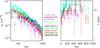 |
Fig. A.1 Deprojected electron density (left) and spectral temperature (right) profiles for clusters in the redshift range 0.405−0.472. |
All Tables
All Figures
|
Fig. 1 Top: comparison between mass estimates obtained following the forwards method (Mfor) and backwards method (Mback) for the 47 clusters of our sample. The lower panel shows the Mfor/Mback ratio of individual clusters against Mback. The dashed line shows the one-to-one relation. The comparison is made at the outermost radius measured in the spectral analysis for each cluster. Middle: distribution of the mass ratios. Bottom: distribution of the relative errors. |
| In the text | |
|
Fig. 2 Top: for each cluster in the final sample, we show: the ratio between the upper limit of the radial range investigated in the spatial analysis and our estimate of R200 (blue circles); the ratio between the maximum radial extension of the spectral analysis and R200 (red diamonds). Bottom: distributions of the radial ratios. |
| In the text | |
|
Fig. 3 Comparison on the mass estimates within 1 Mpc (left) and R200 (right) for the objects in common between our sample of X-ray measurements and those available in the lensing LC2-single catalogue. |
| In the text | |
|
Fig. 4 Comparison between our constraints from X-ray data and CLASH lensing estimates for the 7 objects in common on the mass concentrations (left) and c − M distribution (right). |
| In the text | |
|
Fig. 5 Left: concentration–mass relation obtained for the final cluster sample in the case Δ = 200 (black diamonds). The cluster total masses are obtained following the backwards method described in Ettori et al. (2002). A NFW profile is adopted to describe the gravitational potential. We overplot the c200 − M200 relations predicted by P12 (yellow lines), DM14 (blue lines), and DK15 (red lines). They are calculated for z = 0.4 (dotted lines) and z = 1.2 (dashed lines), which are the lowest and highest redshifts in the sample. Right: the same as the left panel, but here the sample is divided into 7 mass bins. For each bin, error-weighted means for concentration and mass are calculated (black diamonds) and the error bars represent the errors on the weighted means. |
| In the text | |
|
Fig. 6 Probability distributions of the best-fit parameters of the c − M − z relation Eq. (9) obtained with LIRA, where the covariance between mass and concentration is taken into account. |
| In the text | |
|
Fig. 7 Probability distributions of the best-fit parameters of the c − M − z relation Eq. (9) obtained with LIRA, where the covariance between mass and concentration is taken into account. The thick (thin) lines include the 1-(2-)σ confidence region in two dimensions, here defined as the region within which the value of the probability is larger than exp [ −2.3/2 ] (exp [ −6.17/2 ]) of the maximum. |
| In the text | |
|
Fig. 8 Concentration-redshift relation calculated in two mass ranges: M ≤ 1.33 × 10¹⁵M⊙ (black) and M< 1.33 × 10¹⁵M⊙ (red). For each mass range, the points are the error-weighted means of the concentrations and the error bars are the errors on the means for three redshift bins. The sample is approximately evenly divided in each bin and we show the median redshift for simplicity. |
| In the text | |
|
Fig. 9 Probability distributions of the A and B parameters of the c − M relation Eq. (9) calculated with LIRA, for the full sample (top) and for the subsample of clusters at z ≥ 0.7 (bottom). The relations are normalised at the median redshift of the sample considered (0.59 and 0.80, respectively). The confidence regions are defined as in Fig. 7. The coloured symbols show the estimates of the parameters from simulations by P12, DM14, and DK15 evaluated at the quoted redshift. The green contour shows the constraints from Sereno & Covone (2013) at 1σ. |
| In the text | |
|
Fig. 10 Relation between the X-ray brightness concentration and centroid shift. Dashed lines trace the thresholds indicated by Cassano et al. (2010) to define relaxed and disturbed clusters (see text). Different symbols and colours are used for clusters in different redshift intervals. |
| In the text | |
|
Fig. 11 Top panel: relation between the gas mass within R500 and temperature. The black and purple curves show the best-fit relation and its intrinsic scatter obtained for our full and relaxed sample, respectively. The cyan curves represent the relation of Arnaud et al. (2007). Bottom panel: relation between the gas mass within R2500 and temperature. The black curves show the best-fit relation and its intrinsic scatter. The cyan curves represent the relation obtained for the CLASH sample. Coloured symbols as in Fig. 10. |
| In the text | |
|
Fig. 12 Mass distribution of the selected clusters in two redshift bins. The black histogram bins the observed masses. The blue line is the normal approximation estimated from the regression at the median redshift (see text for details). The shaded blue region encloses the 68.3 per cent probability region around the median relation due to parameter uncertainties. Redshift increases from top to bottom panel. The median and boundaries of the redshift bins are indicated in the legends of the respective panels. |
| In the text | |
|
Fig. 13 Completeness functions compared to the distribution of the selected clusters in the M200 − z plane (black points). The full lines plot the true value of mass (see text and Appendix A in Sereno & Ettori 2015b for details) below which a given fraction (from top to bottom: 85, 50, and 15 per cent levels, respectively) of the selected sample is contained. The shaded green region encloses the 68.3 per cent confidence region around the 50 per cent level due to uncertainties on the parameters. |
| In the text | |
|
Fig. A.1 Deprojected electron density (left) and spectral temperature (right) profiles for clusters in the redshift range 0.405−0.472. |
| In the text | |
 |
Fig. A.2 Same as in Fig. A.1 for clusters in the redshift range 0.494−0.546. |
| In the text | |
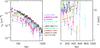 |
Fig. A.3 Same as in Fig. A.1 for clusters in the redshift range 0.548−0.7. |
| In the text | |
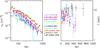 |
Fig. A.4 Same as in Fig. A.1 for clusters in the redshift range 0.7−0.813. |
| In the text | |
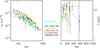 |
Fig. A.5 Same as in Fig. A.1 for clusters in the redshift range 0.831−1.235. |
| In the text | |
Current usage metrics show cumulative count of Article Views (full-text article views including HTML views, PDF and ePub downloads, according to the available data) and Abstracts Views on Vision4Press platform.
Data correspond to usage on the plateform after 2015. The current usage metrics is available 48-96 hours after online publication and is updated daily on week days.
Initial download of the metrics may take a while.