| Issue |
A&A
Volume 587, March 2016
|
|
|---|---|---|
| Article Number | A43 | |
| Number of page(s) | 16 | |
| Section | Extragalactic astronomy | |
| DOI | https://doi.org/10.1051/0004-6361/201527152 | |
| Published online | 15 February 2016 | |
A multi-epoch spectroscopic study of the BAL quasar APM 08279+5255
II. Emission- and absorption-line variability time lags
1
Università degli Studi di Roma “La Sapienza”,
p.le A. Moro 5,
00185
Rome,
Italy
e-mail:
saturnfg@roma1.infn.it
2
Università degli Studi “Roma Tre”, via della Vasca Navale 84, 00146
Rome,
Italy
3
Università di Roma “Tor Vergata”, via della Ricerca Scientifica 1, 00133
Rome,
Italy
4
Università di Bologna, via Zamboni 33, 40126
Bologna,
Italy
5
INAF–IASF Bologna, via Gobetti 101, 40129
Bologna,
Italy
Received: 10 August 2015
Accepted: 4 December 2015
Context. The study of high-redshift bright quasars is crucial to gather information about the history of galaxy assembly and evolution. Variability analyses can provide useful data on the physics of quasar processes and their relation with the host galaxy.
Aims. In this study, we aim to measure the black hole mass of the bright lensed BAL QSO APM 08279+5255 at z = 3.911 through reverberation mapping, and to update and extend the monitoring of its C IV absorption line variability.
Methods. We perform the first reverberation mapping of the Si IV and C IV emission lines for a high-luminosity quasar at high redshift with the use of 138 R-band photometric data and 30 spectra available over 16 years of observations. We also cross-correlate the C IV absorption equivalent width variations with the continuum light curve to estimate the recombination time lags of the various absorbers and infer the physical conditions of the ionised gas.
Results. We find a reverberation-mapping time lag of ~900 rest-frame days for both Si IV and C IV emission lines. This is consistent with an extension of the BLR size-to-luminosity relation for active galactic nuclei up to a luminosity of ~1048 erg s-1, and implies a black hole mass of 1010 M⊙. Additionally, we measure a recombination time lag of ~160 days in the rest frame for the C IV narrow absorption system, which implies an electron density of the absorbing gas of ~2.5 × 104 cm-3.
Conclusions. The measured black hole mass of APM 08279+5255 indicates that the quasar resides in an under-massive host-galaxy bulge with Mbulge ~ 7.5MBH, and that the lens magnification is lower than ~8. Finally, the inferred electron density of the narrow-line absorber implies a distance of the order of 10 kpc of the absorbing gas from the quasar, placing it within the host galaxy.
Key words: galaxies: active / quasars: absorption lines / quasars: emission lines / quasars: supermassive black holes / quasars: individual: APM 08279+5255 / quasars: general
© ESO, 2016
1. Introduction
Quasars are broad-line, high-luminosity active galactic nuclei (AGNs) with spectral features surprisingly similar to those of the Seyfert galaxies despite a difference in luminosity of several orders of magnitude. This implies a common process at the base of their existence. Moreover, quasars distinguish themselves for emitting at all wavelengths from radio to gamma rays with a total energy emission comparable to that of a bright galaxy. The commonly accepted model able to match the observations is the accretion of gas around a supermassive black hole (SMBH; Salpeter 1964; Zel’dovich & Novikov 1965).
The similarity of quasar spectra naturally leads to a unified scenario for the structure of quasars (see e.g. Urry & Padovani 1995 for a review). In the simplest scenario, ionised gas clouds orbit around the black hole at radii larger than the accretion disk responsible for the continuum emission, producing the broad (from a broad line region, BLR, still relatively close to the central black hole) and narrow (from a farther narrow line region, NLR) emission lines. At intermediate orientations between the accretion disk plane and its axis, high-velocity winds can be launched under the action of the radiation pressure, thus originating the broad absorption line (BAL) phenomenon when the quasar is viewed along the wind (Weymann & Foltz 1983; Turnshek 1988; Elvis 2000).
Assuming that such features are common to all quasars, the only two parameters that the quasar structure depends on are the SMBH mass and the quasar inclination angle with respect to the line of sight. The first quantity has great relevance in cosmological studies: in fact, SMBHs trace large-scale structures and co-evolve with their host galaxies (see e.g. Cattaneo et al. 2009, and refs. therein), thus supplying information about the quantity of matter in the Universe and the history of galaxy assembly.
Currently, the only direct way to estimate the SMBH mass beyond the local Universe is through reverberation mapping (RM; Gaskell & Peterson 1987; Edelson & Krolik 1988; White & Peterson 1994; Peterson 1997) by which the time lag tlag between the quasar broad emission line and continuum variability, hence the size of the BLR RBLR = ctlag, can be measured. Under the hypothesis of virialised orbits in the BLR, the black hole mass MBH is given by  (1)Here, the form factor f summarises all the ignorance about the shape and inclination with respect to the line of sight of the BLR, which can significantly alter the final value of MBH, while Δv is the full width at half maximum (FWHM) of the considered emission line. Under reasonable assumptions about the distribution of gas clouds in the BLR (i.e. assuming some physical value for f), this formula gives a measurement of MBH in principle for all classes of AGNs with broad emission lines. In this way, relations between mass, line width, and quasar luminosity (e.g. McLure & Dunlop 2004; Vestergaard & Peterson 2006; Shen et al. 2011) can be computed, and the SMBH mass can be estimated from single-epoch quasar spectra. This avoids the necessity of a RM for each object, allowing us to obtain mass estimates for a large number of sources.
The application of the RM method was initially limited to low-luminosity, local AGNs such as the Seyfert galaxies, which have variability timescales from days to weeks at most (Wandel et al. 1999; Peterson et al. 2004). Subsequently, this method was applied to low-redshift quasars (z< 0.4; Kaspi et al. 2000). For higher luminosity, higher redshift quasars, the increase of the BLR size with luminosity and the cosmological time dilation increase the variability timescales to years, thus making campaigns for quasar RM observationally expensive. Until now, only three luminous, high-redshift quasars have RM mass measurements (Kaspi et al. 2007; Chelouche et al. 2012; Trevese et al. 2014); this lack of information at high masses and luminosities means that the application of single-epoch mass-luminosity relations to quasars is actually an extrapolation only based on data from AGNs of moderate redshift, making the current black hole mass estimates of quasars in cosmological surveys subject to possible biases (e.g. Shen et al. 2011).
Broad absorption line quasars (BAL QSOs; Lynds 1967; Weymann & Foltz 1983; Turnshek 1988; Elvis 2000) are a very important test for unified scenarios, since the mechanisms to launch a highly ionised, high-velocity (up to ~0.2c) absorbing outflow are still poorly known. The exact location, structure, and physical properties of BAL outflows are difficult to introduce in unification schemes for quasars.
The variability of BALs (e.g. Barlow et al. 1992; Gibson et al. 2008; Capellupo et al. 2011; Trevese et al. 2013) is one of the main ways to gather information about gas producing broad absorption features, such as physical (density, temperature, ionisation) and geometrical (location, opening angle, bending) properties of the outflow. Several programmes to study BAL variability are underway, based either on single objects with multi-year observations (Barlow et al. 1992; Krongold et al. 2010; Hall et al. 2011; Trevese et al. 2013; Grier et al. 2015) or on ensemble analyses of quasar samples with a few (up to 10) observations per object (Barlow 1993; Lundgren et al. 2007; Gibson et al. 2008; Capellupo et al. 2011, 2012, 2013; Filiz Ak et al. 2013). Currently, the possible explanation of the BAL variability over multi-year timescales consider changes either in the gas ionisation level or in the covering factor, although the second possibility is favoured since: (i) the variations tend to occur in narrow portions of BAL troughs (e.g. Filiz Ak et al. 2013); and (ii) they generally do not correlate with changes in the observed continuum (Gibson et al. 2008; Capellupo et al. 2011; but see Trevese et al. 2013).
In this study, we take advantage of our long-term monitoring programme of high-luminosity quasars (Trevese et al. 2007) to improve the statistical database for the bright BAL QSO APM 08279+5255 to update our study on its C IV absorption variability (Trevese et al. 2013; Paper I henceforth; Saturni et al. 2014) and to obtain estimates of its black hole mass through RM of Si IV and C IV emission lines. APM 08279+5255 is one of the most luminous quasars, discovered in 1998 by Irwin et al. (1998). This quasar is well known for its gravitational lensing, and is the first confirmed case of a lens with odd number of image components (Lewis et al. 2002). Additionally, its redshift inferred from the high-ionisation emission lines (N V, Si IV, C IV and C III]) is z = 3.87 (Irwin et al. 1998), which corresponds to an outflow velocity of ~2500 km s-1 with respect to the systemic redshift z = 3.911 derived from the CO emission lines (Downes et al. 1999).
The paper is organised as follows: in Sect. 2, we briefly present the target of the observations and describe the adopted observational strategy and data reduction; in Sect. 3, we present the line-to-continuum RM time lags; in Sect. 4, we update the absorption variability study of APM 08279+5255 with new data; finally, in Sect. 5 we discuss APM 08279+5255 black hole mass estimates and absorption variability, summarising all the findings in Sect. 6. Throughout this paper, we adopt a concordance cosmology with H0 = 70 km s-1 Mpc-1, ΩM = 0.3 and ΩΛ = 0.7.
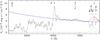 |
Fig. 1 Dereddened spectrum of APM 08279+5255 taken at MJD = 52 695 at the 1.82 m Copernico telescope (Asiago, Italy). Superimposed on the spectrum (black solid line), a power-law continuum (blue dot-dashed line), a Gaussian fit of the C IV emission line (green dashed line), and the combination of these two components into a single pseudo-continuum (red solid line) are shown. The dotted line indicates the flux zero level. The major absorption features are denoted with the identifiers used in the text (see Sect. 4) and ticks. The positions of the Lyman limit at λ912 Å in the rest frame and the major emission lines are also indicated. |
2. Observations and data reduction
2.1. The reverberation mapping campaign
Our RM campaign of luminous quasars started in 2003 at the Asiago Observatory, Italy (Trevese et al. 2007). Motivated by the work of Netzer (2003) concerning the possible biases introduced in galaxy mass estimates by an overestimation of their black hole mass MBH, the goal was to measure MBH of some intrinsically bright objects to extend the BLR size-luminosity relationships for AGNs (Peterson et al. 2005; Kaspi et al. 2007) to luminosities greater than ~1046 erg s-1. Both R-band photometric data and spectra have been obtained with the Asiago Faint Object Spectrograph and Camera (AFOSC) at the 1.82 m Copernico telescope (Asiago, Italy). Since December 2012, the campaign is underway at the 1.52 m Cassini telescope (Loiano, Italy) with the Bologna Faint Object Spectrograph and Camera (BFOSC).
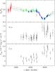 |
Fig. 2 Upper panel: R-band continuum light curve of APM 08279+5255. The Lewis et al. (1999) photometric campaign (red triangles), the Asiago and Loiano (Trevese et al. 2007, 2013, 2014) RM campaign (green dots), and the rescaled V-band Catalina photometry (blue crosses) are all included. Superimposed on the data, the best-fit DRW variability model computed by JAVELIN (Zu et al. 2011) is shown (black solid line) delimited by its error boundaries at 68% probability (black dashed lines). Middle panel: Si IV light curve. Lower panel: C IV light curve. |
The procedure of observation and data reduction is explained in detail in previous papers (Trevese et al. 2007, 2013, 2014). Here we simply recall that the instrument was set in to simultaneously observe the quasar and a star S of comparable magnitude (R = 14.66; Röser et al. 2010), located at α 08 31 22.3 δ +52 44 58.6 (J2000), which has been adopted as a calibration reference for both photometry and spectra. The quasar and the star are observed in the same slit. A wide slit of 8” (on AFOSC) or 12” (on BFOSC) was adopted to avoid light losses due to small misalignments or differential refraction, which would produce artificial variability. With this approach, we obtain differential magnitudes ΔR between the quasar and reference star from the photometry, and spectral ratios Q/S between the uncalibrated quasar (Q) and stellar (S) spectra. These spectral ratios are then multiplied to a spectrum of S taken at MJD = 55 894.5 and calibrated through standard IRAF techniques; assuming that the reference star is non-variable, this provides a flux calibration preserving the quasar variability. An example of these spectra is shown in Fig. 1. In total, we have collected 25 R-band photometric data points and 30 spectra until March 2015, part of which has been already analysed in previous papers focussed on the C IV absorption variability (Paper I; Saturni et al. 2014).
The RM technique requires us to construct a quasar continuum light curve (LC) and an emission-line LC for each line considered. Therefore, we have converted our magnitude differences ΔR between quasar and reference star to flux ratios FQ/FS; since we compute an emission-line contribution to the total R-band flux of only ~11%, we assume that our photometry is tracing the quasar UV rest-frame continuum variability well, and adopt it as the reference to construct APM 08279+5255 continuum LC. We have then computed the quasar continuum flux from our series of spectra in a rest-frame spectral interval of 100 Å around λ = 1350 Å. The LC obtained with this approach only differs from the R-band photometry by a scale factor; this, assumed constant for all spectra, has been computed over a time interval in which the quasar flux level remains approximately constant and has been verified to provide a good match to the R-band photometry in the presence of flux variations as well. Therefore, we have scaled the spectral continuum LC to the photometric data by this factor and have added it to the full data set of the continuum LC. This improves our statistics to 55 points tracing the continuum variations of APM 08279+5255. In Table A.1, we report our spectro-photometric data together with the data collected from the literature described in the next subsection.
2.2. Data from the literature
As in Paper I, we have added the photometric data of Lewis et al. (1999) to our data set, after re-scaling their measurements from their reference star S1, which is always fortuitously included in our field of view, to our reference star S. This provides us with additional 23 photometric points. One last data set of 59 V-band points, scaled to our R-band photometry in the same way as our spectral continuum fluxes, came from the Catalina Sky Survey (Drake et al. 2009). Thus, we end up with a total of 138 continuum data points for APM 08279+5255 along with 30 spectra, which constitutes the largest data set collected for a quasar at such high redshift so far. Table A.1 summarises our observations and the literature data: we provide the observation date MJD −50 000 in Col. 1, the telescope in Col. 2, the observation type (spectroscopic or photometric) in Col. 3, the continuum flux ratios FQ/FS referred to the R-band fluxes (as explained in the previous subsection) in Col. 4, the Si IV and C IV emission-line fluxes in Cols. 5 and 6, respectively (see Sect. 3).
We also take advantage of the existence of five more spectra of APM 08279+5255 available in the literature (Irwin et al. 1998; Ellison et al. 1999; Hines et al. 1999; Lewis et al. 2002; Saturni et al., in prep.), introducing these spectra into our monitoring as well. Unfortunately, because of the lack of a uniform flux calibration, these spectra cannot be used in our RM, and hence are added to the current data set only for the purposes of updating the C IV absorption variability study presented in Paper I and Saturni et al. (2014), which only requires fluxes normalised to the local continuum. We only used the HST/STIS spectrum from Lewis et al. (2002) in the RM for the sole purpose of determining the C IV emission-line width to be used in the RM measurement of APM 08279+5255 SMBH mass. This is motivated by the fact that this spectrum is taken outside the atmosphere, thus avoiding the telluric absorption by the Fraunhofer A band on the residual C IV emission-line wing.
3. Reverberation mapping of the Si IV and C IV emission lines
We are now able to perform the RM of APM 08279+5255 owing to our long-time monitoring. This is carried out by cross-correlating the variability of the R-band flux tracing the continuum with the Si IV and C IV emission-line fluxes to find the most probable lag between continuum and line variations. The LCs to be used in this process, shown in Fig. 2, are constructed as follows.
-
APM 08279+5255 spectrum is reddened by a foreground absorber at z ~ 1 (likely the as yet invisible lensing galaxy; Ellison et al. 2004), with a V-band reddening parameter AV ~ 0.5 mag (Petitjean et al. 2000). We deredden our series of spectra with an extinction law for Small Magellanic Cloud-type dust (Pei 1992) produced at z = 1.062 (Ellison et al. 2004) to obtain a better power-law fit to the continuum. This function is fixed at all epochs, hence, it does not introduce any noise in the variability.
-
For all the spectra, we evaluate the Si IV flux by subtracting a power-law continuum computed at each epoch over two wavelength intervals, λλ6620−6680 and λλ7000−7100 in the observer frame, adjacent to that emission line and free of other emission or absorption features. The Si IV flux is then defined as the integral of the line flux in the interval λλ6680−7000.
-
Finally, we apply the same fitting procedure described in Paper I and Saturni et al. (2014) to the C IV emission line, assumed Gaussian, and compute its line flux as the integral of the resulting fitting function at each epoch. In this procedure, only the line amplitude is allowed to vary, whereas the peak position is fixed to the C IV λ1549 at z = 3.87, and the Gaussian width is fixed to the value σg = 3200 km s-1 obtained through a fit performed onto the HST/STIS high-resolution spectrum (Lewis et al. 2002), which is free of the O2 telluric absorption on the C IV red wing.
We report all the emission-line fluxes in the fifth and sixth columns of Table A.1 together with their 1σ errors.
In order to determine the emission-line time lag, we recall that the usual method consists in evaluating the peak or centroid of the line-to-continuum cross-correlation function (CCF). This can be constructed either by computing a discrete correlation function (DCF; Edelson & Krolik 1988) or via an interpolation of the LCs (ICCF; Gaskell & Peterson 1987; White & Peterson 1994). However, CCFs only provide consistent results for well-sampled LCs, and instead present technical problems in the case of poor sampling (Peterson 1993; Welsh 1999). In particular, the DCF sensitivity to real correlation decreases. An estimate of the confidence interval on the measured time lag can be obtained through the DCF z-transformation method (ZDCF) by Alexander (1997, 2013); however, this requires us to eliminate from each DCF bin all points corresponding to pairs of epochs with measured data in common. Thus, this is hardly applicable in our case, where the sampling is particularly poor.
We therefore evaluate the RM time lags of SI IV and C IV with the JAVELIN code1, based on its previous version SPEAR (Stochastic Process Estimation for AGN Reverberation) by Zu et al. (2011). With respect to traditional CCFs, the advantage of this method, whose statistical bases date back to Press et al. (1992), Rybicki & Press (1992) with a first application in Rybicki & Kleyna (1994), is that it makes use of an interpolation algorithm in which the entire data set contributes to each interpolated point under the assumption that the emission-line LCs Fl(t) are a scaled, smoothed, and delayed version of the continuum LC Fc(t). The quasar continuum LC is then modelled with a damped random walk (DRW) process described by a damping timescale τd and an rms variability amplitude σ (Kelly et al. 2009; Kozłowski et al. 2010; MacLeod et al. 2010; Zu et al. 2013). This is realised through the application of statistical weights that are determined from the auto-correlation functions of the data.
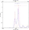 |
Fig. 3 Posterior distributions of the Si IV (blue solid histogram) and C IV (red dashed histogram) RM time lags computed with JAVELIN. The time-lag mean values (blue point and red square) for each distribution are shown together with their corresponding confidence intervals at 68% (colour and line-type codes as per the histograms) and at 95% probability (dotted error bars). |
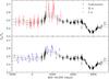 |
Fig. 4 APM 08279+5255 light curve composed with the continuum (black dots) and emission-line fluxes, which are scaled in intensity and shifted in time of their JAVELIN lags of 837 and 901 rest-frame days, respectively, to mimic the original continuum light curve that is reverberated by the quasar BLR. Upper panel: continuum and Si IV (red triangles). Lower panel: continuum and C IV (blue crosses). In both panels, a DRW continuum, fitted by JAVELIN to the data with the damping timescale τd blocked to that of the continuum fit, is shown superimposed to the light curve (solid line) along with its 1σ error band (dashed lines). |
The emission-line LC is obtained from the continuum LC through the convolution with a transfer function Ψ(t)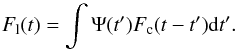 (2)In this analysis, we adopt for Ψ(t) the simple analytic top-hat form as done by Zu et al. (2011), of width Δ and area A, i.e.
 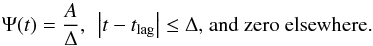 (3)This choice is based on the fact that the resulting emission-line lag tlag does not depend strongly on the specific form of Ψ(t) (Rybicki & Kleyna 1994). A maximum-likelihood code provides the five best-fit parameters (τd, σ, tlag, A and Δ) for the DRW model that describes the continuum LC and the top-hat transfer function. Finally, confidence limits on the fit parameters are obtained through Monte-Carlo Markov chain (MCMC) iterations. With respect to traditional CCFs, the model-dependent nature of JAVELIN has the advantage of producing smaller lag uncertainties (Zu et al. 2011).
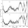 |
Fig. 5 Upper panel: ICCF (solid line) with its 1σ error (grey area) and ZDCF (black points) for the continuum and the Si IV emission line. Lower panel: same as in the upper panel, but for the continuum and the C IV emission line. The ZDCF is computed over 15 uncorrelated points per bin, and finds a simultaneous peak for the two emission features at |

In order to verify that the result of JAVELIN does not depend on the assumed model, we compute the classical ICCF and DCF via its z-transformation (ZDCF) for each pair of lines and continuum LCs, and evaluate the corresponding RM time lags with their uncertainties. Although in our case the CCFs have low statistical significance, they are completely model independent.
The uncertainty on the ICCF lag is estimated by applying the “flux randomisation and random sample selection” method (FR/RSS) by Peterson et al. (1998). This method allows us to compute the statistical distribution of the line-to-continuum time lags by iterating the ICCF procedure over undersampled continuum and emission-line LCs, altering the remaining data by adding a random noise with a Gaussian distribution whose standard deviation is the 1σ error on each measured point. In order to compute the ZDCF time lag and the uncertainty on the peak position, we use the routines made available online by T. Alexander2.
In Sects. 3.1 and 3.2, we respectively report the RM time lags found with the analysis carried out by JAVELIN and those found through the CCFs for comparison.
3.1. Reverberation mapping with JAVELIN
As a first step, we apply the JAVELIN method to study the correlation of the individual Si IV and C IV lines with the continuum. As a result of our unprecedented long-time monitoring, we are able to probe time lags in the observer frame up to ~6000 days, corresponding to ~1200 rest-frame days at z = 3.911. The analysis with JAVELIN gives  days in the observer frame and
  days, thus suggesting that the BLR emitting the Si IV and C IV lines are both located at the same distance from the quasar central engine (~850 light days for APM 08279+5255).
The RM time lags can be also estimated by fitting the LCs of multiple emission lines together with JAVELIN. This is particularly useful when the LC sampling is sparse, since if all emission lines follow the same variability model as the continuum, the available information to fit the variability increases. Therefore, we perform this analysis with the full data set of 138 continuum points and 30 points for each emission line, for a total of Ntot = 198 light-curve points to fit the eight parameters (continuum damping timescale and variability amplitude, two top-hat lags, two smoothing widths, and two scale factors) of the DRW plus top-hat transfer function model of quasar line-to-continuum variability.
The joint fit with JAVELIN gives  days in the observer frame and
  days, respectively. In Fig. 3, we show the posterior distribution of a JAVELIN MCMC run with 1.6 × 10⁵ iterations for these time lags. Also, in Fig. 4 we show the emission-line LCs of Si IV and C IV scaled to the R-band continuum, and shifted back in time of the relevant RM lags. At a first glance, the emission-line LCs are both consistent with the interpolated decrease in the continuum flux after the rise around MJD ~ 51 500 observed by Lewis et al. (1999).
Some caution must be adopted in interpreting the result, since the lag associated with the cross-correlation peak corresponds to a maximum of the emission-line LCs falling in a gap of the continuum LC (see Fig. 4). This is however made possible by the assumption of the method, which uses the information of the emission-line LCs to interpolate the continuum. In the continuum LC gap between 51 500 and 52 500 days, JAVELIN is therefore using the local maximum of the emission-line LCs at MJD ~ 56 000. Such an interpolation is the probable cause of the extension at large time lags of the emission-line lag posterior distribution and, consequently, of the asymmetric errors at 95% probability in the lag estimate (see Fig. 3); nevertheless, the result is plausible. With this measurement, APM 08279+5255 becomes the most distant object, and one of the intrinsically most luminous for which RM time lags are available.
3.2. Reverberation mapping with the CCFs
For comparison with the time lags found by JAVELIN, we also present a CCF analysis of APM 08279+5255 line and continuum LCs. The results are shown in Fig. 5; a peak in the ZDCF appears at  days in the observer frame, which is simultaneous for the Si IV and C IV. However, this peak is located in the last significant ZDCF bin, i.e. a bin containing at least the minimal number of points required to compute a statistically significant ZDCF value. The ZDCF point at a longer lag is already not significant. Coupled with the large bin width of the ZDCF peak, this prevents to compute the 68% probability confidence interval on the peak position over more than one ZDCF bin.
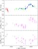 |
Fig. 6 Upper panel: updated time series of APM 08279+5255 R-band differential magnitude with 1σ errors, adding all the photometric data available in literature (same colour code than in the upper panel of Fig. 2). Middle panel: BAL EWs computed for all the existing APM 08279+5255 spectra with 1σ errors. Lower panel: NAL EWs computed for all the existing APM 08279+5255 spectra with 1σ errors. In both middle and lower panels, Irwin et al. (1998; red triangle), Ellison et al. (1999; green cross), Hines et al. (1999; blue circle), Lewis et al. (2002; cyan square) and Saturni et al. (2015; yellow star) spectra are all included along with the Asiago and Loiano spectra (magenta dots). |
We evaluate tlag from the ICCF estimating the lag uncertainty with the FR/RSS method. We obtain  days in the observer frame and
  days. We also quantify the significance of the CCF peaks by performing a Student’s t-test (Bevington 1969; see also Shen et al. 2015), which allows us to evaluate the integral probability of the null hypothesis P( >r,N) for a correlation coefficient r computed over N pairs of data points. We compute this probability for both the ICCFs and ZDCFs: for the ICCFs, we obtain P( >r,N) = 0.03 for the Si IV (r = 0.60, N = 12) and 0.05 for the C IV (r = 0.55, N = 12), respectively; for the ZDCFs, the test gives P( >r,N) = 0.04 for the Si IV (r = 0.53, N = 15) and 0.29 for the C IV (r = 0.21, N = 15). As expected, the CCFs do not provide a statistically significant result; however, the peaks are all located close to the same position obtained with JAVELIN, indicating that the previously found lags are not an artifact of the adopted model.
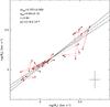 |
Fig. 7 EWs of the two C IV BAL troughs of APM 08279+5255, plotted one versus the other (black points). The red arrows connect consecutive epochs of EW pairs. The two correlation fits of BAL1 versus BAL2 and vice versa are shown (solid lines) along with the corresponding bisector fit ( dot-dashed line). Slope mbis and intercept qbis of such fit, correlation coefficient r, and corresponding null-hypothesis probability p( >r) are reported. The cross in the lower right corner represents the mean error on the data set in each direction. |
4. Update of the C IV absorption variability
The variability of APM 08279+5255 C IV absorption features was presented in Paper I and Saturni et al. (2014). In the present paper, we take advantage of the new observations from the Loiano observatory and the photometric data set from the Catalina Sky Survey to extend the absorption variability monitoring in time, and partially fill the gaps in our time series. The data reduction is identical to that performed in Paper I. Fig. 6 shows the update of the C IV absorption equivalent width (EW) variability of APM 08279+5255 up to MJD = 57 093.
In Paper I, we identified four absorption systems in the C IV region of APM 08279+5255, thanks to the availability of high-resolution spectra. We therefore distinguish two BAL components (labelled BAL1 and BAL2 in Fig. 1) separated by a NAL system (“blue NAL” in Fig. 1) described in Srianand & Petitjean (2000). Another NAL system (“red NAL” in Fig. 1) is located redwards the C IV emission (Srianand & Petitjean 2000; Ellison et al. 2004). With respect to the previous variability analysis, the “blue NAL” has not been included in this update because of the uncertainty in determining the residual contamination of its EW after the subtraction of the two BAL components. We describe the behaviour of the BAL troughs and the “red” NAL in the following subsections.
4.1. The BAL variability
As described in Paper I and Saturni et al. (2014), we considered the sum of the two C IV BAL components as a single absorption feature for the purpose of the EW variability analysis. We adopted this solution since the EWs of such components, computed separately by modelling the BAL profile at low resolution with two Gaussian absorptions, are highly correlated in their variations over the whole monitoring time (see e.g. Fig. 5 in Paper I). We show in Fig. 7 that this correlation is maintained (r = 0.90,p( >r) = 9.0 × 10⁻⁸) to verify that the new data do not change this result. This result is confirmed by computing the discrete cross-correlation function of the two BAL EWs according to the ZDCF algorithm introduced in Sect. 3, which peaks at  days in the observer frame (
 rest-frame days), which is consistent with no lag between the two components.
This simultaneous variability of different BAL troughs associated with different transitions (Brandt et al. 2014) or the same transition (Grier et al. 2015) is observed in some other BAL QSOs, indicating that common physics is driving the BAL variations. We quantify the comparison between BAL1 and BAL2 variability by performing a bisector fit (Akritas & Bershady 1996) of the relation between the logarithmic BAL EWs log W1 and log W2, obtaining  (4)With respect to the simple correlation analyses among R-band magnitudes, BAL and NAL EWs presented in Paper I, we add cross-correlation analyses. To accomplish this, we only apply the ICCF and ZDCF methods since the reverberation model on which JAVELIN is based cannot be directly applied to absorption variability.
We present the results in the left panel of Fig. 8. As expected from a visual inspection of Fig. 6, the correlation peak appears at zero lag ( days in the observer frame with a significance over 3σ level: N = 15, r = 0.94 and P( >r,N) = 2 × 10⁻⁷), since the absorbing gas lies along the line of sight and there is no light-travel lag between the continuum and absorption (Barlow et al. 1992; Barlow 1993). Nonetheless, a physical lag as a result of recombination timescale could be present, but is short for high electron densities.
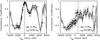 |
Fig. 8 Left panel: cross-correlation function of the R-band magnitudes with the total C IV BAL EW tracing the continuum. Right panel: cross-correlation function of the R-band magnitudes with the total C IV “red” NAL EW. In both panels, both the ICCF (black solid line) with 1σ errors in the y direction (grey bars), and ZDCF computed with 15 points per bin (black points) with 1σ errors in both x and y directions, are shown. The dashed vertical lines indicate the delays of the most prominent peaks enclosed by their uncertainties at 68% probability (dotted lines), which are also numerically reported. |
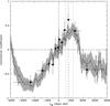 |
Fig. 9 Cross-correlation function of the BAL EW with the NAL EW variability. Both the ICCF (solid line) and the ZDCF computed with 20 points per bin (black dots) are shown with their respective 1σ errors. The ZDCF lag (dashed line) is indicated along with its uncertainty at 68% probability (dotted lines). |
4.2. The NAL variability
At variance with the BAL behaviour, in Paper I and Saturni et al. (2014) the “red NAL” did not appear to show variations related to the strong continuum variation at MJD ~ 55 000. We argued that this could have been caused by a delayed variation in the ionisation state of the NAL absorber, which was not yet seen in the LC, with respect to the continuum changes. We estimated a lower limit to this physical recombination time lag of ~200 rest-frame days, roughly corresponding to the time span between MJD ~ 55 000 and ~56 000 in our data (see Fig. 6). With this limit, we placed an upper limit of ne ≲ 2 × 104 cm-3 on the electron density of the absorber.
APM 08279+5255 relevant time lags.
With the update of the NAL EW time series presented in Fig. 6, a delayed rise seems to appear with respect to the continuum variation of ~0.4 mag after MJD ~ 55 000 with the NAL EW rising by ~0.2 dex between MJD ~ 56 000 and 57 000. At a glance, this would correspond to a rest-frame time lag of roughly 200 days. A measurement of this delay can provide a more robust estimate of the NAL electron density instead of the upper limit of Paper I.
We therefore compute the CCFs between the NAL EW and continuum variability. Both the ICCF and ZDCF are shown in the right panel of Fig. 8. At variance with the BAL case, here the correlation peak appears at different lags for ICCF ( days in the observer frame) and ZDCF (
 days), and both peaks are marginally significant at 2σ level (N = 19, r = 0.60, P( >r,N) = 0.01 for the ICCF; N = 15, r = 0.65, P( >r,N) = 0.01 for the ZDCF). Also, a visual inspection of Fig. 6 shows that the identification of the main CCF peaks is not straightforward.
However, in Paper I we suggested that the absorption variability occurs in response to the variations in the true C IV ionising continuum at ~200 Å, which is not observed. The BAL variability is assumed to trace this ionising continuum with no or very small recombination lag because of a high electron density of the absorbing wind. Therefore, we assume the BAL EW time series as a proxy of the ionising continuum variability, and compute ICCF and ZDCF with the NAL EWs. The result is shown in Fig. 9; a single peak arises at  days in the observer frame for the ICCF and at
  days for the ZDCF with a significance at more than 2σ level in both cases (N = 26, r = 0.43, P( >r,N) = 0.02 for the ICCF; N = 20, r = 0.62, P( >r,N) = 3 × 10⁻³ for the ZDCF). This favours the correlation between the continuum flux decrease beginning at MJD ~ 55 000 and the NAL EW rise after MJD ~ 56 000. Moreover, it suggests at the same time that the BAL variability is in fact a better proxy of the ionising continuum variations than the R-band continuum.
5. Discussion
We have obtained several time lags linking the variability of emission and absorption lines to that of the driving continuum emission owing to our long-time spectro-photometric monitoring of the high-z bright quasar APM 08279+5255. In this way, we are able to probe (i) the region of the ionised gas clouds producing the emission lines; and (ii) the regions where the high-velocity outflows responsible for broad absorption in quasar spectra originate. In Table 1, we summarise all these time lags together, giving them both in the observer frame and in the rest frame for z = 3.911.
In this section, we discuss what can be inferred about the relevant physical parameters of these regions. From the Si IV and C IV emission-line lags, we can estimate the black hole mass of APM 08279+5255 with some assumptions on the BLR shape and inclination (which are summarised into the form factor f). From the C IV NAL recombination lag with respect to the ionising continuum at ~200 Å, we can obtain information about the electron density and the distance of the absorbing gas from the central engine.
5.1. Si IV and C IV BLR stratification
Since the time lags obtained for Si IV and for C IV are equal within errors, this means that the respective BLRs must be approximately located at the same distance from the central black hole. How does this compare with the BLR size ratio found in low-luminosity AGNs? To explore this point, we collected from the literature all the objects with RM time lags of both Si IV and C IV. These objects are the Seyfert galaxies NGC 3783, NGC 5548, and NGC 7469 (Peterson et al. 2004).
In Fig. 10 we show such collection of rest-frame time lags from Si IV as a function of those from C IV, and perform a logarithmic bisector fit to the data to quantify the average size difference between Si IV and C IV BLRs from Seyfert galaxies to quasars, spanning three orders of magnitude of BLR size. Allowing both slope and intercept to vary, the fit indicates a possible increase of the time lag ratio, and hence of the BLR size ratio with a power-law behaviour with logarithmic slope 1.10 ± 0.03. For comparison, a fit with a unitary slope is also shown in Fig. 10, corresponding to an average ratio  . This result is dominated by the Seyfert galaxies, whose average ratio is
 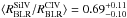 .
.
5.2. The size-luminosity relation for the C IV BLR
Our result for APM 08279+5255 allows us to extend the size-luminosity relation for the C IV emitting region up to ~1048 erg s-1 in monochromatic luminosity at 1350 Å λLλ(1350). In Fig. 11 we collect all the available data for the size of the C IV emitting region in AGNs as a function of their λLλ(1350), where we add our point for APM 08279+5255 to spectroscopic RM measurements (Peterson et al. 2004, 2005; Metzroth et al. 2006; Kaspi et al. 2007; Perna et al. 2014; Trevese et al. 2014). Also, we add the point for the quasar MACHO 13.6805.324 obtained with photometric RM by Chelouche et al. (2012) and the point for the gravitationally lensed quasar QSO 2237+0305 obtained through microlensing by Sluse et al. (2011).
We fit a power-law relation  to this data set with a method that takes the uncertainties in both variables and the intrinsic scatter of points into account. We run a high number of bisector fits (Akritas & Bershady 1996) on data sets in which each original point is replaced by casting a pair of substituting values within the associated error box; these values are weighted by an asymmetric distribution function, which are represented by two demi-Gaussian distributions with different standard deviations, corresponding to the asymmetric uncertainties. The best-fit relation obtained with 104 runs is
 ![\begin{equation} \label{rlciveq} \log{R_{\rm BLR}} = (0.9 \pm 0.7) + (0.54 \pm 0.02) \log{\left[\frac{\lambda L_\lambda (1350)}{10^{44}\mbox{ erg s}^{-1}} \right]}\cdot \end{equation}](/articles/aa/full_html/2016/03/aa27152-15/aa27152-15-eq143.png) (5)With respect to previous relations (Peterson et al. 2005; Kaspi et al. 2007), having added objects with uncertain luminosities to the fit gives a large error in the intercept. In the two cases of the quasars PG 1247+267 and APM 08279+5255, this is due to the unknown lens magnification factor μ. In fact, as described in Trevese et al. (2014), the first object has relatively small emission-line widths with respect to its luminosity, an Eddington ration of ~10, and a significant deviation from the αOX – L2500 relation (Shemmer et al. 2014). An invisible gravitational lens with μ ≈ 10 could explain all the anomalies described in Trevese et al. (2014). For APM 08279+5255, instead, the fact that the lensing galaxy is not visible (Lewis et al. 2002) leads to very model-dependent estimates of the magnification factor. Currently, μ ranges between ~100 (Egami et al. 2000) and ~4 (Riechers et al. 2009) for APM 08279+5255. Therefore, to provide a rough indication of the global uncertainty due to both the statistical errors and the ignorance of the lens magnification, we adopt as uncertainty in the quasar luminosity the whole range of plausible λLλ(1350) between μ = 4 and 100 for APM 08279+5255, and the range between μ = 1 (i.e. no magnification) and 10 for PG 1247+267.
(5)With respect to previous relations (Peterson et al. 2005; Kaspi et al. 2007), having added objects with uncertain luminosities to the fit gives a large error in the intercept. In the two cases of the quasars PG 1247+267 and APM 08279+5255, this is due to the unknown lens magnification factor μ. In fact, as described in Trevese et al. (2014), the first object has relatively small emission-line widths with respect to its luminosity, an Eddington ration of ~10, and a significant deviation from the αOX – L2500 relation (Shemmer et al. 2014). An invisible gravitational lens with μ ≈ 10 could explain all the anomalies described in Trevese et al. (2014). For APM 08279+5255, instead, the fact that the lensing galaxy is not visible (Lewis et al. 2002) leads to very model-dependent estimates of the magnification factor. Currently, μ ranges between ~100 (Egami et al. 2000) and ~4 (Riechers et al. 2009) for APM 08279+5255. Therefore, to provide a rough indication of the global uncertainty due to both the statistical errors and the ignorance of the lens magnification, we adopt as uncertainty in the quasar luminosity the whole range of plausible λLλ(1350) between μ = 4 and 100 for APM 08279+5255, and the range between μ = 1 (i.e. no magnification) and 10 for PG 1247+267.
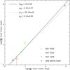 |
Fig. 10 Rest-frame Si IV time lags as a function of C IV lags. All the available data from the literature are shown, together with our measurements from the RM of APM 08279+5255 (legend is on the plot). We performed a free linear fit in the logarithmic space (solid line) and a linear fit with logarithmic slope fixed to unity (dotted line) for the whole data set. Fit coefficients are indicated in the plot with their 1σ errors. |
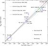 |
Fig. 11 Size-luminosity relation for C IV BLR. Together with APM 08279+5255, all the objects with measurements of C IV BLR size and monochromatic luminosity at 1350 Å available in the literature have been included in this plot: NGC 4395, NGC 7469, NGC 3783, NGC 5548, and 3C 390.3 from Peterson et al. (2004, 2005), NGC 4151 from Metzroth et al. (2006), QSO 2237+0305 from Sluse et al. (2011), MACHO 13.6805.324 from Chelouche et al. (2012), S5 0836+71 from Kaspi et al. (2007), and PG 1247+267 from Perna et al. (2014), Trevese et al. (2014). Colour and symbol codes are explained in the plot. For comparison with our fit, we also report the fits performed by Peterson et al. (2005, 2006) and Kaspi et al. (2007) (see legend in the plot). |
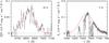 |
Fig. 12 Left panel: continuum-subtracted rms spectrum of APM 08279+5255 Si IV emission line from our RM monitoring. Right panel: continuum-subtracted HST spectrum of the C IV emission line. In both panels, errors on the flux level (grey bars) and best-fit Gaussians (red curves) are shown. For Si IV, the major deviations from the best-fit curve are the residuals of intrinsic narrow absorptions superimposed to the emission line, as can be seen from the analysis by Srianand & Petitjean (2000) and Ellison et al. (2004). |
5.3. APM 08279+5255 black hole mass estimates
We follow the approach of Trevese et al. (2014) to give a direct estimate of the black hole mass of APM 08279+5255. Therefore, we first identify the velocity Δv appearing in Eq. (1) with the rms velocity dispersion along the line of sight σl. We then compute the uncertainty on σl for Si IV by applying the bootstrap method described in Peterson et al. (2004), obtaining  km s-1; the use of σl both avoids underestimates of Δv caused by narrow emission-line components and the effect of non-virial outflows varying on timescales longer than RM lags (e.g. Denney 2012).
Unfortunately, we cannot apply the same procedure to C IV, since its emission-line profile is heavily affected by absorption features that prevent us from computing a reliable rms spectrum in that region. Therefore, instead of using σl, for C IV we adopt the standard deviation of a Gaussian profile σg = 3200 ± 30 km s-1, as measured through the C IV emission profile fit performed on the high-resolution, dereddened HST/STIS spectrum of APM 08279+5255. Since the unabsorbed spectral intervals in this spectrum appear to be free of narrow components and outflows in emission, we can consider this a good equivalent estimate of the proper C IV rms σl. In Fig. 12, we show both the fit of C IV on the HST spectrum and a Gaussian fit of the rms Si IV, performed by only allowing the rms line amplitude to vary, setting the peak wavelength to λ1400 Å at z = 3.87 (Irwin et al. 1998; Downes et al. 1999), and the line width to the Si IV σl.
Finally, we multiply the posterior distributions of tlag for Si IV and C IV for the respective statistical distributions of Δv2 to obtain two posterior distributions of APM 08279+5255 virial products tlagΔv2, to be inserted in Eq. (1) to obtain the black hole mass MBH. We adopt as a form factor the value f = 5.5, obtained by Onken et al. (2004) through the calibration of the Hβ RM masses on the relation between black hole masses and stellar velocity dispersions in galaxy bulges (Ferrarese & Merritt 2000; Merritt & Ferrarese 2001b; Gültekin et al. 2009), which is appropriate for the definition of Δv = σl (not FWHM). Although more recent estimates provide different values for f (e.g. Pancoast et al. 2014 and refs. therein), we nonetheless choose this commonly used value for a direct comparison with the literature, following Trevese et al. (2014). Figure 13 shows such distributions, which give an identical result of 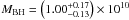 M⊙ as best estimate of the virial mass.
5.4. Estimate of the lens magnification
APM 08279+5255, a well-known gravitational lens, is the first confirmed case with an odd number of images of the lensed source and no observed trace of the lensing galaxy (Lewis et al. 2002). Therefore, the estimate of the lens magnification μ only relies on modelling the lensed quasar image from high-resolution optical/infrared imaging, and the values of μ are significantly discrepant when estimated from different lens models (Egami et al. 2000; Riechers et al. 2009). This primarily affects the single-epoch black hole mass estimates from mass-luminosity virial relationships, which can give differences in the value of MBH of up to one order of magnitude when adopting such magnifications.
Our direct RM measurement of the C IV RBLR for APM 08279+5255 allows us to invert the relation between the BLR size and UV luminosity, thus giving a model-independent estimate of μ that can discriminate between the competing models. We thus solve Eq. (3) of Kaspi et al. (2007) for λLλ(1350), which is not affected by our ignorance of APM 08279+5255 true luminosity, adopting our fiducial JAVELIN time lag for C IV of 901 days in the rest frame  (6)With a measured luminosity
  erg s-1 from our dereddened spectra, the lens magnification can be estimated by
  (7)This low magnification favours the lens model by Riechers et al. (2009) with respect to that by Egami et al. (2000), although it is affected by large errors as a result of the uncertainty on the BLR-luminosity relation.
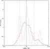 |
Fig. 13 Posterior distribution of APM 08279+5255 black hole mass from Si IV (blue solid histogram) and C IV (red dashed histogram) RM. The best estimate of the black hole mass (dot-dashed line) is indicated together with its confidence intervals at 68% probability (dotted lines). |
5.5. Black hole mass versus host-galaxy mass – an overmassive black hole for APM 08279+5255
Having measured the black hole mass of APM 08279+5255, we now address the question of how it compares with the mass of the host galaxy. From the known relation between black hole mass and host-galaxy bulge mass for nearby galaxies (Magorrian et al. 1998; Merritt & Ferrarese 2001a; Marconi & Hunt 2003; Häring & Rix 2004), the expected bulge mass Mbulge for APM 08279+5255 would be ~400 times MBH. From CO emission-line structure, Riechers et al. (2009) derived Mbulge = 3.0 × 10¹¹/μ M⊙, which corresponds to 7.5 × 10¹⁰ M⊙ for μ = 4. Using our RM measurement of MBH, this means that Mbulge = 7.5MBH for APM 08279+5255, which is slightly higher than Riechers et al. (2009) estimate but still more than 50 times lower than the value extrapolated from the local Mbulge−MBH ratio.
This revised result confirms the conclusions by Riechers et al. (2009), i.e. black hole mass assembly had already ended at very early cosmic times within a galaxy that is still forming the largest part of its stars. A handful of other objects presenting a similar MBH/Mbulge ~ 0.1 are known so far (Walter et al. 2004; Riechers et al. 2008a,b), and APM 08279+5255 is the first with a direct estimate of its MBH. High MBH/Mbulge ratios may be common at high redshift with a non-evolving black hole-to-total stellar mass ratio (MBH/M∗) as stars later settle into galaxy bulges and a MBH/Mbulge ratio at z ~ 0 (e.g. Jahnke et al. 2009).
The value of M∗ for APM 08729+5255 is currently unknown; still, in the MBH−M∗ diagram (see Fig. 2 of Trakhtenbrot et al. 2015), APM 08279+5255 hosts one of the most massive black holes measured so far. Its MBH is in fact slightly higher than CID-947, a z ~ 3.3 quasar interpreted as a possible prototype of a class of objects with still largely incomplete star formation in the host galaxy (Trakhtenbrot et al. 2015).
5.6. Physics and location of the C IV absorbing gas
We argued in Paper I that the most plausible mechanism for absorption variability in APM 08279+5255 is a change in the photo-ionisation state of the gas driven by the variability of the ionising continuum. Within this framework, the increase in the absorption EWs after the flux drop at MJD ~ 55 000 is due to an equivalent increase in the density of C IV ions through the recombination process C4 + → C3+. The timescales, obtained through the CCF between the absorption and continuum variability, measure the delay between a variation in the quasar radiation field and the corresponding variation in the density of the absorbing ions, through which we can infer the density of the absorbing gas and thus its distance, or at least a lower limit on its distance, from the central engine.
Since the change in the BAL EW is simultaneous with the R-band strong continuum variation, the time lag obtained for the main C IV broad absorption features is compatible with zero. Thus, we cannot establish a significant lower limit on the electron density of the BAL wind.
Conversely, the observed lag in the NAL EW variability can give an estimate of the density of the absorbing clouds ne. Assuming αrec = 2.8 × 10⁻¹² cm3 s-1 (Arnaud & Rothenflug 1985) as the recombination coefficient of C4+ atoms, we compute the value of ne as follows:  (8)assuming the ZDCF lag computed with respect to the BAL variability (see Sect. 4.2) as an estimate of the NAL recombination time lag.
A rough estimate of the distance of the NAL gas from the continuum source may be obtained through the knowledge of the ionisation parameter U of APM 08279+5255, which is linked to the distance from the ionising source and to its luminosity by (e.g. Peterson 1997)  (9)We can derive r as
  (10)where we adopt U ~ 10-2 from Srianand & Petitjean (2000). In order to estimate Lν over the range of (unobserved) ionising energies, we follow the procedure of Grier et al. (2015), calibrating the synthetic quasar spectral energy distribution (SED) of Dunn et al. (2010) to APM 08279+5255 bolometric luminosity Lbol ~ 4.5 × 1048 erg s-1. This luminosity is inferred from the observed flux density at 3000 Å of the optical/IR spectrum of APM 08279+5255 taken at the Telescopio Nazionale Galileo (La Palma, Canarian Islands; Saturni et al., in prep.) with a bolometric correction factor of 5 (Richards et al. 2006) and the lens magnification μ = 4 of Riechers et al. (2009); with this normalisation, we compute
  s-1 for energies of up to 50 keV. Substituting these quantities in Eq. (10), we finally obtain rNAL ≈ 9.6 kpc, which is compatible with a location of the NAL absorbers in the body of APM 08279+5255 host galaxy.
6. Conclusions
The long monitoring of APM 08279+5255 obtained by combining our observational campaign with literature data, including a total sample of 138 photometric R-band points and 30 spectra (plus five from the literature used for the study of the C IV absorption variability) spanning ~16 years in the observer frame (~3.5 years in the rest frame), allowed us to perform the RM of this quasar. The resulting rest-frame time lag is ~900 days in the rest frame for both Si IV and C IV. We summarise the conclusions that derive from this result as follows:
-
1.
We find
 for APM 08279+5255. This ratio is only marginally consistent with the average value found for Seyfert galaxies (
 ), thus possibly indicating a slight increase of
  from Seyferts to quasars.
 -
2.
We update the distance-luminosity relation for quasars obtained through C IV lags (Peterson et al. 2005; Kaspi et al. 2007) and compute a black hole mass of ~1010 M⊙ for APM 08279+5255.
-
3.
With our direct time lag measurement, we can invert the distance-luminosity relation for C IV of Kaspi et al. (2007) to obtain an estimate of APM 08279+5255 lens magnification, which is so far uncertain between 100 (Egami et al. 2000) and 4 (Riechers et al. 2009), depending on the model of the lensing galaxy shape, size, and positioning. This provides an estimate of
 , which is consistent at 1σ level with the model of Riechers et al. (2009) and disfavours the model of Egami et al. (2000).
 -
4.
We revise the MBH/Mbulge ratio presented by Riechers et al. (2009), confirming that APM 08279+5255 has an oversized black hole with respect to its host-galaxy bulge (Walter et al. 2004; Riechers et al. 2008a,b). A future measurement of its host-galaxy stellar mass would be extremely important to establish whether the APM 08279+5255 host galaxy has an under-developed stellar component in analogy with the case of CID-947 (Trakhtenbrot et al. 2015).
We also update the study on the C IV absorption variability already presented in Paper I and Saturni et al. (2014) and further strengthen the hypothesis of BAL variations driven by changes in the C IV ionising continuum at ~200 Å. At variance with the BAL components, the narrow absorption system redwards of the C IV λ1549 emission exhibits a variation delayed by ~160 days in the rest frame with respect to the ionising continuum. Under the assumption that this lag is due to C+ 4 → C+3 recombination, we estimate a distance of the NAL gas from the central engine that is consistent with galactic sizes.
Available at http://www.astronomy.ohio-state.edu/~yingzu/codes.html
Both scripts are available at http://wwo.weizmann.ac.il/weizsites/tal/research/software/
Acknowledgments
We thank our anonymous referee for their helpful comments. We are also grateful to Ying Zu (McWilliams Center for Cosmology, Carnegie Mellon University) for the useful discussion about the use of JAVELIN. We acknowledge funding from PRIN/MIUR-2010 award 2010NHBSBE. M.D. acknowledges PRIN INAF 2011 funding. This research is based on observations collected at the Copernico telescope (Asiago, Italy) of the INAF-Osservatorio Astronomico di Padova, and at the Cassini Telescope (Loiano, Italy) of the INAF-Osservatorio Astronomico di Bologna.
References
- Akritas, M. G., & Bershady, M. A. 1996, ApJ, 470, 706 [NASA ADS] [CrossRef] [Google Scholar]
- Alexander, T. 1997, in Astronomical Time Series, eds. D. Maoz, A. Sternberg, & E. M. Leibowitz, Astrophys. Space Sci. Libr., 218, 163 [Google Scholar]
- Alexander, T. 2013, ArXiv e-prints [arXiv:1302.1508] [Google Scholar]
- Arnaud, M., & Rothenflug, R. 1985, A&AS, 60, 425 [NASA ADS] [Google Scholar]
- Barlow, T. A. 1993, Ph.D. Thesis, California University [Google Scholar]
- Barlow, T. A., Junkkarinen, V. T., Burbidge, E. M., et al. 1992, ApJ, 397, 81 [NASA ADS] [CrossRef] [Google Scholar]
- Bevington, P. R. 1969, Data reduction and error analysis for the physical sciences (New York: McGraw-Hill) [Google Scholar]
- Brandt, W. N., Filiz Ak, N., Hall, P. B., Schneider, D. P., & SDSS-III BAL Variability Team. 2014, in AAS Meet. Abstracts, 223, 126.01 [Google Scholar]
- Capellupo, D. M., Hamann, F., Shields, J. C., Rodríguez Hidalgo, P., & Barlow, T. A. 2011, MNRAS, 413, 908 [NASA ADS] [CrossRef] [Google Scholar]
- Capellupo, D. M., Hamann, F., Shields, J. C., Rodríguez Hidalgo, P., & Barlow, T. A. 2012, MNRAS, 422, 3249 [NASA ADS] [CrossRef] [Google Scholar]
- Capellupo, D. M., Hamann, F., Shields, J. C., Halpern, J. P., & Barlow, T. A. 2013, MNRAS, 429, 1872 [NASA ADS] [CrossRef] [Google Scholar]
- Cattaneo, A., Faber, S. M., Binney, J., et al. 2009, Nature, 460, 213 [NASA ADS] [CrossRef] [PubMed] [Google Scholar]
- Chelouche, D., Daniel, E., & Kaspi, S. 2012, ApJ, 750, L43 [NASA ADS] [CrossRef] [Google Scholar]
- Denney, K. D. 2012, ApJ, 759, 44 [NASA ADS] [CrossRef] [Google Scholar]
- Downes, D., Neri, R., Wiklind, T., Wilner, D. J., & Shaver, P. A. 1999, ApJ, 513, L1 [NASA ADS] [CrossRef] [Google Scholar]
- Drake, A. J., Djorgovski, S. G., Mahabal, A., et al. 2009, ApJ, 696, 870 [NASA ADS] [CrossRef] [MathSciNet] [Google Scholar]
- Dunn, J. P., Bautista, M., Arav, N., et al. 2010, ApJ, 709, 611 [NASA ADS] [CrossRef] [Google Scholar]
- Edelson, R. A., & Krolik, J. H. 1988, ApJ, 333, 646 [NASA ADS] [CrossRef] [Google Scholar]
- Egami, E., Neugebauer, G., Soifer, B. T., et al. 2000, ApJ, 535, 561 [NASA ADS] [CrossRef] [Google Scholar]
- Ellison, S. L., Lewis, G. F., Pettini, M., et al. 1999, PASP, 111, 946 [NASA ADS] [CrossRef] [Google Scholar]
- Ellison, S. L., Ibata, R., Pettini, M., et al. 2004, A&A, 414, 79 [NASA ADS] [CrossRef] [EDP Sciences] [Google Scholar]
- Elvis, M. 2000, ApJ, 545, 63 [NASA ADS] [CrossRef] [Google Scholar]
- Ferrarese, L., & Merritt, D. 2000, ApJ, 539, L9 [NASA ADS] [CrossRef] [Google Scholar]
- FilizAk, N., Brandt, W. N., Hall, P. B., et al. 2013, ApJ, 777, 168 [NASA ADS] [CrossRef] [Google Scholar]
- Gaskell, C. M., & Peterson, B. M. 1987, ApJS, 65, 1 [NASA ADS] [CrossRef] [Google Scholar]
- Gibson, R. R., Brandt, W. N., Schneider, D. P., & Gallagher, S. C. 2008, ApJ, 675, 985 [NASA ADS] [CrossRef] [Google Scholar]
- Grier, C. J., Hall, P. B., Brandt, W. N., et al. 2015, ApJ, 806, 111 [NASA ADS] [CrossRef] [Google Scholar]
- Gültekin, K., Richstone, D. O., Gebhardt, K., et al. 2009, ApJ, 698, 198 [NASA ADS] [CrossRef] [Google Scholar]
- Hall, P. B., Anosov, K., White, R. L., et al. 2011, MNRAS, 411, 2653 [NASA ADS] [CrossRef] [Google Scholar]
- Häring, N., & Rix, H.-W. 2004, ApJ, 604, L89 [NASA ADS] [CrossRef] [Google Scholar]
- Hines, D. C., Schmidt, G. D., & Smith, P. S. 1999, ApJ, 514, L91 [NASA ADS] [CrossRef] [Google Scholar]
- Irwin, M. J., Ibata, R. A., Lewis, G. F., & Totten, E. J. 1998, ApJ, 505, 529 [NASA ADS] [CrossRef] [Google Scholar]
- Jahnke, K., Bongiorno, A., Brusa, M., et al. 2009, ApJ, 706, L215 [NASA ADS] [CrossRef] [Google Scholar]
- Kaspi, S., Smith, P. S., Netzer, H., et al. 2000, ApJ, 533, 631 [NASA ADS] [CrossRef] [Google Scholar]
- Kaspi, S., Brandt, W. N., Maoz, D., et al. 2007, ApJ, 659, 997 [NASA ADS] [CrossRef] [Google Scholar]
- Kelly, B. C., Bechtold, J., & Siemiginowska, A. 2009, ApJ, 698, 895 [Google Scholar]
- Kozłowski, S., Kochanek, C. S., Udalski, A., et al. 2010, ApJ, 708, 927 [NASA ADS] [CrossRef] [Google Scholar]
- Krongold, Y., Binette, L., & Hernández-Ibarra, F. 2010, ApJ, 724, L203 [NASA ADS] [CrossRef] [Google Scholar]
- Lewis, G. F., Robb, R. M., & Ibata, R. A. 1999, PASP, 111, 1503 [NASA ADS] [CrossRef] [Google Scholar]
- Lewis, G. F., Ibata, R. A., Ellison, S. L., et al. 2002, MNRAS, 334, L7 [NASA ADS] [CrossRef] [Google Scholar]
- Lundgren, B. F., Wilhite, B. C., Brunner, R. J., et al. 2007, ApJ, 656, 73 [NASA ADS] [CrossRef] [Google Scholar]
- Lynds, C. R. 1967, ApJ, 147, 396 [NASA ADS] [CrossRef] [Google Scholar]
- MacLeod, C. L., Ivezić, Ž., Kochanek, C. S., et al. 2010, ApJ, 721, 1014 [NASA ADS] [CrossRef] [Google Scholar]
- Magorrian, J., Tremaine, S., Richstone, D., et al. 1998, AJ, 115, 2285 [NASA ADS] [CrossRef] [Google Scholar]
- Marconi, A., & Hunt, L. K. 2003, ApJ, 589, L21 [NASA ADS] [CrossRef] [Google Scholar]
- McLure, R. J., & Dunlop, J. S. 2004, MNRAS, 352, 1390 [NASA ADS] [CrossRef] [Google Scholar]
- Merritt, D., & Ferrarese, L. 2001a, MNRAS, 320, L30 [NASA ADS] [CrossRef] [Google Scholar]
- Merritt, D., & Ferrarese, L. 2001b, ApJ, 547, 140 [NASA ADS] [CrossRef] [Google Scholar]
- Metzroth, K. G., Onken, C. A., & Peterson, B. M. 2006, ApJ, 647, 901 [NASA ADS] [CrossRef] [Google Scholar]
- Netzer, H. 2003, ApJ, 583, L5 [NASA ADS] [CrossRef] [Google Scholar]
- Onken, C. A., Ferrarese, L., Merritt, D., et al. 2004, ApJ, 615, 645 [NASA ADS] [CrossRef] [Google Scholar]
- Pancoast, A., Brewer, B. J., Treu, T., et al. 2014, MNRAS, 445, 3073 [NASA ADS] [CrossRef] [Google Scholar]
- Pei, Y. C. 1992, ApJ, 395, 130 [NASA ADS] [CrossRef] [Google Scholar]
- Perna, M., Trevese, D., Vagnetti, F., & Saturni, F. G. 2014, Adv. Space Res., 54, 1429 [NASA ADS] [CrossRef] [Google Scholar]
- Peterson, B. M. 1993, PASP, 105, 247 [NASA ADS] [CrossRef] [Google Scholar]
- Peterson, B. M. 1997, in An Introduction to Active Galactic Nuclei (Cambridge, New York: Cambridge University Press), 238 [Google Scholar]
- Peterson, B. M., Wanders, I., Horne, K., et al. 1998, PASP, 110, 660 [NASA ADS] [CrossRef] [Google Scholar]
- Peterson, B. M., Ferrarese, L., Gilbert, K. M., et al. 2004, ApJ, 613, 682 [NASA ADS] [CrossRef] [Google Scholar]
- Peterson, B. M., Bentz, M. C., Desroches, L.-B., et al. 2005, ApJ, 632, 799 [NASA ADS] [CrossRef] [Google Scholar]
- Peterson, B. M., Bentz, M. C., Desroches, L.-B., et al. 2006, ApJ, 641, 638 [NASA ADS] [CrossRef] [Google Scholar]
- Petitjean, P., Aracil, B., Srianand, R., & Ibata, R. 2000, A&A, 359, 457 [NASA ADS] [Google Scholar]
- Press, W. H., Rybicki, G. B., & Hewitt, J. N. 1992, ApJ, 385, 416 [NASA ADS] [CrossRef] [EDP Sciences] [Google Scholar]
- Richards, G. T., Lacy, M., Storrie-Lombardi, L. J., et al. 2006, ApJS, 166, 470 [NASA ADS] [CrossRef] [Google Scholar]
- Riechers, D. A., Walter, F., Brewer, B. J., et al. 2008a, ApJ, 686, 851 [NASA ADS] [CrossRef] [Google Scholar]
- Riechers, D. A., Walter, F., Carilli, C. L., Bertoldi, F., & Momjian, E. 2008b, ApJ, 686, L9 [NASA ADS] [CrossRef] [Google Scholar]
- Riechers, D. A., Walter, F., Carilli, C. L., & Lewis, G. F. 2009, ApJ, 690, 463 [NASA ADS] [CrossRef] [Google Scholar]
- Röser, S., Demleitner, M., & Schilbach, E. 2010, AJ, 139, 2440 [NASA ADS] [CrossRef] [Google Scholar]
- Rybicki, G. B., & Kleyna, J. T. 1994, in Reverberation Mapping of the Broad-Line Region in Active Galactic Nuclei, eds. P. M. Gondhalekar, K. Horne, & B. M. Peterson, ASP Conf. Ser., 69, 85 [Google Scholar]
- Rybicki, G. B., & Press, W. H. 1992, ApJ, 398, 169 [NASA ADS] [CrossRef] [Google Scholar]
- Salpeter, E. E. 1964, ApJ, 140, 796 [CrossRef] [Google Scholar]
- Saturni, F. G., Trevese, D., Vagnetti, F., & Perna, M. 2014, Adv. Space Res., 54, 1434 [NASA ADS] [CrossRef] [Google Scholar]
- Shemmer, O., Brandt, W. N., Paolillo, M., et al. 2014, ApJ, 783, 116 [NASA ADS] [CrossRef] [Google Scholar]
- Shen, Y., Richards, G. T., Strauss, M. A., et al. 2011, ApJS, 194, 45 [NASA ADS] [CrossRef] [Google Scholar]
- Shen, Y., Brandt, W. N., Dawson, K. S., et al. 2015, ApJS, 216, 4 [NASA ADS] [CrossRef] [Google Scholar]
- Sluse, D., Schmidt, R., Courbin, F., et al. 2011, A&A, 528, A100 [NASA ADS] [CrossRef] [EDP Sciences] [Google Scholar]
- Srianand, R., & Petitjean, P. 2000, A&A, 357, 414 [NASA ADS] [Google Scholar]
- Trakhtenbrot, B., Urry, C. M., Civano, F., et al. 2015, Science, 349, 168 [NASA ADS] [CrossRef] [Google Scholar]
- Trevese, D., Paris, D., Stirpe, G. M., Vagnetti, F., & Zitelli, V. 2007, A&A, 470, 491 [NASA ADS] [CrossRef] [EDP Sciences] [Google Scholar]
- Trevese, D., Saturni, F. G., Vagnetti, F., et al. 2013, A&A, 557, A91 [NASA ADS] [CrossRef] [EDP Sciences] [Google Scholar]
- Trevese, D., Perna, M., Vagnetti, F., Saturni, F. G., & Dadina, M. 2014, ApJ, 795, 164 [NASA ADS] [CrossRef] [Google Scholar]
- Turnshek, D. A. 1988, in QSO Absorption Lines: Probing the Universe, eds. J. C. Blades, D. A. Turnshek, & C. A. Norman, 17 [Google Scholar]
- Urry, C. M., & Padovani, P. 1995, PASP, 107, 803 [NASA ADS] [CrossRef] [Google Scholar]
- Vestergaard, M., & Peterson, B. M. 2006, ApJ, 641, 689 [NASA ADS] [CrossRef] [Google Scholar]
- Walter, F., Carilli, C., Bertoldi, F., et al. 2004, ApJ, 615, L17 [CrossRef] [Google Scholar]
- Wandel, A., Peterson, B. M., & Malkan, M. A. 1999, ApJ, 526, 579 [NASA ADS] [CrossRef] [Google Scholar]
- Welsh, W. F. 1999, PASP, 111, 1347 [NASA ADS] [CrossRef] [Google Scholar]
- Weymann, R., & Foltz, C. 1983, in Liège Int. Astrophys. Colloq. 24, ed. J.-P. Swings, 538 [Google Scholar]
- White, R. J., & Peterson, B. M. 1994, PASP, 106, 879 [NASA ADS] [CrossRef] [Google Scholar]
- Zel’dovich, Y. B., & Novikov, I. D. 1965, Soviet Physics Doklady, 9, 834 [Google Scholar]
- Zu, Y., Kochanek, C. S., & Peterson, B. M. 2011, ApJ, 735, 80 [NASA ADS] [CrossRef] [Google Scholar]
- Zu, Y., Kochanek, C. S., Kozłowski, S., & Udalski, A. 2013, ApJ, 765, 106 [NASA ADS] [CrossRef] [Google Scholar]
Appendix A: Additional table
APM 08279+5255 continuum and emission-line fluxes.
All Tables
All Figures
|
Fig. 1 Dereddened spectrum of APM 08279+5255 taken at MJD = 52 695 at the 1.82 m Copernico telescope (Asiago, Italy). Superimposed on the spectrum (black solid line), a power-law continuum (blue dot-dashed line), a Gaussian fit of the C IV emission line (green dashed line), and the combination of these two components into a single pseudo-continuum (red solid line) are shown. The dotted line indicates the flux zero level. The major absorption features are denoted with the identifiers used in the text (see Sect. 4) and ticks. The positions of the Lyman limit at λ912 Å in the rest frame and the major emission lines are also indicated. |
| In the text | |
|
Fig. 2 Upper panel: R-band continuum light curve of APM 08279+5255. The Lewis et al. (1999) photometric campaign (red triangles), the Asiago and Loiano (Trevese et al. 2007, 2013, 2014) RM campaign (green dots), and the rescaled V-band Catalina photometry (blue crosses) are all included. Superimposed on the data, the best-fit DRW variability model computed by JAVELIN (Zu et al. 2011) is shown (black solid line) delimited by its error boundaries at 68% probability (black dashed lines). Middle panel: Si IV light curve. Lower panel: C IV light curve. |
| In the text | |
|
Fig. 3 Posterior distributions of the Si IV (blue solid histogram) and C IV (red dashed histogram) RM time lags computed with JAVELIN. The time-lag mean values (blue point and red square) for each distribution are shown together with their corresponding confidence intervals at 68% (colour and line-type codes as per the histograms) and at 95% probability (dotted error bars). |
| In the text | |
|
Fig. 4 APM 08279+5255 light curve composed with the continuum (black dots) and emission-line fluxes, which are scaled in intensity and shifted in time of their JAVELIN lags of 837 and 901 rest-frame days, respectively, to mimic the original continuum light curve that is reverberated by the quasar BLR. Upper panel: continuum and Si IV (red triangles). Lower panel: continuum and C IV (blue crosses). In both panels, a DRW continuum, fitted by JAVELIN to the data with the damping timescale τd blocked to that of the continuum fit, is shown superimposed to the light curve (solid line) along with its 1σ error band (dashed lines). |
| In the text | |
|
Fig. 5 Upper panel: ICCF (solid line) with its 1σ error (grey area) and ZDCF (black points) for the continuum and the Si IV emission line. Lower panel: same as in the upper panel, but for the continuum and the C IV emission line. The ZDCF is computed over 15 uncorrelated points per bin, and finds a simultaneous peak for the two emission features at |
| In the text | |
|
Fig. 6 Upper panel: updated time series of APM 08279+5255 R-band differential magnitude with 1σ errors, adding all the photometric data available in literature (same colour code than in the upper panel of Fig. 2). Middle panel: BAL EWs computed for all the existing APM 08279+5255 spectra with 1σ errors. Lower panel: NAL EWs computed for all the existing APM 08279+5255 spectra with 1σ errors. In both middle and lower panels, Irwin et al. (1998; red triangle), Ellison et al. (1999; green cross), Hines et al. (1999; blue circle), Lewis et al. (2002; cyan square) and Saturni et al. (2015; yellow star) spectra are all included along with the Asiago and Loiano spectra (magenta dots). |
| In the text | |
|
Fig. 7 EWs of the two C IV BAL troughs of APM 08279+5255, plotted one versus the other (black points). The red arrows connect consecutive epochs of EW pairs. The two correlation fits of BAL1 versus BAL2 and vice versa are shown (solid lines) along with the corresponding bisector fit ( dot-dashed line). Slope mbis and intercept qbis of such fit, correlation coefficient r, and corresponding null-hypothesis probability p( >r) are reported. The cross in the lower right corner represents the mean error on the data set in each direction. |
| In the text | |
|
Fig. 8 Left panel: cross-correlation function of the R-band magnitudes with the total C IV BAL EW tracing the continuum. Right panel: cross-correlation function of the R-band magnitudes with the total C IV “red” NAL EW. In both panels, both the ICCF (black solid line) with 1σ errors in the y direction (grey bars), and ZDCF computed with 15 points per bin (black points) with 1σ errors in both x and y directions, are shown. The dashed vertical lines indicate the delays of the most prominent peaks enclosed by their uncertainties at 68% probability (dotted lines), which are also numerically reported. |
| In the text | |
|
Fig. 9 Cross-correlation function of the BAL EW with the NAL EW variability. Both the ICCF (solid line) and the ZDCF computed with 20 points per bin (black dots) are shown with their respective 1σ errors. The ZDCF lag (dashed line) is indicated along with its uncertainty at 68% probability (dotted lines). |
| In the text | |
|
Fig. 10 Rest-frame Si IV time lags as a function of C IV lags. All the available data from the literature are shown, together with our measurements from the RM of APM 08279+5255 (legend is on the plot). We performed a free linear fit in the logarithmic space (solid line) and a linear fit with logarithmic slope fixed to unity (dotted line) for the whole data set. Fit coefficients are indicated in the plot with their 1σ errors. |
| In the text | |
|
Fig. 11 Size-luminosity relation for C IV BLR. Together with APM 08279+5255, all the objects with measurements of C IV BLR size and monochromatic luminosity at 1350 Å available in the literature have been included in this plot: NGC 4395, NGC 7469, NGC 3783, NGC 5548, and 3C 390.3 from Peterson et al. (2004, 2005), NGC 4151 from Metzroth et al. (2006), QSO 2237+0305 from Sluse et al. (2011), MACHO 13.6805.324 from Chelouche et al. (2012), S5 0836+71 from Kaspi et al. (2007), and PG 1247+267 from Perna et al. (2014), Trevese et al. (2014). Colour and symbol codes are explained in the plot. For comparison with our fit, we also report the fits performed by Peterson et al. (2005, 2006) and Kaspi et al. (2007) (see legend in the plot). |
| In the text | |
|
Fig. 12 Left panel: continuum-subtracted rms spectrum of APM 08279+5255 Si IV emission line from our RM monitoring. Right panel: continuum-subtracted HST spectrum of the C IV emission line. In both panels, errors on the flux level (grey bars) and best-fit Gaussians (red curves) are shown. For Si IV, the major deviations from the best-fit curve are the residuals of intrinsic narrow absorptions superimposed to the emission line, as can be seen from the analysis by Srianand & Petitjean (2000) and Ellison et al. (2004). |
| In the text | |
|
Fig. 13 Posterior distribution of APM 08279+5255 black hole mass from Si IV (blue solid histogram) and C IV (red dashed histogram) RM. The best estimate of the black hole mass (dot-dashed line) is indicated together with its confidence intervals at 68% probability (dotted lines). |
| In the text | |
Current usage metrics show cumulative count of Article Views (full-text article views including HTML views, PDF and ePub downloads, according to the available data) and Abstracts Views on Vision4Press platform.
Data correspond to usage on the plateform after 2015. The current usage metrics is available 48-96 hours after online publication and is updated daily on week days.
Initial download of the metrics may take a while.