| Issue |
A&A
Volume 584, December 2015
|
|
|---|---|---|
| Article Number | A4 | |
| Number of page(s) | 25 | |
| Section | Interstellar and circumstellar matter | |
| DOI | https://doi.org/10.1051/0004-6361/201526239 | |
| Published online | 13 November 2015 | |
From forced collapse to H ii region expansion in Mon R2: Envelope density structure and age determination with Herschel⋆,⋆⋆
1 Laboratoire AIM, CEA/IRFU CNRS/INSU Université Paris Diderot, CEA-Saclay, 91191 Gif-sur-Yvette Cedex, France
e-mail: pierre.didelon@cea.fr
2 Astrophysics Group, University of Exeter, EX4 4QL Exeter, UK
3 Maison de la Simulation, CEA-CNRS-INRIA-UPS-UVSQ, USR 3441, Centre d’étude de Saclay, 91191 Gif-Sur-Yvette, France
4 Joint ALMA Observatory, 3107 Alonso de Cordova, Vitacura, Santiago, Chile
5 Universität Heidelberg, Zentrum für Astronomie, Institut für Theoretische Astrophysik, Albert-Ueberle-Str. 2, 69120 Heidelberg, Germany
6 Department of Physics and Astronomy, West Virginia University, Morgantown, WV 26506, USA
7 Also Adjunct Astronomer at the National Radio Astronomy Observatory, PO Box 2, Green Bank, WV 24944, USA
8 Université de Bordeaux, OASU, Bordeaux, France
9 Cardiff University, Wales Cardiff CF103 XQ, UK
10 European Space Research and Technology Centre (ESA-ESTEC), Keplerlaan 1, PO Box 299, 2200 AG Noordwijk, The Netherlands
11 Cerro Calan, Observatorio Astronmico Nacional, Camino el Observatorio, 1515 Las Condes, Chile
12 Laboratoire d’Astrophysique de Marseille, CNRS/INSU–Université de Provence, 13388 Marseille Cedex 13, France
13 Queen Mary + Westf. College, Dept. of Physics, London E1 4NS, UK
14 CESR, 31028 Toulouse, France
15 INAF–Istituto di Astrofisica e Planetologia Spaziali, via Fosso del Cavaliere 100, 00133 Rome, Italy
16 National Research Council of Canada, Herzberg Institute of Astrophysics, 5071 West Saanich Rd., Victoria, BC, V9E 2E7, Canada
17 University of Victoria, Department of Physics and Astronomy, PO Box 3055, STN CSC, Victoria, BC, V8W 3P6, Canada
18 National Astronomical Observatory of Japan, Chile Observatory, 2-21-1 Osawa, Mitaka, 181-8588 Tokyo, Japan
19 Université de Toulouse, UPS-OMP, IRAP; CNRS, IRAP, 9 avenue colonel Roche, BP 44346, 31028 Toulouse Cedex 4, France
20 Jeremiah Horrocks Institute, University of Central Lancashire, Preston, PR1 2 HE Lancashire, UK
21 Department of Physical sciences, The Open University, Milton Keynes MK7 6AA, UK
22 RALspace, The Rutherford Appleton Laboratory, Chilton, Didcot OX110 QX, UK
Received: 1 April 2015
Accepted: 13 July 2015
Context. The surroundings of H ii regions can have a profound influence on their development, morphology, and evolution. This paper explores the effect of the environment on H ii regions in the MonR2 molecular cloud.
Aims. We aim to investigate the density structure of envelopes surrounding H ii regions and to determine their collapse and ionisation expansion ages. The Mon R2 molecular cloud is an ideal target since it hosts an H ii region association, which has been imaged by the Herschel PACS and SPIRE cameras as part of the HOBYS key programme.
Methods. Column density and temperature images derived from Herschel data were used together to model the structure of H ii bubbles and their surrounding envelopes. The resulting observational constraints were used to follow the development of the Mon R2 ionised regions with analytical calculations and numerical simulations.
Results. The four hot bubbles associated with H ii regions are surrounded by dense, cold, and neutral gas envelopes, which are partly embedded in filaments. The envelope’s radial density profiles are reminiscent of those of low-mass protostellar envelopes. The inner parts of envelopes of all four H ii regions could be free-falling because they display shallow density profiles: ρ(r) ∝ r− q with  . As for their outer parts, the two compact H ii regions show a ρ(r) ∝ r-2 profile, which is typical of the equilibrium structure of a singular isothermal sphere. In contrast, the central UCH ii region shows a steeper outer profile, ρ(r) ∝ r-2.5, that could be interpreted as material being forced to collapse, where an external agent overwhelms the internal pressure support.
Conclusions. The size of the heated bubbles, the spectral type of the irradiating stars, and the mean initial neutral gas density are used to estimate the ionisation expansion time, texp ~ 0.1 Myr, for the dense UCH ii and compact H ii regions and ~ 0.35 Myr for the extended H ii region. Numerical simulations with and without gravity show that the so-called lifetime problem of H ii regions is an artefact of theories that do not take their surrounding neutral envelopes with slowly decreasing density profiles into account. The envelope transition radii between the shallow and steeper density profiles are used to estimate the time elapsed since the formation of the first protostellar embryo, tinf ~ 1 Myr, for the ultra-compact, 1.5−3 Myr for the compact, and greater than ~6 Myr for the extended H ii regions. These results suggest that the time needed to form a OB-star embryo and to start ionising the cloud, plus the quenching time due to the large gravitational potential amplified by further in-falling material, dominates the ionisation expansion time by a large factor. Accurate determination of the quenching time of H ii regions would require additional small-scale observationnal constraints and numerical simulations including 3D geometry effects.
Key words: ISM: individual objects: Mon R2 / stars: protostars / ISM: structure / dust, extinction / Hii regions
Herschel is an ESA space observatory with science instruments provided by European-led Principal Investigator consortia and with important participation from NASA.
Appendices are available in electronic form at http://www.aanda.org
© ESO, 2015
1. Introduction
Molecular cloud complexes forming high-mass stars are heated and structured by newly born massive stars and nearby OB clusters. This is especially noticeable in recent Herschel observations obtained as part of the HOBYS key programme, which is dedicated to high-mass star formation (Motte et al. 2010, 2012)1. The high-resolution (from 6′′ to 36′′), high-sensitivity observations obtained by Herschel provide, through spectral energy distribution (SED) fitting, access to temperature and column density maps covering entire molecular cloud complexes. It has allowed us to make a detailed and quantitative link between the spatial and thermal structure of molecular clouds for the first time. Heating effects of OB-type star clusters are now clearly observed to develop over tens of parsecs and up to the high densities (i.e. ~105 cm-3) of starless cores (Schneider et al. 2010b; Hill et al. 2012; Roccatagliata et al. 2013). Long known at low- to intermediate-densities, it has recently been reported that cloud compression and shaping lead to the creation of very high-density filaments hosting massive dense cores (105−106 cm-3, Minier et al. 2013; Tremblin et al. 2013). While triggered star formation is obvious around isolated H ii regions (Zavagno et al. 2010; Anderson et al. 2012; Deharveng et al. 2012), it has not yet been unambiguously established as operating across whole cloud complexes (see Schneider et al. 2010b; Hill et al. 2012).
The Mon R2 complex hosts a group of B-type stars, three of them associated with a reflection nebula (van den Bergh 1966). Located 830 pc from the Sun, it spreads over 2 deg (~30 pc at this distance) along an east-west axis and has an age of ~1−6 × 10⁶ yr (Herbst & Racine 1976, see Plate V). This reflection nebulae association corresponds to the Mon R2 spur seen in CO (Wilson et al. 2005). An infrared cluster with a similar age (~1−3 × 10⁶ yr, Aspin & Walther 1990; Carpenter et al. 1997) covers the full molecular complex and its H ii region association area (Fig. 1 in Gutermuth et al. 2011). The western part of the association hosts the most prominent object in most tracers. This UCH ii region (Fuente et al. 2010), which is powered by a B0-type star (Downes et al. 1975), is associated with the infrared source Mon R2 IRS1 (Massi et al. 1985; Henning et al. 1992). The UCH ii region drives a large bipolar outflow (Richardson et al. 1988; Meyers-Rice & Lada 1991; Xie & Goldsmith 1994) that is oriented NW-SE and is approximately aligned with the rotation axis of the full cloud found by Loren (1977). The molecular cloud is part of a CO shell with ~26 pc size whose border encompasses the UCH ii region (Wilson et al. 2005). The shell centre is situated close to VdB72/NGC 2182 (Xie & Goldsmith 1994; Wilson et al. 2005) at the border of the temperature and column density map area defined by the Herschel SPIRE and PACS common field of view (see e.g. Fig. F.1). Loren (1977) also observed CO motions that he interpreted as tracing the global collapse of the molecular cloud with an infall speed of a few km s-1. This typical line profile of infall has also been seen locally in CO and marginally in 13CO near the central UCH ii region thanks to higher resolution observations (Tang et al. 2013). Younger objects, such as molecular clumps seen in CO, H2CO, and HCN, for example, have been observed in this molecular cloud (e.g. Giannakopoulou et al. 1997).
In this paper, we constrain the evolutionary stages of the Mon R2 H ii regions through their impact on the temperature and the evolution of the density structure of their surrounding neutral gas envelopes. The evolution and growth of the H ii region as a function of age depends strongly on the density structure of the surrounding environment. If a simple expansion at the thermal sound speed determines their sizes, the number of UCH ii regions observed in the galaxy exceeds expectations. This is the so-called lifetime problem (Wood & Churchwell 1989b; Churchwell 2002)that partly arises from a mean density and a mean ionising flux representative of a sample but perhaps not adapted to an individual object. To precisely assess the UCH ii lifetime problem, we need an accurate measure of the observed density profile of the neutral envelope outside of the ionised gas.
One goal of this paper is to use the sensitive Herschel far-infrared (FIR) and sub-mm photometry of the compact H ii regions in MonR2 to constrain these profiles and subsequently estimate the H ii regions ages based on measured profilesand the corresponding average density. Moreover, Herschel measurements are sensitive enough that we can even investigate significant changes in the density profile with radial distance. Such changes may be signposts of dynamical processes, such as infall or external compression.
The paper is organised as follows. Herschel data, associated column density, dust temperature images, and additional data are presented in Sect. 2. Section 3 gives the basic properties of H ii regions and the density structure of their surrounding envelopes. These constraints are used to estimate H ii region expansion in Sect. 4 and the age of the protostellar accretion in Sect. 5, to finally get a complete view of the formation history of these B-type stars.
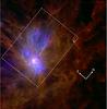 |
Fig. 1 Three-colour Herschel image of the Mon R2 molecular complex using 70 μm (blue), 160 μm (green), and 250 μm (red) maps. The shortest wavelength (blue) reveals the hot dust associated with H ii regions and protostars. The longest wavelength (red) shows the cold, dense cloud structures, displaying a filament network. The dashed rectangle locates the four H ii region area shown in Fig. 2. |
2. Data
2.1. Observations and data reduction
Mon R2 was observed by Herschel (Pilbratt et al. 2010) on September 4, 2010 (OBSIDs: 1342204052/3), as part of the HOBYS key programme (Motte et al. 2010). The parallel-scan mode was used with the slow scan-speed (20′′/s), allowing simultaneous observations with the PACS (70 and 160 μm; Poglitsch et al. 2010) and SPIRE (250, 350, 500 μm; Griffin et al. 2010) instruments at five bands. To diminish scanning artefacts, two nearly perpendicular coverages of 1.1° × 1.1° were obtained. The data were reduced with version 8.0.2280 of HIPE2 standard steps of the default pipeline up to level 1, including calibration and deglitching, and were applied to all data. The pipeline was applied (level-2) further, including destriping and map making, for SPIRE data. To produce level-2 PACS images, we used the Scanamorphos software package3 v13, which performs baseline and drift removal before regriding (Roussel 2013). The resulting maps are shown in Rayner et al. (in prep.). The map angular resolutions are 6″−36″, which correspond to 0.025−0.15 pc at the distance of Mon R2.
The Herschel 3-colour image of the Mon R2 molecular complex shows that the central UCH ii region, seen as a white spot in Fig. 1, dominates and irradiates its surroundings. Three other H ii regions exhibit similar but less pronounced irradiating effects (see the bluish spots in Fig. 1). These H ii regions develop into a clearly structured environment characterised by cloud filaments.
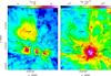 |
Fig. 2 Dust temperature (colours in a) and contours in b)) and column density (colours in b) and contours in a)) maps of the central part of the Mon R2 molecular cloud complex, covering the central, western, eastern, and northern H ii regions with 36″ resolution. The heating sources of H ii regions are indicated by a cross and with their name taken from Racine (1968) and Downes et al. (1975). Smoothed temperature and column density contours are 17.5, 18.5, and 21.5 K and 7 × 10²¹, 1.5 × 10²², 5 × 10²², and 1.8 × 1023 cm-2. |
2.2. Column density and dust temperature maps
The columm density and dust temperature maps of Mon R2 were drawn using pixel-by-pixel SED fitting to a modified blackbody function with a single dust temperature (Hill et al. 2009). We used a dust opacity law similar to that of Hildebrand (1983), assuming a dust spectral index of β = 2 and a gas-to-dust ratio of 100, so that dust opacity per unit mass column density is given by κν = 0.1 (ν/ 1000 GHz)β cm2 g-1, as already used in most HOBYS studies (e.g. Motte et al. 2010; Nguyen-Luong et al. 2013). The 70 μm emission very likely traces small grains in hot PDRs and so was excluded from the fits because it does not trace the cold dust used to measure the gas column density (Hill et al. 2012).
We constructed both the four-band (T4B) and three-band (T3B) temperature images and associated column density maps by either using the four reddest bands (160 to 500 μm) or only the 160, 250, and 350 μm bands of Herschel (cf. Hill et al. 2011, 2012). Prior to fitting, the data were convolved to the 36″ or 25″ resolution of the 500 μm (resp. 350 μm) band and the zero offsets, obtained from comparison with Planck and IRAS (Bernard et al. 2010), were applied to the individual bands. The quality of a SED fit was assessed using χ2 minimisation. Given the high quality of the Herschel data, a reliable fit can be done even when dropping the 500 μm data point. For most of the mapped points, which have medium column density and average dust temperature values, NH2 and Tdust values are only decreased by 10% and increased 5%, respectively, between T4B and T3B. In the following, we used the column density or temperature maps built from the four longest Herschel wavelengths, except when explicitly stated. The high-resolution T3B, I70 μm, and I160 μm maps have only been used for size measurements, not for profile-slope determinations.
Properties of the four H ii region bubbles of Mon R2.
The resulting column density map shows that the central UCH ii region has a structure that dominates the whole cloud with column densities up to NH2 ~ 2 × 1023 cm-2 (see Figs. 2b and F.1). In its immediate surroundings, i.e. ~1 pc east and west, as well as ~2.5 pc north, the temperature map of Fig. 2a shows two less dense H ii regions and one extended H ii region, respectively. The name and the spectral type of the stars that create these four H ii regions are taken from Racine (1968) and Downes et al. (1975). Three are associated with reflection nebulae and are called IRS1, BD-06 1418 (vdB69), BD-06 1415 (vdB67), and HD 42004 (vdB68) (see Figs. 2a, b, F.2 and Table 1). The central UCH ii region is located at the junction of three main filaments and a few fainter ones, giving the overall impression of a “connecting hub” (Fig. 2b). The three other H ii regions are developing within this filament web and within the UCH ii cloud envelope, which complicates study of their density structure.
The dust temperature image of Figs. 2a and F.2 shows that the mean temperature of the cloud is about 13.5 K and that it increases up to ~27 K within the three compact and ultra-compact H ii regions.Dust temperature maps only trace the colder, very large grains and are not sensitive to hotter dust present within H ii regions (see Anderson et al. 2012, Fig. 7). The temperature obtained from FIR Herschel SED corresponds to dust heated in the shell or PDR and thus directly relates to the size of the ionised bubble.
2.3. Radio fluxes and spectral type of exciting stars
We first estimated the spectral type of exciting stars from their radio fluxes. To do so, we looked for 21 cm radio continuum flux in the NVSS images (Condon et al. 1998), as well as in the corresponding catalogue4. The three compact H ii regions delineated by colours and the temperature contours of Fig. 2 all harbour one single compact 21 cm source (see Table 1). The more developed northern H ii region contains several 21 cm sources, whose cumulated flux can account for the total integrated emission of the region. We calculated the associated Lyman continuum photon emission, using the NVSS 21 cm flux listed in Table 1 and the formulae below, taken from Martín-Hernández et al. (2005), for example, 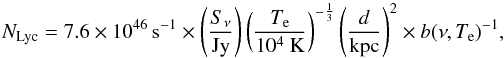 (1) where Sν is the integrated flux density at the radio frequency ν, Te is the electron temperature, d is the distance to the source, and the function b(ν,Te) is defined by
 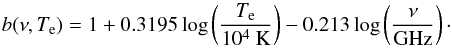 (2) Quireza et al. (2006) determined an electron temperature of ~8600 K for the central UCH ii region from radio recombination lines. We adopt the same temperature for the other H ii regions since this Te value is close to the mean value found for H ii regions (see e.g. Quireza et al. 2006, Table 1). Using the NLyc estimates of Table 1 and the calibration proposed by Panagia (1973), we assumed that a single source excites the H ii regions of Mon R2 and estimated their spectral type (see Table 1). These radio spectral types from B2.5 to B1 agree perfectly with those deduced from the visual spectra of Racine (19685; see Table 1). We calculated NLyc for the Mon R2 UCH ii region using six other radio fluxes with wavelengths from 1 to 75 cm available in Vizier. They all have radio spectral types ranging from O9.5 to B0, which also agrees with previous estimates (Massi et al. 1985; Downes et al. 1975). The concordance of spectral types derived from flux at different radio wavelengths, including the shortest ones, confirm the free-free origin of the centimetre fluxes with a limited synchrotron contamination.
2.4. H II region type classification
Wood & Churchwell (1989b, end of Sects. 4.a and 4.c.xi) previously classified Mon R2 as an UCH ii region. Considering the sizes and densities determined in Sect. 3.2, we define the morphological type of the four H ii regions. The values from the central H ii region (ρe = 3.2 × 103cm-3, RH ii = 0.09 pc) are compatible with the range of oberved values for UCH ii regions (e.g. Hindson et al. 2012), ρe = 0.34−1.03 × 104 cm-3 and RH ii = 0.04−0.11 pc. It agrees with the classification obtained from IRAS fluxes6. The western and eastern H ii regions have similar small sizes (around 0.1 pc) but lower densities (<1000 cm-3), which we assume to be more characteristic of compact H ii regions. The northern H ii region is larger (close to 1 pc) and has the very low density (<100 cm-3) typical of extended H ii regions.
3. Modelling of the H II regions’ environment
The initial dense cloud structures inside which the high-mass protostars have been formed and the H ii regions that have developed could have been considerably modified by both the protostellar collapse and the H ii region ionisation. The bubble and shell created by the expansion of H ii region retains information about its age and the mean density of the inner protostellar envelope whose gas has been ionised or collected. We hereafter investigate all of the components needed to describe the environment of H ii regions. The density model is presented in Sect. 3.1. We first focus on the inner components that are directly associated with H ii regions and which are generally studied at cm-wave radio, optical, or near-infrared wavelengths (see Sects. 3.2 and 3.3). We then characterise the component best studied by our Herschel data in detail, namely the surrounding cold neutral envelope (Sect. 3.4). We finally jointly use all available pieces of information to perform a complete density modelling in Sect. 3.5.
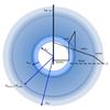 |
Fig. 3 H ii region and its surrounding four-component spherical model and radial profile of density (right). The ionised bubble is first surrounded by the shell containing all of the swept-up material. The neutral envelope is made of two parts with different density gradients finally merging into the background. The short dashed line represents the extrapolation of the inner envelope before the ionisation expansion and collecting process. |
3.1. Model of H II regions and their surroundings
Modelling of the observed column density and temperature structure of H ii regions and their surroundings (Fig. 2) requires four density components (see Fig. 3): a central ionised bubble, a shell concentrating almost all of the collected molecular gas, a protostellar envelope decreasing in density, and a background. The background corresponds to the molecular cloud inside which the H ii region is embedded. The three other components are proper characteristics of the H ii region and its envelope. The envelopes of the three compact and UCH ii regions are not correctly described by a single power law, but require two broken power laws similar to that of the inside-out collapse protostellar model (Shu 1977; Dalba & Stahler 2012; Gong & Ostriker 2013).
3.2. Extent of H II regions
H ii region sizes are important for measuring because they constrain the age and evolution of the regions. Sizes are generally computed from Hα or radio continuum observations that directly trace the ionised gas. Such data are not always available. Potentially, Hα could be attenuated for the youngest H ii regions, and radio continuum surveys frequently have relatively low resolution. We can instead use Herschel temperature maps, as well as 70 μm and 160 μm images to estimate the size of the H ii regions.
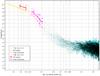 |
Fig. 4 Dust temperature radial profiles of the central UCH ii region showing a steep outer part and a flatter inner region. We note the agreement of the measurements done with the 3-band temperature map, T3B (red and magenta lines and points), and with the 4-band temperature map, T4B (yellow and pink lines and points). |
The extent of all four H ii regions can clearly be seen in the dust temperature map shown in Fig. 2a. This is an indirect measure since the Herschel map traces the temperature of big dust grains that dominate in dense gas and which reprocess the heating of photo-dissociation regions (PDRs) associated with H ii regions. Such a dust temperature map provides the temperature averaged over the hot bubbles in the H ii region and colder material seen along the same line of sight. This is particularly clear when inspecting the western H ii region, which is powered by BD-06 1415, since its temperature structure is diluted and distorted by the filament crossing its southern part. We used both the T4B and T3B temperature images with 36″ and 25″ resolutions. For the large northern extended H ii region, the T4B map alone would be sufficient since the angular resolution is not a problem. For the three other H ii regions, we need to use the T3B map, as well as 70 μm and 160 μm maps where intensities are used as temperature proxies (see discussion by Compiègne et al. 2011; Galliano et al. 2011). The 70 μm emission traces the hot dust and small grains in hot PDRs, which mark the borders of H ii regions and thus define their spatial extent.
Despite the inhomogeneous and filamentary cloud environment of the Mon R2 H ii regions, the heated bubbles have a relatively circular morphology (see Fig. 2a).This is probably due to the ionisation expansion, which easily blows away filaments and dense structures (e.g. Minier et al. 2013). To more precisely define the H ii region sizes, we computed temperature radial profiles azimuthally averaged around the heating and ionising stars, which are shown in Figs. 2a, b. The resulting temperature profiles of the four H ii regions share the same general shape: a slowly-decreasing central part surrounded by an envelope where the temperature follows a more steeply decreasing power law (see e.g. Fig. 4). We used the intersection of these two temperature structures to measure the radius of the flat inner part, which we use as an estimator of the H ii region radius, RH ii (see Table 1). At the junction between the two temperature components, data scattering and deviation from a flat inner part leads to uncertainties of about 15%. The higher resolution T3B, 70 μm, and 160 μm maps confirm the derived RH ii values and reach a confidence level of ~10% uncertainty.
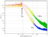 |
Fig. 5 Radial intensity profiles of the central UCH ii region showing the measurements done at 70 μm (blue points) and 160 μm (green points) taking advantage of the PACS highest resolution, compared with the 3-band temperature (T3B) and the 4-band temperature (T4B) data given by the black arrow. The 160 μm profile decreases less in the inner part of the envelope (pink line) than in its outer part (yellow line). Since 160 μm emission is sensitive to dust temperature and density, this behaviour is probably related to the two different slopes found for the density profile of the envelope characterised in Sect. 3.4.1. The slope change indeed occurs at similar RInfall radius. |
For the (small) central UCH ii region, the radial profiles of the T3B and T4B temperatures are shown in Fig. 4. The flux profiles obtained from the 70 μm and 160 μm imageswith 6″ and 12″ resolutions are shown in Fig. 5. These four different estimators display similar radial shapes for the H ii region and give consistent size values: RH ii ≃ 0.09, 0.08, 0.09, and 0.09 pc for 70 μm, 160 μm, T3B, and T4B, respectively. Similarly, concordant measurements are found for the fully resolved northern H ii region in the T4B and T3B maps: RH ii ≃ (0.85 ± 0.05) pc. Interestingly, for the central UCH ii region, the derived RH ii value of ~0.09 pc is in excellent agreement with the one deduced from H42α RRL measurements (~0.08 pc, see Pilleri et al. 2012), showing that hot dust and ionised gas are spatially related.Radio continuum data and infrared [Ne ii] line also give similar sizes and shapes (Massi et al. 1985; Jaffe et al. 2003).
Using Lyman flux (Table 1 Col. 7) and H ii region size (Table 1 Col. 9) we use Eq. (5) to compute the corresponding electron density ρe, given in Col. 10.
3.3. H II region shells and their contribution to column density
Dense shells have been observed around evolved H ii regions within simple and low-column density background environments (e.g. Deharveng et al. 2005; Churchwell et al. 2007; Anderson et al. 2012). The “collect-and-collapse” scenario proposes that the material ionised by UV flux of OB-type stars is indeed efficiently sweeping up some neutral gas originally located within the present H ii region extent and developing a shell at the periphery of H ii bubbles (Elmegreen & Lada 1977).
In Appendices D and E we investigate the contribution of this very narrow component to the column density measured with Herschel. Appendix D shows the beam dilution of the column density expected from the shell shoulder. Appendix E explores the density attenuation due to bubble and shell expansion in different types of envelope density profile. These two effects combined reduce the importance of the shell and predicts a decrease in the observed column density of H ii regions with expansion at least in decreasing-density envelopes. The shell of the central UCH ii region characterised by Pilleri et al. (2014, 2013) has an unnoticeable contribution to the high column density of the envelope. Even in the northern region, which is the most extended and favourable to the detection of a shell, the shell characteristics are uncertain due to the filamentary environment inside which the H ii region developed (see Fig. 8). It shows that the shell is not a dominant component of the column density structure of the H ii regions studied here, but it cannot be neglected a priori from modelling.
3.4. The envelope surrounding H II regions
Amongst the crucial parameters influencing the expansion of an H ii region and the size of the heated/ionised regions, we need to characterise the density profiles of their neutral envelopes. We therefore constructed radial column density profiles by plotting the NH2 map around each of the ionising sources shown in Fig. 2b. Figures 6 shows the column density profiles of the central UCH ii and eastern H ii regions, respectively. The colours used for the different radial parts of the profiles are similar to those used for the temperature profiles of Fig. 4.
Radial column density profiles exhibit relatively flat inner parts that provide a reliable measurement of the column density maximum value,  , of the envelope surrounding each of the four H ii regions (see Table 3, Col. 7). The sizes of these envelopes, given by the radius at half maximum, RHM, were measured on the column density profile and range from 0.35 pc to 1.5 pc (see Table 3, Col. 8).
Assuming a spherical geometry that agrees with the shape of H ii regions studied here, for which RHM can be used as a size estimator, we can roughly estimate the observed mean density, ⟨ ρobs ⟩, from the maximum of the surface density , using the equation 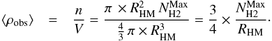 (3) This mean density corresponds to the presently observed state of the envelope (see Table 3, Col. 9). To estimate the initial mean density of the envelope, ρinitial, before the ionisation starts, Sect. 3.5 suggests another way to determine it through its actual maximum density and density profile slope.
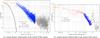 |
Fig. 6 H ii region bubble (yellow line and points) surrounded by a neutral gas envelope splitting into slowly and sharply decreasing NH2 parts (pink and blue lines and points). The background is defined by the lower limit of the clouds of grey points. The resolution corresponding to the Herschel beam at 500 μm is illustrated by the black curve in a). |
Comparison of the central UCH ii region’s characteristics shows good agreement, as deduced here with the parameters of the model used by Pilleri et al. (2012). The model has an envelope size of 0.34 pc, inner radius of 0.08 pc, and a mean density ~ 0.8 × 105 cm-3 comparable to our estimates: RH ii ~ 0.09 pc RHM ~ 0.35 pc, ⟨ ρobs ⟩ = 1.4 × 105 cm-3.
3.4.1. Column density profiles
With the model of Fig. 3 in mind, we characterise the four main components associated with H ii regions and their surroundings in detail. The H ii region bubble, fitted by a yellow line, corresponds to a temperature plateau and has an almost constant column density in Fig. 6. Surrounding the H ii region, one can find the cloud envelope, which has a constantly decreasing temperature profile and splits here into slowly and sharply decreasing NH2 parts, fitted by pink and blue lines in Fig. 6. As for the eastern H ii region, the column density is lower and the inner envelope extent is larger, allowing a better distinction between the different envelope parts than in the central UCH ii region. In this context, we define the inner envelope as the part where the column density slowly decreases and the external envelope as the one with a steeper decrease. The crossing point between these two envelope components defines the outer radius of the inner envelope, called RInfall for reason explained in Sect. 5.2. Its values are given in Table 3.
The profile analysis is trustworthy for the central UCH ii region since it is prominent and azimuthally averaged over 2 π radians. The analysis is cruder for the three other H ii regions developing between filaments (see Fig. 2b). For these H ii regions, we have selected inter-filament areas and quadrants that represent the H ii regions best and avoid the ambient filamentary structure (see Fig. F.1). By doing so, we aimed to measure the contribution of the H ii region envelope alone. We have checked, mainly in the case of the eastern region, that varying the azimuthal sectors selected between the major filaments does not change either the radii or the slope of the envelopes by more than 20%. However, contamination by other overlying cloud structures cannot be completely ruled out, and some studies of other isolated prominent H ii regions are needed to confirm the results presented here.
The column density slopes of both the internal and the external envelopes can be represented well by power laws such as N(θ) ∝ θp (see Fig. 6). Since the column density is the integration of the density on the line of sight, we can logically retrieve their density profiles through measuring the column density profiles. For a single power law density ρ(r) ∝ rq, an asymptotic approximation leads to a very simple relation between the q index and the power law index of the column density profile described as N(θ) ∝ θp: q ≃ p−1. This assumption holds for piecewise power laws that match a large portion of the observed envelopes. It is the case of external envelopes as is confirmed in Sect. 3.5. However, for small pieces like the inner envelopes, the conversion from column density to density power law indices is more complex (see Yun & Clemens 1991; Bacmann et al. 2000; Nielbock et al. 2012).
Towards the centre, at an impact parameter7 smaller than the H ii region outer radius, all four density components contribute to the observed column density. Then a gradual increase in the impact parameter progressively reduces the number of the contributing density components. The four structural components of Fig. 3 were constrained, step by step, from the outside/background to the inside/H ii region bubble.
We first estimated the background column density arising from the ambient cloud using both near-infrared extinction (Schneider et al. 2011) and the Herschel column density map (Fig. F.1). They consistently give background levels of Av ~ 0.5 mag8 at the edge of the Herschel map. To minimise the systematic errors in determining the slope of the outer envelope, a 0.5 mag background was subtracted from the column density profiles. For the northern H ii region, the power law slope measured for the envelope remains well-define with p possibly ranging from −0.4 to −0.5, although the background contribution to the observed column density profile is the most important.
We simultaneously estimated the power law coefficients of the two parts of the envelope from the slopes (p) measured on “background-corrected” column density profiles. We used the relation q ≃ p−1 to measure the density profile slopes (q) of the outer envelope and obtain a first guess for the inner envelope. Tables 3 and 2 list some of the parameters derived from our column density structural analysis.
Comparison of the properties of the neutral envelopes surrounding the four H ii regions of Mon R2.
The outer envelope of the two compact eastern and western H ii regions displays a column density index of pout ≃ −1 with an uncertainty of 0.2 (~3σ), which corresponds to a ρ(r) ∝ r-2 density law. The central UCH ii region itself exhibits a steeper density gradient in its outer envelope with qout ≃ −2.5. In practice, the uncertainties are such that the slopes are well defined within an uncertaintiy of about 10% or ~0.2, clearly allowing the distinction between ρ(r) ∝ r-2 and ρ(r) ∝ r-1.5 or ρ(r) ∝ r-2.5 power laws. This is a clear improvement from the studies made before Herschel from single band sub-millimetre observations (e.g. Motte & André 2001; Beuther et al. 2002; Mueller et al. 2002).
The northern H ii region, whose envelope does not split into an inner and outer parts, has a decreasing density profile up to 0.8 pc with a power law coefficient of q ≃ −1.5.
The internal envelopes of the central, eastern, and western H ii regions have a column density profile with power law coefficients pin ≃ −0.35 ± 0.2, but the conversion is not straigthforward and the density modelling made in Sect. 3.5 is needed to derived correct values.
3.5. Density modelling
We here perform a complete modelling of the observed column density profiles to adjust and evaluate the relative strength and the characteristics of the components used to describe H ii regions and their surroundings. We modelled four different components along the line of sight to reconstruct the observed column density profile. We used the size and density profiles derived in previous sections and listed in Table 3 to numerically integrate between proper limits, along different lines of sight, the radial density profiles of the background, envelope (external then internal), H ii region shell, and bubble. For a direct comparison with observed profiles, we convolved the modeled column density profiles with the 36′′ resolution of the HerschelNH2 maps. Figures 7, 8 display the calculated column density profiles of each of the four aforementioned structural components and the resulting cumulative profile. Figure F.1 also locates, with concentric circles, the different components used to constrain the structure of the central UCH ii region.
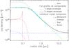 |
Fig. 7 Column density profile of the central UCH ii region (cyan diamonds with σ errors bars) compared to models with all components illustrated in Fig. 3. The neutral envelope with two density gradients or with a single one are shown by a black line and a dotted black line respectively. An envelope model with a single density gradient cannot match the observed data. Individual components after convolution by the beam are shown by magenta, red, green, and blue dashed lines, for the bubble, shell, envelope and background. The continuous red line shows the unconvolved shell profile at an infinite resolution. |
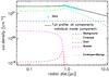 |
Fig. 8 Column density profile for northern H ii region and its four components coded with the same colours as in Fig. 7. The dotted green line corresponding to the sum of the envelope and background contributions matches well with observed data. |
Properties of the neutral envelopes surrounding the four H ii regions of Mon R2.
We recall that the background is itself defined as a constant-density plateau: AV ~ 0.5 mag for all H ii regions. The background, even if faint, has an important relative contribution towards the outer part of the H ii region structure, where the envelope reaches low values. For the northern H ii region, the background contribution to the observed column density profile is almost equal to that of the envelope, as it can be seen on the reconstructed profile of Fig. 8.
Our goal is to estimate for each of the four H ii regions in Mon R2, the absolute densities of the envelope, shell, and H ii region bubble (see Tables 1−3).
We adjusted our model to the complete column density profile, progressively adding the necessary components: outer envelope, inner envelope, shell and bubble, the latter first assumed to be empty. In Table 2 we compare the results directly obtained from observationnal data and from data modelling.
We first modeled the density profile observed at radii greater than 1 pc, dominated by the outer envelope density. We jointly adjusted the density at 1 pc, ρ1 and the density power law slope, qout. The qout values derived from the q = p−1 relation are in excellent agreement with the fitted ones. The ρ1 values obtained are very similar to those calculated with Eqs. (B.3) and (B.4) from the column density values at 1 pc and the appropriate qout values. Our results prove that the asymptotic assumption is correct for the outer envelope component. The characteristics of the inner envelope, which are mixed on the line of sight with those of the outer envelope, is only reachable through modelling. Figures 7, 8 show that once the envelope density structure is fixed, the modelled column density profile fits the observed one for radii larger than RH ii nicely.
The shell and the bubble are expected to have a weak influence on the profiles of the ultra-compact-to-compact H ii regions (here the central, eastern, and western regions). Indeed, the H ii bubble sizes and the amount of gas mass collected in the shell are so small that their contribution can be almost neglected, and high resolution would be needed to observe the narrow shoulder enhancement at the border of the shell (see Fig. D.1). These two components are, however, definitely needed to reproduce the central column density of the more extended and diffuse, northern Extended H ii region. Figure 8 displays an inner column density plateau and a tentative shoulder of the column density profile just at the RH ii location. We have estimated an upper limit to the mean density, column density, and mass for the northern H ii region swept-up shell, assuming a 0.01 pc thickness with a density varying from 50 to 1000 cm-3:  cm-2, and 3 M⊙. This putative shell is, however, difficult to disentangle from the envelope border and the complex cloud structure in this area.
According to Hosokawa & Inutsuka (2005), the central bubble should be devoid of cold dust in the earliest phase of H ii region development, roughly corresponding to the compact H ii phase. In the case of the central UCH ii region, we used the electron density of 1.6 × 103 cm-3 (Quireza et al. 2006) as an upper limit for the H ii bubble density of neutral gas. Even this relatively high density value results in a negligible contribution to the modelled column density profile (see Fig. 7). For the northern H ii region, a low-density (~50 cm-3) central component needs to be introduced in the bubble to reconcile the modeled profile and the observational data. Without it, we would observe a relative hole or depletion in the centre of the column density profile (see red and green lines in Fig. 8 compared to cyan or black ones). The uncertainties are such that the exact value of the inner density component of the northern H ii region is not known better than to a factor of ten. Therefore, our modelling can only give upper-limit densities for the bubble gas content and H ii region shell.
Table 3 lists the adopted values of the envelopes density characteristics. The envelope density at 1 pc radius, i.e. ρenv(r = 1 pc), which was used to scale the parametrised density profile, defines the absolute level of density in the envelope. It also gives the density observed at the inner border of the envelope, i.e. ρenv(r = RH ii), corresponding to the maximum value measured now in the envelope. The central density of the eastern Compact H ii region is a bit weak and atypical. For the northern H ii region, the inner border of the envelope is at RH ii ~ 0.8 pc, and we can extrapolate the ρ(r) ∝ r-1.5 density profile to a distance of 0.1 pc: ρestimated(r = 0.1 pc) ~ 6.6 × 103 cm-3. We also considered the density at much smaller radii, which would correspond to the inner radius of the extrapolated protostellar envelope and the central core density: ρenv(r = 0.005 pc/1000 AU), Col. 4 in Table 4.
All inner envelopes have a power law slope that is smaller than or equal to the expected infall value of 1.5. The values lower than 1.5 could be due to sub-fragmentation in the inner envelope. Some indications of inhomogeneous clumpy structures are indeed revealed by high-resolution maps (Rayner et al., in prep.). All outer envelopes have power law slopes greater than or equal to the expected SIS value of 2, corresponding to hydrodynamical equilibrium. The high value observed for the central H ii region could be due to additional compresion (Sect. 5.1, Appendix C). All these density determination will be used below to estimate the mean initial neutral gas density before the ignition of an H ii region.
4. Ionisation expansion time
The physical characteristics presented in the previous sections are used here to constrain the expansion time of the ionisation bubble in its neutral envelope. In Sect. 4.1, analytical calculations without gravity show that the average initial density, ⟨ ρinitial ⟩, is the main parameter dictating the expansion behaviour. In Sect. 4.2, simulations are compared to analytical results of Sect. 4.1 to determine the impact of gravity on expansion. In constant high-density envelopes, gravity prevents expansion through quenching or re-collapse, but in a decreasing-density envelope, the impact of gravity becomes negligible once the expansion has started. We thus conclude in Sect. 4.3 that analytical calculations without gravity can be used to derive valid ionisation expansion times.
4.1. Strömgren-sphere expansion analytical calculations
Differences in size between the northern and the western H ii regions, which harbour an exciting star of the same spectral type, tend to suggest that the northern H ii region is more evolved than the western one (see Fig. 2a and Table 1). The larger number of striations observed in the visible image of the northern reflection nebula also indicate an older stage of evolution (Thronson et al. 1980; Loren 1977).
To confirm these qualitative statements, we here determine time differences in the beginning of the ionisation expansion H ii regions for the four H ii regions. We recall that the deeply embedded central UCH ii region has no optical counterpart, while the western, eastern, and northern H ii regions are respectively associated with the vdB67, vdB69, and vdB68 nebulae.
Estimations of expansion time for the four H ii regions of Mon R2.
4.1.1. Average initial density
The density observed at the inner border of the envelope (i.e. ρenv(r = RH ii), corresponding to the maximum value measured now in the envelope) can be used to estimate the density the protostellar envelope had at the time of the ignition of the ionisation, when averaged within a sphere of RH ii radius. Given the inner density structure observed for the four H ii regions envelopes, whose density gradient is described by ρ(r) ∝ rqin, the mean density of the initial envelope part, which is now mostly collected in the shell, is given by 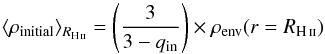 (4) and derived in Appendix A.1. It is the most important parameter for analytical calculations, and its calculated values are given in Col. 2 of Table 4.
4.1.2. Expansion in an homogenous density static envelope
Spitzer (1978) predicted the expansion law of a Strömgren sphere and thus the evolution of the H ii region size with time in an homegeneous medium (see also Dyson & Williams 1980 and Arthur et al. 2011, Eq. (1)). Following Ji et al. (2012), we inverted the relation and expressed time since the ignition of the ionisation as a function of the observed H ii region radius, RH ii: ![\begin{equation} \label{exptime} t_\text{Spitzer}(R_{\rm \ion{H}{ii}}, \langle\rho_\text{initial}\rangle)= \frac{4}{7} \times \frac{R_{\rm Str}}{c_{\rm s}} \left[\left( \frac{R_{\rm \ion{H}{ii}}}{R_{\rm Str}} \right)^{7/4} - 1 \right] , \end{equation}](/articles/aa/full_html/2015/12/aa26239-15/aa26239-15-eq210.png) (5) where cs = 10 km s-1 is the typical sound speed in ionised gas, and RStr is the radius of the initial Strömgren sphere (Strömgren 1939, 1948). The latter is given by the following equation
(5) where cs = 10 km s-1 is the typical sound speed in ionised gas, and RStr is the radius of the initial Strömgren sphere (Strömgren 1939, 1948). The latter is given by the following equation 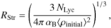 (6) or in numerical terms
 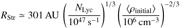 (7) where ⟨ ρinitial ⟩ is the initial mean density in which the ionisation occurs, NLyc is the number of hydrogen ionising photons from Lyman continuum and αB = 2.6 × 10⁻¹³ cm3s-1 is the hydrogen recombination coefficient to all levels above the ground.
The ionisation ages determined from Eq. (5) strongly depend on the mean initial density, ⟨ ρinitial ⟩ (see its definition in Sect. 4.1.1), since it defines the initial radius of the ionised sphere, RStr (see Eq. (6)). With the assumption that the expansion develops in a constant-density medium, the ionisation age is strictly determined by the initial and present sizes of the ionised region, RStr and RH ii (see Eq. (5)).
Initial density estimates are very uncertain since they depend on assumptions made for the gas distribution before protostellar collapse and its evolution conditions. Nevertheless, the envelope density structure can be approximated by the mean density of the envelope part, which was travelled through by the ionisation front expansion and has been collected in the shell.
Considering the maximum density of the different H ii region envelopes at their inner border (RH ii) and using Eq. (4), we calculate an initial mean density (⟨ ρinitial ⟩ H ii) reported in Col. 2 of Table 4. Assumed to be representative of an envelope with an equivalent homogenous constant density, this value is jointly used with the ionising flux given in Table 1 to calculate the corresponding expansion time with Eq. (5) and is given in Col. 3 of Table 4. The expansion time of compact and UCH ii regions are similar (tExp ~ 20−90 × 103 yr) with a range that is mainly due to different initial densities. The northern extended H ii region is three to 15 times older (~300 × 103 yr), in line with what is expected from their size differences.
4.1.3. Expansion in a density decreasing static envelope
The present study shows that H ii regions develop into protostellar envelopes whose density decreases with radius (see Sect. 3.5, see also introduction in Immer et al. 2014). The equation given by Spitzer (1978) describing their expansion in a medium of homogeneous density (Eq. (5)) therefore does not directly apply. We calculated the expansion of an ionised bubble in an envelope with a density profile following a power law. We included in this envelope a central core with a rc radius and a constant density of ρc. The clump density structure thus follows  (8) where ρ1 is the density at 1 pc deduced from the constructed density profile or directly measured from the column density at the same radius (see Sect. 3.5). The expansion as a function of time in a decreasing envelope is derived by calculations detailed in Appendix A.2. In close agreement with previous work by Franco et al. (1990), it is given by
 ![\begin{eqnarray} \ \label{exptimeDecrEnv} t_q(R_{\rm \ion{H}{ii}}) & = &\frac{4}{7 - 2q} \times \frac{r_\text{c}^{7/4}} {{R_{\rm Str}}^{3/4}} \frac{1}{c_{\rm s}} \left[\left( \frac{R_{\rm \ion{H}{ii}}}{r_{\rm c}} \right)^{{7{-}2q}/4} - 1 \right]\\ & = & \frac{4}{7 - 2q} \times \frac{r_\text{c}} {V(r_{\rm c})} \left[\left( \frac{R_{\rm \ion{H}{ii}}}{r_{\rm c}} \right)^{{7{-}2q}/4} - 1 \right] \nonumber \end{eqnarray}](/articles/aa/full_html/2015/12/aa26239-15/aa26239-15-eq222.png) (9) with the same definitions as in Eqs. (5), (6) and where
(9) with the same definitions as in Eqs. (5), (6) and where 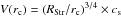 is the shell expansion speed at the homogeneous core radius rc. For a constant density, which is the Spitzer case, q = 0 and rc = RStr, and Eq. (9) resumes to Eq. (5).
The inner envelope density profiles of the four regions have gradients which at most corresponds to the free-fall case, with a power law coefficient of q ≲ 1.5. For higher values (q> 1.5), Franco et al. (1990) showed that expansion is in the so-called “champagne” phase. In such cases, there is neither velocity damping nor creation of a collected shell (see also Shu et al. 2002; Whalen & Norman 2006). In contrast, the shell and low expansion velocity observed for the central UCH ii region (Fuente et al. 2010; Pilleri et al. 2012, 2013, 2014) indicate that q = 1.5 is probably an upper limit. The ionisation front should then stay behind the infall wave, RH ii<RInfall, with the expansion starting at supersonic velocities, classically ~10 kms-1, but then quickly damped to values around the sound speed in the neutral molecular medium. As a matter of fact, the expansion of the central UCH ii slowed down to ~1 kms-1 at ~0.08/0.09 pc (Pilleri et al. 2014, and references therein), so far behind the infall wave situated around 0.3 pc(see Table 3). More generally, in the case of the four H ii regions of Mon R2, even if the initial ionisation extension exceeded the central core size RStr>rc, ionisation would expand in internal infalling envelopes with shallow (q< 1.5) density profiles. The ρ1 value used in Eq. (8) corresponds to the internal envelope, ρint(1pc), and is calculated from the one observed in the external envelope, ρenv(1pc), by the relation 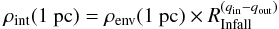 (10) where ρenv(1 pc), RInfall, qin, and qout are given in Table 3.
For the central core, we adopted a size of 0.005 pc (~1000 au), which is meant to represent the size where the spherical symmetry is broken. Since 3D effects are beyond the scope of this paper, gas on small scales (<0.005 pc) is represented by an homogeneous and constant density medium. This value is between the typical size of Keplerian disks surrounding low-mass pre-main sequence T Tauri stars (~0.001 pc, 200 au, Carmona et al. 2014; Maret et al. 2014; Harsono et al. 2014) and the largest disks or flattened envelopes observed around intermediate- to high-mass Herbig Ae-Be stars (0.01 pc, 200−2000 au, Chini et al. 2006; de Gregorio-Monsalvo et al. 2013; Jeffers et al. 2014). Calculations with various rc values in the conditions considered here (q ≲ 1.5) show that when rc ≪ RH ii, the value of rc does not have much influence on the expansion time of the ionised bubble.
For objects studied here, the initial size of the Strömgren sphere, RStr, is always smaller than the core radius, rc. Therefore the expansion is decomposed in two phases: the expansion in an homogenous medium of constant density, ρc from RStr up to rc and the expansion in the decreasing density part of the envelope between rc and RH ii. The expansion time of the first phase in the central core, tc, is given by the Spitzer formula (Eq. (5)), and the second phase in the decreasing density envelope, td, is given by Eq. (9). The total expansion time texp = tc + td, is given in Col. 5 of Table 3. It is consistent with the value obtained for an expansion within a homogenous-density medium with an equivalent mass (see Col. 3), corroborating the constant-density equivalence hypothesis and the calculation performed in Sect. 4.1.2. Agreement is better for the compact or UCH ii regions, which have ⟨ ρinitial ⟩ closer to ρc than the extended northern region.
The time for an H ii region to expand depends strongly on the density gradient in the inner envelope through the density extrapolated for the 0.005 pc core, ρc, which determines the Strömgren radius, RStr. The gradient index, qin, itself gives the transit time in the envelope, td. All measures are uncertain, especially because the H ii region expansion occurred in an envelope whose density may be higher than the one presently observed. If ionisation expansion took place in a primordial envelope with a density slope typical of free-fall, qin = 1.5, then the calculations would give a minimum age of 105 yr for all three compact and UCH ii regions.
4.2. Simulations of H II regions development with gravity
We used dedicated simulations to assess the impact of a decreasing density and the effect of gravity on our estimates of the ionisation expansion time. We employed the HERACLES9 code (e.g. González et al. 2007), which is a three-dimensional (3D) numerical code solving the equations of hydrodynamics and which has been coupled to ionisation as described in Tremblin et al. (2012a,b). The mesh is one dimensional in spherical coordinates with a radius between 0 and 2 pc and a resolution of 2 × 10⁻³ pc, corresponding to 10 000 cells. The boundary conditions are reflexive at the inner radius and allow free flow at the outer radius. The adiabatic index γ defined as P ∝ ργ is set to 1.01, allowing us to treat the hot ionised gas and the cold neutral gas as two different isothermal phases.
The effects considered here are 1) the ionisation expansion and 2) the gravity of the central object. The envelope is considered at rest at the beginning of the simulation, but when gravity is taken into account the infalling part of the envelope has a velocity close to the expected values.
Our models consider the gravitational effects of the ionising star but not that of the whole cloud, which could collapse under its own gravity. Such gas infall is important but modelling it is beyond the scope of this paper. It requires complex 3D turbulent simulations with self-gravity such as those developed in Geen et al. (in prep.). Their main conclusion is that global cloud infall can stall the expansion of H ii regions but do so less efficiently than 1D arguments. Indeed, infall gas should generally be inhomogeneous and clumpy, and the H ii region should expand in directions where fewer dense clumps are present.
Realistic winds from early B type stars have been checked to make certain they do not quantitatively modify the ionisation expansion time. A wind cavity in the ionised gaz would indeed only marginally increase the electronic density.
Important leaking and outflows of ionised matter would have a noticeable impact and is observed neither in the temperature map as seen by Anderson et al. (2015) for RCW120 nor in the hydrogen RRL or the radio data. Disruption of the molecular cloud thus cannot be important in the UCH ii region. Moreover, the ionising photon flux we used comes from the H ii region cavity. Any leaking of ionised matter would decrease the amount of ionised gaz in the cavity and thus increase the expansion time.
Complex structure and motions of the ionised gas have been reported by Jaffe et al. (2003) and modelled by Zhu et al. (2005, 2008). They argue for tangential motions of the ionised gas along the surface of the H ii region, which cannot suppress the thermal pressure at the origin of the expansion evolution. Thermal turbulence of ionised gas, the prime driver of expansion, is taken into account in simulations. Recent works show that introducing additional turbulence does not affect the H ii region expansion much because it would only increase the expansion time weakly (see Arthur et al. 2011; Tremblin et al. 2012a, 2014b).
Taking all these complexities and secondary effects into account is beyond the scope of the present paper since we merely tried to reproduce an overall behaviour, using the mean density at the origin. Detailed studies would require to take departure from spherical symmetry on small scales into account.
Simulations are based on 1) the density profiles derived from column density and 2) UV ionizing fluxes deduced from radio data. Temperature or electronic density are not used in the initial conditions so any changes of their values would not affect the simulation results.
For comparison, we used the profiles presented in Sect. 4.1.3 to perform simulations of H ii regions expanding within decreasing density envelopes without taking the gravity into account. The results given in Col. 6 of Table 4 agree within 15% with analytical calculations given in Col. 5. The remaining differences arise from assumptions made in the analytical solutions, which neglect the inertia of the shell and strong external pressure. These expansions are illustrated in Figs. 10, 11 by black lines.
We hereafter investigate the effect of gravity. Section 4.2.1 shows that extrapolating density profiles as done for analytical calculations of Sect. 4.1.3 would lead to quenching or recollapse for the central, western, and northern H ii regions. For the eastern region, the extrapolated low central density is not high enough for gravity to impede expansion, so expansion time remains similar. In Sect. 4.2.2, we calculate the maximum constant-density medium inside which the H ii regions could develop. Unrealistic envelope models with constant density would induce re-collapse even on a large scale, but they nevertheless provide useful upper limits to the ionisation expansion time. The case of the less dense northern and eastern H ii regions is discussed again in Sect. 4.2.3, and we confirm that once the expansion starts, the gravity influence is negligible, at least in decreasing-density envelopes. In Sect. 4.2.4, we summarise the results we obtained from simulations and give estimates of the ionisation expansion time for the four H ii regions in Mon R2.
4.2.1. Effect of gravity: quenching or recollapse
Introducing gravity due to the central object in the simulations results in the quenching (also called “choke off” by Walmsley 1995) of three H ii regions discussed here, and they expand in high-density media: central, western, and northern regions. They cannot develop and are quenched or gravitationally trapped (Keto 2007), even with the introduction of a realistic wind support arising from early B-type stars.
The eastern H ii region is not quenched and can develop in the observed inner envelope, which has a weak density gradient. The values of ⟨ ρinitial ⟩ and even ρc are lower than the maximum constant density ⟨ ρinitial ⟩ Max (see Table 4), explaining why quenching is not occurring here. In this case of a low-density envelope, the expansion time obtained in simulation without gravity (23 kyr, see Col. 6 of Table 4) is identical when including gravity in simulation (24 kyr, see Col. 9 of Table 4).
To allow expansion of the three H ii regions quenched in simulations, one needs to decrease the central density of the profile, ρc. If we keep extrapolating the density profile observed for the outer envelope (see ρ1 in Col. 10 of Table 3), the only way is to increase the constant density core radius, rc. This determines the maximum central density value,  , and the corresponding minimum core radius,
  , allowing an H ii region to develop up to the observed size. For the UC (central) and the compact (western) H ii regions, is larger than RH ii, corresponding to an expansion in a homogenous medium of density . The highest density observed in the envelope at a radius corresponding to the H ii region size is thus greater than the maximum density allowed by this scenario,
  , and the radii of constant density are larger than the actual H ii region sizes, rc>RH ii. Even if these assumptions are unrealistic, they are useful to determine upper limits. Another way to reduce the central density, as shown in Eq. (8), is to keep the same central core radius but decrease the density of the entire profile through the ρ1 value. This configuration implicitly assumes a mean envelope density at the initiation of the H ii region expansion that is lower than expected.
Figure 10 shows four simulations for the central UCH ii region. The expansion in a decreasing-density envelope with no gravity (black lines) is compared to two simulations including gravity and occurring in constant-density envelopes. For a constant low-density envelope (cyan curve) expansion can reach the observed H ii region size. For higher constant density (red dashed curve), the re-collapse occurs earlier and closer, preventing the expansion up to its present size. Increasing the density gradient of the inner envelope from that presently observed (qin = 0.85, continuous black line) to that expected for free-falling gas (qin = 1.5, dotted black line) increases the extrapolated density and thus the expansion time.
Figure 11 gives the expansion behaviour of five simulations for the northern H ii region. As in Fig. 10 and with the same colours, three simulations describe expansion within a decreasing density envelope without gravity (black line) and expansion in constant high- and low-density envelopes without gravity (dashed red and continuous cyan curves, respectively). Two additional simulations in a decreasing density envelope with gravity are displayed by a blue line for the nominal average initial density and a dashed blue line for a lower density.
Figure 9 shows the velocity field of a simulation for the northern region obtained at three different times. The simulation includes the gravity of the central ionising object in a density decreasing envelope with a central core of 0.05 pc and a density of 110 cm-3 at 1 pc. This envelope has a mean density in agreement with the observed characteristics (see Table 3). It corresponds to the blue continuous curve in Fig. 11. The gravity influence is only noticeable at small scales where gas velocity is negative corresponding to infall, proeminent mainly in the ionised bubble. The effect is less pronounced outside the shell and get weaker when the H ii region size increases.
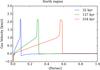 |
Fig. 9 Velocity field from numerical simulations for the northern H ii region expansion at three different times. Simulation is made with gravity and in an envelope of decreasing density, which is extrapolated from the observed one up to a constant density within rc = 0.005 pc. |
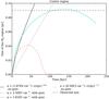 |
Fig. 10 Numerical simulations for the central UCH ii region expansion. In black: without gravity and in an envelope of decreasing density, which is extrapolated from the observed one up to a constant density within rc = 0.005 pc. In dotted black: without gravity in an envelope of decreasing density with a gradient typical of infall, ρ ∝ r-1.5. In cyan: with gravity and in an envelope with a constant density of 1.65 × 105 cm-3, just allowing the observed size to be reached (black dashed line). In dashed red: with gravity and in an envelope with a constant density of 2.5 × 105 cm-3, collapses again before reaching the observed size. |
4.2.2. Case of constant-density envelopes
We simulated the expansion in a constant density envelope, whose value could be compared to the initial average density of the envelope material swept up by the expansion. The latter is estimated through Eq. (4) (see Col. 2 of Table 4). This approach is validated in the case of the northern region (see Sect. 4.2.3) and is shown to be a good approximation for all H ii regions since, for analytical calculations without gravity, the expansion times given in Cols. 3 and 5 of Table 4 are similar.
The central UCH ii region and the western compact H ii region are quenched by gravity when densities approach the initial average density extrapolated from the observed envelope. For these two regions, we thus decreased the envelope average density until their H ii regions develop and reach their actual size. The associated expansion times are then upper limits measured for the densest, homogeneous, and constant density envelopes. Any density above this value would result in quenching or re-collapse before reaching the observed size. Any configuration that allows expansion up to the observed size leads to a shorter expansion time. The corresponding maximum values of the initial homogeneous constant density and expansion time are given in Cols. 7−8 of Table 4.
Figure 10 shows the effect of gravity on the expansion for the central UCH ii region in a constant low-density envelope (cyan curve) compared to the expansion in a decreasing density envelope constrained by observational data, but without gravity (black line). For higher density (red dashed curve), the re-collapse occurs, preventing the expansion to reach the observed size. The same re-collapse behaviour is observed for the western compact H ii region. At the beginning of the expansion, corresponding to small scales, gravity can have a strong influence. In the case of a constant-density envelope, the collected mass noticeably increases when size grows. The re-collapse of the shell is thus favoured in a constant-density envelope, but it occurs less easily in a more realistic, decreasing-density envelope or at larger size. At the beginning of the expansion, the expansion is faster, even with gravity, in the constant-density cases. This arises from the fact that the central density here is much lower than in the case without gravity of extrapolated envelopes with decreasing density. When the collected mass becomes important, the expansion is strongly slowed down by gravity and even stops. Re-collapse then occurs, at large distance, but a constant density is unrealistic for such large sizes.
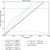 |
Fig. 11 Numerical simulations for the northern H ii region. Simulations with and without gravity are in colours and black, respectively. Continuous lines correspond to simulations with similar average initial density, ⟨ ρinitial ⟩ = 300 cm-3. The envelope has a decreasing power-law density with the characteristics of the observed one and extrapolated to a constant core of radius 0.005 pc (black) and 0.05 pc (dark blue). For the blue dashed line, the envelope has a power law decreasing density with an index corresponding to the observed gradient but with a 50 cm-3 density at 1 pc extrapolated to a constant core at 0.005 pc. For the cyan and red dashed curve, the envelope has a constant density of 300 cm-3 (cyan), corresponding to the average initial density, or a higher 2 × 104 cm-3 density (red dashed), leading to re-collapse. |
The northern H ii region could expand up to its observed size in an envelope with a maximum constant density of 5 × 103 cm-3. This density is much higher than the mean value extrapolated from observations, and the observed size would be reached in a very long and unlikely time of at least 3 × 10⁶ yr. At this large distance, re-collapse will not occur. More realistically, the northern H ii region should have expanded in an envelope with constant density of 300 cm-3 (cyan curve in Fig. 11), equal to the initial average density deduced from the envelope presently observed. This gives an expansion time of ~300 × 103 yr. As for the central UCH ii region, the constant-density envelope case has a low density at the centre. which favours the expansion at the beginning (cyan curve). But on large scales the expansion times of all models calculated for the nominal constant average density envelope converge to similar values. The same situation applies to the eastern H ii region. Better estimates of the expansion time can be obtained for the northern and eastern H ii regions, as shown in the Sect. 4.2.3.
4.2.3. Case of decreasing-density envelopes
The two options already mentioned in Sect. 4.2.1 for reducing the central density are suitable for the northern H ii region. The first option is to increase the radius of the constant density core, rc. The lower density and larger size of the northern region allows expansion with gravity without quenching up to the H ii region size. Nevertheless, the required size of the central core, rc ~ 0.05 pc (10 000 au), is then much larger than those inside which we expect a departure from the spherical symmetry (~0.001 pc/200 au−0.005 pc/1000 au). As in the case of a constant-density envelope, the initial conditions and the central structure of the H ii region has less of an impact on the analysis of the old and more developed northern H ii region since the expansion has already taken place for a longer time. This explains why the expansion times are not very different with and without gravity (blue and black continuous lines in Fig. 11). The highest central density allowing an H ii region expansion up to the observed size defines the maximum time of 370 × 103 yr (see Col. 9 of Table 4).
The second option is to lower the density of the overall structure, and in the northern H ii region case, a factor of two is necessary. The density thus decreased by 2, the expansion time is noticeably reduced as shown in Fig. 11 by the blue dashed line. From Eq. (9) (texp ∝ RStr− 3/4) and Eq. (6) (RStr ∝ ρ− 2/3), the expansion time relates to density through its square root: texp ∝ ρ1/2. This agrees with the time approximately divided by  between the two cases, ρ1 and ρ1/ 2 (blue and blue dashed lines in Fig. 11).
In fact the average initial density, ⟨ ρinitial ⟩, is identical for the three cases best representing the northern region. Case 1 is the first option mentioned above in this section with gravity and an enlarged central core (blue line), Case 2 is the simulation without gravity (black line), and Case 3 is for a constant density with gravity (cyan line). Regardless of whether the gravity is included in simulations, these three lines lead to similar expansion times. It indicates that the average initial density in which the H ii region has expanded is one of the important parameters for estimating expansion time. Once quenching by gravity has been overruled, the expansion is no longer strongly affected by gravity. In the details, however, the configuration with constant density and gravity underestimates the expansion time mainly in the central parts where the density should be much higher than what is estimated.
For the northern H ii region, expansion simulated in a decreasing envelope without gravity gives a minimum expansion time of 355 kyr. Expansion simulated with gravity in a decreasing-density envelope with the highest possible central density gives a maximum time of 370 kyr. These values define a very narrow interval for the expansion time, if extrapolation of the observed envelope towards the interior is valid. Taking the observational uncertainties into account, including those concerning the small scales structure, we conclude that the expansion time of the northern H ii region should be 350+/–50 kyr.
Even more strikingly, for the eastern H ii region, we do not need to increase the default central core radius (0.005 pc), and the time expansion calculated with gravity (24 kyr) is almost identical to the time obtained without gravity (23 kyr). This shows again that gravity could delay the start of expansion, but has very small influence on expansion time. This effect is more pronounced in a low-density medium.
4.2.4. Ionisation age and expansion time
Tracing the expansion of H ii regions with gravity and in a decreasing-density envelope extrapolated from the one observed at large scales would require complex 2D or even 3D configurations, at least on small scales. On large scales, in a decreasing-density envelope with a power law index q ≳ 1, once gravity has been overcome by turbulence and expansion occurs, the gravitational pressure decreases faster than the turbulent pressure, and its influence becomes negligible (Tremblin et al. 2014a, Sect. 5.1, Eq. (12)). Accretion within a rotating envelope can create a lower density zone where infall is driven from the envelope onto a disk or torus (see Tobin et al. 2008, Fig. 10; Hosokawa et al. 2010, Fig. 1; Ohashi et al. 2014, Fig. 5). The decreased density near the ionising objet reduces the influence of gravity. It should result in a reduction of the expansion time and decrease in re-collapse probability. Outflow lobes also modify the density structure and the geometry of the envelope (outflow cavity) and thus influence the expansion time. Infalling gas from the envelope itself locally increases the density and reduces the expansion speed or impedes it in a disk, torus, or funnel. All these effects, along with sporadic accretion (Peters et al. 2010a; Duarte-Cabral et al. 2013; De Pree et al. 2014), increase the expansion time uncertainty. A definitive measurement of the ionisation age would thus require a detailed modelling based on better constraints of physical parameters, at least on small scales. Unfortunately, the observational constraints of high-mass protostellar envelope on small scales (<0.05 pc) are still largely missing. This 3D small-scale asymmetric geometry could also shorten the quenching time, which needs to be added to the expansion time to determine the age of H ii regions and their ionising stars. On the other hand, confinement by external pressure could also occur at the end of expansion and thus lengthen the ionisation age. Expansion times depend on the initial conditions on small scales and especially ionisation age if the quenching and confinement times are taken into account. However, the order of magnitude of the expansion times determined from simulations seems to converge (see Table 4).
The simulations performed with or without gravity for the eastern and northern H ii regions expanding in low-density envelopes provide expansion times of 25 ± 5 × 10³ yr and 350 ± 50 × 103 yr. For the central UC and western compact H ii regions, we estimated upper and lower limits for the expansion time. Lower limits correspond to simulations in a decreasing-density envelope without gravity (Table 4, Col. 6). Upper limits are given by simulations with gravity in an envelope with the highest constant density (Table 4, Col. 8) avoiding quenching or re-collapse and allowing the observed size to be reached. The ranges of time values obtained, 90−150 ± 50 × 103 yr, are consistent with a mean expansion time of 1 × 10⁵ yr. The expansion time of the central UCH ii region, 9 × 10⁴ yr, agrees with the duration of the warm phase in dedicated chemical models (104–a few 105 yr, Treviño-Morales et al. 2014). The chemical model requires a chemistry out of equilibrium and imply a warm phase duration of less than 106 yr.
Despite the dependence on unknown small scale geometry, expansion times adopted for the dense western compact and central UCH ii regions are equal to within a factor two, converging to ~1−1.5 × 10⁵ yr (Table 4, Col. 10). They agree with the statistical estimate of the age of C and UCH ii regions (~105 yr, Wood & Churchwell 1989b) and are ten times longer than the rough dynamical time (~ 104 yr) estimated from the initial ionised gas velocity. As already stressed by Urquhart et al. (2013), the order of magnitude of these ages, 3−6 × 10⁵ yr, has recently been confirmed by new statistical lifetimes (~ 3 × 10⁵ yr, Mottram et al. 2011) and supported by a Galactic population synthesis analysis (2−4 × 10⁵ yr, Davies et al. 2011). The so-called lifetime problem (Wood & Churchwell 1989b; Churchwell 2002; Peters et al. 2010b) is simply solved here by taking an expansion velocity equal to the sound speed in ionised gas (cs) only at the beginning. Indeed, in a slowly decreasing-density envelope (q< 1.5) expansion speed is rapidly damped and even stopped if confinement by external turbulent pressure occurs (Raga et al. 2012).
4.3. Suitable approximations for expansion time estimation
As already mentioned in the previous section, gravity does not itself strongly affect the expansion time, but a delay of expansion can occur at the beginning. Similarly, Keto (2007) differentiates the dynamic behaviour of HC and UCH ii regions, which are gravitationally dominated, from that of larger compact and extended H ii regions, which are thermally dominated. As a matter of fact, in the low-density conditions of the northern and eastern regions, simulations with or without gravity give similar expansion times (see Table 4, Cols. 6 and 9). In the high-density condition of the central and western regions, the upper limit of expansion times calculated with gravity (Table 4, Col. 8), even with a rough constant density estimation, are only twice longer than expansion times obtained without gravity (Table 4, Col. 6).
Even if the average initial densities (⟨ ρinitial ⟩, Table 4, Col. 2) are only roughly estimated, expansion times of the various analytical calculations and simulations agree (Table 4, Cols. 3, 5, and 6). The agreement is better for the small (C and UC) H ii regions, for which the average initial density is more representative of the overall past density conditions. Analytical calculations without gravity using an extrapolation of the observed density envelope give a good time estimate at least for H ii regions of small sizes. For the more extended northern H ii region, the evaluation made of the average envelope density on small scales is more questionable since the remaining envelope has much lower density than the one at the beginning of expansion. Calculations using more realistically extrapolated density profiles should be preferred, or other evaluation using the pressure equilibrium and third Larson law (Tremblin et al. 2014a) could be made.
We conclude that:
-
Gravity induces quenching, which adds a delay before theH ii region expands, but when itexpands, the influence of gravity becomes marginal.
-
Envelope density profiles could be used to estimate a minimum expansion time from analytical calculations without gravity, and if density is not too high, it gives a realistic value.
-
The mean initial density is a good estimator of the matter density surrounding the massive protostar in early stages and is later collected in the shell by the H ii region expansion. It could be used to estimate expansion times if density profiles are not well defined. In any case, it is better suited to describe the intial density condition of ionisation expansion than the surrounding cloud density characterising the external medium.
All realistic time expansion estimates done in this paper converge around ~1 × 10⁵ yr for the two dense (UC central and compact western) H ii regions, ~2.5 × 10⁴ yr for the compact eastern H ii region, and ~3.5 × 10⁵ yr for the extended northern H ii region.
5. History of the formation of the B-type stars powering H II regions in Mon R2
In Sect. 5.1, we discuss the global infall of the Mon R2 cloud. In Sect. 5.2, we analyse the two-slope profiles in the framework of the inside-out collapse of envelopes and estimate protostellar infall ages. In Sect. 5.3, we compare the infall and ionisation ages and propose a full history of massive star formation in the Mon R2 cloud.
5.1. Cloud global infall
The density structure and infall kinematics discussed here are probably dominated by the most massive object clearly identified in Fig. 2b. The envelope profile defined above (see Sect. 3.5) and their corresponding values given in Table 3 have been used in Eq. (A.2) to estimate a mass of ~3500 M⊙ in a 2.5 pc radius for the central UCH ii region. This region exhibits a steeper density gradient in its outer envelope, with qout ≃ −2.5, also illustrated by the cloud structure studied with probability density function (Schneider et al. 2015; Rayner et al., in prep.). It suggests compression by external forces, as shown in numerical simulations of Hennebelle et al. (2003) and outlined in Appendix A. This compressive process could be associated with stellar winds and ionisation shocks of nearby stars such as those observed in the M 16 massive YSO (young stellar object) by Tremblin et al. (2014b) or with globally infalling gas driven by the dynamic formation of Mon R2 cloud through force fall. Such infalling motions have in fact been observed in CO by Loren (1977), and clumps with similar masses generally exhibit active global infall. This is the case of SDC335, which has a mass of ~5500 M⊙ in 2.5 pc (Peretto et al. 2013) and contains a protostellar object of similar type B1 (Avison et al. 2015), as well as of DR21, Clump-14 (DR21-south, ~4900 M⊙), and Clump-16 (DR21-north, ~3350 M⊙) (Schneider et al. 2010a), all of which show supersonic infall (V = 0.5−0.7 km s-1). Moreover, the hourglass morphology of the magnetic field is thought to be a signature of global infall (Carpenter & Hodapp 2008), and Koch et al. (2014) suggest that Mon R2 is a super critical, quickly collapsing cloud. The expected infall velocity gradient, as observed in SDC13 (Peretto et al. 2014), seems to be a crucial ingredient for generating the filament crossing (Dobashi et al. 2014) characteristic of all the regions mentioned here and commonly observed in many places.
5.2. Time elapsed since the beginning of the protostellar infall
The outer envelope of the two compact eastern and western H ii regions display a column density index of pout ≃ −1 ± 0.2, which corresponds to a ρ(r) ∝ r-2 density law. It recalls the density distribution of the singular isothermal sphere (SIS, Shu 1977) and that of the cloud structures quasi-statically forming clumps in numerical simulations with or without turbulence and magnetic field (e.g. Li & Shu 1996). A similar density distribution is in fact obtained for clumps forming from subsonic infall (Dalba & Stahler 2012) or supersonic flows (Gong & Ostriker 2009). This is also reminiscent of the density profiles found for low-mass and high-mass protostellar envelopes in early stages (Tsitali et al. 2013), which has been known for a long time (e.g. Motte & André 2001; Beuther et al. 2002). Numerous pre-main sequence phase YSOs are found in the Mon R2 cloud, suggesting that a group or cluster of protostars has most probably formed within the same area of these four separate envelopes of ~ 2.5−3 pc radius each.
The transition radius between the inner and outer envelopes, RInfall, could be used to locate the front of the infall expansion wave associated with the protostellar collapse. Indeed, in the case of an inside-out collapse developing into a static envelope with a SIS density structure, the envelope matter is free-falling as soon as the infall front wave travelling outwards reaches its location (e.g. Shu 1977). Interestingly, the density profile measured for the inner envelope surrounding H ii regions is close to that of free-falling material, ρ(r) ∝ r-1.5 (see Table 3). The transition radii would correspond to late stages of the protostellar collapse since they are rather large compared to typical protostellar envelopes: RInfall ~ 0.3, 0.5, 0.9, 2 pc versus Rprot ~ 0.03−0.1 pc (e.g. Motte & André 2001). This free-falling envelope material may not be able to reach the stars but may pile up at the periphery of the H ii regions, located at RH ii.
We assumed below that the infall front wave initiated at the time of the protostellar embryo formation and propagating outwards from the centre can be approximated by RInfall. The latter was measured to be 0.3, 0.5, and 0.9 pc for the central, western, and eastern ultra-compact and compact H ii region envelopes (see Table 3). We used an infall front-wave velocity equal to the isothermal sound speed, 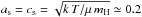 km s-1, calculated for T = 13.5 K, which is the mean cloud temperature in Mon R2. We then dated the beginning of the protostellar infall using the following equation:
 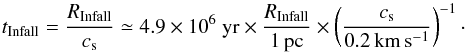 (11) It dates back to a few million years ago for the three compact and ultra-compact H ii regions with tInfall ≃ 1.5 × 10⁶ yr for the UCH ii and tInfall ~ 2.5−4.5 × 10⁶ yr for the eastern and western H ii regions. The more developed northern H ii region has an envelope that could be fully free-falling up to a radius reaching the background density (see Table 3). With a value of RInfall> 2 pc, our calculation leads to a minimum infall age of tInfall> 107 yr. These ages perhaps seem too long, but they are approximate values since a more complex density, temperature, and kinematic structure is to be expected for a non-isothermal envelope that is already globally collapsing at the time of the creation of the first protostellar embryo.
Moreover, the static SIS initial conditions are probably far from realistic, particularly for clouds forming high-mass stars, which are known to be dynamical entities (Schneider et al. 2010a; Peretto et al. 2013). Some models examined the protostellar collapse in an infalling cloud (Larson 1969; Penston 1969; Gong & Ostriker 2009; Keto et al. 2015). The initial inflow speed before protostellar collapse indeed modifies directly or indirectly the rarefaction wave speed, even in subsonic mode (Dalba & Stahler 2012). In the case of supersonic flows, the speed increases by a factor 2 to 3 (Gong & Ostriker 2009, see their Sect. 4.2), dividing the calculated infall time by the same factor. Supersonic inflows driven by the cloud’s global collapse, is probable for the central UCH ii region. It is less certain but still plausible for the other H ii regions, which are within the same infalling cloud but excentred from the infall centre.
Infall times are listed in Col. 6 of Table 3. The range of values illustrates systematics and errors to statistical uncertainties. All in all, it gives the following infall times: ~1. ± .7 × 106 yr for the central UCH ii region, ~1.5 ± 1. × 106 yr for the western CH ii region, and ~3. ± 1.5 × 10⁶ yr for the eastern CH ii region. Deducing the ionisation expansion time estimated in Sect. 4 from this infall time provides a measure of the time a protostar needs to reach the high-mass regime associated with the emission of ionising UV photons and an eventual ionisation delay due to quenching or swelling (Hoare & Franco 2007).
5.3. Age comparison and history of OB star formation in Mon R2
For the dense compact and ultra-compact (western and central) H ii regions, infall ages derived in Sect. 5.2: are about ten times greater than the ionisation expansion time tinfall ~ 1−2 × 10⁶ yr versus tionisation ~ 1−2 × 10⁵ yr. As for the eastern compact H ii region, the infall time is 100 times longer than the ionisation expansion time: tinfall ~ 3 × 10⁶ yr versus tionisation ~ 25 × 103 yr. The infall age of the northern extended H ii region is unknown with a lower limit of tinfall > 14 × 106 yr, which is ~30 times more than the ionisation expansion time of tionisation ~ 5 × 10⁵ yr. Even if uncertain, the order of magnitude of these values is probably realistic since the stellar ages of the B-type star association observed in Mon R2 is ~1−6 × 10⁶ yr (Herbst & Racine 1976; Carpenter et al. 1997), in agreement with the computed infall ages of the compact and ultra-compact H ii region envelopes.
Subtracting a mean protostellar lifetime of 3 × 10⁵ yr (Duarte-Cabral et al. 2013; see also Schisano et al. 2014, and references therein) from the infall time measured for the central UCH ii region, 1× 10⁶ yr suggests that ionisation started 7 × 10⁵ yr ago. With an ionisation expansion time of ~1 × 10⁵ yr, the quenching delay time could be ~6 ± 5 × 10⁵ yr. The typical protostellar lifetime adopted here agrees with the one obtained for the cold phase of Mon R2 in chemical models (105−106 yr, Treviño-Morales et al. 2014), corresponding to collapse (Esplugues et al. 2014). Similar considerations for western (and eastern) CH ii region give a quenching delay time of ~9 ± 6 × 10⁵ yr (resp. ~2 ± 1 × 10⁶ yr). These variations could be interpreted as an increase in the quenching time with increasing spectral type from B0 to B2.5, and thus decreasing number of ionising photons NLyc. However, given the large uncertainties of each of these estimates, a constant value around 106 yr cannot be ruled out.
Besides that, the derived infall ages span an order-of-magnitude difference, possibly indicating progressive star formation in the Mon R2 cloud. None of the ionisation fronts and none of the infall rarefaction wave arising from the three H ii regions located ~1–2 pc from the UCH ii region could, however, explain the compression of the UCH ii envelope. There is thus no clear evidence that star formation in the Mon R2 cloud could have been triggered by older local populations of stars. Any observed age gradient could only be related to sequential star formation triggered by an external agent.
6. Conclusions
We have presented a study of the Mon R2 molecular cloud based on dust column density and temperature maps built from Herschel/HOBYS observations and dedicated simuations. Our main findings can be summarised as follows:
-
1)
The MonR2 molecular cloud is dominated by gas associatedwith the central UCH ii region.The latter is located at the crossing of three major filaments, whilethree other H ii regions developin their surroundings. The spectral type of ionising stars asestimated from 21cm fluxes are in very good agreement withthose obtained from visual spectroscopy. They all are earlyB-type stars.
-
2)
The size of ionised regions is estimated by the heating of big grains (Fig. 2a) and small grains excitation through their 70 μm flux (Fig. 5), in the close surrounding of H ii regions, probably within the PDR. It ranges from ~0.1 pc for compact and UCH ii regions to ~0.8 pc for the most classical extended H ii region.
-
3)
The H ii regions are surrounded by large and rather dense neutral gas envelopes (Renv ~ 2−3 pc,
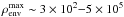 cm-3). At radii from ~0.1 pc to a few parsecs, the envelope surrounding H ii regions cannot be considered to have a constant density. Temperature gradients are also observed in the neutral gas envelope surrounding the four regions.
 -
4)
In spite of the quite advanced stage of evolution of the four massive ionising stars studied here, the density of the envelope surrounding them keep the imprint of earlier phases of the gravitational collapse. The density structure is similar to those expected for individual protostellar objects. For the first time the power law slope of the density profile is constrained accurately enough to distinguish between inner layers in free fall (ρ ∝ r− w with
 ) and external parts that could correspond to an equilibrium SIS configuration (ρ ∝ r-2).
 -
5)
We interpret the steep density profile of the central UCH ii region (ρ ∝ r-2.5) as due to an external pressure certainly associated with the observed global collapse, which can be called a forced fall.
-
6)
The transition radius between ρ ∝ r-1.5 (or r− w with
) and r-2 (or r− w with  ) laws should locate the free-fall rarefaction wave. Assuming it expands at one to three times the sound speed, we estimate the time since the infall began. An infall age around a few million years for these H ii regions is consistent with current high-mass star formation scenarios.
 -
7)
The density profiles obtained here allow us to determine the initial conditions of ionisation and its expansion. Dedicated 1D simulations show that the envelope density presently observed on a large scale would induce a complete quenching of the ionisation expansion. A more complex geometry on a small scale and a dynamic scenario are required to explain the present H ii region development.
-
8)
The ionisation expansion time deduced here from analytical calculations and dedicated simulations agree with statistical ages of the corresponding H ii region. The compact and UCH ii region expansion time is 1−2 × 10⁵ yr.
Stellar formation in MonR2 seems to be an on-going process that started at least ~1−6 × 10⁶ yr ago. Large scale feedback, such as the global infall of the cloud complex, certainly play an important role, but no clear evidence of locally triggered star formation has been found.
Online material
Appendix A: H II region expansion in an envelope of decreasing density with power law profile
Appendix A.1: Mass and average density from a decreasing power law density profile
When considering a decreasing density distribution described by a power law with an index q,  , the mass included within a radius R is given by
 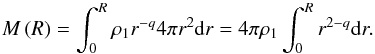 (A.1) As far as q< 3, it gives
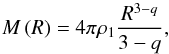 (A.2) or in numerical terms
 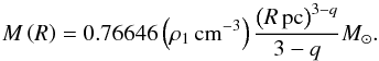 (A.3) The mean density in the sphere of radius R is then given by
 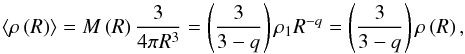 (A.4) and for a gradient typical of infall, q = 1.5, it gives
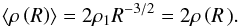
Appendix A.2: Ionisation expansion in a decreasing power law density profile
We consider here a decreasing density distribution with a power law of index q and a central core of constant density to avoid singularity at the origin and mimic a core envelope using the same definition as in Eq. (8): 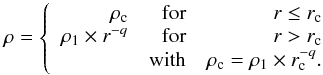 (A.5) Considering the density, ρi, and the speed, ci, in the ionised medium, the speed of the shell V, from the Rankine-Hugoniot conditions (Eq. (B.5), Minier et al. 2013) we get
 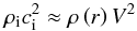 (A.6) using the density profile of (Eqs. (8)/(A.5)), it transforms into
 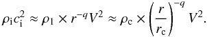 (A.7) Considering an initial Strömgren radius smaller than the core radius rc, Eq. (6) and the photon conservation gives
 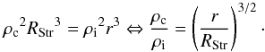 (A.8) Equation (A.7) can then be written as
 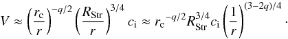 (A.9) This equation can be integrated to give the radius of the shell, rshell, as a function of time with tc the time at which the shell reaches rc:
 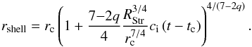 (A.10) Equation (A.9) taken at rc allows defining the speed at this point,
 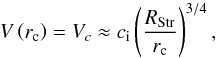 (A.11) and can be introduced in Eq. (A.10)
 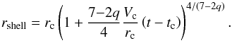 (A.12)
Appendix B: Column density line of sight calculation from an envelope of decreasing density with a power law profile
Column density dependance to power law index of decreasing density envelope.
When considering a decreasing density distribution with a power law of index q:, the column density as measured along the y axis at impact parameter a is given by 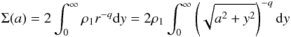 (B.1) with
  the column density at impact parameter a is then given by
  (B.2) The analytical integration for integer values of q leads to well-known integrals already calculated by Yun & Clemens (1991). Half integers lead to elliptical integrals, and their tabulated values result in a polynomial expression of
  . The analytical and numerical values are given in Cols. 2 and 3 of Table B.1. Adopting a value of 1 pc for the impact parameter a, we can derive a relation between the column density and the density via Σ1(a = 1 pc) = 2ρ1I(a = 1 pc). The relation of ρ1 as a function of Σ1 uses the conversion factor ζ corresponding to the appropriate q value and given in Col. 5 of Table B.1:
  (B.3) The dependence between ζ and q is given at the 5% error level by the following relation
  (B.4)
(B.4)
Appendix C: Density gradient steepening by external compression, as seen in simulations
Hennebelle et al. (2003) have made numerical simulations to test the influence on density profiles of compression induced by additional external pressure. The compression is characterised (see their Eq. (12)) by a dimensionless factor (φ) that gives the number of sound-crossing times needed to double the external pressure. High φ values correspond to low compression, called subsonic and slow pression increase. Hennebelle et al. (2003) show radial density and velocity profile at five time steps. The three first ones correspond to prestellar phases, well represented by Bonnor-Ebert spheres (Bonnor 1956; Ebert 1955). The fourth step would correspond to the protostellar class 0 phase and the last one to the beginning of the class I phase (see Andre et al. 2000 for classes 0 and I definitions). For a supersonic compression (φ< 1) during the prestellar phase, a density wave crosses the core profile towards the interior. For a sonic or subsonic compression ( ), the Bonnor-Ebert sphere like profile is smoothly distorted during prestellar phases leading to a single power law in protostellar phases.
Envelope density power law slope dependence on compression at two time step of protostellar stage.
We measured and give in Table C.1 the variation in the density profile power law index (q) as a function of the compression factor φ during the two time steps corresponding to the beginning and the end of Class 0 phase, (steps 4 and 5). During the Class 0 phase, the slope of the density profile does not depend on the compression and remains q = −2, the classical value expected for hydrostatic equilibrium. At the end of the Class 0 phase, the slope of the power law fitting the density profile is correlated to the compression given by the φ value (see Table C.1). It increases from 1.5, the classical value of a free-falling envelope, to 1.8 when φ varies from 10 (virtually no compression) to .1 (strongly supersonic compression). This 20% steepening of the density profile could be one effect that also occurs at a later stage and to larger radii as observed in the MonR2 central UCH ii region, as advocated in Sect. 5.2.
Appendix D: H II region swept-up shells and their contribution to the column density
The “collect-and-collapse” scenario proposes that the ionising flux of OB-type stars indeed efficiently sweeps up the gas located within the H ii region extent and develops a shell at the periphery of H ii bubbles (Elmegreen & Lada 1977).
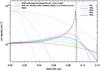 |
Fig. D.1 Contribution of the shell to the column density profile of the central UCH ii region. Its density radial extension is given by the two dashed black lines. The column density resulting from the line-of-sight accumulation is illustrated by the black solid line. The shell column density is then convolved with the Herschel beams (coloured dotted lines) to simulate the flux or column density of the shell (coloured solid lines) observable from 6″ (70 μm) to 36″ (500 μm) resolutions. |
We (see also Appendix E) investigate the contribution of this very narrow component to the column density measured with Herschel. This contribution should be especially large at the border of the H ii regions where the line of sight tangentially crosses the shell.
We thus chose to model the density structure of a shell surrounding an H ii region, similar to the one powered by the Mon R2-IRS1 star. We used a density structure that linearly increases with the radius, ρ(r) ∝ r (see Fig. 3) to mimic those suggested by the calculations of H ii region expansion (Hosokawa & Inutsuka 2005, 2006), giving more weight to the shell outer layers, and a thickness of ~0.002 pc as modelled by Pilleri et al. (2013, Fig. 2). Pilleri et al. (2012, 2013) studied the shell of the central Mon R2 UCH ii and considered two concentric slabs with homogeneous density, located at ~0.08 pc around the H ii region. In their model, the photo-dissociation region slab has a density of 2 × 105 cm-3 and a 6.5 × 10⁻⁴ pc thickness, while the high-density shell has a 3 × 106 cm-3 density and a 10-3 pc thickness. We used the densities of these slabs to model the inner and outer density values of the shell surrounding the central UCH ii region.
Figure D.1 shows the column density result of the central UCH ii shell calculated with the assumptions above, the idealised profile of this shell (black solid line), flat towards the centre and sharply increasing to the border. The shell was convolved with the Herschel beams (dotted coloured lines) to evaluate its contribution to the fluxes and column density profiles measured towards this H ii region. The border increase due to the shell seen tangentially is completely smeared out for all Herschel wavelengths tracing the cold gas density, i.e. for λ ≥ 160 μm (see Fig. D.1). The column density profiles measured by Herschel have angular resolutions that are too coarse (25″ and 36″), by factors of at least four. On top of that, the mixing along the line of sight with other density components, such as the envelope and background filaments, means that the centre-to-limb contrast of the shell is rarely observable. We thus cannot expect to resolve any shell around compact or ultra-compact H ii regions located at 830 pc. In contrast in the case of the extended northern H ii region, the relative contribution of the shell compared to the envelope is more important, increasing the centre-to-limb contrast and allowing a marginal detection of the shell (see Fig. 8). Therefore, the shell is not a dominant component of the column density structure of H ii regions and their surroundings, but it cannot always be neglected for its complete bubbling.
Appendix E: Column density dilution on the central line of sight by shell
Appendix E.1: Attenuation by shell in homogenous envelope
We first assumed the simple scenario of a bubble expanding in an homogenous envelope where which all the matter initially located within a sphere with a RH ii radius concentrates in the shell located at this very same radius. According to numerical simulations, the H ii region’s swept-up shells have small thicknesses, Lshell< 0.01 pc (e.g. Hosokawa & Inutsuka 2005). The almost total mass transfer from the bubble to the shell thus leads to the approximate equation, ![\appendix \setcounter{section}{5} \begin{eqnarray} \label{eq:ShellAndBubble} M_\text{initial} & =& \frac {4}{3}\pi\, {R_{\rm \ion{H}{ii}}}^3 \times \rho_\text{initial} \nonumber \\[3mm] & = & M_\text{shell} \simeq 4 \pi \, {R_{\rm \ion{H}{ii}}}^2 \,L_\text{shell} \times \rho_\text{shell}, \end{eqnarray}](/articles/aa/full_html/2015/12/aa26239-15/aa26239-15-eq407.png) (E.1) where ρinitial is the initial constant density of the envelope, and ρshell the shell density, assumed to be homogeneous. Using the relation between ρshell and ρinitial given by Eq. (E.1), the column density of the shell, Σshell, measured along the line of sight towards the centre of the region simply relates to that of the initial gas sphere, Σinitial(r<RH ii), with homogeneous density ρinitial and radius RH ii through
(E.1) where ρinitial is the initial constant density of the envelope, and ρshell the shell density, assumed to be homogeneous. Using the relation between ρshell and ρinitial given by Eq. (E.1), the column density of the shell, Σshell, measured along the line of sight towards the centre of the region simply relates to that of the initial gas sphere, Σinitial(r<RH ii), with homogeneous density ρinitial and radius RH ii through ![\appendix \setcounter{section}{5} \begin{eqnarray} \label{eq:colden} \Sigma_\text{shell} & = & \Sigma_\text{obs} = 2\times (L_\text{shell} \times \rho_\text{shell}) \nonumber \\[3mm] & \simeq & 2 \times (R_{\rm \ion{H}{ii}} \times \rho_\text{initial}\, /3) = \Sigma_\text{initial} \,/ 3 . \end{eqnarray}](/articles/aa/full_html/2015/12/aa26239-15/aa26239-15-eq412.png) (E.2) The column density measured towards the center of H ii regions with fully developed bubbles is thus expected to be divided by three compared to its original value:
(E.2) The column density measured towards the center of H ii regions with fully developed bubbles is thus expected to be divided by three compared to its original value: 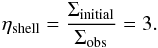 (E.3) When approaching the border of the H ii region, the line of sight crosses a greater part of the shell, and the column density reaches higher values. However, as shown in Appendix. D, the very small size expected for the shell will result in a beam dilution with very small enhancement that is usually not observable.
In the case of an H ii region of radius RH ii that not fully developed within an envelope of density ρinitial, to reach its external radius, Renv, the contribution of the outer residual envelope, Σenv, needs to be accounted for. The initial column density is now Σinitial(r<Renv) = 2 × Renv × ρinitial. The column density observed towards the developed H ii bubble would thus be ![\appendix \setcounter{section}{5} \begin{eqnarray} \Sigma_\text{obs} & = & \Sigma_\text{shell}+\Sigma_\text{env} \simeq \Sigma_\text{initial} \,/ 3\times \frac{R_{\rm \ion{H}{ii}}}{R_{\rm env}} + \Sigma_\text{initial}\times \frac{R_{\rm env} - R_{\rm \ion{H}{ii}}} {R_{\rm env}}\nonumber\\[3mm] & \simeq& \Sigma_\text{initial} \times \frac{3\times R_{\rm env} - 2 \times R_{\rm \ion{H}{ii}}} {3\times R_{\rm env}}, \end{eqnarray}](/articles/aa/full_html/2015/12/aa26239-15/aa26239-15-eq417.png) (E.4) and the decreasing factor or line-of-sight attenuation factor, η, would be
(E.4) and the decreasing factor or line-of-sight attenuation factor, η, would be 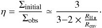 (E.5) It can be noticed that for a fully extended H ii region that reaches the size of the envelope RH ii = Renv, the attenuation factor reaches 3, the value already obtained for the shell alone.
These purely geometrical attenuation factors are weak for the small compact and ultra-compact H ii regions (η ≃ 1.1/1.2), but start to be noticeable for the more extended northern H ii region (η ≃ 1.5). We could estimated the density of the initial protostellar envelope before the H ii region develops, ρinitial, by correcting the mean density ⟨ ρobs ⟩, measured in Sect. 3.4.1 from observed column density through Eq. (3). The density correction due to the geometrical effect of H ii region expansion is obtained by the following relation: ρinitial ~ ⟨ ρobs ⟩ × η.
Appendix E.2: Attenuation in an envelope of decreasing density
In the more realistic case of an envelope with a decreasing density gradient, it is expected that the attenuation factor of the column density by H ii bubbles, η, should be greater than in the case of a constant-density envelope and constantly increasing as the H ii region expands.
The mass collected in the shell for the expansion of the H ii region at a radius RH ii is given by Eq. (A.2). The density in the shell of thichness Lshell is, then, 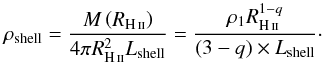 (E.6) The column density observed for this shell at small impact parameter, near the H ii region centre is then
 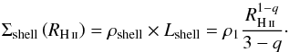 (E.7) The initial value of the column density was
 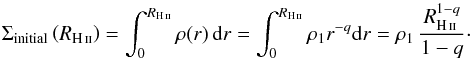 (E.8) This relation is valid only for q < 1 when the value of R1−q near 0 is negligible. The attenuation by the shell is given by
  (E.9) For constant density envelope (q = 0), Eq. (E.3) is recovered.
To evaluate the attenuation with an existing residual outer envelope we have to calculate the corresponding column density contribution,  (E.10) then
  will give, after some calculations,
 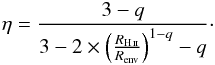 (E.11) For a shell reaching the size of the envelope RH ii = Renv, Eq. (E.11) leads to Eq. (E.9), which is obtained for the shell alone, and for a constant density envelope (q = 0) it gives Eq. (E.5)
These relations are only valid for q< 1, owing to the singularity at the origin of the density distribution.
Appendix E.3: Attenuation in envelope of decreasing density with a constant density core
To avoid the singularity at the origin we need to use the density profile defined by Eq. (A.5) with a central core of constant density ρc and a size of rc. Following the same calculation as above they give for the mass ![\appendix \setcounter{section}{5} \begin{eqnarray} \label{massDEWCC} M\left( R\right) & = & \int_{0}^{R} \rho \left( r \right) V \left( r \right) {\rm d}r \nonumber \\[4mm] & = & \int_{0}^{ r_\text{c}} \rho \left( r \right) V \left( r \right) {\rm d}r + \int_{r_\text{c}}^{R} \rho \left( r \right) V \left( r \right) {\rm d}r \nonumber \\[4mm] & = & \frac{4\pi \rho_1 R^{3-q} }{ 3 - q} \left( 1 - \frac{q}{ 3} \left( \frac{r_\text{c}}{R} \right)^{3-q} \right) , \end{eqnarray}](/articles/aa/full_html/2015/12/aa26239-15/aa26239-15-eq435.png) (E.12) the density in the shell
(E.12) the density in the shell 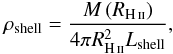 the shell column density near the centre of the H ii region
 ![\appendix \setcounter{section}{5} \begin{eqnarray} \label{coldensShellDEWCC} \Sigma_\text{shell} \left( R_{\rm \ion{H}{ii}} \right) & =& {\rho_\text{shell} } \times { L_\text{shell} } = \frac{M\left( R_{\rm \ion{H}{ii}} \right)}{4\pi R_{\rm \ion{H}{ii}}^{2} } \nonumber \\[4mm] & = & \frac{ \rho_1 R^{1-q} }{ 3 - q} \left( 1 - \frac{q}{ 3} \left( \frac{r_\text{c}}{R_{\rm \ion{H}{ii}}} \right)^{3-q} \right) , \end{eqnarray}](/articles/aa/full_html/2015/12/aa26239-15/aa26239-15-eq437.png) (E.13)
(E.13)
the initial value of the column density 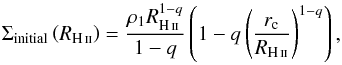 (E.14) and then the attenuation by the shell
 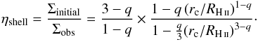 (E.15) All these relations reduces to the equivalent one of the previous section for rc = 0.
The same calculations as before for an existing residual outer envelope are still applicable here. As shown by Franco et al. (1990), the shell develops only for q< 1.5, so q< 3, and the terms  in the equations above are always negligible. Then the calculations give
  (E.16) for the attenuation, and for rc = 0 we recover Eq. (E.11)
The application to the northern H ii region with appropriate values of the different parameters gives an attenuation factor η ≃ 25, which becomes ~100 when the H ii region expansion reaches the size of the envelope (RH ii = Renv).
The formal treatment of the case of the compact and UCH ii regions would require considering an envelope with two density gradients, but the attenuation would be as efficient as for the northern extended H ii region once expansion of these region occurred.
Appendix F: Additional figures
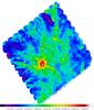 |
Fig. F.1 Column density map showing the azimuthal selection of areas used to characterise the density profiles of the eastern, western, and northern H ii region envelopes. The H ii region bubble, the inner, and the outer envelopes of the central UCH ii region are outlined with dashed circles, whose sizes are given in Tables 1−3. |
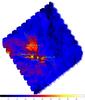 |
Fig. F.2 Hot regions overall contours of profile extraction on temp. map. Spectral type are taken from Racine (1968). |
NVSS : NRAO VLA Sky Survey, http://www.cv.nrao.edu/nvss/
The spectral types from Herbst & Racine (1976) were not used because they misidentified vdB 68 and vdB 69 (see Loren 1977, note 1) and because Racine (1968) used better spectral resolution.
The MonR2 IRAS fluxes donwloaded from Simbad (F12 = 470 Jy, F25 = 4100 Jy, F60 = 13 070 Jy, and F100 = 20 200 Jy) fulfil the Wood & Churchwell (1989a) and Kurtz et al. (1994) criteria: log (F25/F12) = 0.94 > 0.57, log (F60/F12) = 1.44 > 1.3, and F100 > 1000 Jy.
We used the relation by Bohlin et al. (1978) to transform Herschel NH2 measurements into AV values in mag unities, Av ≃ 1021 cm2 × NH2.
Available at http://irfu.cea.fr/Projets/Site_heracles
Acknowledgments
P.D. thanks Philippe Laurent for his help in calculating elliptical integral numerical values. This research has made use of TOPCAT (Taylor (2005), http://www.starlink.ac.uk/topcat/) and SAOImage/DS9, developed by the Smithsonian Astrophysical Observatory (http://hea-www.harvard.edu/RD/ds9/). This work profits from data downloaded from the SIMBAD database, operated at the CDS, and the VizieR catalogue access tool (CDS, Strasbourg, France; Ochsenbein et al. 2000). SPIRE was developed by a consortium of institutes led by Cardiff Univ. (UK) and including Univ. Lethbridge (Canada); NAOC (China); CEA, LAM (France); IFSI, Univ. Padua (Italy); IAC (Spain); Stockholm Observatory (Sweden); Imperial College London, RAL, UCL-MSSL, UKATC, Univ. Sussex (UK); Caltech, JPL, NHSC, Univ. Colorado (USA). This development has been supported by national funding agencies: CSA (Canada); NAOC (China); CEA, CNES, CNRS (France); ASI (Italy); MCINN (Spain); SNSB (Sweden); STFC (UK); and NASA (USA). PACS was developed by a consortium of institutes led by MPE (Germany) and including UVIE (Austria); KU Leuven, CSL, IMEC (Belgium); CEA, LAM (France); MPIA (Germany); INAF-IFSI/OAA/OAP/OAT, LENS, SISSA (Italy); IAC (Spain). This development has been supported by the funding agencies BMVIT (Austria), ESA-PRODEX (Belgium), CEA/CNES (France), DLR (Germany), ASI/INAF (Italy), and CICYT/MCYT (Spain). T.H. was supported by a CEA/Marie-Curie Eurotalents Fellowship. Part of this work was supported by the ANR (Agence Nationale pour la Recherche) project “PROBeS”, number ANR-08-BLAN-0241.
References
- Anderson, L. D., Zavagno, A., Deharveng, L., et al. 2012, A&A, 542, A10 [NASA ADS] [CrossRef] [EDP Sciences] [Google Scholar]
- Anderson, L. D., Deharveng, L., Zavagno, A., et al. 2015, ApJ, 800, 101 [NASA ADS] [CrossRef] [Google Scholar]
- Andre, P., Ward-Thompson, D., & Barsony, M. 2000, Protostars and Planets IV, 59 [Google Scholar]
- Arthur, S. J., Henney, W. J., Mellema, G., de Colle, F., & Vázquez-Semadeni, E. 2011, MNRAS, 414, 1747 [NASA ADS] [CrossRef] [Google Scholar]
- Aspin, C., & Walther, D. M. 1990, A&A, 235, 387 [NASA ADS] [Google Scholar]
- Avison, A., Peretto, N., Fuller, G. A., et al. 2015, A&A, 577, A30 [NASA ADS] [CrossRef] [EDP Sciences] [Google Scholar]
- Bacmann, A., André, P., Puget, J.-L., et al. 2000, A&A, 361, 555 [Google Scholar]
- Bernard, J.-P., Paradis, D., Marshall, D. J., et al. 2010, A&A, 518, L88 [NASA ADS] [CrossRef] [EDP Sciences] [Google Scholar]
- Beuther, H., Schilke, P., Menten, K. M., et al. 2002, ApJ, 566, 945 [NASA ADS] [CrossRef] [Google Scholar]
- Bohlin, R. C., Savage, B. D., & Drake, J. F. 1978, ApJ, 224, 132 [NASA ADS] [CrossRef] [Google Scholar]
- Bonnor, W. B. 1956, MNRAS, 116, 351 [CrossRef] [Google Scholar]
- Carmona, A., Pinte, C., Thi, W. F., et al. 2014, A&A, 567, A51 [NASA ADS] [CrossRef] [EDP Sciences] [Google Scholar]
- Carpenter, J. M., & Hodapp, K. W. 2008, The Monoceros R2 Molecular Cloud (Reipurth, B.), 899 [Google Scholar]
- Carpenter, J. M., Meyer, M. R., Dougados, C., Strom, S. E., & Hillenbrand, L. A. 1997, AJ, 114, 198 [NASA ADS] [CrossRef] [Google Scholar]
- Chini, R., Hoffmeister, V. H., Nielbock, M., et al. 2006, ApJ, 645, L61 [NASA ADS] [CrossRef] [Google Scholar]
- Churchwell, E. 2002, ARA&A, 40, 27 [Google Scholar]
- Churchwell, E., Watson, D. F., Povich, M. S., et al. 2007, ApJ, 670, 428 [NASA ADS] [CrossRef] [Google Scholar]
- Compiègne, M., Verstraete, L., Jones, A., et al. 2011, A&A, 525, A103 [NASA ADS] [CrossRef] [EDP Sciences] [Google Scholar]
- Condon, J. J., Cotton, W. D., Greisen, E. W., et al. 1998, AJ, 115, 1693 [NASA ADS] [CrossRef] [Google Scholar]
- Dalba, P. A., & Stahler, S. W. 2012, MNRAS, 425, 1591 [NASA ADS] [CrossRef] [Google Scholar]
- Davies, B., Hoare, M. G., Lumsden, S. L., et al. 2011, MNRAS, 416, 972 [NASA ADS] [CrossRef] [Google Scholar]
- de Gregorio-Monsalvo, I., Ménard, F., Dent, W., et al. 2013, A&A, 557, A133 [NASA ADS] [CrossRef] [EDP Sciences] [Google Scholar]
- De Pree, C. G., Peters, T., Mac Low, M.-M., et al. 2014, ApJ, 781, L36 [NASA ADS] [CrossRef] [Google Scholar]
- Deharveng, L., Zavagno, A., & Caplan, J. 2005, A&A, 433, 565 [NASA ADS] [CrossRef] [EDP Sciences] [Google Scholar]
- Deharveng, L., Zavagno, A., Anderson, L. D., et al. 2012, A&A, 546, A74 [NASA ADS] [CrossRef] [EDP Sciences] [Google Scholar]
- Dobashi, K., Matsumoto, T., Shimoikura, T., et al. 2014, ApJ, 797, 58 [NASA ADS] [CrossRef] [Google Scholar]
- Downes, D., Winnberg, A., Goss, W. M., & Johansson, L. E. B. 1975, A&A, 44, 243 [NASA ADS] [Google Scholar]
- Duarte-Cabral, A., Bontemps, S., Motte, F., et al. 2013, A&A, 558, A125 [NASA ADS] [CrossRef] [EDP Sciences] [Google Scholar]
- Dyson, J. E., & Williams, D. A. 1980, Physics of the interstellar medium (New York: Halsted Press), 204 [Google Scholar]
- Ebert, R. 1955, ZAp, 37, 217 [Google Scholar]
- Elmegreen, B. G., & Lada, C. J. 1977, ApJ, 214, 725 [NASA ADS] [CrossRef] [Google Scholar]
- Esplugues, G. B., Viti, S., Goicoechea, J. R., & Cernicharo, J. 2014, A&A, 567, A95 [NASA ADS] [CrossRef] [EDP Sciences] [Google Scholar]
- Franco, J., Tenorio-Tagle, G., & Bodenheimer, P. 1990, ApJ, 349, 126 [NASA ADS] [CrossRef] [Google Scholar]
- Fuente, A., Berné, O., Cernicharo, J., et al. 2010, A&A, 521, L23 [NASA ADS] [CrossRef] [EDP Sciences] [Google Scholar]
- Galliano, F., Hony, S., Bernard, J.-P., et al. 2011, A&A, 536, A88 [NASA ADS] [CrossRef] [EDP Sciences] [Google Scholar]
- Giannakopoulou, J., Mitchell, G. F., Hasegawa, T. I., Matthews, H. E., & Maillard, J.-P. 1997, ApJ, 487, 346 [NASA ADS] [CrossRef] [Google Scholar]
- Gong, H., & Ostriker, E. C. 2009, ApJ, 699, 230 [NASA ADS] [CrossRef] [Google Scholar]
- Gong, H., & Ostriker, E. C. 2013, ApJS, 204, 8 [NASA ADS] [CrossRef] [Google Scholar]
- González, M., Audit, E., & Huynh, P. 2007, A&A, 464, 429 [NASA ADS] [CrossRef] [EDP Sciences] [Google Scholar]
- Griffin, M. J., Abergel, A., Abreu, A., et al. 2010, A&A, 518, L3 [Google Scholar]
- Gutermuth, R. A., Pipher, J. L., Megeath, S. T., et al. 2011, ApJ, 739, 84 [NASA ADS] [CrossRef] [Google Scholar]
- Harsono, D., Jørgensen, J. K., van Dishoeck, E. F., et al. 2014, A&A, 562, A77 [NASA ADS] [CrossRef] [EDP Sciences] [Google Scholar]
- Hennebelle, P., Whitworth, A. P., Gladwin, P. P., & André, P. 2003, MNRAS, 340, 870 [Google Scholar]
- Henning, T., Chini, R., & Pfau, W. 1992, A&A, 263, 285 [NASA ADS] [Google Scholar]
- Herbst, W., & Racine, R. 1976, AJ, 81, 840 [NASA ADS] [CrossRef] [Google Scholar]
- Hildebrand, R. H. 1983, Quant. J. Roy. Astron. Soc., 24, 267 [Google Scholar]
- Hill, T., Pinte, C., Minier, V., Burton, M. G., & Cunningham, M. R. 2009, MNRAS, 392, 768 [NASA ADS] [CrossRef] [Google Scholar]
- Hill, T., Motte, F., Didelon, P., et al. 2011, A&A, 533, A94 [NASA ADS] [CrossRef] [EDP Sciences] [Google Scholar]
- Hill, T., Motte, F., Didelon, P., et al. 2012, A&A, 542, A114 [NASA ADS] [CrossRef] [EDP Sciences] [Google Scholar]
- Hindson, L., Thompson, M. A., Urquhart, J. S., et al. 2012, MNRAS, 421, 3418 [NASA ADS] [CrossRef] [Google Scholar]
- Hoare, M. G., & Franco, J. 2007, ArXiv eprints [arXiv:0711.4912H] [Google Scholar]
- Hosokawa, T., & Inutsuka, S.-I. 2005, ApJ, 623, 917 [NASA ADS] [CrossRef] [Google Scholar]
- Hosokawa, T., & Inutsuka, S.-I. 2006, ApJ, 646, 240 [NASA ADS] [CrossRef] [Google Scholar]
- Hosokawa, T., Yorke, H. W., & Omukai, K. 2010, ApJ, 721, 478 [NASA ADS] [CrossRef] [Google Scholar]
- Immer, K., Cyganowski, C., Reid, M. J., & Menten, K. M. 2014, A&A, 563, A39 [NASA ADS] [CrossRef] [EDP Sciences] [Google Scholar]
- Jaffe, D. T., Zhu, Q., Lacy, J. H., & Richter, M. 2003, ApJ, 596, 1053 [NASA ADS] [CrossRef] [Google Scholar]
- Jeffers, S. V., Min, M., Canovas, H., Rodenhuis, M., & Keller, C. U. 2014, A&A, 561, A23 [NASA ADS] [CrossRef] [EDP Sciences] [Google Scholar]
- Ji, W.-G., Zhou, J.-J., Esimbek, J., et al. 2012, A&A, 544, A39 [NASA ADS] [CrossRef] [EDP Sciences] [Google Scholar]
- Keto, E. 2007, ApJ, 666, 976 [NASA ADS] [CrossRef] [Google Scholar]
- Keto, E., Caselli, P., & Rawlings, J. 2015, MNRAS, 446, 3731 [NASA ADS] [CrossRef] [Google Scholar]
- Koch, P. M., Tang, Y.-W., Ho, P. T. P., et al. 2014, ApJ, 797, 99 [NASA ADS] [CrossRef] [Google Scholar]
- Kurtz, S., Churchwell, E., & Wood, D. O. S. 1994, ApJS, 91, 659 [NASA ADS] [CrossRef] [Google Scholar]
- Larson, R. B. 1969, MNRAS, 145, 271 [NASA ADS] [CrossRef] [Google Scholar]
- Li, Z.-Y., & Shu, F. H. 1996, ApJ, 472, 211 [NASA ADS] [CrossRef] [Google Scholar]
- Loren, R. B. 1977, ApJ, 215, 129 [CrossRef] [Google Scholar]
- Maret, S., Belloche, A., Maury, A. J., et al. 2014, A&A, 563, L1 [NASA ADS] [CrossRef] [EDP Sciences] [Google Scholar]
- Martín-Hernández, N. L., Vermeij, R., & van der Hulst, J. M. 2005, A&A, 433, 205 [NASA ADS] [CrossRef] [EDP Sciences] [Google Scholar]
- Massi, M., Felli, M., & Simon, M. 1985, A&A, 152, 387 [NASA ADS] [Google Scholar]
- Meyers-Rice, B. A., & Lada, C. J. 1991, ApJ, 368, 445 [NASA ADS] [CrossRef] [Google Scholar]
- Minier, V., Tremblin, P., Hill, T., et al. 2013, A&A, 550, A50 [NASA ADS] [CrossRef] [EDP Sciences] [Google Scholar]
- Motte, F., & André, P. 2001, A&A, 365, 440 [NASA ADS] [CrossRef] [EDP Sciences] [Google Scholar]
- Motte, F., Zavagno, A., Bontemps, S., et al. 2010, A&A, 518, L77 [NASA ADS] [CrossRef] [EDP Sciences] [Google Scholar]
- Motte, F., Bontemps, S., Hennemann, M., et al. 2012, in SF2A-2012: Proc. Annual meeting of the French Society of Astronomy and Astrophysics, eds. S. Boissier, P. de Laverny, N. Nardetto, et al., 45 [Google Scholar]
- Mottram, J. C., Hoare, M. G., Davies, B., et al. 2011, ApJ, 730, L33 [NASA ADS] [CrossRef] [Google Scholar]
- Mueller, K. E., Shirley, Y. L., Evans, II, N. J., & Jacobson, H. R. 2002, ApJS, 143, 469 [NASA ADS] [CrossRef] [Google Scholar]
- Nguyen-Luong, Q., Motte, F., Carlhoff, P., et al. 2013, ApJ, 775, 88 [NASA ADS] [CrossRef] [Google Scholar]
- Nielbock, M., Launhardt, R., Steinacker, J., et al. 2012, A&A, 547, A11 [NASA ADS] [CrossRef] [EDP Sciences] [Google Scholar]
- Ochsenbein, F., Bauer, P., & Marcout, J. 2000, A&AS, 143, 23 [NASA ADS] [CrossRef] [EDP Sciences] [Google Scholar]
- Ohashi, N., Saigo, K., Aso, Y., et al. 2014, ApJ, 796, 131 [NASA ADS] [CrossRef] [Google Scholar]
- Panagia, N. 1973, AJ, 78, 929 [NASA ADS] [CrossRef] [Google Scholar]
- Penston, M. V. 1969, MNRAS, 144, 425 [NASA ADS] [CrossRef] [Google Scholar]
- Peretto, N., Fuller, G. A., Duarte-Cabral, A., et al. 2013, A&A, 555, A112 [NASA ADS] [CrossRef] [EDP Sciences] [Google Scholar]
- Peretto, N., Fuller, G. A., André, P., et al. 2014, A&A, 561, A83 [NASA ADS] [CrossRef] [EDP Sciences] [Google Scholar]
- Peters, T., Banerjee, R., Klessen, R. S., et al. 2010a, ApJ, 711, 1017 [NASA ADS] [CrossRef] [Google Scholar]
- Peters, T., Mac Low, M.-M., Banerjee, R., Klessen, R. S., & Dullemond, C. P. 2010b, ApJ, 719, 831 [NASA ADS] [CrossRef] [Google Scholar]
- Pilbratt, G. L., Riedinger, J. R., Passvogel, T., et al. 2010, A&A, 518, L1 [CrossRef] [EDP Sciences] [Google Scholar]
- Pilleri, P., Fuente, A., Cernicharo, J., et al. 2012, A&A, 544, A110 [NASA ADS] [CrossRef] [EDP Sciences] [Google Scholar]
- Pilleri, P., Treviño-Morales, S., Fuente, A., et al. 2013, A&A, 554, A87 [NASA ADS] [CrossRef] [EDP Sciences] [Google Scholar]
- Pilleri, P., Fuente, A., Gerin, M., et al. 2014, A&A, 561, A69 [NASA ADS] [CrossRef] [EDP Sciences] [Google Scholar]
- Poglitsch, A., Waelkens, C., Geis, N., et al. 2010, A&A, 518, L2 [NASA ADS] [CrossRef] [EDP Sciences] [Google Scholar]
- Quireza, C., Rood, R. T., Bania, T. M., Balser, D. S., & Maciel, W. J. 2006, ApJ, 653, 1226 [NASA ADS] [CrossRef] [Google Scholar]
- Racine, R. 1968, AJ, 73, 233 [CrossRef] [Google Scholar]
- Raga, A. C., Cantó, J., & Rodríguez, L. F. 2012, MNRAS, 419, L39 [NASA ADS] [CrossRef] [Google Scholar]
- Richardson, K. J., White, G. J., Monteiro, T. S., & Hayashi, S. S. 1988, A&A, 198, 237 [NASA ADS] [Google Scholar]
- Roccatagliata, V., Preibisch, T., Ratzka, T., & Gaczkowski, B. 2013, A&A, 554, A6 [NASA ADS] [CrossRef] [EDP Sciences] [Google Scholar]
- Roussel, H. 2013, PASP, 125, 1126 [Google Scholar]
- Schisano, E., Rygl, K. L. J., Molinari, S., et al. 2014, ApJ, 791, 27 [NASA ADS] [CrossRef] [Google Scholar]
- Schneider, N., Csengeri, T., Bontemps, S., et al. 2010a, A&A, 520, A49 [NASA ADS] [CrossRef] [EDP Sciences] [Google Scholar]
- Schneider, N., Motte, F., Bontemps, S., et al. 2010b, A&A, 518, L83 [NASA ADS] [CrossRef] [EDP Sciences] [Google Scholar]
- Schneider, N., Bontemps, S., Simon, R., et al. 2011, A&A, 529, A1 [NASA ADS] [CrossRef] [EDP Sciences] [Google Scholar]
- Schneider, N., Bontemps, S., Girichidis, P., et al. 2015, ArXiv e-prints [arXiv:1507.08869] [Google Scholar]
- Shu, F. H. 1977, ApJ, 214, 488 [NASA ADS] [CrossRef] [Google Scholar]
- Shu, F. H., Lizano, S., Galli, D., Cantó, J., & Laughlin, G. 2002, ApJ, 580, 969 [NASA ADS] [CrossRef] [Google Scholar]
- Spitzer, L. 1978, Physical processes in the interstellar medium (New York: Wiley-Interscience) [Google Scholar]
- Strömgren, B. 1939, ApJ, 89, 526 [NASA ADS] [CrossRef] [Google Scholar]
- Strömgren, B. 1948, ApJ, 108, 242 [Google Scholar]
- Tang, X. D., Esimbek, J., Zhou, J. J., et al. 2013, A&A, 551, A28 [NASA ADS] [CrossRef] [EDP Sciences] [Google Scholar]
- Taylor, M. B. 2005, in Astronomical Data Analysis Software and Systems XIV, eds. P. Shopbell, M. Britton, & R. Ebert, ASP Conf. Ser., 347, 29 [Google Scholar]
- Thronson, Jr., H. A., Gatley, I., Harvey, P. M., Sellgren, K., & Werner, M. W. 1980, ApJ, 237, 66 [NASA ADS] [CrossRef] [Google Scholar]
- Tobin, J. J., Hartmann, L., Calvet, N., & D’Alessio, P. 2008, ApJ, 679, 1364 [NASA ADS] [CrossRef] [Google Scholar]
- Tremblin, P., Audit, E., Minier, V., Schmidt, W., & Schneider, N. 2012a, A&A, 546, A33 [NASA ADS] [CrossRef] [EDP Sciences] [Google Scholar]
- Tremblin, P., Audit, E., Minier, V., & Schneider, N. 2012b, A&A, 538, A31 [NASA ADS] [CrossRef] [EDP Sciences] [Google Scholar]
- Tremblin, P., Minier, V., Schneider, N., et al. 2013, A&A, 560, A19 [Google Scholar]
- Tremblin, P., Anderson, L. D., Didelon, P., et al. 2014a, A&A, 568, A4 [NASA ADS] [CrossRef] [EDP Sciences] [Google Scholar]
- Tremblin, P., Schneider, N., Minier, V., et al. 2014b, A&A, 564, A106 [NASA ADS] [CrossRef] [EDP Sciences] [Google Scholar]
- Treviño-Morales, S. P., Pilleri, P., Fuente, A., et al. 2014, A&A, 569, A19 [NASA ADS] [CrossRef] [EDP Sciences] [Google Scholar]
- Tsitali, A. E., Belloche, A., Commerçon, B., & Menten, K. M. 2013, A&A, 557, A98 [NASA ADS] [CrossRef] [EDP Sciences] [Google Scholar]
- Urquhart, J. S., Thompson, M. A., Moore, T. J. T., et al. 2013, MNRAS, 435, 400 [NASA ADS] [CrossRef] [Google Scholar]
- van den Bergh, S. 1966, AJ, 71, 990 [NASA ADS] [CrossRef] [Google Scholar]
- Walmsley, M. 1995, Rev. Mex. Astron. Astrofis., 27, 137 [Google Scholar]
- Whalen, D., & Norman, M. L. 2006, ApJS, 162, 281 [NASA ADS] [CrossRef] [Google Scholar]
- Wilson, B. A., Dame, T. M., Masheder, M. R. W., & Thaddeus, P. 2005, A&A, 430, 523 [NASA ADS] [CrossRef] [EDP Sciences] [Google Scholar]
- Wood, D. O. S., & Churchwell, E. 1989a, ApJ, 340, 265 [NASA ADS] [CrossRef] [Google Scholar]
- Wood, D. O. S., & Churchwell, E. 1989b, ApJS, 69, 831 [NASA ADS] [CrossRef] [Google Scholar]
- Xie, T., & Goldsmith, P. F. 1994, ApJ, 430, 252 [NASA ADS] [CrossRef] [Google Scholar]
- Yun, J. L., & Clemens, D. P. 1991, ApJ, 381, 474 [NASA ADS] [CrossRef] [Google Scholar]
- Zavagno, A., Russeil, D., Motte, F., et al. 2010, A&A, 518, L81 [NASA ADS] [CrossRef] [EDP Sciences] [Google Scholar]
- Zhu, Q.-F., Lacy, J. H., Jaffe, D. T., Richter, M. J., & Greathouse, T. K. 2005, ApJ, 631, 381 [NASA ADS] [CrossRef] [Google Scholar]
- Zhu, Q.-F., Lacy, J. H., Jaffe, D. T., Richter, M. J., & Greathouse, T. K. 2008, ApJS, 177, 584 [NASA ADS] [CrossRef] [Google Scholar]
All Tables
Comparison of the properties of the neutral envelopes surrounding the four H ii regions of Mon R2.
Envelope density power law slope dependence on compression at two time step of protostellar stage.
All Figures
|
Fig. 1 Three-colour Herschel image of the Mon R2 molecular complex using 70 μm (blue), 160 μm (green), and 250 μm (red) maps. The shortest wavelength (blue) reveals the hot dust associated with H ii regions and protostars. The longest wavelength (red) shows the cold, dense cloud structures, displaying a filament network. The dashed rectangle locates the four H ii region area shown in Fig. 2. |
| In the text | |
|
Fig. 2 Dust temperature (colours in a) and contours in b)) and column density (colours in b) and contours in a)) maps of the central part of the Mon R2 molecular cloud complex, covering the central, western, eastern, and northern H ii regions with 36″ resolution. The heating sources of H ii regions are indicated by a cross and with their name taken from Racine (1968) and Downes et al. (1975). Smoothed temperature and column density contours are 17.5, 18.5, and 21.5 K and 7 × 10²¹, 1.5 × 10²², 5 × 10²², and 1.8 × 1023 cm-2. |
| In the text | |
|
Fig. 3 H ii region and its surrounding four-component spherical model and radial profile of density (right). The ionised bubble is first surrounded by the shell containing all of the swept-up material. The neutral envelope is made of two parts with different density gradients finally merging into the background. The short dashed line represents the extrapolation of the inner envelope before the ionisation expansion and collecting process. |
| In the text | |
|
Fig. 4 Dust temperature radial profiles of the central UCH ii region showing a steep outer part and a flatter inner region. We note the agreement of the measurements done with the 3-band temperature map, T3B (red and magenta lines and points), and with the 4-band temperature map, T4B (yellow and pink lines and points). |
| In the text | |
|
Fig. 5 Radial intensity profiles of the central UCH ii region showing the measurements done at 70 μm (blue points) and 160 μm (green points) taking advantage of the PACS highest resolution, compared with the 3-band temperature (T3B) and the 4-band temperature (T4B) data given by the black arrow. The 160 μm profile decreases less in the inner part of the envelope (pink line) than in its outer part (yellow line). Since 160 μm emission is sensitive to dust temperature and density, this behaviour is probably related to the two different slopes found for the density profile of the envelope characterised in Sect. 3.4.1. The slope change indeed occurs at similar RInfall radius. |
| In the text | |
|
Fig. 6 H ii region bubble (yellow line and points) surrounded by a neutral gas envelope splitting into slowly and sharply decreasing NH2 parts (pink and blue lines and points). The background is defined by the lower limit of the clouds of grey points. The resolution corresponding to the Herschel beam at 500 μm is illustrated by the black curve in a). |
| In the text | |
|
Fig. 7 Column density profile of the central UCH ii region (cyan diamonds with σ errors bars) compared to models with all components illustrated in Fig. 3. The neutral envelope with two density gradients or with a single one are shown by a black line and a dotted black line respectively. An envelope model with a single density gradient cannot match the observed data. Individual components after convolution by the beam are shown by magenta, red, green, and blue dashed lines, for the bubble, shell, envelope and background. The continuous red line shows the unconvolved shell profile at an infinite resolution. |
| In the text | |
|
Fig. 8 Column density profile for northern H ii region and its four components coded with the same colours as in Fig. 7. The dotted green line corresponding to the sum of the envelope and background contributions matches well with observed data. |
| In the text | |
|
Fig. 9 Velocity field from numerical simulations for the northern H ii region expansion at three different times. Simulation is made with gravity and in an envelope of decreasing density, which is extrapolated from the observed one up to a constant density within rc = 0.005 pc. |
| In the text | |
|
Fig. 10 Numerical simulations for the central UCH ii region expansion. In black: without gravity and in an envelope of decreasing density, which is extrapolated from the observed one up to a constant density within rc = 0.005 pc. In dotted black: without gravity in an envelope of decreasing density with a gradient typical of infall, ρ ∝ r-1.5. In cyan: with gravity and in an envelope with a constant density of 1.65 × 105 cm-3, just allowing the observed size to be reached (black dashed line). In dashed red: with gravity and in an envelope with a constant density of 2.5 × 105 cm-3, collapses again before reaching the observed size. |
| In the text | |
|
Fig. 11 Numerical simulations for the northern H ii region. Simulations with and without gravity are in colours and black, respectively. Continuous lines correspond to simulations with similar average initial density, ⟨ ρinitial ⟩ = 300 cm-3. The envelope has a decreasing power-law density with the characteristics of the observed one and extrapolated to a constant core of radius 0.005 pc (black) and 0.05 pc (dark blue). For the blue dashed line, the envelope has a power law decreasing density with an index corresponding to the observed gradient but with a 50 cm-3 density at 1 pc extrapolated to a constant core at 0.005 pc. For the cyan and red dashed curve, the envelope has a constant density of 300 cm-3 (cyan), corresponding to the average initial density, or a higher 2 × 104 cm-3 density (red dashed), leading to re-collapse. |
| In the text | |
|
Fig. D.1 Contribution of the shell to the column density profile of the central UCH ii region. Its density radial extension is given by the two dashed black lines. The column density resulting from the line-of-sight accumulation is illustrated by the black solid line. The shell column density is then convolved with the Herschel beams (coloured dotted lines) to simulate the flux or column density of the shell (coloured solid lines) observable from 6″ (70 μm) to 36″ (500 μm) resolutions. |
| In the text | |
|
Fig. F.1 Column density map showing the azimuthal selection of areas used to characterise the density profiles of the eastern, western, and northern H ii region envelopes. The H ii region bubble, the inner, and the outer envelopes of the central UCH ii region are outlined with dashed circles, whose sizes are given in Tables 1−3. |
| In the text | |
|
Fig. F.2 Hot regions overall contours of profile extraction on temp. map. Spectral type are taken from Racine (1968). |
| In the text | |
Current usage metrics show cumulative count of Article Views (full-text article views including HTML views, PDF and ePub downloads, according to the available data) and Abstracts Views on Vision4Press platform.
Data correspond to usage on the plateform after 2015. The current usage metrics is available 48-96 hours after online publication and is updated daily on week days.
Initial download of the metrics may take a while.