| Issue |
A&A
Volume 583, November 2015
|
|
|---|---|---|
| Article Number | A118 | |
| Number of page(s) | 19 | |
| Section | Planets and planetary systems | |
| DOI | https://doi.org/10.1051/0004-6361/201525721 | |
| Published online | 03 November 2015 | |
Using the Sun to estimate Earth-like planet detection capabilities
VI. Simulation of granulation and supergranulation radial velocity and photometric time series
1
Université. Grenoble Alpes, IPAG,
38000
Grenoble,
France
e-mail:
This email address is being protected from spambots. You need JavaScript enabled to view it.
2
CNRS, IPAG, 38000
Grenoble,
France
3
Institut de Recherche en Astrophysique et Planétologie, Université
de Toulouse, 14 avenue Édouard
Belin, 31400, Toulouse, France
Received: 23 January 2015
Accepted: 31 July 2015
Abstract
Context. Stellar variability, at a variety of timescales, can strongly affect the ability to detect exoplanets, in particular when using radial velocity (RV) techniques. Accurately characterized solar variations are precious in this context to study the impact of stellar variations on planet detectability. Here we focus on the impact of small timescale variability.
Aims. The objective of this paper is to model realistic RV time series due to granulation and supergranulation and to study in greater detail the impact of granulation and supergranulation on RV times series in the solar case.
Methods. We have simulated a collection of granules and supergranules evolving in time to reproduce solar photometric and RV time series. Synthetic time series are built over the full hemisphere over one solar cycle.
Results. We obtain intensity and RV rms due to solar granulation of respectively 0.8 m/s and 67 ppm, with a strong variability at timescales up to more than 1 h. The rms RV due to supergranulation is between 0.28 and 1.12 m/s.
Conclusions. To minimize the effect of granulation, the best strategy is to split the observing time during the night into several periods instead of observing over a consecutive duration. However, the best strategy depends on the precise nature of the signal. The granulation RV remains large after even an hour of smoothing (about 0.4 m/s) while the supergranulation signal cannot be significantly reduced on such timescales: a reduction of a factor 2 in rms RV can for example be obtained over 7 nights (with 26 min/night). The activity RV variability dominates at larger timescales. Detection limits can easily be as high as 1 MEarth or above for periods of tens or hundreds of days. The impact on detection limits is therefore important and may prevent the detection of 1 MEarth planets for long orbital periods, while the impact is much smaller at small orbital periods. These results do not take the presence of pulsations into account.
Key words: techniques: radial velocities / planetary systems / Sun: activity / Sun: granulation / stars: activity / stars: solar-type
© ESO, 2015
1. Introduction
Stellar variability, at a variety of timescales, can strongly affect our ability to detect exoplanets. A systematic analysis of the radial velocity (RV) produced by active regions in the solar case has been done by Lagrange et al. (2010) and Meunier et al. (2010a). In these works, typical variability at timescales from one day to the cycle length has been studied. Three contributions to the RV variability have been considered: the spot intensity contrast, which affects the stellar RVs as the spot crosses the visible disk; the same process for bright plages; and the attenuation of the convective blueshift in active regions (plages being the dominant factor). We have shown that the resulting RV variations were strongly dominated by the third contribution, with timescales from the rotational period to the solar cycle length. The impact of the magnetic activity pattern on astrometry has also been estimated (Makarov et al. 2010; Lagrange et al. 2011).
Both RV and transit measurements are also affected by small-scale variability (minutes to hours). This has been studied for example by Aigrain et al. (2004), who derived photometric light curves, and by Dumusque et al. (2011b), who derived RV time series due to granulation or larger scale processes (supergranulation and the so-called mesogranulation) using the simple laws obtained by Harvey (1984) and later by Palle et al. (1995). The law for each component is, however, not very well constrained by the fits of observations. For example, Palle et al. (1995) show that the flat part of the solar RV spectrum due to granulation at low frequencies is much smaller than other contributions (supergranulation, activity) and is therefore not well constrained. Palle et al. (1995) have fitted four components (granulation, mesogranulation, supergranulation, and active regions) using the same law, but they observed that it was difficult to fit the timescale parameters and have therefore fixed them to the values derived by Harvey (1984). Because they fit the power spectrum with four components whose dependence on the frequency is fixed, it is mandatory to fit all four components with a significant amplitude otherwise there would be a gap, but it does not mean that these components are well fitted.
Lefebvre et al. (2008) have succeeded in fitting the photometric data obtained by GOLF/SoHO without the mesogranulation component. Furthermore, the very existence of mesogranulation has long been questioned (Straus et al. 1992; Rieutord et al. 2000). More recently, a number of works suggest that mesogranular scales are unlikely to be a true convective scale, the energy being injected at another scale (e.g., Yelles Chaouche et al. 2011; Berrilli et al. 2013). Nonetheless, it is possible that mesogranular flows are the consequence of a large-scale organization of granules (Roudier et al. 2009). Whether Harvey’s laws are adapted to mesogranulation is therefore not proved.
Several issues remain to be investigated: what is the contribution of granulation at larger timescales? Is the power spectrum flat, as expected from this description, or not? How would a time series derived from more precise properties of granules affect the sampling issues such as those discussed by Dumusque et al. (2011b)? What is the true contribution of supergranules, which is fitted by Palle et al. (1995) with a large power (rms RV of 1.9 m/s)?
We know that the law derived by Palle et al. (1995) can be reproduced with a simple simulation of a collection of a large number of cells with a typical size and lifetime, but it is important to take all parameters into account to simulate the produced RV or photometry and check whether the law is still valid at all timescales. Furthermore, such a law does not apply to activity.
It is therefore necessary to realistically model time series due to granulation and possibly to other contributions using a different approach in order to understand the true nature of the signal. Seleznyov et al. (2011) have simulated photometric time series due to granulation by considering a collection of granules evolving in time and by studying the resulting power spectrum. In this work, we follow a similar approach; we simulate photometric and RV variations due to a collection of cells. Contrary to the work of Seleznyov et al. (2011), however, we do not consider a fixed number of granules, but a fixed surface covered by the granules, because it allows us to consider the proper number of granules. We also take projection effects into account, which is necessary when dealing with RV, and simulate a full hemisphere, hence our simulation is more realistic. Our approach is complementary to that developed by Cegla et al. (2013) who reproduced spectra from different components in granules. It should also be noted that regarding granulation, although the root mean square (rms) RV and rms intensity I may be correlated (Cegla et al. 2014), such a correlation may be complex (Bastien et al. 2014); moreover, the two time series themselves are uncorrelated (see Sect. 3.2.1 for a discussion), therefore the photometric time series cannot be used to correct the RV time series due to granulation for example1.
Our approach is described in Sect. 2. We analyze our results in Sect. 3; we estimate the actual contribution of granulation at various temporal scales and the consequences on the analysis of RV time series when searching for exoplanets. Furthermore, we extend this work to the estimation of the contribution of supergranulation in Sect. 4. In Sect. 5 we use the simulation of Borgniet et al. (2015) to study the sum of the three contributions: granulation, supergranulation, and magnetic activity on RV and photometry, and discuss the contribution of mesoscale flows. Finally, the impact on planet detectability is studied in Sect. 6 using detection limits. We conclude in Sect. 7.
2. Description of the granulation simulation
2.1. Principle
We simulate a collection of granules spread over one solar hemisphere. Each of these granules is created by several processes with an initial size: granules are born either by appearance, from the merging of two nearby granules, or from a preexisting granule splitting into two parts. They then evolve in size with time, and finally either split into two granules, merge with a nearby granule, or disappear when their age has reached their lifetime. The total area covered by all granules at any time is equal to the hemisphere surface, i.e., we impose a fixed surface and not a fixed number of granules. Each granule is given a specific location on the surface. The star is considered to be non-rotating2, the lifetime of a granule being more than three orders of magnitude smaller than the rotation period. Finally, each granule is assigned a RV and an intensity (described in Sects. 2.4.1 and 2.4.2, respectively) according to its size and position (projection effects), which corresponds to the contribution of that granule to the integrated RV and intensity respectively. This allows us to build time series of RV and intensity variations due to granules.
At each time step, two situations are possible for each granule in the collection. If its current lifetime is lower than its attributed lifetime (described in Sect. 2.2.2), then its size evolved following the rule described in Sect. 2.2.1. If it has reached its theoretical lifetime, it will either disappear, merge with another granule, or split into two new granules (to which new properties will be assigned depending on the size of the fragments) as described in Sect. 2.2.3. This is done for all granules at each time step. A summary of the algorithm is presented in Sect. 2.3.
In the rest of this paper we assume that granular cells combined with intergranular lanes form the granules.
2.2. Physical parameters
2.2.1. Size parameters and size evolution
We use the size distribution observed by Roudier & Muller (1987). This distribution follows an exponential law, with a typical spatial scale of 1 Mm. We impose minimum and maximum sizes of 0.016 and 6.6 Mm2, respectively. This is also compatible with the results of Hirzberger et al. (1999) and Beeck et al. (2013). This distribution is shown in Fig. 1.
Granules are known to evolve during their lifetime. As in Seleznyov et al. (2011), who used the decay observed by Hirzberger et al. (1999), we take this evolution into account. We consider that granules below a typical size of 0.76 Mm2 linearly decrease in size during their lifetime while those that are larger linearly increase in size. The decay is chosen to linearly depend on the size, with a maximum value of 0.0145 Mm2/min; this value is smaller than the one used by Seleznyov et al. (2011) as large values lead to unrealistic size distributions.
2.2.2. Lifetime parameters
Hirzberger et al. (1999) have also shown that the lifetime depends on the size of granules. In this simulation we chose to attribute a lifetime to each granule according to its size following the law of Hirzberger et al. (1999), and to check afterward that the resulting distribution was indeed close to an exponential law with the proper timescale. The minimum lifetime considered is τmin = 1 min and the maximum lifetime τmax = 30 min. Because the published values (Hirzberger et al. 1999) provide mean sizes versus the lifetime without any precise value of the dispersion, we had to adapt these published values for our simulation. For sizes S below 2.4 Mm2, the lifetime follows the law τ = 1.5 + 4.375S to which a dispersion following a normal law with sigma = 2 τ/τmax minutes is added (corresponding to a dispersion of 0.07 min at τmin and of 2 min at τmax). For sizes S above 2.4 Mm2, the lifetime follows the law τ = 11.92 + 0.033S, to which a dispersion similar to the previous case is added, with the constraint that they must lie between the minimum and maximum values.
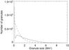 |
Fig. 1 Size distribution of granules from the exponential distribution from Roudier & Muller (1987) observed distribution (dashed line) and from the Rieutord et al. (2002) simulation (solid line). |
2.2.3. Birth and death of granules
Most granules appear from the splitting of a previsouly existing granule or from the merging of existing granules as shown by the observations of e.g. Oda (1984) and Hirzberger et al. (1999). Similarly, most observed granules also die either by splitting or by merging with other granules. The percentage of granules appearing or disappearing is small. It should be noted that there is no direct correspondence between the amount of birth by merging and the amount of death by merging because the splitting process can lead to more than two granules and merging can be done between more than two granules as well, but the proportions of the different configurations are not necessarily symmetric. In this paper, we consider merging between two granules only and fragmenting into two granules only, therefore our percentages are slightly different but still representative of observed granules.
Furthermore, Hirzberger et al. (1999) have shown that the birth and death processes depend on the size: small granules tend to be born by splitting while large granules result from merging. Similarly, small granules tend to die by merging while the largest ones die by splitting. This, as discussed for the size evolution of granules, also adds a significant complexity to the simulation if one wishes to reproduce the observed size and lifetime distribution. It is also time consuming: for each granule dying by merging, we need to search for the closest granule disappearing at the same time also by merging. In this paper we consider that granules below 0.76 Mm2 would most likely merge and that they would most likely fragment when larger. The transition between the two regimes is smoothed, typically over 2 Mm2, to avoid steps in the final distributions. At each time step, the list of granules at the end of their life is identified. Out of these, a percentage of granules (21%) is chosen to disappear directly, independent of their size (Hirzberger et al. 1999). The others follow the splitting/merging process. For the merging, the closest granules are considered, providing the sum of their two sizes is smaller than the maximum granule size. The birth of granules by merging and fragmenting is controlled by the death of previous granules. When a granule appears directly, its size is chosen so that the global distribution at this time step is as close as possible to the input distribution.
2.3. Summary: algorithm
The algorithm that creates granules can be summarized as follows:
-
Initialization. Granules are generated using the prescribed size distribution until they cover the full hemisphere (or prescribed surface for the small field-of-view simulations). Size-dependent properties are assigned to each of the n granules as they are created: lifetime, position on the disk, RV, intensity.
-
Loop over the time steps.
-
Loop over the n granules: Size modification according to their size.
-
Loop over the n granules: If their age has reached their expected lifetime, attribution of a status: disappearance, splitting, merging.
-
In the case of disappearance: the granule is eliminated from the list of granules.
-
In the case of splitting: the size of the two new granules is determined (each size being a fraction of the original granule size) as well as their new positions and properties (lifetime, RV, intensity).
-
In the case of merging: when the simulation covers the full hemisphere, large cells paving the whole surface are identified so that granules are grouped with other merging granules that are not far from each other to speed up the identification of granules merging with each other. For each of these cells, a loop over the merging granules is made: for each granule that has not already merged, the closest granule is identified and they merge. New properties (position, RV, intensity) are attributed to the new granule, whose size is the sum of their two parents’ sizes.
-
-
Update of the granule list and number n and computation of the surface coverage.
-
Addition of new granules until the hemisphere is completely covered. As in the initialization step, they are generated using the prescribed size distribution, but the procedure takes the size distribution of existing granules into account so that the total size distribution at each step follows as closely as possible the prescribed size distribution.
-
Computation of RV and intensity for each granule at this time step (see next section).
2.4. Velocity and intensity parameters
2.4.1. Velocity parameters
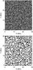 |
Fig. 2 Upper panel: intensity map from the convection simulation of Rieutord et al. (2002). Lower panel: segmentation showing identified granules. |
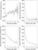 |
Fig. 3 Upper left panel: mean granule horizontal velocities (in one direction) over the cells |
In this section, we identify granules on maps produced by a hydrodynamical (HD) simulation (horizontal and vertical velocities, intensities) and derive their properties, which are used as inputs to our simulation. The RV contribution of granules is due to both horizontal and vertical velocity fields. Depending on the granule position on the disk, they contribute differently. The velocity is weighted with the local intensity. The vertical velocities result from the contributions of the velocity in the granular cells (upward flows) and in intergranular lanes (downward flows), of opposite signs. We used the convection simulation described in Rieutord et al. (2002) to extract granule contours and their velocity properties (Fig. 2). Two hundred maps of the velocity field (in the three directions) and intensity produced with a time step of 20 s were used for that purpose. Each image covers a field of view of 30 Mm × 30 Mm. We describe in Appendix A how the velocity properties of granules, shown in Fig. 3, are extracted. HD simulations do not include the effect of magnetic fields on the velocity fields, therefore the present parameters do not take the presence of magnetic fields into account even in the quiet Sun. The variation of the RV due to granulation affecting activity during the cycle is explored in Sect. 5.1.1.
2.4.2. Intensity parameters
Hirzberger et al. (1997) derived laws describing the evolution of the intensity inside granular cells and intergranular lanes, defined respectively as parts of the cell with intensity above and below average. We therefore extract the size of the intergranular lanes versus the granule size from the convection simulation. For each granule in our simulation, we first compute the area corresponding to the granular cell and the area corresponding to the intergranular lane using the law describing the half width of the intergranules δ = 0.22 + 0.02S for granules larger than 0.16 Mm2, otherwise δ is chosen to be equal to the radius of the granular cell. We then attribute an intensity to each area according to Hirzberger et al. (1997). The intensity in an intergranular lane pixel is equal to 0.98 to which a random dispersion following a normal law is added, with a dispersion of 0.1(1 − S/Smax). The intensity in a granular cell pixel is a size-dependant intensity to which a random dispersion following a normal law is added, with a dispersion of 0.2(1 − S/Smax). The size dependent intensity is chosen to be 1.03 for diameters d larger than 1.45 Mm and 0.95+0.055d for smaller cells. The two intensities are then weighted by the area covered by the bright (in granular cells) and dark areas (in intergranular lanes), to provide an intensity for that granule. A ponderation with a limb-darkening function is used in the full-disk simulations (Sect. 3.2 and later). As in Borgniet et al. (2015) we used the non-linear limb-darkening law from Claret & Hauschildt (2003), where the limb-darkening coefficients are the bolometric coefficients taken from ATLAS models (see Claret & Hauschildt 2003).
2.5. Simulation parameters
The time step must be small enough to produce realistic time series, hence it must be lower than the granule minimum lifetime. We found that a time step of 30 s gave good results (i.e., no artifact in the lifetime distribution). We have also compared these values with smaller time steps, 5 and 1 s, with almost no difference (see Sect. 3.1.1).
With such a small time step, long time-series simulations are time consuming. We have therefore performed two types of simulations:
-
Small field-of-view simulations: we performed several simulations covering the small field of view (30 Mm × 30 Mm) used in the convection simulation of Rieutord et al. (2002) for two purposes. First, we wish to estimate the impact of the projection effects and of some parameters on the results, and to compare different realizations. Second, we wish to make a comparison with the full convection simulation, covering 8 h with a few gaps. These simulations are analyzed in Sect. 3.1.
-
Full-disk simulations: we also performed simulations over the full hemisphere, corresponding to realistic conditions of stars. These simulations are analyzed in Sect. 3.2.
3. Granulation induced time series
3.1. Small field-of-view simulations
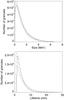 |
Fig. 4 Upper panel: snapshot size distribution of granules in the small field-of-view simulation #1 (solid line). The dashed line shows an exponential distribution with a typical size 1.01 Mm2 and the dot-dashed line an exponential distribution with a typical size of 1.29 Mm2. Lower panel: lifetime distribution of granules in the small field-of-view simulation #1 (solid line). The dashed line shows an exponential distribution with a typical scale of 3 min and the dot-dashed line an exponential distribution with a typical scale of 4.67 min. |
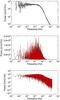 |
Fig. 5 Upper panel: smoothed power spectra (on a log scale) for ten realizations of the small field of view at disk center. Middle panel: original power spectrum (on a linear scale) for two of these realizations. Lower panel: same on a logarithmic scale. |
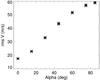 |
Fig. 6 Rms RV versus the position of the small field of view on the disk (α = 0 at disk center). |
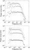 |
Fig. 7 Upper panel: smoothed power spectra for three categories of granule sizes in the small field-of-view simulation: granules smaller than 0.5 Mm2 (stars), granules between 0.5 and 1.5 Mm2 (diamonds), granules larger than 1.5 Mm2 (triangles). The solid line indicates the total power. Lower panel: same for the full-disk simulation. |
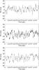 |
Fig. 8 Upper panel: zoom on a small field-of-view RV time series realized with a time step of 30 s. Middle panel: zoom on a small field-of-view RV time series realized with a time step of 5 s. Lower panel: extraction of 1 point every 30 s of the realization made with a time step of 5 s. |
3.1.1. Time series analysis
In this section, we study time series obtained for the small field of view over a 69-day period (200 000 time steps of 30 s). Figure 4 shows the size and lifetime distributions for a single realization of the time series. The size distribution shows a small deficit of very small granules compared to the exponential law, but as is seen in the next section the impact of this on the final RV is not significant. The final distribution corresponds to a size slightly larger than the typical size of 1.01 Mm2 corresponding to the input size distribution because of the evolution of granules. We find that the lifetime distribution corresponds to a typical lifetime of about three minutes. This is smaller than the six-minute lifetimes of Hirzberger et al. (1999), but it is not far from the results of Title et al. (1989) who obtained a typical lifetime of 2.53 min and from the results from the simulation of Beeck et al. (2013) with lifetimes between 2.6 and 4.1 min for example. The contribution of small granules from observations is very dependent on the quality of the observations. The impact of the size and lifetime distribution is discussed in the next section. The rms RV is 17.7 m/s and the rms I is 3125 ppm. Given the surface covered by the small field of view compared to the whole hemisphere, we could extrapolate that the full-disk rms RV should be on the order of 0.3 m/s. However, this final rms could be different if the projection effects are important (see Sect. 3.1.2).
Ten realizations of such time series have been performed. The power spectrum of these time series is shown in Fig. 5 (upper panel), showing that the impact of the dispersion on the power versus frequency is small at large frequencies. At low frequencies, the impact is naturally larger (the smoothing3 is made on a few points), but we note that these test simulations are performed over a short period of time. Figure 5 also shows two examples of unsmoothed power spectra, illustrating that the peaks that are visible in a given power spectrum are not indicative of a significant power at these precise periods, but instead are due to the specific realization.
3.1.2. Impact of projection effects
In a second step, we considered different positions of the small field of view on the disk to study the impact of projection effects. We note that the field of view always contains the same number of granules, but its projected surface becomes smaller as the angle α with the line of sight increases (α = 0 at disk center). Again, for each position, ten realizations are performed. The rms RV for each time series are shown in Fig. 6. The rms RV significantly increases toward the edge, suggesting that the rms RV for the full disk would be larger than the 0.3 m/s derived above. This increase occurs because the horizontal velocity amplitude in a granule is larger than the vertical velocities and because at the limb the line-of-sight velocities are dominated by the horizontal flows. Depending on α, the rms over the ten realizations is between 0.1 and 0.3 m/s. The impact of the projection effect on the intensity time series is, on the contrary, very small (and within the variation from one time series to the next), justifying the approximation made by Seleznyov et al. (2011) for this parameter, while it is crucial for a realistic RV simulation.
3.1.3. Impact of the different parameters
In this section, we test the impact of several of our parameters on the rms and power spectra.
Figure 7 shows the smoothed power spectra for three categories of granules: below 0.5 Mm2, between 0.5 and 1.5 Mm2, and above 1.5 Mm2. We find that, at least at disk center, large granules dominate the power spectrum.
We also investigate the impact of the time step used in the simulation. A zoom on our reference simulation is shown in Fig. 8 and is compared with a simulation made with a five-second time step. The variations are different since they correspond to different realizations of the granules, but we find that the variations are similar, and that the rms below 30 s is quite small. The rms RV are similar. Figure 9 shows the smoothed power spectra corresponding to these two simulations. For comparison purposes, we also interpolated the first series to get 5-s time steps and we extracted a 30-s time-step series from the 5-s time-step simulation. We find that the power spectra are very similar. The power obtained for the full 5-s time series is slightly lower than the other; when including more points at high frequency with lower level, the normalization of the power due to the Parseval’s Theorem becomes slightly different, as the sum of the power multiplied by the frequency bin is equal to the variance of the signal (which is constant). This shows that we can safely interpolate the 30-s time-step series to smaller time steps if necessary.
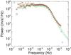 |
Fig. 9 Smoothed power spectra for several small field-of-view time series (disk center): simulation made with a 30-s time step for 200 000 steps (orange stars), the same simulation extrapolated every 5 s (blue crosses), simulation made with a 5-s time step for 1 200 000 steps (green squares), and extraction of 1 point every 6 points of this time series (red triangles). |
Small field-of-view rms RV.
Small field-of-view rms RV.
We now consider the evolution of the granules. In this paper, we took the merging and fragmenting of granules into account as well as their size evolution during their lifetime. The impact of this assumption is shown in Table 1. We find that the impact on the rms RV is very small, although there is a trend for slightly smaller rms RV when these effects are removed. Furthermore, removing the fragmenting and merging processes leads to a relatively larger rms at 1 h and 1 day, so this effect does not add any significant power at long timescales due to memory effects. Overall, these effects are very small. A comparison is also made with a white noise time series with similar rms, showing that the power at long timescales is significantly above what would be expected from white noise.
In Table 2, we summarize the impact of several granule properties on the results. We show that the assumption made in 2.4.1 for the vertical velocities in small granules is fully justified as the impact is very small (simulation 2). When increasing the size or the lifetime of granules, the rms are not modified significantly; however, the power at lower frequency (for example at 1 h or 1 day) increases.
3.1.4. Comparison with the convection simulation
In this section, we compare the RV time series obtained for the small field of view at disk center with that derived from the convection simulation made by Rieutord et al. (2002). We used the full time series of the convection simulation, covering a little more than eight hours, with a few gaps. Our small field-of-view simulation has been obtained with 20-s time steps for a more direct comparison.
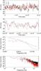 |
Fig. 10 First panel: RV time series for our small field-of-view simulation (black) and the convection simulation of Rieutord et al. (2002) (red). Second panel: zoom on the previous plot for a coverage of 5000 s. Third panel: smoothed power spectra for both time series. Fourth panel: same for the unsmoothed power spectra. |
The results are shown in Fig. 10. The rms RV is smaller in the convection simulation (11.3 m/s) than in our simulation (16.8 m/s) by about one-third. The uncertainties on our rms RV due to the realization are much smaller than this difference (about 0.1 m/s, see Sect. 3.1.1). It should also be noted that part of the convection simulation signal is also due to oscillations, which are not filtered out, so that the contribution of granules might be slightly smaller. We note that the oscillations should not significantly affect our choice of parameters because they are filtered out in Appendix A where we derive the velocities from the HD simulation. Finally, the size distribution is slightly different in both cases, but as is shown in Sect. 3.1.3, the contribution of small granules to the total power is small. Table 2 shows the results of a test in which we have truncated the size distribution below 0.5 Mm2 by imposing a constant number of granules below that size: we found a very small impact. The difference in amplitude could be due to the HD simulation not being as turbulent as the true Sun.
3.2. Full-disk time series and periodograms
3.2.1. Time series
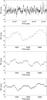 |
Fig. 11 First panel: 1-day zoom on a time series of granulation RV over the whole hemisphere, with a time step of 30 s. Second panel: same for a 1-h zoom. Third panel: 1-h zoom over a time series performed with a 5-s time step. Fourth panel: same for a 1-s time step. |
We have implemented a simulation of granules covering a full hemisphere over 12.5 years (to match solar cycle 23 and to be able to use the activity simulation over the same period), with time step of 30 s. We note that the properties derived from the HD simulation do not take the impact of magnetic field on granulation into account, but see Sect. 5.1.1 for a discussion. The resulting rms RV over the time series is 0.80 m/s and the rms photometry is 67 ppm. As pointed out in the introduction, our two time series in RV and photometry are uncorrelated. This seems to be different from what has been obtained by Cegla et al. (2015) using a completely different approach. Our interpretation is that with a realistic simulation involving on the order of 106 granules, although larger granules tend to have larger velocity fields and intensity contrasts, such a relationship between granule size and velocity and photometry properties is noisy: the sum of the contributions from all those granules therefore destroys any such correlation.
Figure 11 shows a zoom on this RV time series for a 1-day and 1-h period, respectively (two upper panels). We observe some variations at timescales significantly longer than a granule’s typical lifetime (a few minutes). This figure also shows 1-h zooms over similar simulations performed with smaller time steps. Our 30-s time step is indeed smaller than granule lifetimes, but not by a large factor: these two simulations therefore allow us to check the impact of this choice. The difference in rms RV and photometry is very small, on the order of 0.01–0.02 m/s and 1 ppm, respectively. The results for the three time steps are shown in Table 3.
We have also computed the RV time series for the different categories of granules. Granules smaller than 0.5 Mm2 (covering 5.4% of the surface) only contribute to 2.4% of the variance. Granules in the range 0.5–1.5 Mm2 (covering 29.4% of the surface) contribute to 28% of the variance. Granules larger than 1.5 Mm2 (covering 65.2% of the surface) contribute to 69.6% of the variance; therefore, there is a real effect of size: large granules contribute more than small granules. Two-thirds of the variation is due to granules larger than 1.5 Mm2. The uncertainties discussed in Appendix A for small granule properties therefore have a very small impact on the global time series. The power spectra for the different categories are shown in Fig. 7.
Full-disk rms RV.
3.2.2. Power spectra
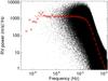 |
Fig. 12 Power spectrum of the RV granulation time series, for the full hemisphere and 30-s time step. The smoothed power spectrum is superimposed (red crosses), as is the fit by the function described in Sect. 3.2.2 (solid red line). |
The periodograms for the RV are shown in Fig. 12. Before smoothing, there is a very large dispersion in power at all scales, the position of the numerous peak depending on the realization. Figure 12 also shows a smoothed periodogram. The smoothed curves can be fitted with a function similar to that used by Harvey (1984) and Palle et al. (1995), 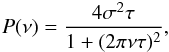 (1)with τ the timescale and σ related to the amplitude. A fit of the timescale gives 441 s (very similar to photometry), i.e., about 7.3 min, which is slightly smaller than the 472 s derived by Harvey (1984) and used by Palle et al. (1995), but on the same order of magnitude. The amplitude closely matches the amplitude observed by Palle 1995. The power starts to decrease at a few 10-4 Hz, which is compatible with Seleznyov et al. (2011), who found ~200 μHz for a 5.2 min granule lifetime. These results show that our approach is consistent with previous works.
3.2.3. Sampling issues: global dependence
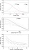 |
Fig. 13 Upper panel: rms of the smoothed granulation RV time series (red curve) versus scale. The rms RV of the corresponding residuals are in green. The horizontal dot-dashed line indicates a typical level of the noise induced by future instruments. Middle panel: rms RV of the granulation versus observing time during one night for a different number of observing periods n during each night (1: solid line; 2: dotted line; 3: dashed line; 4: dot-dashed line; 5: dot-dot-dot-dashed line). The exposure time is the observing time divided by n. Lower panel: same for the rms RV of the granulation versus the number of nights over which the signal is averaged, in the case of a 26-min observing time per night. |
The rms RV over the whole time span is 0.80 m/s, which is large compared to the instrumental noise expected from future instruments (below 0.1 m/s). It is therefore interesting to study how this rms decreases as the time series are smoothed out. We proceed as follows:
-
For a given timescale, we smooth the time series using a running mean.
-
We compute the rms RV of this smoothed time series.
-
We compute the residuals (RV times series minus the smoothed time series) and their rms RV for that scale: this shows the rms RV due to the signal at periods smaller than the considered scale.
Figure 13 shows the results for granulation. With a 1-h smoothing, the rms RV is still ~0.4 m/s (which is a much slower decrease than would be observed for white noise): this is comparable to the noise of current instruments or slightly below, but it is significantly higher than the noise of future instruments (0.1 m/s or less). It would require more than one night to reach a level of 0.1 m/s. This result also shows that averaging the RV signal due to granulation over timescales on the order of the cell lifetime (5–10 min) is not sufficient to decrease the rms significantly, as the rms RV decreases from 0.8 to 0.7 m/s in ten minutes: it is necessary to average the RV over a much longer timescale to observe a significant reduction of the rms RV.
Dumusque et al. (2011b) claimed that averaging granulation over 30 min averages out4: our results show that at this timescale, the rms RV is still on the order of 0.5 m/s for granulation alone.
3.2.4. Short-term temporal sampling and observing strategy
Since it is difficult to average out granulation, it is important to study the best observational strategy. Such an attempt has been performed by Dumusque et al. (2011b) for a simulation of several stars, using laws such as Harvey (1984) for granulation, mesogranulation, and supergranulation. Here, we consider a given observing time available during each 10-h night. This observing time is spread over the night in n observing periods (n between 1 and 5), providing an exposure time equal to the observing time divided by n.
The computations are made for a 1-year time series extracted from the whole time series and the results are shown in Fig. 13. Each curve in the middle panel corresponds to one strategy (i.e., a value of n). The best strategy is obtained when the observing time is spread over five observing periods, while the worst result is obtained for two observing periods. This is mostly true when little observing time is available: the trend for longer observing times is that the rms RV are very close to each other for the different strategies. After a 1-h averaging, the rms RV are, for example, in the range 0.3-0.4 m/s. They reach values below 0.2 m/s after at least eight hours of averaging.
We have also considered the case in which only a fraction of the given observing time is available (duty cycle) with measurements taken at random times during each observing period. The impact is very small, down to the 14% efficiency tested here: the dominant factor is therefore the duration of the observation over which the RV is averaged.
Finally, we consider the averaging over several nights. The result is shown in the lower panel of Fig. 13 in the case of 26 min of observing time per night. The trends are similar, with a rms RV reaching values below 0.1 m/s for the best strategy after a 6-night average. The best results are also obtained for a large number of observations during the night.
4. Supergranulation induced simulated time series
In this section, we perform a similar simulation for supergranules, as their contribution might be comparable to that of granules, although on different typical timescales. They last longer (typically 1.8 days instead of a few minutes), their size is much larger but they have much smaller velocity fields (hundreds of m/s instead of a few km s-1, but see the review of Rieutord & Rincon 2010).
4.1. Simulation parameters
The principle and algorithm of the simulation are similar to the granule simulation described in Sect. 2, i.e., we consider a collection of supergranules covering all of the visible hemisphere. Each supergranule contributes to the total RV and intensity. We adapt the parameters as follows:
-
Size distribution. Several authors have derived the size distribution of supergranules (Srikanth et al. 2000; Meunier et al. 2007c). Here we use the size distribution of Meunier et al. (2007c). For this simulation, we have fitted their cell radius distribution with an asymmetric law, with a mean of 9.392 Mm, a dispersion of 8.01 Mm, and an asymmetry factor of 2.55. The minimum and maximum radii are respectively 3 and 40 Mm.
-
Lifetimes. According to Del Moro (2004) supergranule lifetimes follow an exponential law with a typical scale of 22 h. However, the authors have also shown that supergranule lifetimes depend on their size. Here we use the following laws, derived from their analysis. We generate a typical timescale λτ for each diameter D, defined by −489+88.9D min for radius below 14 Mm, and 33 h for cells with a larger radius. For a given size, we then generate a timescale by using an exponential law that uses the proper λτ. We impose a minimum and maximum lifetime of 500 min (16.6 h) and 7000 min (117 h), respectively.
-
Evolution of supergranules: size, appearance, and disappearance. These parameters are not well constrained. In this paper we consider that supergranules appear or die in a similar way to granules, and we use the same percentages of the various categories and a typical radius threshold of 15 Mm between merging and fragmentation. No growing is considered.
-
Horizontal velocities. The contribution of the horizontal flows inside a given supergranule to the total RV is unfortunately not well constrained in the literature. Meunier et al. (2007c) showed that the rms inside a cell was larger for the largest cells, with a typical amplitude of ~33 m/s for the largest cells, and ~6 m/s for the smallest. They have also estimated the typical radial (horizontal) flows inside a cell (average horizontal velocity versus the position in the cell) and found typical velocities of about 200 m/s, with larger velocities for the largest cells. For our simulation we want to know the horizontal velocity (in one direction) averaged over the cell as a function of the size. One way to estimate at least an order of magnitude would be to scale the supergranule behavior from the granule laws. This is risky because, for example, the rms velocity inside a granule is about two times smaller than the typical horizontal flow, while in supergranules it is one order of magnitude smaller. Keeping this in mind, such a scaling based on the horizontal velocities rms provides 6 m/s for the largest cells and 31 m/s for the smallest cells. A scaling based on the typical horizontal velocities gives values that are four times larger. The uncertainty is therefore very large (a factor of 4 on the amplitude). In this paper we build simulations using the lower bound values and provide the upper limit by multiplying the RV by 4. We expect the true values to be between these two extrema.
-
Vertical velocities. Vertical velocities in supergranules are much weaker than horizontal flows. We scale them to the horizontal flows according to Hathaway et al. (2002). The ratio between the two components depends on the size. We use the ratio 10−0.5−0.373LogR.
-
Intensities. Meunier et al. (2007b) have shown that intensity variations inside supergranules, after eliminating the magnetic field contribution, is small and corresponds to a temperature variation on the order of 1 K between the centers of the cells. Furthermore, no significant variations with the cell size could be derived. Hence in our simulation we consider a constant intensity. Taking into account the variations due to the network would be possible, using the work of Meunier et al. (2007a,b) providing relationships between the magnetic field amplitude, the position in the supergranule cells for various size ranges, and intensity. As this corresponds to the network contribution and since we also model the activity contribution using a completely different modeling (Borgniet et al. 2015), we do not consider this variation here. The velocities are, however, weighted by the same center-to-limb darkening as for granulation (Claret & Hauschildt 2003).
The simulation is performed with a time step of 30 s to make the comparison with granulation easier (although a larger time step, typically 250 s, would be enough to contain all the information, given the typical lifetimes) over 12.5 years (length of solar cycle 23) to be consistent with our previous simulation and allows us to analyze the RV time series over the same long timescales.
4.2. Times series
An example of the RV variations due to supergranulation is shown in Fig. 14 on two different timescales (50 days and 1 day). Large variations on the order of 1 m/s and 0.3 m/s are observed at these timescales. When using the lower values of the estimated velocity field and taking into account fragmentation and merging as for granules, we obtain a rms RV of 0.28 m/s over our whole time series. The upper limit would correspond to a rms RV of 1.12 m/s. These values are therefore in the same range as the granule rms RV (0.8 m/s). The true value is probably between these extremes.
Palle et al. (1995) have fitted a 1.9 m/s rms RV to their data, significantly above our upper limit. However, as pointed out above, the fact that they fix the timescale constrains the amplitude, and therefore this amplitude is not entirely reliable. This value is much higher than our upper limit, and we consider it unlikely that solar supergranule properties allow for such a large rms.
We have tested the impact of the evolution of supergranules, and found very little difference when merging and fragmentation are suppressed; the impact is therefore extremely small compared to our uncertainty on the velocity field.
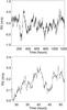 |
Fig. 14 Upper panel: 50-day time series of supergranulation RV, for the low velocity field assumption. Lower panel: the same over 1 day. |
4.3. Power spectra
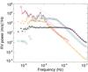 |
Fig. 15 Smoothed power spectrum of the RV granulation time series, for the full hemisphere and 30-s time steps (black stars), fitted by the Harvey function (black solid line). The power spectrum for supergranulation (minimum values) is shown with orange diamonds, the activity signal with red triangles, and mesogranulaion derived from supergranulation scaled to the Palle et al. (1995) parameters with blue squares. The green solid line corresponds to the sum of the three contributions (granulation, minimum supergranulation, activity) and the pink solid line is the same, but includes the maximum supergranulation. The green and pink dashed lines include mesogranulation. The black dotted line indicates the level fitted by Palle et al. (1995). The activity signal is cut above 30 min due to our time step. |
Figure 15 shows the smoothed power spectrum due to supergranulation (minimum value) superimposed on the granulation spectrum. The fit by the function defined in Sect. 3.2.2 gives a timescale of 33 h. The amplitude is smaller than that derived by Palle et al. (1995), as already derived from the rms RV in Sect. 4.2.
4.4. Sampling issues
As we did for granulation, we also studied the variation of the rms RV when smoothing the supergranulation time series. This is shown in Fig. 16. The two left columns show supergranulation alone (with our lower and higher limit). We find that smoothing the data over a realistic duration during the night does not decrease the rms RV significantly. Only a smoothing over several nights would allow that, and even a 5-day smoothing still gives a large rms RV (0.17 m/s for the minimum values). The last two columns show the same result when superimposing the granulation and the supergranulation RV time series. With the lower limit of supergranulation the rms are dominated by granulation, while they are strongly affected by supergranulation when using the higher limit.
The strategy in terms of number of observing periods during the night for a given observing time is similar for supergranulation and granulation alone, the rms RV is decreased more efficiently by splitting the available observing time into several periods during the night (the largest number of periods we tested was 5). When superimposing the two components, the best strategy seems to be 4 periods, especially when using the high limit for supergranulation. This strategy does not greatly affect the average over several nights. The rms strongly decreases with an increasing number of nights, reaching 0.15 m/s for 10 nights, with the lower level of supergranulation alone. For 10 nights, when combining the two signals, the rms is between 0.1 and 0.5 m/s, depending on the supergranulation level.
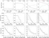 |
Fig. 16 First column: same as Fig. 13, for the lower limit of supergranulation. The exposure time is the observing time divided by n. Second column: same as Fig. 13, for the higher limit of supergranulation. Third column: same as Fig. 13, for the lower limit of supergranulation superimposed on granulation. Fourth column: same as Fig. 13, for the higher limit of supergranulation superimposed on granulation. |
5. Combined time series including granulation, supergranulation, and other contributions
5.1. Magnetic activity
It is interesting to add our granulation and supergranulation time series to the RV variations due to magnetic activity as modeled by Borgniet et al. (2015), since the contribution to the RV signal at large timescales is important, as shown by Lagrange et al. (2010) and Meunier et al. (2010a). Therefore, we combine the three time series together to study the total impact on the signal. As we know that magnetic activity affects granulation (as observed by the variable convective blueshift over the cycle), the velocity field associated with each granule is also expected to change when the granule is localized in an active region; we also estimate the impact of magnetic activity on the granulation time series themselves.
5.1.1. Approaches
We use a simulation of the RV due to solar activity derived by Borgniet et al. (2015) for the Sun. The contributions are due to spots, plages, and attenuation of convection in plages (Meunier et al. 2010b); however, these simulations were performed using a 1-day time step. In this paper we concentrate on small timescales, therefore several modifications have been introduced: a smaller time step is possible (in the present case 30 min), a small growing phase for spots and plages is introduced, the RV are computed directly from the list of structures without computing the spectra, and the RV results from the combination of the contributions from all the structures.
This time series is also used to build a corrected granulation time series Vcor. The attenuation of the convective blueshift taken into account in the activity simulation corresponds to an attenuation of two-thirds of the granulation signal over a certain fraction f of the surface (in plages and network). We therefore reduce the dispersion of the RV granulation time series V described in Sect. 3.2 according to this amplitude and the filling factor at any given time during the cycle: 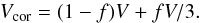 The resulting corrected granulation time series has a rms RV of 0.79 m/s over the whole time span, which is not significantly different from 0.8 m/s. The impact of convection attenuation, although very important on the global RV signal, is therefore very small on the small-scale dispersion.
We note that this simple computation does not take the rotation modulation into account. We only estimate the mean impact on the granulation RV dispersion due to the fact that a certain fraction of the granules are affected by the presence of magnetic activity. Indeed, we do not associate each granule directly with an active region, therefore the possible variability of the rms depending on the position of the affected granules on the disk is not accounted for. As the average effect is very small, we consider that a more precise computation would not significantly affect the corrected rms RV.
5.1.2. Power spectra
Figure 15 shows the power spectra due to activity superimposed on the granulation and supergranulation RV. It shows that the function used to fit the granulation or the supergranulation power is not adapted to the activity RV power spectrum (presence of the rotational modulation, different slope at medium frequencies). The amplitude of supergranulation and activity component is also smaller than that derived by Palle et al. (1995), while the granulation component is in very good agreement, perhaps because the observations cannot reliably constrain the parameters of activity and supergranulation given the short frequency domains available.
When considering the global power, compared to the observations of Palle et al. (1995) there is a lack of power typically in the range 10-6−10-5 Hz, corresponding to the mesoscale flows, which are not modeled in our work. It is not straightforward to model mesoscale flows as we modeled granulation and supergranulation because the origin is different and cells cannot be defined as precisely. To implement a realistic model of mesoscale flows is therefore outside the scope of the present paper. A simple approach is adopted in the next section.
5.2. Mesoscale flows
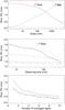 |
Fig. 17 Same as Fig. 13, for the lower limit of supergranulation added to granulation and a simple estimate of mesoscale flows. The exposure time is the observing time divided by n. |
We can however make a simple estimate of the impact of the presence of such an additionnal component by scaling the supergranulation time series to mesoscale flow properties, both in amplitude and temporal scale. The amplitude is changed to a 1.6 m/s rms (Palle et al. 1995) and the temporal scaling to τ = 1e4 s (Harvey 1984). The results are shown in Fig. 17. The strategy is not significantly affected, although the rms RV after averaging is even more difficult to reduce. For example, with the lower limit for supergranulation, the rms RV decreases from 1.83 m/s to 1.6 m/s only after a 1-h averaging, and 1 m/s after 10 h.
6. Impact on planet detectability
6.1. Sampling and method
In this section we investigate the impact of the granulation and supergranulation RV on planet detectability in detail. For simplicity, computations are made using a median amplitude for supergranulation, i.e., 2.5 times the lower amplitude (see Sect. 4.1). We complete this analysis by considering the sum of granulation, supergranulation, and mesoscale flows, magnetic activity alone, and the sum of the four components.
We consider the temporal samplings already used by Lagrange et al. (2010) and Meunier et al. (2010a). We introduce a four-month gap every year to simulate the impossibility of observing a given star all year. Then we consider four samplings: 1 measurement every day (1-day sampling, 2976 points over 12.5 years), every 4 days (4-day sampling, 732 points), every 8 days (8-day sampling, 372 points), or every 20 days (20-day sampling, 148 points). In addition, we also test a random sampling: a given number (20 or 40) of observing nights is considered each year and randomly allocated over eight months, which leads to 240- and 480-point time series covering 12 years.
For each of these samplings, the measurement is computed as follows. We choose one observing duration (30 min, 1 h, or 2 h) and we split it into five observing periods covering the whole night, as this was the best configuration derived in the previous section. The exposure time of each visit is then the total observing duration divided by five. The average over these five visits is then computed. Additionally, for the 8- and 20-day samplings, we also consider the average of similar measurements over 2 nights and 5 nights.
In each case, the new time series RV, hereafter RVstell, is analyzed as follows:
-
In Sect. 6.2, we compute periodograms of the RVstell. We compare them to the periodogram of RVpla due to a 1 MEarth planet at different semimajor axes and therefore different periods and for different phases and to the periodogram of RVstell + RVpla. Periodogram are computed using a Lomb-Scargle method and the power is in arbitrary units: the powers corresponding to the same sampling can be compared to each other.
-
In Sect. 6.3, we compute detection limits for the same planet periods. Detection limits are obtained using the LPA method (Meunier et al. 2012), a local method which takes the power into account in a window [0.75P–1.25P] where P is the considered period.
6.2. Periodograms
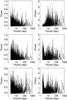 |
Fig. 18 Upper panels: periodogram of the granulation (left) and supergranulation with a level 2.5 times the minimum (right) time series for the 1-day sampling. The observation duration is 30 min split into 5 observing periods over one night. Middle panels: the same for half of the time series (1 point out of 2 is used, corresponding to a 2-day sampling). Bottom panels: the same for the other half. |
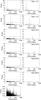 |
Fig. 19 First six rows: periodograms of the granulation RVstell + RVpla (left) and planet RVpla alone (right), for the 8-day sampling (30 min over 1 night). Each row corresponds to a different planet period from 3 to 480 days. The planet has a mass of 1 MEarth and an arbitrary phase. The false alarm probability at the 1% (dot-dashed lines) and 0.1% (dashed lines) levels are shown on the left plots. Last row: periodogram for the granulation RVstell alone. |
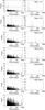 |
Fig. 20 As in Fig. 19 for supergranulation, for a level 2.5 times the minimum. |
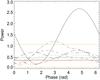 |
Fig. 21 Power at 480 d in the periodogram of the supergranulation + planet RV versus the phase of the planet (black lines). The supergranulation RV is obtained with the 8-day sampling, 30 min over 1 night. The planet has a period of 480 days and a mass of 1 MEarth. The power is the maximum for periods within 5% of the planet period. The different curves correspond to six different realizations of the time series for this sampling. The red curves correspond to the planet alone (same realizations). The green horizontal line is the average power for supergranulation alone, while the two orange horizontal lines indicate the minimum and maximum values of the power at 480 days for supergranulation alone (over the six realizations). |
Figure 18 shows an example of periodograms for the granulation and supergranulation RV and the 1-day sampling. In both cases a forest of peaks is present. Some of them can be quite high: see for example the peak just above a period of 100 days in the granulation periodogram. However, if we split each time series into two independant series, although the envelope of the peaks is similar from one series to the other, the exact positions of the largest peaks are completely different. It is therefore important to be careful of this effect when analyzing data as these RV do produce large peaks.
We now add a 1 MEarth planet to each series. Six periods are considered in the following: 3 d, 12 d, 50 d, 100 d, 300 d, and 480 d (the last corresponds to a planet at 1.2 AU as in our previous work). With these samplings it is increasingly more difficult to obtain a planet peak well above the granulation or supergranulation power.
We illustrate this with the 8-day sampling as it shows all configurations. Figure 19 (Fig. 20, respectively) shows the periodogram for the granulation (supergranulation) RVstell alone, for the planet RVpla alone (with an arbitrary phase) and for the combined RVstell + RVpla. For the granulation simulation, the planet peak is always distinguishable, although for the largest periods (300 and 480 days) its amplitude is similar to low period peaks in the granulation forest. Conversely, for supergranulation, for which the forest of peaks tends to extend toward larger periods, the planet peak is above the other peaks for periods up to 50 days only, while for the three largest periods the planet peak cannot be distinguished from the supergranulation power at all. Such a level of supergranulation RV should therefore prevent the detection of Earth mass planets in the habitable zone around solar-type stars on this 8-day sampling, even with no magnetic activity because it dominates the signal.
Figures 19 and 20 also show the usual false alarm probability (i.e., the probability that a peak of that amplitude is due to noise; hereafter fap) for each time series (granulation for supergranulation added to the planetary RV), for 1% and 0.1% probabilities. The planet peak is above the fap when the planet period is below 50 days (below 12 days, respectively) for granulation (supergranulation), while it is below the fap for periods above 100 days (50 days). Figure 19 also shows in some cases (at 300 and 480 days) a planetary peak that is well separated from the granulation signal and that can be clearly identified although it is below the fap, showing that the fap is not always a sufficient criterion.
We have shown a few examples of the planet peaks for a given realization and planet phase. Figure 21 illustrates the strong impact of these conditions on the power. We consider six slightly different realizations of the time series for the 8-day sampling and 30 min over 1 night in the case of supergranulation. For each of them we compute the power at the planet period (here 480 days) versus the phase of the planet. When the planet is alone, the peak is extremely stable, as shown by the red curves. However, when added to the supergranulation time series, the amplitude of the power at the planet period varies very strongly with the planet phase. It is also extremely sensitive to the realization. This is also true for supergranulation alone, as the power in the 480-day domain also varies significantly from one realization to the other. We note that all these simulations are made with no instrumental noise.
6.3. Detection limits
We now compute the detection limits for the same planet periods using the LPA method (Sect. 6.1). The peak at the planet period P is compared to the power of peaks around it (in our case within [0.75P–1.25P]) and not to all peaks in the periodogram. We use this method because the usual fap method does not give the same information: it tells us whether a peak has a certain level of significance (if all the signal were white noise), while we also want to know if a (planet) peak can indeed be distinguished from the rest of the signal (which is not white noise). A selection of these detection limits is shown in Fig. 22 and illustrates the impact of the sampling and averaging strategy. For all our tests and samplings, the granulation-only detection limits (first line in Fig. 22) are below 1 MEarth. They can however be close to 1 MEarth in a few cases, which means that when combined with other sources of noise a detection limit above 1 MEarth can very easily be reached, especially for long planet periods. As expected, the detection limit increases as the sampling is degraded from 1 day to 20 days, and decreases when the observing duration increases (over one night or by averaging over several nights).
In case of supergranulation (second line of Fig. 22), the trends are similar, but there is one main difference: averaging between 30 min and 2 h does not affect the detection limits, which is expected as this is a long timescale signal. However the amplitude is much larger: we obtain detection limits above 1 MEarth for the longest periods. For a period of 480 days for example, even two hours of observations per night averaged over 5 nights (i.e., 10 h of observing time) provide a detection limit around 1 MEarth.
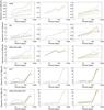 |
Fig. 22 First row: detection limits for granulation. The left panel shows the detection limit versus the planet period for a 30 min observing duration over 1 night, for different samplings: 1 day (red), 4 days (green), 8 days (orange), 20 day (blue), random sampling of 20 days per year (dashed yellow), random sampling of 40 days per year (dashed black). The middle panel shows the detection limit for the 1 day sampling over one night for different observing durations: 30 min (red), 1 h (green), 2 h (orange). The right panel shows the detection limit for the 8 day sampling over one night for different observing durations (same colors as middle panel) and nights: 1 night (solid lines), 2 nights (dashed lines), 5 nights (dotted lines). In all cases the horizontal dotted-dashed line shows the 1 MEarth level. Second row: same for supergranulation (at a level 2.5 times the minimum). Third row: same for granulation + supergranulation + mesogranulation. Fourth row: same for magnetic activity. Fifth row: same for the four components. |
When combining the granulation and supergranulation RV with the mesoscale flows RV (third line in Fig. 22), the trends are similar, but the detection limits reach the 1 MEarth limit at lower periods, from a few days (for the worse sampling) to ~40 days (for the best ones).
Finally, the detection limits including magnetic activity (fourth line for magnetic activity alone and fifth line for a combination of the four RV) are shown to illustrate the relative amplitude of the various components (which would be smaller if some corrections were applied). They are much larger because magnetic activity without correction dominates the signal. They are also much less sensitive to the strategy (observating duration, splitting into periods, averaging over several night) and are mostly sensitive to the sampling (with detection limits below 1 MEarth for the 1-day sampling at very small periods only).
We note that at short periods (below 12 days), the detection limit can be below 1 MEarth even when combining all components, but this requires a very good sampling (1 day over a long period).
Finally, we have also studied two random samplings with 240 and 480 points over 12 years. The results are shown in Fig. 22 (first column, yellow and black curves, respectively). They show similar trends. The detection limits are not strictly correlated with the number of points in the series, however, but this is probably related to the uncertainties on the detection limits (the detection limits are computed for only one realization of our time series).
7. Conclusion
We have developed a simulation of granulation photometric and RV time series covering a full solar cycle based on a collection of granules covering a solar hemisphere. We have extended this simulation to supergranulation and considered the combination of these signals with magnetic activity and mesogranulation. Our approach is complementary to that developed by Cegla et al. (2013) from MHD simulations of granulation, as we simulate long time series based on granulation photometric and velocity properties. We have obtained the following results:
-
The photometric rms due to solar granulation is 67 ppm and the rms RV is 0.8 m/s. The rms RV after a temporal smoothing of one hour remains large (0.4 m/s) and is significantly above the noise level of future instruments.
-
The smoothed power spectra of RV and intensity granulation time series is compatible with the fits made by Harvey (1984) or Palle et al. (1995); however, the power spectra before smoothing show many peaks.
-
Supergranulation, with a rms RV between 0.28 and 1.12 m/s depending on the assumption, has a rms RV comparable to the rms RV induced by granulation, and lower than the signal derived by Palle et al. (1995). It cannot be averaged out over one night however. After ten nights the signal still has a rms between 0.1 and 0.5 m/s depending on the assumption.
-
The best observational strategy is usually to spread the given observing time into several periods during the night (up to five have been tested), which is compatible with the results obtained by Dumusque et al. (2011a). However, the most efficient strategy seems to be dependent on the precise properties of the signal.
-
The impact of magnetic activity at timescales below 2–3 days is small compared to the other contributions (it is above the other contributions for periods larger than 6 days). Its impact on the rms RV due to granulation is also extremely small. Magnetic activity, therefore, should not significantly affect the detection of planets at very small periods, but must be considered for orbital periods above a few days. We note that pulsations are not taken into account and would also affect the best strategy.
-
A realistic modeling of mesoscale flows is beyond the scope of this paper as the origin of these flows is not well known. Its contribution is far from being well understood or well observed. A simple estimate shows that it contributes significantly to the RV signal, but that its impact on the observation strategy is not very different from the case with only granulation and supergranulation. After a significant averaging and considering the three components in the best case (granulation, mesogranulation, lower limit for supergranulation), the rms RV after 10 days is still ~0.5 m/s.
-
The presence of granulation or supergranulation has a significant impact on detection limits. Although their impact is smaller than the impact of magnetic activity, the detection limits due to granulation or supergranulation alone can easily increase to 1 MEarth in the habitable zone for observations spread over a 12.5-year interval. The main contribution comes from supergranulation. Contrary to magnetic activity for which there are possibilities to correct at least for part of their contribution to RV, it is difficult to correct for the granulation or supergranulation RV given their stochastic nature, as it is not possible to use the photometric signal, for example. One way is to average the signal, and its efficiency is limited due to the intrinsic nature of the signal (unless one observes stars with a lower level of convection, as in later spectral-type stars). Another way might be to use complementary information extracted from the spectra such as the line profiles or cross-correlation function on the spectra like in Cegla et al. (2015). Such sophisticated approaches would most likely need very high signal-to-noise spectra to be implemented.
When considering a collection of stars, the rms RV and I tend to be correlated (Aigrain et al. 2012; Haywood et al. 2014; Cegla et al. 2014) because large granules tend to produce larger velocity and have a larger contrast in intensity. However, for a given star we find that the time series of RV and I due to granulation are not correlated with each other, while the relationship between the two in the case of magnetic activity may make it possible to correct for the activity components (Aigrain et al. 2012; Haywood et al. 2014).
As stellar rotation broadens observed line profiles, the resulting RV may differ slightly from one star to the other depending on the rotation rate, an effect which cannot be taken into account in our simulation. The timescale of supergranulation, considered in Sect. 4, is also larger than for granulation.
The smoothing consists of averaging over bins with a constant size in Log(frequency) of ~0.083.
They do not quantify this reduction as they provide rms RV for all processes and not granulation alone: a direct comparison is not possible as we consider different stars, but for α Cen A, for example, which is a G2V-type star with an original rms RV in their synthetic series of 1.89 m/s – but only 0.4 m/s due to granulation – they find that for an averaging of 30 min they get a rms RV around 1.2 m/s for a single observation and around 0.8 m/s for three observations separated by 2 h.
The dispersion of this normal distribution is chosen to be 1025.47-574.449S+152.957S2-17.6675S3+0.720379S4 m/s.
Acknowledgments
Most of the computations presented in this paper were performed using the CIMENT infrastructure (https://ciment.ujf-grenoble.fr), which is supported by the Rhône-Alpes region (GRANT CPER07_13 CIRA: http://www.ci-ra.org). We are very grateful to Françoise Roch for her help in using this infrastructure.
References
- Aigrain, S., Favata, F., & Gilmore, G. 2004, A&A, 414, 1139 [NASA ADS] [CrossRef] [EDP Sciences] [Google Scholar]
- Aigrain, S., Pont, F., & Zucker, S. 2012, MNRAS, 419, 3147 [NASA ADS] [CrossRef] [Google Scholar]
- Bastien, F. A., Stassun, K. G., Pepper, J., et al. 2014, AJ, 147, 29 [NASA ADS] [CrossRef] [Google Scholar]
- Beeck, B., Cameron, R. H., Reiners, A., & Schüssler, M. 2013, A&A, 558, A49 [NASA ADS] [CrossRef] [EDP Sciences] [Google Scholar]
- Berrilli, F., Scardigli, S., & Giordano, S. 2013, Sol. Phys., 282, 379 [NASA ADS] [CrossRef] [Google Scholar]
- Borgniet, S., Meunier, N., & Lagrange, A.-M. 2015, A&A, 581, A133 [NASA ADS] [CrossRef] [EDP Sciences] [Google Scholar]
- Cegla, H. M., Shelyag, S., Watson, C. A., & Mathioudakis, M. 2013, ApJ, 763, 95 [NASA ADS] [CrossRef] [Google Scholar]
- Cegla, H. M., Stassun, K. G., Watson, C. A., Bastien, F. A., & Pepper, J. 2014, ApJ, 780, 104 [CrossRef] [Google Scholar]
- Cegla, H. M., Watson, C. A., Shelyag, S., & Mathioudakis, M. 2015, in 18th Cambridge Workshop on Cool Stars, Stellar Systems, and the Sun, eds. G. T. van Belle, & H. C. Harris, 567 [Google Scholar]
- Claret, A., & Hauschildt, P. H. 2003, A&A, 412, 241 [NASA ADS] [CrossRef] [EDP Sciences] [Google Scholar]
- DelMoro, D. 2004, A&A, 428, 1007 [NASA ADS] [CrossRef] [EDP Sciences] [Google Scholar]
- Dumusque, X., Lovis, C., Ségransan, D., et al. 2011a, A&A, 535, A55 [NASA ADS] [CrossRef] [EDP Sciences] [Google Scholar]
- Dumusque, X., Udry, S., Lovis, C., Santos, N. C., & Monteiro, M. J. P. F. G. 2011b, A&A, 525, A140 [NASA ADS] [CrossRef] [EDP Sciences] [Google Scholar]
- Harvey, J. W. 1984, in Probing the depths of a Star: the study of Solar oscillation from space, eds. R. W. Noyes, & E. J. Rhodes Jr. (Pasadena: NASA JPL), 400, 327 [Google Scholar]
- Hathaway, D. H., Beck, J. G., Han, S., & Raymond, J. 2002, Sol. Phys., 205, 25 [NASA ADS] [CrossRef] [Google Scholar]
- Haywood, R. D., Collier Cameron, A., Queloz, D., et al. 2014, MNRAS, 443, 2517 [NASA ADS] [CrossRef] [Google Scholar]
- Hirzberger, J., Vazquez, M., Bonet, J. A., Hanslmeier, A., & Sobotka, M. 1997, ApJ, 480, 406 [NASA ADS] [CrossRef] [Google Scholar]
- Hirzberger, J., Bonet, J. A., Vázquez, M., & Hanslmeier, A. 1999, ApJ, 515, 441 [NASA ADS] [CrossRef] [Google Scholar]
- Lagrange, A.-M., Desort, M., & Meunier, N. 2010, A&A, 512, A38 [NASA ADS] [CrossRef] [EDP Sciences] [Google Scholar]
- Lagrange, A.-M., Meunier, N., Desort, M., & Malbet, F. 2011, A&A, 528, L9 [NASA ADS] [CrossRef] [EDP Sciences] [Google Scholar]
- Lefebvre, S., García, R. A., Jiménez-Reyes, S. J., Turck-Chièze, S., & Mathur, S. 2008, A&A, 490, 1143 [NASA ADS] [CrossRef] [EDP Sciences] [Google Scholar]
- Makarov, V. V., Parker, D., & Ulrich, R. K. 2010, ApJ, 717, 1202 [NASA ADS] [CrossRef] [Google Scholar]
- Meunier, N., Roudier, T., & Tkaczuk, R. 2007a, A&A, 466, 1123 [NASA ADS] [CrossRef] [EDP Sciences] [Google Scholar]
- Meunier, N., Tkaczuk, R., & Roudier, T. 2007b, A&A, 463, 745 [NASA ADS] [CrossRef] [EDP Sciences] [Google Scholar]
- Meunier, N., Tkaczuk, R., Roudier, T., & Rieutord, M. 2007c, A&A, 461, 1141 [NASA ADS] [CrossRef] [EDP Sciences] [Google Scholar]
- Meunier, N., Desort, M., & Lagrange, A.-M. 2010a, A&A, 512, A39 [NASA ADS] [CrossRef] [EDP Sciences] [Google Scholar]
- Meunier, N., Lagrange, A.-M., & Desort, M. 2010b, A&A, 519, A66 [NASA ADS] [CrossRef] [EDP Sciences] [Google Scholar]
- Meunier, N., Lagrange, A.-M., & De Bondt, K. 2012, A&A, 545, A87 [NASA ADS] [CrossRef] [EDP Sciences] [Google Scholar]
- Oda, N. 1984, Sol. Phys., 93, 243 [Google Scholar]
- Palle, P. L., Jimenez, A., Perez Hernandez, F., et al. 1995, ApJ, 441, 952 [NASA ADS] [CrossRef] [Google Scholar]
- Rieutord, M., & Rincon, F. 2010, Liv. Rev. Sol. Phys., 7, 1 [NASA ADS] [Google Scholar]
- Rieutord, M., Roudier, T., Malherbe, J. M., & Rincon, F. 2000, A&A, 357, 1063 [NASA ADS] [Google Scholar]
- Rieutord, M., Ludwig, H.-G., Roudier, T., Nordlund, A., & Stein, R. 2002, Il Nuovo Cimento C, 25, 523 [Google Scholar]
- Roudier, T., & Muller, R. 1987, Sol. Phys., 107, 11 [Google Scholar]
- Roudier, T., Eibe, M. T., Malherbe, J. M., et al. 2001, A&A, 368, 652 [NASA ADS] [CrossRef] [EDP Sciences] [Google Scholar]
- Roudier, T., Rieutord, M., Brito, D., et al. 2009, A&A, 495, 945 [NASA ADS] [CrossRef] [EDP Sciences] [Google Scholar]
- Seleznyov, A. D., Solanki, S. K., & Krivova, N. A. 2011, A&A, 532, A108 [NASA ADS] [CrossRef] [EDP Sciences] [Google Scholar]
- Srikanth, R., Singh, J., & Raju, K. P. 2000, ApJ, 534, 1008 [NASA ADS] [CrossRef] [Google Scholar]
- Straus, T., Deubner, F.-L., & Fleck, B. 1992, A&A, 256, 652 [NASA ADS] [Google Scholar]
- Title, A. M., Tarbell, T. D., Topka, K. P., et al. 1989, ApJ, 336, 475 [NASA ADS] [CrossRef] [Google Scholar]
- Yelles Chaouche, L., Moreno-Insertis, F., Martínez Pillet, V., et al. 2011, ApJ, 727, L30 [NASA ADS] [CrossRef] [Google Scholar]
Appendix A: Velocity properties of granules
We extract granules from the intensity map using the following segmentation procedure. We first apply a filter in the Fourier k − ω space (spatial and temporal dimension) to remove the velocities corresponding to the 5-min oscillations by eliminating all velocities larger than the phase velocity of 6 km s-1, as was done for example in Roudier et al. (2001). We found that the impact of the filtering on the results was small, however. There have been many works about the segmentation of solar granules (e.g., Roudier & Muller 1987, Hirzberger et al. 1997, 1999). Here we combine a threshold analysis with the curvature at each pixel to extract granules. A closure operation is performed, and finally all pixels in the map are attributed to a granule. Only entire granules are considered. This leads to 94 657 granules. An example of the segmentation is shown in Fig. 2.
Once the segmentation of the image is performed we can determine, for each granule, its size, the vertical velocity field  averaged over the granule, and the horizontal velocity field
  also averaged over the granule. The vertical component comes from the contribution of the upward flows in granular cells and of the downward flows in the intergranular lanes. For the horizontal component, only one component is needed, as we then consider the RVs. Figure 3 shows and averaged over size bins, as well as their rms in those bins. It should be noted that the convection simulation does not exhibit the same size distribution as observations, as it lacks small granules, as shown in Fig. 1. Therefore, if we apply large positive RV values to granules following the size distribution described in Sect. 2.2.1, we obtain a very unrealistic total RV due to the domination of these small granules. In this paper we have therefore considered a simple function for the behavior of with size to give small structures less weight than in the convection simulation, where the granule size may not be entirely reliable for small sizes. The impact of this assumption is tested in Sect. 3.1.3. We use the following laws, illustrated in Fig. 3: follows a normal distribution with a dispersion of 1792 e− S/ 6.2 m/s; is equal to −300 m/s to which is added a component following a normal distribution5.
All Tables
All Figures
|
Fig. 1 Size distribution of granules from the exponential distribution from Roudier & Muller (1987) observed distribution (dashed line) and from the Rieutord et al. (2002) simulation (solid line). |
| In the text | |
|
Fig. 2 Upper panel: intensity map from the convection simulation of Rieutord et al. (2002). Lower panel: segmentation showing identified granules. |
| In the text | |
|
Fig. 3 Upper left panel: mean granule horizontal velocities (in one direction) over the cells |
| In the text | |
|
Fig. 4 Upper panel: snapshot size distribution of granules in the small field-of-view simulation #1 (solid line). The dashed line shows an exponential distribution with a typical size 1.01 Mm2 and the dot-dashed line an exponential distribution with a typical size of 1.29 Mm2. Lower panel: lifetime distribution of granules in the small field-of-view simulation #1 (solid line). The dashed line shows an exponential distribution with a typical scale of 3 min and the dot-dashed line an exponential distribution with a typical scale of 4.67 min. |
| In the text | |
|
Fig. 5 Upper panel: smoothed power spectra (on a log scale) for ten realizations of the small field of view at disk center. Middle panel: original power spectrum (on a linear scale) for two of these realizations. Lower panel: same on a logarithmic scale. |
| In the text | |
|
Fig. 6 Rms RV versus the position of the small field of view on the disk (α = 0 at disk center). |
| In the text | |
|
Fig. 7 Upper panel: smoothed power spectra for three categories of granule sizes in the small field-of-view simulation: granules smaller than 0.5 Mm2 (stars), granules between 0.5 and 1.5 Mm2 (diamonds), granules larger than 1.5 Mm2 (triangles). The solid line indicates the total power. Lower panel: same for the full-disk simulation. |
| In the text | |
|
Fig. 8 Upper panel: zoom on a small field-of-view RV time series realized with a time step of 30 s. Middle panel: zoom on a small field-of-view RV time series realized with a time step of 5 s. Lower panel: extraction of 1 point every 30 s of the realization made with a time step of 5 s. |
| In the text | |
|
Fig. 9 Smoothed power spectra for several small field-of-view time series (disk center): simulation made with a 30-s time step for 200 000 steps (orange stars), the same simulation extrapolated every 5 s (blue crosses), simulation made with a 5-s time step for 1 200 000 steps (green squares), and extraction of 1 point every 6 points of this time series (red triangles). |
| In the text | |
|
Fig. 10 First panel: RV time series for our small field-of-view simulation (black) and the convection simulation of Rieutord et al. (2002) (red). Second panel: zoom on the previous plot for a coverage of 5000 s. Third panel: smoothed power spectra for both time series. Fourth panel: same for the unsmoothed power spectra. |
| In the text | |
|
Fig. 11 First panel: 1-day zoom on a time series of granulation RV over the whole hemisphere, with a time step of 30 s. Second panel: same for a 1-h zoom. Third panel: 1-h zoom over a time series performed with a 5-s time step. Fourth panel: same for a 1-s time step. |
| In the text | |
|
Fig. 12 Power spectrum of the RV granulation time series, for the full hemisphere and 30-s time step. The smoothed power spectrum is superimposed (red crosses), as is the fit by the function described in Sect. 3.2.2 (solid red line). |
| In the text | |
|
Fig. 13 Upper panel: rms of the smoothed granulation RV time series (red curve) versus scale. The rms RV of the corresponding residuals are in green. The horizontal dot-dashed line indicates a typical level of the noise induced by future instruments. Middle panel: rms RV of the granulation versus observing time during one night for a different number of observing periods n during each night (1: solid line; 2: dotted line; 3: dashed line; 4: dot-dashed line; 5: dot-dot-dot-dashed line). The exposure time is the observing time divided by n. Lower panel: same for the rms RV of the granulation versus the number of nights over which the signal is averaged, in the case of a 26-min observing time per night. |
| In the text | |
|
Fig. 14 Upper panel: 50-day time series of supergranulation RV, for the low velocity field assumption. Lower panel: the same over 1 day. |
| In the text | |
|
Fig. 15 Smoothed power spectrum of the RV granulation time series, for the full hemisphere and 30-s time steps (black stars), fitted by the Harvey function (black solid line). The power spectrum for supergranulation (minimum values) is shown with orange diamonds, the activity signal with red triangles, and mesogranulaion derived from supergranulation scaled to the Palle et al. (1995) parameters with blue squares. The green solid line corresponds to the sum of the three contributions (granulation, minimum supergranulation, activity) and the pink solid line is the same, but includes the maximum supergranulation. The green and pink dashed lines include mesogranulation. The black dotted line indicates the level fitted by Palle et al. (1995). The activity signal is cut above 30 min due to our time step. |
| In the text | |
|
Fig. 16 First column: same as Fig. 13, for the lower limit of supergranulation. The exposure time is the observing time divided by n. Second column: same as Fig. 13, for the higher limit of supergranulation. Third column: same as Fig. 13, for the lower limit of supergranulation superimposed on granulation. Fourth column: same as Fig. 13, for the higher limit of supergranulation superimposed on granulation. |
| In the text | |
|
Fig. 17 Same as Fig. 13, for the lower limit of supergranulation added to granulation and a simple estimate of mesoscale flows. The exposure time is the observing time divided by n. |
| In the text | |
|
Fig. 18 Upper panels: periodogram of the granulation (left) and supergranulation with a level 2.5 times the minimum (right) time series for the 1-day sampling. The observation duration is 30 min split into 5 observing periods over one night. Middle panels: the same for half of the time series (1 point out of 2 is used, corresponding to a 2-day sampling). Bottom panels: the same for the other half. |
| In the text | |
|
Fig. 19 First six rows: periodograms of the granulation RVstell + RVpla (left) and planet RVpla alone (right), for the 8-day sampling (30 min over 1 night). Each row corresponds to a different planet period from 3 to 480 days. The planet has a mass of 1 MEarth and an arbitrary phase. The false alarm probability at the 1% (dot-dashed lines) and 0.1% (dashed lines) levels are shown on the left plots. Last row: periodogram for the granulation RVstell alone. |
| In the text | |
|
Fig. 20 As in Fig. 19 for supergranulation, for a level 2.5 times the minimum. |
| In the text | |
|
Fig. 21 Power at 480 d in the periodogram of the supergranulation + planet RV versus the phase of the planet (black lines). The supergranulation RV is obtained with the 8-day sampling, 30 min over 1 night. The planet has a period of 480 days and a mass of 1 MEarth. The power is the maximum for periods within 5% of the planet period. The different curves correspond to six different realizations of the time series for this sampling. The red curves correspond to the planet alone (same realizations). The green horizontal line is the average power for supergranulation alone, while the two orange horizontal lines indicate the minimum and maximum values of the power at 480 days for supergranulation alone (over the six realizations). |
| In the text | |
|
Fig. 22 First row: detection limits for granulation. The left panel shows the detection limit versus the planet period for a 30 min observing duration over 1 night, for different samplings: 1 day (red), 4 days (green), 8 days (orange), 20 day (blue), random sampling of 20 days per year (dashed yellow), random sampling of 40 days per year (dashed black). The middle panel shows the detection limit for the 1 day sampling over one night for different observing durations: 30 min (red), 1 h (green), 2 h (orange). The right panel shows the detection limit for the 8 day sampling over one night for different observing durations (same colors as middle panel) and nights: 1 night (solid lines), 2 nights (dashed lines), 5 nights (dotted lines). In all cases the horizontal dotted-dashed line shows the 1 MEarth level. Second row: same for supergranulation (at a level 2.5 times the minimum). Third row: same for granulation + supergranulation + mesogranulation. Fourth row: same for magnetic activity. Fifth row: same for the four components. |
| In the text | |
Current usage metrics show cumulative count of Article Views (full-text article views including HTML views, PDF and ePub downloads, according to the available data) and Abstracts Views on Vision4Press platform.
Data correspond to usage on the plateform after 2015. The current usage metrics is available 48-96 hours after online publication and is updated daily on week days.
Initial download of the metrics may take a while.