| Issue |
A&A
Volume 576, April 2015
|
|
|---|---|---|
| Article Number | A6 | |
| Number of page(s) | 29 | |
| Section | Numerical methods and codes | |
| DOI | https://doi.org/10.1051/0004-6361/201424946 | |
| Published online | 13 March 2015 | |
ASteCA: Automated Stellar Cluster Analysis
1
Facultad de Ciencias Astronómicas y Geofísicas (UNLP),
IALP-CONICET,
La Plata,
Argentina
e-mail:
gabrielperren@gmail.com
2
Observatorio Astronómico, Universidad Nacional de
Córdoba, Laprida
854, 5000
Córdoba,
Argentina
3
Consejo Nacional de Investigaciones Científicas y Técnicas, Av.
Rivadavia 1917, C1033AAJ, Buenos
Aires, Argentina
Received: 6 September 2014
Accepted: 4 December 2014
We present the Automated Stellar Cluster Analysis package (ASteCA), a suit of tools designed to fully automate the standard tests applied on stellar clusters to determine their basic parameters. The set of functions included in the code make use of positional and photometric data to obtain precise and objective values for a given cluster’s center coordinates, radius, luminosity function and integrated color magnitude, as well as characterizing through a statistical estimator its probability of being a true physical cluster rather than a random overdensity of field stars. ASteCA incorporates a Bayesian field star decontamination algorithm capable of assigning membership probabilities using photometric data alone. An isochrone fitting process based on the generation of synthetic clusters from theoretical isochrones and selection of the best fit through a genetic algorithm is also present, which allows ASteCA to provide accurate estimates for a cluster’s metallicity, age, extinction and distance values along with its uncertainties. To validate the code we applied it on a large set of over 400 synthetic MASSCLEAN clusters with varying degrees of field star contamination as well as a smaller set of 20 observed Milky Way open clusters (Berkeley 7, Bochum 11, Czernik 26, Czernik 30, Haffner 11, Haffner 19, NGC 133, NGC 2236, NGC 2264, NGC 2324, NGC 2421, NGC 2627, NGC 6231, NGC 6383, NGC 6705, Ruprecht 1, Tombaugh 1, Trumpler 1, Trumpler 5 and Trumpler 14) studied in the literature. The results show that ASteCA is able to recover cluster parameters with an acceptable precision even for those clusters affected by substantial field star contamination. ASteCA is written in Python and is made available as an open source code which can be downloaded ready to be used from its official site.
Key words: methods: statistical / galaxies: star clusters: general / open clusters and associations: general / techniques: photometric
© ESO, 2015
1. Introduction
Stellar clusters (SCs) are valuable tools for studying the structure and chemical/dynamical evolution of the Galaxy, in addition to providing useful constraints for evolutionary astrophysical models. They also represent an important step in the calibration of the distance scale because of the accurate determination of their distances. Historically, estimating values for a cluster’s structural characteristics along with its metallicity, age, distance, and reddening (from here on referred as cluster parameters), has mostly relied on the subjective by-eye analysis of their finding charts, density profiles, color–magnitude diagrams (CMDs), color–color diagrams, etc.
In the last few years a number of attempts have been made to partially automatize the star cluster analysis process, by developing appropriate software. Some studies have focused on the removal of foreground and background contaminating field stars from the cluster CMDs or the statistical membership probability assignment of those stars present within the cluster region (Sect. 2.8). Others have developed isochrone-matching techniques of different degrees of complexity, with the aim of estimating cluster fundamental parameters. Efforts made in recent works have combined the aforementioned decontamination procedures with theoretical isochrone based methods to provide a more thorough analysis (Sect. 2.9).
The majority of the codes available in the literature are usually closed-source software not accessible to the community. In this context, we have developed a new Automated Stellar Cluster Analysis tool (ASteCA) that aims at being not only a comprehensive set of functions to connect the initial determination of a cluster’s structure (center, radius) with its intrinsic (age, metallicity) and extrinsic (reddening, distance) parameters, but also a suite of tools to fill the current void of publicly available open source standardized tests. Our goal is to provide a set of clearly defined and objective rules, thus making the final results easily reproducible and eventually collaboratively improved, replacing the need to perform interactive by-eye parameter estimation. In addition, the code can be used to implement an automatic processing of large databases (e.g., 2MASS1, DSS/XDSS2, SDSS3, and many others, including the upcoming survey Gaia-ESO4), making it applicable to generate new entirely homogeneous catalogs of stellar cluster parameters.
We present an exhaustive testing of the code having applied it to over 400 artificial MASSCLEAN5 clusters (Popescu & Hanson 2009), which enabled us to determine the overall accuracy and shortcomings of the process. Likewise we used ASteCA to derive cluster parameters for 20 observed Milky Way open clusters (OCs) and compared the values obtained with values taken from the literature.
In Sect. 2 a general introduction to the code is given along with a detailed description of the full list of tools available. In Sect. 3 we use a large set of synthetic clusters to validate ASteCA. The results of applying the code on observed OCs are presented in Sect. 4 followed by concluding remarks summarized in Sect. 5.
2. General description
ASteCA is a compilation of functions usually applied to the analysis of observed SCs, intended to be executed as an automatic routine requiring only minimal user intervention. Its input parameters are managed by the user through a single configuration file that can be easily edited to adapt the analysis to clusters observed in different photometric systems. The code is able to run in batch mode on any given number of photometric files (e.g., the output of a reduction process) and is robust enough to handle poorly formatted data and complicated observed fields. Both a semi-automatic and a manual mode are also made available in case user input is needed for a given, more complicated, system. The former permits the user to manually set structure parameters (center, radius, error-rejection function) for a list of clusters, to then run the code in batch mode automatically reading and applying those values. The latter requires user input to set the same structure parameters and will display plots at each step to facilitate the correct choosing of these values. A series of flags are raised as the code is executed and stored in the final output file, along with the rest of the cluster parameters obtained, to warn the user about certain results that might need more attention (e.g., the center assignation jumps around the frame, the density of field stars is too close to the maximum central density of the cluster, no radius value could be found due to a variable radial density profile, etc.)
ASteCA employs both spatial and photometric data to perform a complete analysis process. Positional data is used to derive the SC structural parameters, such as its precise center location and radius value, while an observed magnitude and color are required for the remaining functions. In recent years there has been a huge accumulation of photometric data thanks to the use of large CCDs on fields and star clusters. Although these observations are generally multiband, those bands covering the Balmer jump (U, u, etc.) are rarely observed. Because of this, parameter estimates for a large number of clusters rely entirely on CMDs disregarding two-color diagrams (TCDs). The latter is known to allow a more accurate estimation of the reddening and simultaneously, a substantial reduction in the number of possible solutions for the cluster parameters. Notwithstanding, observed bands in most databases permit primarily the creation of CMDs rather than TCDs. We have thus developed the first version of the code with the ability to handle photometric information from a single CMD, i.e., one magnitude and one color. We plan on lifting this limitation altogether in an immediate following version so that an arbitrary number of observed magnitudes and colors can be utilized in the analysis process, including of course the standard two-color diagram. Presently the CMDs supported by ASteCA include V vs. (B − V), V vs. (V − I) and V vs. (U − V) from the Johnson system, J vs. (J − H), H vs. (J − H) and K vs. (H − K) from the 2MASS system, and T1 vs. (C − T1) from the Washington system. Any other CMD can be easily added to the list provided the theoretical isochrones and extinction relations for its photometric system are available.
The following subsections introduce the entirety of functions or tools that are implemented within ASteCA in the order in which they are applied to the input cluster data; a much more thorough technical description of each one will be provided in a complete manual. The code is written modularly, which means it is easy to replace, add, or remove a function, allowing for easy expansion and revision if a new test is decided to be implemented or a present test is modified.
In this work we make use of the MASSCLEAN version 2.013 (BB) package, a tool able to create artificial stellar clusters following a King model spatial distribution with arbitrary radius, metallicity, age, distance, extinction, and mass values, including added field star contamination. The software was employed to generate artificial or synthetic OCs “observed” with Johnson’s BV photometric bands, which will serve as example inputs for the plots shown throughout this section, and as a validation set used to estimate the code’s accuracy when recovering true cluster parameters in Sect. 3.
2.1. Center determination
An accurate determination of a cluster’s central coordinates is of importance given the direct impact its value will have in its radial density profile and thus in its radius estimation (see Sect. 2.2). The SCs central coordinates are frequently obtained via visual inspection of an observed field (Piskunov et al. 2007), a clear example of this is the OC catalog by (Dias et al. 2002, DAML026) where the authors visually check and eventually correct assigned central coordinates in the literature. This approach has the obvious drawback of being both subjective and prone to misclassifications of apparent spatial overdensities as OCs or open cluster remnants (OCRs).
The number of algorithms for automatic center determination mentioned throughout the literature is quite scarce. Bonatto & Bica (2007) start from visual estimates for the center of several objects from XDSS7 images and refine it, applying a standard two-dimensional histogram based search for the maximum star density value. A similar procedure is applied in Maciejewski & Niedzielski (2007) using initial estimates taken from the DAML02 catalog. In Maia et al. (2014) the authors apply an iterative algorithm that depends on an initial estimate of the OC’s center and radius (taken from Bica et al. 2008) and averages the stars’ positions weighted by the stellar densities around them. Determining the center via approaches similar to the previous two has the disadvantage of requiring reasonable initial values for the center and the radius, otherwise the algorithm could converge to unexpected coordinates. Moreover, in the case of the latter algorithm convergence is not guaranteed.
Unlike what usually happens with globular clusters, the center of an OC can not always be unambiguously identified by eye. ASteCA uses the standard approach of assigning the maximum spatial density value as the point that determines the central coordinates for an OC. We obtain this point searching for the maximum value of a two-dimensional Gaussian kernel density estimator (KDE) fitted on the positional diagram of the cluster, as seen in Fig. 1. The difference with the rest of the algorithms mentioned above is that ours does not require initial values to work (although they can be provided in semi-automatic mode) and convergence is always guaranteed. This process eliminates the dependence on the binning of the region since the bandwidth of the kernel is calculated via the well-known Scott’s rule (Scott 1992) and, by obtaining the maximum estimate in both spatial dimensions simultaneously, avoids possible deviations in the final central coordinates due to densely populated fields. The process is independent of the system of coordinates used and can be equally applied to positional data stored in pixels or degrees.
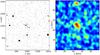 |
Fig. 1 Left: finding chart of an example artificial MASSCLEAN cluster embedded in a field of stars. Right: center determination via a two-dimensional KDE. |
2.2. Radius determination
A reliable radius determination is essential to the correct assignation of membership probabilities (Sánchez et al. 2010). There are several different definitions of SC radius in the literature, and we have chosen to assign the radius as the usually employed value where the radial density profile (RDP) stabilizes around the field density value. The RDP is the function that characterizes the variation of the density of stars per unit area with the distance from the cluster’s central coordinates. The field density is the density level in stars/area of combined background and foreground stars that gives the approximate number of contaminating field stars per unit of area that are expected to be spread throughout the observed frame, including the cluster region. Our “cluster radius” rcl, is thus equivalent to the “limiting radius” Rlim defined in Bonatto & Bica (2005) and Maia et al. (2014), the “corona radius” r2 defined in Kharchenko et al. (2005b) and the “radial density profile radius”, RRDP, used in Bonatto & Bica (2009), Pavani et al. (2011), and Alves et al. (2012).
2.2.1. Radial density profile
The RDP is usually obtained generating concentric circular rings of increasing radius values around the assigned cluster center, counting the number of stars that fall within each ring and dividing it by its area. The strategy we developed is similar but uses concentric square rings instead of circular rings, generated via an underlying 2D histogram/grid in the positional space of the observed frame. The bin width of this positional histogram is obtained as 1% of whichever spatial dimension spans the smallest range in the observed frame (i.e., min(Δx, Δy)/100). This (heuristic) value is small enough to provide a reasonable amount of detail, but not too large as to hide important features in the spatial distribution (e.g., a sudden drop in density)8.
The first RDP point is calculated by counting the number of stars in the central cell (or bin) of the grid, which is considered the first square ring, with a radius of half the bin width, divided by the area of the cell. Following that, we move to the eight adjacent cells (up, down, left, right: i.e., the second square ring with a radius of 1.5 bin widths), and repeat the calculus to obtain the second RDP point by dividing the stars in those eight cells by their combined area. The process is repeated for the next 16 cells (third square ring, radius of 2.5 bin widths), then the next 24 (fourth square ring, radius of 3.5 bin widths) and so forth, stopping when ~75% of the length of the frame is reached. This algorithm has the advantage of working with clusters located near a frame’s edge or corner with no complicated algebra needed to estimate the area of a severed circular ring, since cells/bins that fall outside the frame’s boundaries are easily recognized and thus not accounted for in the calculation of the RDP point’s total area. Eventually, the RDP function could be extended to accept a bad pixel mask to correctly avoid empty regions in frames either vignetted or with complicated geometries, or even zones with bad photometry.
2.2.2. Field density
The field density value is used by the radius finding function as the stable condition where the RDP reaches the level of the assumed homogeneous field star contamination present. This last requirement is important, and observed frames with a highly variable field star density should be treated with caution, eventually providing a manual estimation for the cluster radius.
The field density is usually obtained by manually selecting one or more field regions nearby, but not overlapping, that of the cluster, and calculating the number of stars divided by the total area of the region(s). This approach requires either an initial estimate of the cluster’s size or a large enough observed frame, such that the field region(s) can be selected far enough from the cluster’s center to avoid including possible members in the count. We developed a simple method for the determination of this parameter that allows us to fully automatize its estimation, no matter the shape or extension of the observed frame, using the RDP points through an iterative process. It begins with the complete set of points and obtains its median and standard deviation (1σ) values, to then reject the point located the farthest outside the 1σ range around the median. This step is repeated, with one RDP point less each time in the set, until no points are left outside the 1σ level. The final mean density value will have converged to the expected field density.
2.2.3. Cluster radius
The cluster’s radius defined above, rcl, is obtained combining the information from the RDP and the field star density, dfield. The algorithm searches the RDP for the point where it “stabilizes” around the dfield value, using several tolerance thresholds to define when the “stable” condition is met. This technique has proven to be very robust, assigning reasonable radius estimates even for scarcely populated or highly contaminated SCs without the need for user intervention at any part of the process.
2.2.4. King profile
Fitting a three-parameter (3P) King’s profile (King 1962) is not always possible because of low star counts in the cluster region and high field star contamination (Janes 2001). A two-parameter (2P) function where the tidal radius rtidal is left out and only the maximum central density and core radius rcore are fitted, is much easier to obtain. Some authors have recurred to somewhat elaborated schemes to achieve convergence of the fitting process with all three parameters (Piskunov et al. 2007). Our approach is to first attempt a 3P fit to the RDP and, if that is not possible because of either no convergence or an unrealistic rtidal, fall back to a 2P fit. The 3P fit is discarded if the tidal radius converges to a value greater than 100 times the core radius, which would imply a concentration parameter c> 2 comparable to that of globular clusters (Hillenbrand & Hartmann 1998). The formulas for the 3P and 2P functions are standard, presented for example in Alves et al. (2012).
Figure 2 shows as black dots (each one with its poissonian error bar) the RDP points obtained for a cluster manually generated with a tidal radius of rtidal = 250 px. The field density value, the 2P King fit with the obtained core radius rcore and the value for rcl along with its uncertainty are also shown.
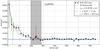 |
Fig. 2 Radial density profile of cluster region. Black dots are the stars /px2 RDP points taking the cluster center as the origin; the horizontal blue line is the field density value dfield, as indicated in Sect. 2.2.2; the red arrow marks the assigned radius with the uncertainty region marked as a gray shaded area; a 2P King profile fit is indicated with the green broken curve with the rcore (core radius) value shows as a vertical green line. |
2.3. Members and contamination estimation
2.3.1. Members estimation
We estimate the total number of probable cluster members following two approaches. The first is based on the 3P King profile fitting and utilizes the integral of the RDP from zero to rtidal above the estimated star field density (see Eq. (3) in Froebrich et al. 2007). This method will only work if the 3P fit converged and if it did so to a reasonable tidal radius, otherwise the result can be quite overestimated. The second approach is based on a simple star count: multiplying dfield by the cluster’s area Acl (given by the rcl radius), we get nfl, which is the approximate number of field stars inside the cluster region. The final estimated number of cluster members, ncl, is obtained subtracting this value to the actual number of stars within the rcl boundary ncl + fl: 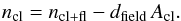 (1)Both methods give the approximate number of members down to the faintest magnitude observed, which means that they are dependent on the completeness level.
2.3.2. Contamination index
The contamination index parameter (CI) is a measure of the field star contamination present in the region of the SC. It is obtained as the ratio of field stars density dfield defined previously, over the density of stars in the cluster region. This last value is calculated as the ratio of the number of stars in the cluster region ncl + fl, counting both field stars and probable members, to the cluster’s total area Acl: 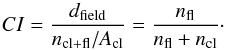 (2)A CI close to zero points to a low field star contamination affecting the cluster (ncl ≫ nfl). If the CI takes a value of 0.5, it means that an equal number of field stars and cluster members are expected in the cluster region (ncl ≃ nfl), while a larger value means that there are on average more field stars than cluster members expected within the limit defined by rcl (ncl<nfl). A large CI does not necessarily imply a high density of field stars in general, but when compared to the density of cluster members in the cluster region. As we will see in Sect. 3, this parameter proves to be a very reasonable estimator for the internal accuracy associated with the cluster parameters derived by ASteCA.
2.4. Error based rejection
Measured stars have photometric errors that tend to increase as they move toward fainter magnitudes. It is necessary to perform a filtering prior to the cluster analysis so that only stars with error values reasonably small are taken into consideration and artifacts left over from the photometry process are removed. To this end, ASteCA includes three routines to reject stars/objects with photometric errors beyond a certain limit; the results of each can be seen in Fig. 3 for a V vs. (B − V) CMD, which we will be using in all the example images that follow in this section.
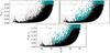 |
Fig. 3 Top: maximum error rejection method (left) and exponential curve method (right). Bottom: “eye fit” method. Rejected stars are shown as green crosses, and the horizontal dashed red line is the maximum error value accepted. See text for details. |
The first routine in the figure (top left) is a simple maximum error based algorithm that rejects any star beyond a given limit. A second method (top right) incorporates an exponential function to limit the region of accepted stars. The third method (bottom), referred as “eye fit” since it attempts to imitate how one would trace an upper error envelope by eye, is similar to the previous method, but uses a combination of an exponential function and a third degree polynomial to separate accepted and rejected stars. Notice that stars with errors beyond the limits in either magnitude or color will be rejected. This explains why in the bottom diagram of Fig. 3 some rejected stars can be seen lying below the curve for the (B − V) color: it means these stars had photometric errors above the curve in the V magnitude error diagram (not shown). As can be seen in Fig. 3, brighter stars can be treated separately to prevent the method from rejecting early type stars with error values above the average for the brightest region. Alternatively no rejection method can be selected, in which case all stars are considered by the code. The parameters of these methods can be adjusted via the input data file used by ASteCA. We do not take those stars rejected by this function into account in any of the processes that follow.
2.5. Cluster and field stars regions
ASteCA delimitates several field regions around the cluster region, each field region having the same area as that of the cluster. These field regions are used by those functions that require removing the contribution from field stars (see Sect. 2.6) and those that compare the cluster region’s CMD with CMDs generated from field stars (see Sects. 2.7 and 2.8). Each region is obtained in a spiral-like fashion to maximize the available space in the observed frame. The left diagram in Fig. 4 shows how this assignment is completed with stars belonging to the same field region plotted with the same color. The CMD of both the cluster region and the combined field regions is shown at right with their stars plotted in red and gray, respectively.
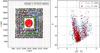 |
Fig. 4 Left: cluster region centered in the frame and 15 field regions of equal area defined around it. Adjacent field stars with the same color belong to the same field region (notice that only four colors are used and they start repeating themselves in a cycle). Right: CMD showing the cluster region stars as red points, stars in the combined surrounding field regions in gray, and rejected stars by the error rejection function as green crosses. |
2.6. Luminosity function and integrated color
The luminosity function (LF) of a SC gives the number of stars per magnitude interval and may be thought of as a projection of its CMD on the magnitude axis. This results in a simplified version of the CMD that allows for, in some cases, a quick estimation of certain features: for example, the main sequence turn off (TO). Integrated colors are often used as indicators of age, especially for very distant unresolved star clusters, and can also provide insights on a SC’s mass and metallicity (Fouesneau & Lançon 2010; Popescu et al. 2012). ASteCA provides both the LF and the integrated color of the SC, cleaned from field stars contribution whenever possible, i.e., depending on the availability of field stars in the observed frame.
The LF curve for the cluster region with field stars contamination, averaged field regions scaled to the cluster’s area Acl, and resulting clean cluster region can be seen in the left panel of Fig. 5 in red, blue, and green, respectively. The clean region is obtained by subtracting the field regions LF from the cluster plus field regions LF bin by bin. The completeness magnitude limit is also provided, estimated as the value were the total star count begins to drop.
An integrated magnitude curve for each observed magnitude is obtained via the standard relation (Gray 1965): 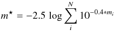 (3)where mi is the apparent magnitude of a single star and the sum is performed over all the N relevant stars, depending on the region being analyzed. Equation (3) is applied to both magnitudes that make up the cluster’s CMD (when available) in the cluster region contaminated by field stars and in the field regions defined around it, as seen in Sect. 2.5. The resulting curves are shown in the right diagram of Fig. 5 in red and blue, where the curves for the field regions (blue) are obtained interpolating among all the field regions to generate a single average estimate. The final integrated magnitude value is the minimum value attained by each curve after which Pogson’s relation is used to clean each cluster region magnitude from the field regions contribution. Combining both cleaned integrated magnitudes gives the cleaned cluster region integrated color, as shown in the diagram mentioned above.
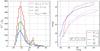 |
Fig. 5 Left: LF curves for the cluster region plus field star contamination (red), averaged field regions scaled to the cluster’s area (blue), and clean cluster region (green); completeness limit shown as a dashed black line. Right: integrated magnitudes versus magnitude values for the cluster region (plus field star contamination) in red and average field regions in blue. |
2.7. Real cluster probability
Assigning a probability to a detected spatial overdensity of being a true stellar cluster rather than a random field stars overdensity, is particularly useful in the study of open cluster remnants (Pavani & Bica 2007), and, in general, for OCs poorly populated and not easily distinguishable from their surroundings. This probability can be evaluated with the kde.test statistical function provided by the ks package9 (Duong 2007). The function applies a two-dimensional kernel density estimator (KDE) based algorithm, able to broadly asses the similarity between the arrangement of stars in two different CMDs (i.e., a two-dimensional photometric space), where the result is quantified by a p-value10. A strict mathematical derivation of the method can be found in Duong et al. (2012). The null hypothesis, H0, is that both CMDs were drawn from the same underlying distribution, with a lower p-value indicative of a lower probability that H0 is true. This function is applied to the cluster region’s CMD compared with every defined field region’s CMD, which results in a set of “cluster vs. field region” p-values. Each field region is also compared with the remaining field regions, thus generating a second set now of “field vs. field region” p-values, representing the behavior of those CMDs we expect to have a similar arrangement. The entire process is repeated a maximum of 100 times, in each case applying a random shift in the position of stars in the CMDs to account for photometric errors. The final sets of p-values are smoothed by a one-dimensional KDE to obtain the curves shown in Fig. 6. The blue curve (KDEcl) represents the cluster vs. field region CMD analysis, while the red curve (KDEfl) is the field vs. field region curve. For a true cluster, we would expect the blue curve to show lower p-values than the red curve, meaning that the cluster region CMD has a quite distinctive arrangement of stars when compared to surrounding field regions CMDs. Since both curves represent probability density functions, their total area is unity; furthermore, their domains are restricted between [0, 1] (a small drift beyond these limits is due to the 1D KDE processing). This means that the total area that these two curves overlap (shown in gray in the figure) is a good estimate of their similarity and thus proportional to the probability that the cluster region holds a true cluster. An overlap area of 1 implies that the curves are exactly equal, which points to a very low probability of the overdensity being a true cluster and the opposite is true for lower overlap values. We then assign the probability of the overdensity being a real cluster as 1 minus the overlap between the curves and call it  . In the left panel of Fig. 6, we show the analysis applied to a true synthetic cluster and, as expected, the KDEcl curve shows much lower values than the KDEfl curve, with a final value of close to 1. At right, a field region where no cluster is present is analyzed; this time the curves are almost identical and the obtained probability very low.
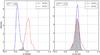 |
Fig. 6 Left: function applied on a synthetic cluster. The curves are clearly separated with the blue curve (cluster vs. field regions CMD analysis) showing much lower values; the final probability value obtained is close to 1 (or 100%). Right: same analysis performed on a random field region; the curves are now quite similar, resulting in a very low probability of the region containing a true stellar cluster. |
2.8. Field star contamination
The task of disentangling cluster members from contaminating foreground and background field stars is an important issue, particularly when SCs are projected toward crowded fields and/or with an apparent variable stellar density (Krone-Martins & Moitinho 2014, hereafter KMM14). Most observed SCs suffer from field star contamination to some extent and only in those systems close and massive enough can this effect be dismissed while at the same time ensuring a reasonably accurate study of their properties.
Numerous decontamination algorithms (DA) can be found throughout the literature, all aimed at objectively grouping observed stars into one of two classes: field stars or true cluster members. One of the simplest approaches consists of removing stars placed within a given limiting distance from the cluster’s Main Sequence (MS), defined by an arbitrary process (Claria & Lapasset 1986; Tadross 2001; An et al. 2007; Roberts et al. 2010). Proper motions (PM) are known to be a good discriminant between these classes. Techniques making use of PMs go back to the Vasilevskis-Sanders (V-S) method (Vasilevskis et al. 1958; Sanders 1971), which modeled cluster and field stars as a bi-variate Gaussian distributions in the vector point diagram (VPD) solving iteratively the resulting likelihood equation. The original method has been largely improved since and is present in numerous works (Stetson 1980; Zhao & He 1990; Kozhurina-Platais et al. 1995; Wu et al. 2002; Balaguer-Nunez et al. 2004; Javakhishvili et al. 2006; Frinchaboy & Majewski 2008; Krone-Martins et al. 2010; Sarro et al. 2014).
Although PM-based methods tend to be more accurate in determining membership probabilities (MP), the requirement of precise PMs, usually only available for relatively bright stars (KMM14), severely restricts their applicability. Photometric multiband data is abundant, on the other hand, as it is much easier to obtain, which is why many photometric-based star field DAs have long been proposed. Ozsvath (1960) developed one of the earliest by assigning MPs to stars located inside the cluster region according to the difference in stellar-density found in adjacent field regions of comparable size. Similar algorithms can be found applied with small variations in a great number of articles (Baade 1983; Mateo & Hodge 1986; Chiosi et al. 1989; Mighell et al. 1996; Bonatto & Bica 2007; Maia et al. 2010; Pavani et al. 2011; Bukowiecki et al. 2011, etc.). Some authors have attempted to refine this method by utilizing regions of variable sizes instead of boxes of fixed sizes, to compare the CMDs of field stars and stars within the cluster region (Froebrich et al. 2010; Piatti & Bica 2012). The recently developed UPMASK11 algorithm presented in KMM14 is a more sophisticated statistical technique for field star decontamination, which combines photometric and positional data and has the advantage of not requiring the presence of an observed reference field region to be able to assign membership probabilities.
We created our own Bayesian DA, described below, broadly based on the method detailed in Cabrera-Cano & Alfaro (1990) (nonparametric PMs-based scheme that follows an iterative procedure within a Bayesian framework).
2.8.1. Method
We begin by generating three regions from the observed frame: the cluster region C containing a mix of field stars and cluster members (i.e., those stars within the cluster radius rcl), a field region B containing only field stars (with the same area as that of the cluster), and a hypothetical clean cluster region A containing only true cluster members (which we do not have). We can interpret this through the relation A + B = C, meaning that a clean cluster region A plus a region of field stars B, results in the observed contaminated cluster region C. The membership problem can be reduced to this: if we take a random star from C, what is the probability that this star is a true cluster member (∈ A) or just a field star (∈ B)? In other words, we want to estimate its MP.
The hypotheses involved can therefore be expressed as:
-
H1: the star is a true cluster member (∈ A).
-
H2: the star is a field star (∈ B).
These hypotheses are exclusive and exhaustive, which means that either one of them must
be true; we are interested in particular in H1 to derive MPs for every star in the
cluster region. From
Bayes’ theorem12 we can obtain P(H1 |
D)j or the
probability, given the data D (i.e., the photometry for all stars), that
H1 is true for a given star
j picked
at random from the observed cluster region C; this probability is thus equivalent to the MP
of star j,
MPj.
The priors for H1 and H2 are
P(H1) =
(NA/NC)
and P(H2) =
(NB/NC)
, respectively, where NA, NB, and NC are the number of
stars in regions A, B, and C. Combining this with the likelihoods
LA,j =
P(D |
H1)j and
LB,j =
P(D |
H2)j for
star j, the
final form of the probability can be written as 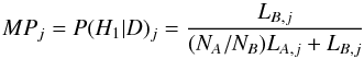 (5)where
the formula for the likelihood of star j is
(5)where
the formula for the likelihood of star j is ![\begin{eqnarray} L_{X,j} &= &\frac{1}{N_X} \sum_{i=1}^{N_X} \frac{1}{\sigma_m(i,j) \sigma_c(i,j)}\nonumber \\ &&\quad\times \exp\left[\frac{-(m_i - m_j)^2}{2 \sigma_m^2(i,j)}\right] \exp\left[\frac{-(c_i - c_j)^2}{2 \sigma_c^2(i,j)}\right] \label{eq:likel} \end{eqnarray}](/articles/aa/full_html/2015/04/aa24946-14/aa24946-14-eq66.png) (6)with
X ∈ { A,B
}. The parameters (m,c) are magnitude and color
and (σm,σc)
their respective photometric uncertainties of the form
(6)with
X ∈ { A,B
}. The parameters (m,c) are magnitude and color
and (σm,σc)
their respective photometric uncertainties of the form  (7)Ideally we will
have more than one field region defined surrounding the cluster region13 and we assume K such field regions:
{
B1,B2,B3,...BK
}. Each one of these K regions allows us to obtain a MP value for
every star j in C: MPi,j;
i = 1...K; j =
1...NC.
(7)Ideally we will
have more than one field region defined surrounding the cluster region13 and we assume K such field regions:
{
B1,B2,B3,...BK
}. Each one of these K regions allows us to obtain a MP value for
every star j in C: MPi,j;
i = 1...K; j =
1...NC.
The missing piece of information in this method so far is the clean cluster region
A. To
approximate it, we randomly remove NBi
(i = 1...K) stars from the
observed cluster region C, which results in a broad estimate of
A, under
the assumption that we are mainly removing field stars. This assumption does not hold
for heavily contaminated SCs and, as we will see in Sect. 3, leads to the DA behaving poorly for SCs with high CI values. To ensure that
the A
region is a fair statistical representation of a noncontaminated cluster region, the
entire process is iterated Q times14,
each time removing from C a new set of NBi
random stars. This means that for every j star in C a total of
K ∗
Q values for its MP are obtained, which can be
finally combined into a single probability taking the arithmetic mean
 (8)Figure 7 shows the result of applying the algorithm on an
example OC, see caption for details. The DA can accept an input file with membership
probabilities manually assigned to individual stars, this allows fixing high
probabilities to known members obtained via a secondary method (spectroscopy). The main
strength of the method resides in its ability to eventually include extra information,
such as other observed magnitudes, colors, radial velocities, or proper motions, by
simply extending Eq. (6) adding an extra
exponential term accounting for it.
(8)Figure 7 shows the result of applying the algorithm on an
example OC, see caption for details. The DA can accept an input file with membership
probabilities manually assigned to individual stars, this allows fixing high
probabilities to known members obtained via a secondary method (spectroscopy). The main
strength of the method resides in its ability to eventually include extra information,
such as other observed magnitudes, colors, radial velocities, or proper motions, by
simply extending Eq. (6) adding an extra
exponential term accounting for it.
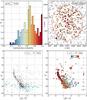 |
Fig. 7 Top: distribution of MPs (left), probmin is the value that separates the upper half of stars with the highest MPs from the lower half and spatial chart (right) with stars in the cluster region colored by their MPs. Bottom: CMD of the observed cluster region (left) with rejected stars marked as green crosses and the same CMD minus the rejected stars (right) with coloring according to each star’s MPs. |
2.9. Cluster parameters determination
The most common method for obtaining the parameters of an SC is still the simple by-eye isochrone match on a CMD, examples of this visual approach to estimate theoretical isochrone vs. observed cluster best fits are abundant (e.g., Bonatto & Bica 2009; Maia et al. 2010; Majaess et al. 2012; Kharchenko et al. 2013; Carraro et al. 2014, etc.). The drawbacks of this method include the obvious subjectivity involved in the matching process and the inability to attach an uncertainty to the values obtained, along with the unavoidable inefficiency when attempting to apply it to sets of several hundreds or even thousands of SCs, as done, for example, in Buckner & Froebrich (2014) where the authors manually fitted over 2300 isochrones on near-infrared CMDs.
A summary of methods that make use of certain geometrical evolutionary indicators (e.g., the δ magnitude and color indices, Phelps et al. 1994) can be seen in Hernandez & Valls-Gabaud (2008; HVG08), along with approaches to the estimation of star cluster parameters based on full CMD analysis. This same article introduces a statistical technique based on using the density of stars along an isochrone to lift the geometric age-metallicity degeneracy when attempting a match.
In the pioneering work of Romeo et al. (1989), the authors applied the standard technique of generating synthetic populations and comparing them with an observed simple stellar population CMD to study its properties. Since then, the “synthetic CMD method” has been widely used on simple stellar populations (Sandrelli et al. 1999; Carraro et al. 2002; Subramaniam et al. 2005; Singh Kalirai 2006; Kerber et al. 2007; Girardi et al. 2009; Cignoni et al. 2011; Donati et al. 2014, etc.). An expansion of the method can be found applied with little adjustments to the recovery of SFHs of nearby galaxies (Ferraro et al. 1989; Tosi et al. 1991; Tolstoy & Saha 1996; Hernandez et al. 1999; Dolphin 2002; Frayn & Gilmore 2002; Aparicio & Hidalgo 2009; Small et al. 2013)15.
Decontamination algorithm and cluster parameters estimation processes have been coupled in various recent works. This can be seen for example in the series of articles by Kerber et al. (Kerber et al. 2002; Kerber & Santiago 2005) where an estimate of the density of field stars in the cluster region is used to implement a field star removal process together with a cluster CMD modeling strategy that selects the best observed vs. artificial fit via a statistical tool; the white dwarf based Bayesian CMD inversion technique developed in von Hippel et al. (2006) expanded and coupled with a basic field star cleaning process in van Dyk et al. (2009); the synthetic cluster fitting method introduced in Monteiro et al. (2010; MDC10, further developed in the articles Dias et al. 2012; Oliveira et al. 2013), which includes a likelihood-based decontamination algorithm; the work by Pavani et al. (2011) where CMD density-based membership probabilities are given to stars within the cluster region to later apply a very basic isochrone fitting process that makes use of stars close to a given isochrone in CMD space; and the articles by Alves et al. (2012) and Dias et al. (2014), who employ the same membership probability assignment method used in Pavani et al. (2011) coupled with a slightly improved isochrone fitting algorithm based on the one developed by MDC10, but applied to a Hess diagram of the CMD instead of the full CMD. In Buckner & Froebrich (2013) the membership assignment method presented in Froebrich et al. (2010), a variation of the Bonatto & Bica (2007) algorithm, is used in conjunction with the Besançon model of the galaxy16 to derive distances to OCs, based on foreground stars density estimations.
In a series of papers by Kharchenko et al. where the COCD17 and MWSC18 catalogs are developed (respectively, Kharchenko et al. 2005a; Schmeja et al. 2014, and references therein), the authors develop a pipeline to analyze OCs with available PMs, capable of determining a handful of properties: center, radius, number of members, distance, extinction, and age. The method is neither entirely objective nor automatic since the user is still forced to manually intervene adjusting certain variables to generate reasonable estimates for the cluster parameters.
The general synthetic CMD method applied by ASteCA has been outlined previously in Tolstoy & Saha (1996) and Hernandez et al. (1999) in the context of star formation history recovery. We adopt the procedures adapted to single stellar populations described in HVG08 and MDC10 and broadly combine them to obtain the optimal set of cluster parameters associated with the observed SC. The theoretical isochrones employed are taken from the CMD v2.5 service19 (Girardi et al. 2000), but eventually any set of isochrones could be used with minimal changes needed to the code.
2.9.1. Method
Given a set A = { a1,a2,...,aN } of N observed stars in a cluster region, we want to find the model Bi out of a set of M models B = { B1,B2,...,BM } with the highest probability of resulting in the observed set A. This is P(Bi | A) or the probability of Bi given A. Each Bi model represents a theoretical isochrone of fixed metallicity (z) and age (a), moved by certain distance (d) and extinction values (e), meaning the models in B are fully determined as points in the 4-dimensional space of cluster parameters: Bi = Bi(z,a,d,e). Finding the highest P(Bi | A) can be reduced to maximizing the probability of obtaining A given Bi, P(A | Bi), i.e., the probability that the observed SC A arose from a Bi model20. The first step in determining P(A | Bi) is to define how the Bi models are generated. The well-known age-metallicity degeneracy is, as stated in HVG08 and Cerviño et al. (2011), geometrical in nature21, and the result of considering only the shapes of the isochrones when fitting an observed SC, instead of also taking the density of stars along them into account. There are two ways of accounting for the star density in a given isochrone: through a mass density parameter as done in HVG08 or, as done in MDC10, generating correctly populated Bi models as synthetic clusters; we have chosen to apply the latter.
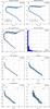 |
Fig. 8 Generation of a synthetic cluster starting from a theoretical isochrone of fixed parameters (metallicity, age, distance, and extinction) populated using the exponential IMF of Chabrier (2001). See text for a description of each panel. |
The process by which a synthetic cluster of given z, a, d, and e parameters, or Bi(z,a,d,e) model, is generated is shown in Fig. 8. Panel a shows a random theoretical isochrone picked with certain metallicity and age values, densely interpolated to contain 1000 points throughout its entire length; notice even the evolved parts are taken into account. In panel b the isochrone is shifted by some extinction and distance modulus values, emulating the effects these extrinsic parameters have over the isochrone in a CMD. At this stage the synthetic cluster can be objectively identified as a unique point in the 4-dimensional space of parameters. Panel c shows the maximum magnitude cut performed according to the maximum magnitude attained by the observed SC being analyzed. We see that the total number of synthetic stars drops. An initial mass function (IMF) is sampled as shown in panel d in the mass range [~0.01−100] M⊙ up to a total mass value Mtotal provided via the input data file, set to Mtotal = 5000 M⊙ by default22. Currently ASteCA lets the user choose between three IMFs (Kroupa et al. 1993; Chabrier 2001; Kroupa 2002), but there is no limit to the number of distinct IMFs that could be added. The distribution of masses is then used to obtain a correctly populated synthetic cluster, as shown in panel e, by keeping one star in the interpolated isochrone for each mass value in the distribution. The drop seen for the total number of stars is due to the limits imposed by the mass range of the post-magnitude cut isochrone. A random fraction of stars are assumed to be binaries, by default the value is set to 50% (typical for OCs, von Hippel 2005) with secondary masses drawn from a uniform distribution between the mass of the primary star and a fraction of it given by a mass ratio parameter set by default to 0.7; both figures can be modified in the input data file. Panel f shows the effect of binarity on the position of stars in the CMD. Each synthetic cluster is finally perturbed by a magnitude completeness removal function and an exponential error function, where the parameters for both are taken from fits done on the observed SC and are thus representative of it. Panels g and h show these two processes with the resulting Bi(z,a,d,e) synthetic cluster shown in the former.
With the B set of synthetic clusters generated, the next step is to maximize P(A | Bi) to find the best fit cluster parameters for the observed SC. The probability that an observed star aj from A is a star k from a given synthetic cluster Bi can be written as (HVG08) ![\begin{eqnarray} P(a_j|B_{i,k}) &=& \frac{1}{\sigma_m(j,k) \sigma_{\rm c}(j,k)}\nonumber \\ && \quad\times \exp\left[\frac{-(m_j - m_k)^2}{2 \sigma_m^2(j,k)}\right] \quad \exp\left[\frac{-(c_j - c_k)^2}{2 \sigma_c^2(j,k)}\right] , \end{eqnarray}](/articles/aa/full_html/2015/04/aa24946-14/aa24946-14-eq100.png) (9)where the same notation as that used in Eqs. (6) and (7) applies.
(9)where the same notation as that used in Eqs. (6) and (7) applies.
Summing over the Mi stars in Bi gives the probability that aj came from the distribution of stars in the synthetic cluster 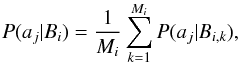 (10)where the 1 /Mi normalization factor prevents models with more stars having artificially higher probabilities. The final probability for the entire observed SC, A, to have arisen from the model Bi, also called likelihood, is obtained combining the probabilities for each observed star as
 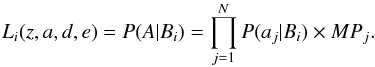 (11)Following MDC10, we include the MPs obtained by the DA for every star in the cluster region, MPj, as a weighting factor. The problem is then reduced to finding the Bi(z,a,d,e) model that produces the maximum Li value for a fixed A set or observed cluster region.
2.9.2. Genetic algorithm
Obtaining the best fit between A, the observed SC, and the set of M models/synthetic clusters B, is equivalent to searching for the maximum value in the 4-dimensional Li(z,a,d,e) surface and can be thought of as a global maximum/minimum optimization problem. The number M depends on the resolution defined by the user for the grid of cluster parameters; to calculate it we multiply the total number of values each parameter can attain (range divided by a step) for all the parameters, which is four in our case. For a not too dense grid, this number will become very high23, which makes the exhaustive search for the best solution in the entire parameter space not possible in a reasonable time frame.
Following HVG08, we have chosen to build a genetic algorithm (GA; see: Whitley 1994; Charbonneau 1995, for an in-depth description of the algorithm and references in HVG08) function into ASteCA to solve this problem. A GA is a method used to solve search and optimization problems based on a heuristic technique derived from the biological concept of natural evolution. We prefer it over similar approaches like the cross-entropy method described in MDC10 due mainly to its flexibility, which makes it easily adaptable to different optimization scenarios.
Instead of finding the best fit for A as the maximum likelihood value, we make the GA search for the minimum of its negative logarithm, which is a computationally more efficient variant![\begin{equation} \vec{L}_A(z^{\star}, a^{\star}, d^{\star}, e^{\star}) = {\rm min}\{-\log[L_i(z, a, d, e)] \,;\,i=1..M\} , \end{equation}](/articles/aa/full_html/2015/04/aa24946-14/aa24946-14-eq107.png) (12)where the ⋆ upper-script indicates the final best-fit cluster parameters assigned to the observed SC.
(12)where the ⋆ upper-script indicates the final best-fit cluster parameters assigned to the observed SC.
The implementation of the GA can be divided into the usual operators: initial random population, selection of models to reproduce, crossover, mutation, and evaluation of new models cycled a given number of “generations”. At the end of each generation the model that presents the best fit is selected and passed unchanged into the new generation to ensure that the GA always moves toward a better solution24.
Uncertainties for each parameter are obtained via a bootstrap process that runs the GA Nbtst times, each time resampling the stars in the observed SC with replacement (i.e., a given star can be selected more than once) to generate a new variation of the dataset A. After all these runs, the standard deviation of the values obtained for each parameter is assigned as the uncertainty for that parameter. Ideally the bootstrap process would require N [ ln(N) ] 2 runs to sample the entire bootstrap distribution (Feigelson & Babu 2012), where N is the number of stars within the cluster region. This is unfortunately not feasible even for a small OC25, so we settle for setting Nbtst = 10 by default, which the user can modify at will.
An example of the results returned by the GA is shown in Fig. 9. The top row shows the evolution of the minimal likelihood (Lmin ≡ LA) as generations are iterated with a black line, where it can be seen how the GA zooms in the optimal solution early on in the process; the method is known to be a very aggressive optimizer. The blue line is the mean of the likelihoods for all the chromosomes/models in a generation where each spike marked with a green dotted line denotes an application of the extinction/immigration operator. The middle row shows a density map of the solutions/models explored by the GA separated in two 2-dimensional spaces for visibility: at left, metallicity and age (intrinsic parameters) are shown and, at right, distance modulus and extinction (extrinsic parameters). The position of the optimal solution is marked as a dot in each plot, with the ellipses showing the uncertainties associated with the solution. The bottom row shows, at left, the CMD of the observed cluster region (A) colored according to the MPs obtained with the DA, and, at right, the best-fit synthetic cluster found. The isochrone from which the synthetic cluster originated is drawn in both panels.
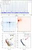 |
Fig. 9 Results of the GA applied over an example OC. See text for more details. |
2.9.3. Brute force
A brute force algorithm (BFA) function is also provided in case the parameter space can be defined small enough to allow searching throughout the entire grid of values. Unlike the GA, which has no clear stopping point, the BFA is always guaranteed to return the best global solution, after all the points in the grid have been analyzed. The BFA therefore does not need to apply a bootstrap process to assign uncertainties to the obtained cluster parameters, instead its accuracy depends only on the resolution of the grid. If the required precision in the final estimation of the cluster parameters is sufficiently small, the BFA can be preferable to the GA.
3. Validation of ASteCA
To validate ASteCA, we used a sample of 432 synthetic open clusters (SOCs) generated with the MASSCLEAN package26. Table 1 lists the grid of parameters taken into account. Each distance was assigned a fixed visual absorption value to cover a wide range of extinction scenarios; all distances are from the Sun.
MASSCLEAN parameters used for the generation of 432 SOCs.
We built V vs. (B − V) CMDs and spatial stellar distributions for each SOC with a limiting magnitude of V = 22 mag. The SOCs were generated with a tidal radius rtidal = 250 px and placed at the center of a star field region 2048 × 2048 px wide. Since MASSCLEAN returns SOCs with no photometric errors, the stars were randomly shifted according to the following error distribution: 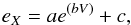 (13)where X stands for either the V magnitude or the (B − V) color, and the parameters a,b,c are fixed to the values 2 × 10⁻⁵, 0.4, 0.015, respectively. We also randomly removed stars beyond V = 19.5 mag to mimic incompleteness effects, using the expression
 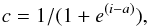 (14)where c represents the percentage of stars left after the removal process in the V magnitude bin i, and a is a random value in the range [ 2,4).
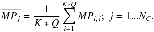
Figure 10 depicts an example for a 600 M⊙ SOC. The upper panels show the initial spatial stellar distribution (left) and CMD (right), respectively; the middle panels illustrate the behavior of the error distribution and incompleteness functions, while the bottom panels show the resulting cluster star field and the respective CMD. Likewise, Fig. 11 shows eight examples of SOCs generated with different masses and field-star contamination.
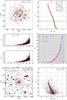 |
Fig. 10 Top: spatial distribution (left) of a SOC according to the parameters labeled in the respective CMD (right), wherein the green line indicates the magnitude limit adopted in the validation. Red symbols refer to cluster stars. Middle: photometric errors (left) and the completeness function (right) adopted. Bottom: resulting cluster star spatial distribution (left) with a circle representing the tidal radius and the corresponding CMD (right). |
Ranges used by the GA algorithm when analyzing MASSCLEAN SOCs.
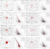 |
Fig. 11 Examples of SOCs produced as described in Sect. 3 with fixed metallicity and age, and varying total mass, distance, and visual absorption values. Symbols as in Fig. 10 (bottom panels). |
3.1. ASteCA test with synthetic clusters
We applied ASteCA for the 432 SOCs in automatic mode, which means that no initial values were given to the code with the exception of the ranges where the GA should look for the optimal cluster parameters, shown in Table 2. The relations connecting V, (B − V), visual absorption, and distance are of the form 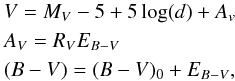 (15)where MV, (B − V)0 are the absolute magnitude and intrinsic color taken from the theoretical isochrone, d is the distance in parsecs, AV is the visual absorption, and the extinction parameter is fixed to RV = 3.1. In its current version, MASSCLEAN uses the Marigo et al. (2008) and Girardi et al. (2010) Padova isochrones, which adopt a solar metallicity of z⊙ = 0.019.
The results obtained by ASteCA are combined with the true values used to generate the SOCs in the sense true value minus ASteCA value:  (16)for the radius and the four cluster parameters, and the resulting deltas compared against the CI (defined in Sect. 2.3.2) assigned to the SOCs. We choose to use the CI not only because it is simple to obtain and useful to asses the field star contamination, but also because it can be easily calculated even for observed clusters, i.e., there is no requirement to know in advanced the true members of a cluster and the field stars within its defined region to obtain its CI. This independence from a priori unknown factors, in contrast for example with the similar contamination rate parameter defined in KMM14, means we can use the CI to extrapolate, with caution, the limitations and strengths of ASteCA gathered using SOCs, to observed OCs. In some of the plots below the natural logarithm of the CI is used instead to provide a clearer graphical representation of the results.
The SOCs generated via the MASSCLEAN package act as substitutes for observed OCs whose parameter values are fully known, and must not be confused with the synthetic clusters generated internally by ASteCA as part of the best model fitting method (Sect. 2.9.1). In what follows the former will always be referred to as SOCs and the latter either as “synthetic clusters” or “models”.
3.1.1. Structure parameters
As a first step, we analyze the center and radius determination functions, which are based on spatial information exclusively. To generate the final SOCs, the original MASSCLEAN clusters have a portion of their stars removed via the maximum magnitude cutoff and incompleteness functions, as shown in Fig. 10. The original center and radius values used to create them will clearly be affected by both processes, so an intrinsic scatter around these true values is expected independent from the behavior of ASteCA.
Figure 12 shows, at left, the distribution of the distances to the true center (1024,1024) px of the central coordinates found by the code (xo,yo) px as  (17)for all SOCs located closer than 90 px away from the true center, that is almost 90% (386) out of the 432 SOCs processed. The remaining 46 SOCs that were given center values farther away have on average less than 15 members and CI values larger than 0.7, thus the difficulty in finding their true center. Almost half of the sample was positioned less than 20 px away from the true center (shaded region in the figure), which represents 1% of the frame’s dimension in either coordinate.
In the right panel of Fig. 12, the delta difference for the radius is shown, as defined in Eq. (16), only for the subsample of 386 SOCs whose central coordinates were positioned closer than 90 px from the true center. In this case 50% of the subsample presented rcl radius values less than 19 px away from the true value used to generate the SOCs (rtidal = 250 px), with 90% of the subsample found to have values less than 57 px away. Considering the frame has an area of 2048 × 2048 px, these results are quite good.
As stated in Sect. 2.2, fitting a three-parameters King profile is not always possible, especially for clusters that show a low density contrast with their surrounding fields. About 76% of the above mentioned subsample of SOCs could have their 3P King profile calculated of which only two converged to values rtidal< 300 px with approximately ~80% returning values rtidal> 400 px. This overestimation of the tidal radius is due to the high dependence of the fitting process with the shape of the RDP, particularly for SOCs with low members counts. Internal tests showed that modifying the bin width of the 2D histogram used to obtain the RDP (see Sect. 2.2) by even 1 px can cause the 3P King profile to converge to a significantly different rtidal value. Care should be exercised thus when utilizing or interpreting the structure of an OC based on this parameter.
A clear correlation can be seen in Fig. 12 where the dispersion in both distance to the true center and departure from the true cluster radius increase for larger CI values.
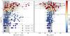 |
Fig. 12 Left: logarithm of the CI vs. difference in center assigned by ASteCA with true center. Sizes vary according to the initial masses (larger mean larger initial mass) and colors according to the distance (see colorbar to the right). Right: logarithm of the CI vs. radius difference (ASteCA minus true value) for each SOC. In both plots shaded regions mark the range where 50% of all SOCs are positioned and estimated errors are shown as gray lines. |
3.1.2. Probabilities and members count
The probability of being a real star cluster rather than an artificial grouping of field stars is assessed by the function described in Sect. 2.7. For each SOC whose central coordinates were found within a 90 px radius of the true central coordinates (90% of the SOCs, as stated in Sect. 3.1.1) their probability value can be seen in the left panel of Fig. 13 as filled circles. Diamonds represent those 46 instances were the center was detected far away from its true position meaning the comparison made to obtain the p-values, from which the probability is derived, was done mostly (and sometimes entirely) by contrasting a field region with other field regions. Expectedly, the probabilities found in these cases are very low having an average value of ~0.2. A few low mass distant SOCs with an average number of members of 33 can also be found in this region of low probability. This is unavoidable since high field stars contamination means that effectively separating true star clustering from random overdensities is not a simple task, especially for those systems with a very low number of members. Nevertheless, the large majority of SOCs are assigned high probability values, which points to the function being reliable even for clusters with high CIs and relatively few true members. In what follows these 46 “clusters” that were positioned far away from the true center, and are thus almost entirely composed of field stars, are dropped from the analysis.
In the right panel of Fig. 13 the relative error for the number of members is shown following the relation:  (18)where mntrue and mnasteca are the true number of members and the number of members calculated by ASteCA. Half of the SOCs had their number of members estimated within a 3% relative error (shaded region) and over 80% of them within a 20% relative error. The error can be clearly seen to increase primarily with the CI, but also with age given that older SOCs usually have fewer true members making them more susceptible to field star contamination.
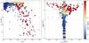 |
Fig. 13 Left: distribution of real cluster probabilities vs. CI. Sizes vary according to the initial masses (bigger size means larger initial mass) and colors according to the distance (see colorbar to the right). Circles represent values for SOCs and diamonds values obtained for field regions. Right: logarithm of the CI vs. relative error for the true number of members and that predicted by ASteCA for each SOC. Point markers are associated with ages as shown in the legend. The shaded region marks the range where 50% of all SOCs are positioned. |
3.1.3. Decontamination algorithm
To study the effectiveness of the decontamination algorithm (DA) described in Sect. 2.8, in assigning membership probabilities (MP) to true cluster members, we define two member index (MI) relations as: 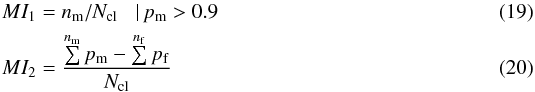 where nm and nf are the number of true cluster members and of field stars bound to be present within the cluster region (i.e., inside the boundary defined by the cluster radius), pm and pf are the MPs assigned to each of them by the DA, and Ncl is the total number of true cluster members. The index in Eq. (19), MI1, can be thought of as an equivalent to the true positive rate (TPR) defined in KMM14 as “the ratio between the number of real cluster members in the high probability subset and its total size”, where the high probability subset contains only true members with assigned probabilities over 90% (TPR90). The maximum value for this index is 1, attained when all true members are recovered with MP> 90%. The index MI2 defined in Eq. (20) rewards high probabilities given to true members but also punishes high probabilities given to field stars. The optimal value is 1, achieved when all true cluster members are identified as such with MP values of 1, and no field star is assigned a probability higher than 0. The index MI2 dips below zero when the added probabilities of field stars is larger than that of true members. In this case the DA can be said to have “failed” since it assigned a greater combined MP to nonmember (field) stars than to true cluster members.
To provide some context for the results, we compare both MIs obtained by the DA for each SOC with those returned by an algorithm of random probabilities assignation. The latter randomly assigns MPs uniformly distributed between [ 0,1 ] to all stars within the cluster region of a SOC. As can be seen in Fig. 14, the DA behaves very well up to a CI value of 0.4, where it shows a value of  (that is: an average ~78% of true members being recovered with MPs higher than 90%) and
  , which means field stars do not play an important role thus far. Between the range CI = (0.4,0.6) the MIs obtained for the DA begin looking increasingly similar to those obtained for the random probability assignation algorithm. This is noticeable especially for MI2 where the increased presence of field stars starts having a larger influence in its value. Beyond a CI of approximately 0.6 the DA breaks down as it apparently no longer represents an improvement over assigning MPs randomly.
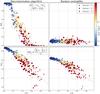 |
Fig. 14 Top left: member index defined in Eq. (19) vs. contamination index. Top right: same MI vs. CI plot except using the membership probabilities given by the random assignment algorithm. Bottom left: member index defined in Eq. (20) vs. contamination index. Bottom right: same MI vs. CI plot except using the membership probabilities given by the random assignment algorithm. Linear fits in each plot shown as dashed black lines. Sizes, shapes, and colors as in Fig. 12. |
3.1.4. Cluster parameters
The results for all cluster parameters are presented here for the entire set of SOCs, with the exception of those low-mass and highly contaminated systems that were rejected because the center finding function assigned their position far away from the real cluster center and are thus mainly a grouping of field stars (46 as stated in Sect. 3.1.1).
At this point it is important to remember that the accuracy of the results obtained for the cluster parameters depends not only on the correct working of the methods written within the code, but also on the intrinsic limitations of the photometric system selected and the type and number of filters chosen (see Anders et al. 2004; and de Grijs et al. 2005, for a discussion applied to the recovery of cluster parameters based on fitting observed spectral energy distributions). In our case, as stated at the beginning of Sect. 3, we opted to generate the SOCs for the validation process using only the VB bands of the Johnson system provided by MASSCLEAN to construct simple V vs. (B − V) CMDs. This not only means we are relying on a very reduced space of “observed” data (two-dimensional), but also that the resolution power of the analysis is necessarily limited by our selection of filters. The presence of a third band, particularly one below or encompassing the Balmer jump, would provide a CMD packed with more photometric information and quite possibly help reduce uncertainties in general. The U and B filters of the Johnson system for example can be combined to generate the (U − B) index, known to be sensitive to metal abundance, while bands located toward the infrared part of the spectrum are less affected by interstellar extinction. It is also worth stressing that the isochrone matching method is an inherently stochastic process. Even if the SOCs were generated without errors and incompleteness perturbations as isochrones populated via a given IMF, the randomness involved in producing the synthetic clusters used to match the best model, as explained in Sect. 2.9.1, would introduce an inevitable degree of inaccuracy in the final cluster parameters.
The plots in Fig. 15 show the dependence of the differences between the true value used to generate the SOCs and those estimated by ASteCA (Δparam) with the CI, for the four cluster parameters. The dispersion in the delta values tends to increase with the CI as do the errors with which these parameters are estimated by the code (horizontal lines).
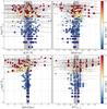 |
Fig. 15 Top left: metallicity differences in the sense true value minus ASteCA estimate vs. log (CI) with errors assigned by the code as gray horizontal lines. Top right: idem for log (age). Bottom left: idem for distance in kpc. Bottom right: idem for EB − V extinction. Shaded regions mark the ranges where 50% of all SOCs are positioned. Sizes, shapes, and colors as in Fig. 12. |
The metallicity is converted from z to the more usual [ Fe/H ] applying the standard relation [ Fe/H ] = log (z/z⊙) where z⊙ = 0.019, and contains about 25% of the sample below the largely acceptable error limit of ± 0.1 dex with 50% showing errors under ~0.28 dex (shaded region in top left plot of Fig. 15). There are no noticeable biases in the metallicities assigned by ASteCA, although the dispersion increases rapidly even for SOCs with low CI values.
The top right plot in Fig. 15 shows half of the sample located within ± 0.2 of their true log (age) values (shaded region). Many young SOCs with low CIs are assigned higher ages by ASteCA than those they were created with. This effect arises from the difficulty in determining the location of the TO point for those young clusters that have no evolved stars in their sequences. An example is shown in Fig. 16 for a SOC of log (age) = 7.0 where the age is recovered with a substantial error (0.9) even though the isochrone displays a very good fit.
Taking the subset of 132 analyzed young SOCs with log (age) = 7, we find that only 17% of them (23) had assigned ages that differ more than Δlog (age) > 1 with their true age values. This is the result of bad isochrone assignations, owing primarily to the combination of high field star contamination (CI ≃ 0.5, on average) and low total masses (~260 M⊙, on average) of these clusters. The remaining 83% of young clusters presented on average Δlog (age) ≃ 0.36, distributed as follows: almost half (62) were given ages deviating less than log (age) ≃ 0.3 from their true values, a third (43) showed Δlog (age) ≤ 0.2 and a fourth (33) presented Δlog (age) ≤ 0.1, or less than 26% relative error for the age expressed in years, which is quite reasonable. These results contrast with those obtained for the 254 analyzed older clusters (log (age) = [ 8,9 ]), which show that 80% of them have their true age values recovered within Δlog (age) ≤ 0.3, with an average deviation of Δlog (age) ≃ 0.16.
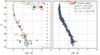 |
Fig. 16 Left: CMD of cluster region for a MASSCLEAN young SOC with MPs for each star shown according to the color bar at the top and the best-fit isochrone found shown in green. True age value is log (age) = 7.0. Right: best-fit synthetic cluster found along with the theoretical isochrone used to generate it in red. Cluster parameters and uncertainties shown in the top right box. |
Both the distance and extinction parameters, Fig. 15 bottom row, are recovered with a much higher accuracy, especially for SOCs with lower CI values. In the case of the distance half the sample is within a ± 0.2 kpc range from the true values (shaded region) and ~77% of the sample within ± 1 kpc. The dispersion in the EB − V color excess positions half of the sample below ± 0.04 mag (shaded region) and almost 90% below ~0.2 mag. There seems to be a correlation in the portion of SOCs with high CI, where clusters appear to be located simultaneously at larger distances and with lower extinction than their true values. Upon closer inspection we see that this is not the case, as shown by the positive correlation coefficient found between these two parameters.
The full correlation matrix (covariance matrix normalized by the standard deviations) for the deltas of all cluster parameters can be seen in Table 3.
Correlation matrix for the deltas defined for each cluster parameter.
The departures from the true distance and color excess values (Δdist and ΔEB − V) have no negative correlation but in fact a small positive correlation (0.4), meaning that as one increases so does the other. It is worth noting the small negative correlation value found between metallicity and age, which points at a successful lifting of the age-metallicity degeneracy problem by the method. The well-known age-extinction degeneracy, whereby a young cluster affected by substantial reddening can be fitted by an old isochrone with a small amount of reddening, stands out as the highest correlation value (HVG08, de Meulenaer et al. 2013). The positive correlation between metallicity values and the distance has also been previously mentioned in the literature (e.g., Hasegawa et al. 2008).
3.1.5. Limitations and caveats
An important source responsible for inaccuracies when recovering the SOCs cluster parameters, mainly for those in the high CI range, comes as a consequence of the way the theoretical isochrones are employed in the synthetic cluster fitting process. In HVG08 the authors limit the isochrones to below the helium flash to avoid issues with nonlinear variations in certain regions of the CMD. Unlike this work, we chose to avoid ad hoc cuts in the set of theoretical isochrones and instead use their entire lengths to generate the synthetic clusters, which means using also their evolved parts. Figure 17 shows how this affects the way synthetic clusters are fitted to obtain the optimal cluster parameters, for a SOC of log (age) = 9 located at 5 kpc with a color excess of EB − V ≃ 0.97 mag.
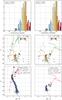 |
Fig. 17 Left column: top, MPs distribution for an old SOC where the cut is done for a value of probmin = 0.75; center, CMD of cluster region with MPs for each star shown according to the color bar at the top and the best-fit isochrone found shown in green; bottom, best-fit synthetic cluster found along with the theoretical isochrone used to generate it in red, cluster parameters and uncertainties shown in the top right box. Right column: top, idem above with probability cut now done at probmin = 0.85; center, idem above with new best-fit isochrone; bottom, idem above showing new synthetic cluster and improved cluster parameters. |
The left column of the figure shows at the top the distribution of MPs found by the decontamination algorithm with the probability cut used by the GA made at probmin = 0.75. In the middle left portion the CMD of the cluster region is shown along with the best matched theoretical isochrone found using this MP minimum value and the synthetic cluster generated from it at the bottom. As can be seen the highly evolved parts of the isochrone are being populated, which means these few stars will also be matched with those from the SOC with MPs above the mentioned limit, thus forcing the match toward very unreliable cluster parameters. In such a case, a simple solution is to increase the minimum MP value used by the genetic algorithm to obtain the best observed-synthetic cluster fit, as shown in the right column of Fig. 17. Here we were able to change the unreliable cluster parameters obtained for the SOC using a minimum MP value of probmin = 0.75, to a very good fit with small errors by simply increasing said value to probmin = 0.85. This slight adjustment restricts the SOC stars used in the fitting process to those in the top 15% MP range, which translates to a much more reasonable isochrone matching and improved cluster parameters as seen in the middle and bottom plots of the right column. Were this process to be replicated in the full SOCs sample, we would surely see an overall improvement in the determination of the cluster parameters.
Number of poorly populated (Nmemb ≤ 50) SOCs that had their parameters recovered with relative errors (er) below the given thresholds; percentage of total sample (82) is shown in parenthesis.
Clusters with a scarce number of stars and high field star contamination are particularly difficult to analyze for obvious reasons. The subset of our sample of SOCs containing the most poorly populated clusters coincides with the highest contaminated SOCs analyzed: 82 clusters averaging less than 50 true members each with CI> 0.5 (i.e., more field stars than true members within the cluster region). Table 4 shows the relative errors (defined as [True value – ASteCA value]/True value) obtained in this subset for each parameter. While distance and extinction display the best match with the true values, we see that the age is the most affected parameter when analyzing clusters with very few members. Still, we find that over half of this subset shows absolute age errors below log (age) = 0.3, which is largely acceptable. The 40 clusters with the largest age relative errors (er> 90%) show no definitive tendency toward any particular age, being distributed as 16, 15, and 9 clusters for log (age) values of 7, 8, and 9, respectively.
Summary of validation results.
The results obtained in Sect. 3.1.4 are summarized in Table 5 for the metallicity and age, and Table 6 for the distance and visual absorption. To create these tables we take all SOCs with the same originating value for each parameter, group them into a given CI range and calculate the mean and standard deviations of the values for that parameter estimated by ASteCA. Ideally, the means would equal the value used to create the SOCs with a null standard deviation; in reality the values show a dispersion in the mean around the true value that grows with the CI as does its standard deviation.
Both distance and extinction/absorption show very reasonable values below a CI of 0.7. Beyond that value, i.e., when the number of field stars present in the cluster region is more than 2.3 times the number of expected cluster members27, the accuracy diminishes as the value of these parameters increases. The metallicity, as expected, displays the largest scatter of the means and higher proportional standard deviation values than the rest of the parameters. Without any extra information available, it is unnecessary and possibly counter productive to allow the code to search for metallicities in such a large parameter space as we did here (60 values, see Table 2). Unless a photometric system suitable for dealing with metal abundances or a specific metallicity-sensitive color is used, we recommend limiting the metallicity values in the parameter space to just a handful, enough to cover the desired range without forcing too much resolution. Another approach could involve techniques specifically designed to obtain accurate metallicities, like the “differential grid” method by Pöhnl & Paunzen (2010)28.
As can be seen in Table 5, the code shows a tendency to assign somewhat larger ages for younger clusters; this is because of the difficulty in correctly locating the turnoff point even when the SOC is heavily populated, as was mentioned in the previous section. Since the majority of young SOCs with high Δlog (age) values had their ages overestimated, age values returned by the code for young clusters with nonevolved sequences should be considered maximum estimates, especially when high field contamination is present.
Although these results should be used with caution when dealing with real OCs, which are usually more complicated than SOCs both in their spatial and photometric structures, they are certainly of use in assigning levels of confidence in the automatic analysis performed by ASteCA. This same analysis could eventually be replicated for another photometric system and CMDs, if the internal accuracy for such particular case is required.
4. Results on observed clusters
To demonstrate the code’s versatility and test how well it handles real clusters, we applied it on 20 OCs observed in three different systems: nine of them are spread throughout the third quadrant (3Q) of the Milky Way above and below the plane and were observed with the CT1 filters of the Washington photometric system (Canterna 1976), ten were observed with Johnson’s UBV photometry29 and are scattered throughout the Galaxy. The remaining one is the template NGC 6705 (M11) cluster located in the first quadrant, with photometry taken from its 2MASS JH bands (Skrutskie et al. 2006).
In Tables 7 we show the names, coordinates, photometric bands used in each study and parameter values for the complete set of real OCs, both present in recent literature and those found in this work. On occasions the cluster parameters present in the reference articles are not given as a single value but rather as two or even a range of possible values; in these cases an average is calculated to allow a comparison with the unique solutions returned by the code. In the case of clusters with several studies available, we restricted those listed in the tables to the three most recent ones with at least two parameters determined.
Observed OCs parameters.
continued.
We divide the analysis in two parts. The cluster parameter values obtained by ASteCA are compared separately with those taken from articles that used the same photometric bands as the ones used by the code (when available), and those that made use of different systems altogether. For brevity, we will refer to the former set of articles as SP (“same photometry”) and the set composed of the remaining articles as DP (“different photometry”). Furthermore, to stress the importance of a correct radius assignment in the overall cluster analysis process, we applied the code on the full set twice: first with a manually fixed radius value for each OC, rcl,m, and after that letting ASteCA find this value automatically, rcl,a, through the function introduced in Sect. 2.2. PARSEC v1.1 isochrones (Bressan et al. 2013) were employed by the GA to obtain the best-fit cluster parameters, which means the solar metallicity value used to convert the z parameter that ASteCA returns into [ Fe/H ] was z⊙ = 0.0152 (Bressan et al. 2012). The ranges for each cluster parameter where the GA searched for the best-fit model are given in Table 8.
Ranges used by the GA algorithm when analyzing the set of 9 Milky Way OCs.
The same general relations presented in Eq. (15) were used by the GA for the T1 vs. (C − T1) and J vs. (J − H) CMDs, with the ratios AT1/EB − V = 2.62, EC − T1/EB − V = 1.97 and AJ/EB − V = 0.82, EJ − H/EB − V = 0.34 taken from Geisler et al. (1996) and Koornneef (1983), respectively.
In Fig. 18 we show the cluster parameters for the OCs determined by the code versus the SP values, while Fig. 19 is equivalent but showing a comparison with DP results. The left and right columns in both figures present the values for the parameters found by ASteCA using the manual and automatic radii, respectively. Figure A.1 shows for the 20 OCs analyzed their positional charts, observed CMD and CMD of the best synthetic cluster match found by the code using both the manual and automatic radii values.
The metal content for the manual radius analysis shows a slight tendency to be overestimated compared to those values assigned in the SP set (Fig. 18), while the opposite seems to be true for the DP articles (Fig. 19). In contrast, the automatic radius assignment exhibits a more balanced scatter around the identity line in both cases. The cluster that departs the most from the metallicity values assigned by AsteCA is NGC 6231. According to Tadross (2003), it has a metal content of [ Fe/H ] = 0.26, while the code finds [ Fe/H ] = −1 on average. NGC 2421 is given a particularly large negative metallicity for the manual and automatic radius analysis. Reference [19] (Kharchenko et al. 2005b) assigns by default metal content to the entire sample of clusters they analyzed, which explains the discrepancy in the SP study, see Fig. 18 (the same happens with clusters NGC 6231, NGC 2264 and Trumpler 14 all showing negative metallicities that do not match the solar metal content assigned by Ref. [19]). The DP source Ref. [24] (Yadav & Sagar 2004) on the other hand, finds that NGC 2421 is metal deficient ([ Fe/H ] = −0.45), in much closer agreement with the values for [ Fe/H ] retrieved by the code, see Fig. 19. The young cluster Berkeley 7 is also given a low metallicity by the code, [ Fe/H ] ≃ −0.65, which deviates significantly from the solar value used in Ref. [1] (Lata et al. 2014). In this work, the authors employ a z = 0.02 Girardi isochrone to derive the reddening, which is why we associate a [ Fe/H ] = 0.0 value to it. Tadross (2001) and Tadross (2003) find for this cluster [ Fe/H ] values of −1.75 and −0.25, respectively, while Paunzen et al. (2010) give it an unweighted average value of −0.25. As with NGC 2421, we see that the code appears to be able to correctly identify instances of metal deficient clusters. Other clusters with negative metallicity values assigned by the code and found also in the literature are NGC 2264 ([ Fe/H ] = −0.08, Paunzen et al. 2010), Trumpler 1 ([ Fe/H ] = −0.71, Tadross 2003) and Trumpler 14 ([ Fe/H ] = −0.03, Tadross 2003).
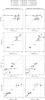 |
Fig. 18 Comparison of values found by ASteCA with those present in the SP set (articles using the same photometric system). Left column: parameters obtained using a manually fixed radius value for each OC vs. literature values. Right column: idem, except using radius values automatically assigned by ASteCA. Identity relation shown as a dashed black line. |
Ruprecht 1 stands out in Fig. 18 as it is given a large positive metallicity when rcl,a is used, larger than that assigned in its SP study, Ref. [33] (Piatti et al. 2008). This reference mentions that the cluster “might” be of solar metallicity, which is in better agreement with the values found by the code and in the DP source Ref. [19]. A similar but more pronounced behavior can be seen for NGC 2324 in Fig. 19, where it clearly separates itself from the rest of the OCs to the right of the identity line in the case of the DP article Ref. [21] (Kyeong et al. 2001), which reports [ Fe/H ] = −0.32. Both [ Fe/H ] values found by ASteCA are in good agreement with the [ Fe/H ] = 0.0 value given in the DP source Ref. [20] (Mermilliod et al. 2001), but not with that found in the SP article Ref. [22] ([ Fe/H ] = −0.3 ± 0.1, Piatti et al. 2004c). Both Czernik 26 and Czernik 30 are assigned low [ Fe/H ] values by Ref. [6] (Hasegawa et al. 2008) since they are assumed to be of subsolar metallicities given their galactocentric distances. These values show a good match with those found by ASteCA using the automatic radius, but disagree with the above-solar values derived when the manual radius was used (see Table 7).
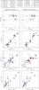 |
Fig. 19 Comparison of values found by ASteCA with those present in the DP set (articles using different photometric systems). Left column: parameters obtained using a manually fixed radius value for each OC vs. literature values. Right column: idem, except using radius values automatically assigned by ASteCA. Identity relation shown as a dashed black line. |
The uncertainties associated with the metallicities are quite large as expected, not only those obtained by ASteCA but those present in the literature as well. We warn the reader that a single CMD analysis, as that performed by the code in its current form should not replace specific and metal sensitive studies. Metallicity values returned must be be considered, along with its uncertainties, as probable ranges that should be further investigated with the right tools.
The age parameter is recovered very closely to the literature values for both sets. In the case of older clusters (log (age) > 8), two cases stand out in the SP set: Ruprecht 1 and Czernik 26, see Fig. 18. The former OC shows a larger age value, log (age) ~ 9.0, than that assigned in the literature (log (age) = 8.3; Ref [33]), but with a substantial uncertainty, almost log (age) ~ 1, for both radii values. This is a result of the cluster’s low star density, which also gives it the lowest average probability of being a true OC (~0.42). A better match is found with the value determined by the DP source Ref. [19] of log (age) = 8.76. For Czernik 26, the automatic radius found is larger than that fixed by eye resulting in a lot more field stars being added to the cluster region; the effect of this contamination is to disrupt the synthetic cluster fitting process into selecting a less than optimal model with a low positioned TO point (Fig. A.1, top row) and thus a larger age. As explained in Sect. 3.1.5 and shown in Fig. 17, this issue can be addressed by increasing the minimum MP value a star in the cluster region should have in order to affect the best model fitting algorithm (i.e., the probmin parameter). This is also the only instance where we can be completely confident that the code is producing a solution of lower quality than that present in any reference article.
The log (age) = 7.9 value given to NGC 2236 in Ref. [14] (Babu 1991) and shown in Fig. 19 is much lower than those found in the rest of the literature and those given by the code (log (age) ≥ 8.7, see Table 7). Taking into account that the EB − V extinction reported is also higher by ~0.2 than all values assigned to this cluster, we can be relatively certain that this is an example of the negative correlation effect between the Δparam of log (age) and reddening established in Sect. 3.1.4 (see Table 3). We then conclude that the age has been underestimated in this article.
For younger clusters we can mention three notable cases: NGC 2421, NGC 133, and Trumpler 1. NGC 2421 is assigned by the code an age of log (age) ≃ 7.9 in agreement with Ref. [24] but slightly larger than the values given in Ref. [19] (SP set) and Ref. [23] (McSwain & Gies 2005, DP set), where log (age) ≃ 7.41 and ≃ 7.4 are given, respectively. The cluster NGC 133, see Fig. A.1, has a low member count and a very high rate of field star contamination (CI ≃ 0.91). A single study has been performed on it, Ref. [13] (Carraro 2002), where an age of log (age) = 7 is determined, very close to the value found by the code using the automatic radius. The manual radius used is larger and includes more contaminating field stars, in particular one located around [ (B − V) = 0.7; V = 10 ]; the code recognizes this star as an evolved member of the cluster, thus resolving it as a much older system of log (age) = 9. This is accompanied by a null reddening value, in contrast with the high extinction assigned to this cluster by the reference, EB − V = 0.6, and found by the code using the automatic radius, EB − V = 0.7. Once again this is a clear consequence of the negative age-reddening correlation. The code finds Trumpler 1 to have an average age of log (age) ≃ 7.9, somewhat larger than the values given in the literature where the maximum is log (age) = 7.6 for Ref. [37] (Yadav & Sagar 2002); this age is nonetheless within the uncertainties associated with the code’s values. As seen in Fig. A.1, the match of this cluster’s upper sequence, containing the majority of probable members, with the best isochrones found by ASteCA is very good.
In the lower left corner of the age plots in Fig. 19, we can clearly appreciate the effect mentioned in Sect. 3.1.5 where very young clusters will tend to have their ages overestimated by the code. Bochum 11, see Fig. A.1, is not only a good example of this behavior, but also a demonstration of the code’s ability to perform adequately even with extremely poorly populated open clusters. Additionally, this cluster was analyzed using a V vs. (U − V) CMD to show how the code can presently take advantage of the U filter.
Reddening values obtained via ASteCA applying manual radii appear to be more dispersed when compared with those found in the literature for either set, while the values that resulted from using the automatic radii are more concentrated around the identity line for both sets of articles. Figures 18 and 19 show particularly large values for this parameter, which we derived when the manual radius was used for the case of Tombaugh 1 and NGC 2627 for the SP and DP set, and for Czernik 26 in the SP set. This discrepancy is likely due to the lower age assigned to them in this analysis, which forces the isochrone to be displaced in the CMD lower (toward larger distance modulus) and to the right (increasing reddening) to coincide with the cluster’s TO. The effect is also noticeable for the automatic radii analysis in the case of Czernik 30, as seen in Figs. 18 and A.1 (second row) and especially for NGC 133 in the manual radius analysis for the DP set, Fig. 19 left, as mentioned previously.
Trumpler 14 displays a substantial difference of 0.44 with the large EB − V = 0.84 value assigned by Ref. [41] (Ortolani et al. 2008), see Fig. 19, but a much closer match to the remaining literature values in Refs. [19] and [42] (Hur et al. 2012), which show a maximum deviation of ~0.5 as seen in Table 7. Other studies determine for this cluster values of EB − V = 0.56 ± 0.13 (Vazquez et al. 1996) and 0.57 ± 0.12 (Carraro et al. 2004, where a mean value of Rv = 4.16 is also obtained). In Yadav & Sagar (2001) the authors derive a spatial variation of reddening in the area of this cluster ranging from EB − V = 0.44 to 0.82, which would explain the discrepancies between the various values found in the literature.
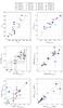 |
Fig. 20 Top: manual vs. automatic radius shown in the left diagram, and CIs obtained for the OCs with each radius in the right diagram. For clusters whose coordinates are given in degrees, their radii values were rescaled for plotting purposes. Middle: metallicity and log (age) obtained by ASteCA using each radius value. Bottom: idem above for EB − V and distance. |
Distances show on average an excellent agreement with literature values, with two apparent exceptions. The older cluster Czernik 26 is positioned ~2 kpc farther away than its SP Ref. [7] article (Piatti et al. 2009) when using the manual radius but this large distance is in perfect coincidence with the DP value, Ref. [6], of 8.9 kpc. The reason for this discrepancy is the low reddening used in Ref. [7] (EB − V = 0.05) compared with the much higher value given in Ref. [6] and found by the code with the manual radius (0.38 and 0.3, respectively), which results in a lower distance determination as the positive distance-reddening correlation indicates (see Table 3).
The second exception is the young cluster Haffner 19 (see Fig. 19) located at d ≃ 3.1 kpc, between 1.9 and 3.4 kpc closer than DP literature estimates (d = 6.4,5.2,5.1 kpc in Ref. [10], Vázquez et al. 2010; [11], Moreno-Corral et al. 2002 and [12], Munari & Carraro 1996; respectively). The age and reddening parameters obtained by the code show very similar values to those present in the three DP sources as seen in Table 7, the only difference arises in the assignment of the metal content. While ASteCA finds that this cluster is markedly metal deficient ([ Fe/H ] ≃ −1), the three articles listed as references carry out the analysis assuming solar metal content exclusively. The positive metallicity-distance correlation effect discussed earlier would indicate that this is the source of the lower distance derived by the code, or equivalently, the larger distances estimated by the other studies. Indeed, if ASteCA is run on this cluster constraining the metallicity range around a solar value of z⊙ = 0.0152, as opposed to using the entire range shown in Table 8, the resulting distance is d ≃ 4.4 kpc, much more similar to that reported in the references. If the old z⊙ = 0.019 value is used, the distance obtained is even larger: d ≃ 5.3 kpc.
Trumpler 5 is an interesting case not only because it is one of the OCs with the highest average CI value (CI ≃ 0.79), but also because no field regions could be determined when the automatic radius analysis was performed because of the large rcl,a value assigned. Field regions need to have an equal area to that of the cluster region and, in this case, the frame was not big enough to fit even one field region. With no field regions present, the DA could not be applied (field stars are necessary to calculate the MPs, see Sect. 2.8.1) so all stars within the cluster region were given equal probabilities of being true members (see Fig. A.1, ninth row, CMD on the right). The cluster parameters found by the GA are nevertheless very reasonable for both the SP and the DP sets, which means the best-fit method is robust enough to handle highly contaminated OCs even when no MPs can be obtained.
Finally, Fig. 20 shows a direct comparison between the cluster parameters obtained by ASteCA using the radii values assigned manually and automatically. The code by default attempts to include as many cluster members as possible in the cluster region (i.e., within the rcl,a boundary), so it will in general return slightly larger radii than those assigned manually, top left plot in Fig. 20. This results in higher CIs as more field stars are inevitably included in the region. For the set of OCs analyzed, the CI values are somewhat large, up to ~1 (top right plot in Fig. 20) because of the low overdensity of stars in the cluster regions (positional charts for each OC can be seen in Appendix A). The scatter around the identity line in all plots, albeit small in most cases (with the exception of the incorrect age and reddening assignment for Czernik 26 when the automatic radius was used and for NGC 133 when the manual radius was used), points to the importance of performing a careful analysis when determining the radius of an OC, especially if little information (photometric and/or kinematic) is available and the search space for the parameters is large. There is a delicate balance between a small radius that could potentially leave out defining cluster members and a radius too large that introduces substantial field star contamination, thus making the process of finding the optimal cluster parameters substantially more difficult. It is worth noting that these values are nonetheless no more scattered than those that can be found in the literature by various sources, indicating that the results returned by ASteCA using a minimal of photometric information (i.e., only two bands) are at least as good as those determined by means of methods that require involvement by the researcher and in general make use of more photometric bands, with the added advantages of objectivity and reproducibility, statistical uncertainty estimation, and full automatization.
5. Summary and conclusions
We presented ASteCA, a new set of open source tools dedicated to the study of SCs able to handle large databases both objectively and automatically. Among others, the code includes functions to perform structure analysis, LF curve, and integrated color estimations statistically cleaned from field star contamination, a Bayesian membership assignment algorithm, and a synthetic cluster-based best isochrone matching method to simultaneously estimate a cluster’s metal content and age, along with its distance and reddening. Its main objectives can be summarized as follows:
-
provide an extensible open source template software fordeveloping SC analysis tools;
-
remove the necessity to implement the frequent and inferior by-eye isochrone matching, replacing it with a powerful and easy to apply code; and
-
facilitate the automatic processing of large databases of stars with enough flexibility to encompass several scenarios, thus enabling the compilation of homogeneous catalogs of SCs.
Exhaustive tests with artificial SCs generated via the MASSCLEAN package have shown that ASteCA provides accurate parameters for clusters suffering from low or moderate field star contamination, and largely acceptable parameters for highly contaminated objects. The code introduces no biases or new correlations between the final cluster parameter values it determines. Being able to implement this internal validation makes it possible to assess the limiting resolution ASteCA can achieve when recovering parameters in any situation, provided enough SOCs can be generated and analyzed.
We obtained fundamental parameters for 20 OCs with available CT1, UBV, and 2MASS photometry. The resulting values were compared with studies using the same photometric system when available, as well as a second set of studies done using many different photometric systems. In both approaches, the resulting age, distance, and reddening estimates showed very good agreement with those from the literature, the metallicity showing a larger dispersion. The radius assigned to an OC turned out to be an important factor in estimating the cluster parameters, with small variations in its value leading to rather diverse solutions.
The ability to provide an estimate for the metallicity and its uncertainty is a crucial feature considering this is a seldom reliably obtained parameter, much less one that can be found homogeneously determined. In most studies its value is simply fixed as solar (Paunzen et al. 2010). As stated in Oliveira et al. (2013), fewer than 10% of the OCs in the DAML02 catalog have their metal contents estimated in the literature, which makes this an significant gap in the study of stellar evolution and the Galactic abundance gradient, among other fields. Although ASteCA is able to assign metallicities with an acceptable level of accuracy for OCs with low field star contamination while correctly accounting for the age-metallicity degeneracy issue, we find that this parameter is expectedly the most difficult one to obtain and the uncertainties attached to its values are by far the largest.
In general, increasing the resolution of a parameter in the search space of the best model fitting method will only lead to better results to the extent that the available photometric information permits it. It would be interesting then to investigate the increase in the attainable accuracy for the cluster parameters, in particular for the estimated metal abundance, when using larger spaces of observed data and/or different photometric systems.
Though the code is applicable to a wide range of situations, some limitations do apply. Clusters with very low member counts or high field star contamination should be treated with caution since even a single misinterpreted star can make a substantial difference, especially when determining the age. Very young clusters with no evolved stars are particularly sensitive to contamination, which can induce the code to assign larger age values by identifying bright field stars as spurious members. Regions affected by differential reddening also pose a great challenge, as the code will by default assume a unique extinction value. In all these cases it is advisable to err on the side of caution and treat returned values as first order approximations. When more information is made available, it should be used to either verify or dismiss the results. Running the code more than once with different ranges for the input parameters is a good idea.
ASteCA is meant to be considered a first step in the collaborative aim toward an objective automatization and standardization in the study of OCs. It is written entirely in Python30 (with one optional routine making use of the R statistical software package, see Sect. 2.7) and works on 2.7.x versions up to the latest 2.7.8 release, with 3.x support on the roadmap.
ASteCA is released under a general public license (GPL v331) and can be downloaded from its official site32. The code joins a growing base of recent open source astronomy and astrophysics software, which includes the set of MASSCLEAN tools, AMUSE33, AstroML (Vanderplas et al. 2012)34, and Astropy (Astropy Collaboration et al. 2013)35.
MASSive CLuster Evolution and ANalysis Package, http://www.physics.uc.edu/~bogdan/massclean/
Taken from the Canadian Astronomy Data Centre, http://www2.cadc-ccda.hia-iha.nrc-cnrc.gc.ca/
Written for the R software (http://www.r-project.org/)
“The p-value of a hypothesis test is the probability, assuming the null hypothesis is true, of observing a result at least as extreme as the value of the test statistic” (Feigelson & Babu 2012).
We refer the reader to Gallart et al. (2005) for a somewhat outdated but thorough review on the study of SFHs via the interpretation of composite stellar populations’ CMDs.
Catalogue of Open Cluster Data, available at CDS via http://cdsarc.u-strasbg.fr/viz-bin/Cat?J/A+A/438/1163
Milky Way Star Clusters, available at CDS via http://cdsarc.u-strasbg.fr/viz-bin/qcat?J/A+A/543/A156
We will not repeat the full Bayesian formalism from where this is deduced here; see the aforementioned works in Sect. 2.9 for more detail.
“The effects of increasing metal abundance on stellar isochrones are remarkably similar to those of increasing age” (Frayn & Gilmore 2003).
The total mass value Mtotal is fixed for all synthetic clusters generated by the method, so we set it to a number high enough to ensure the evolved parts of the isochrone are also sampled. We plan on removing this restriction in a future version of the code so that this can be left as an extra free parameter to be fitted by the method.
More details about the algorithm can be found in the code’s documentation, see: http://asteca.rtfd.org
The complete set of SOCs is available upon request. The scripts used to generate the set can be obtained via: https://github.com/Gabriel-p/massclean_cl
This comes from the fact that the CI can be written as: CI = nfl/ (nfl + ncl) where nfl and ncl are the number of field and cluster member stars expected within the cluster region, respectively (see Eq. (2)). If CI = 0.7, we get from the previous relation: nfl = 2.3 ncl.
We made use of the WEBDA database (accessible at http://www.univie.ac.at/webda/) to retrieve the photometry for these clusters.
ASteCA: http://http://asteca.github.io/
Astrophysical Multipurpose Software Environment: http://www.amusecode.org/
Machine Learning and Data Mining for Astronomy: http://www.astroml.org/
Community-developed core Python package for Astronomy: http://www.astropy.org/
Acknowledgments
G. I. Perren is very grateful to Drs. Girardi L., Popescu B., Moitinho A., Hernandez X., Kharchenko N., Dias W., Bonatto C., and Duong T. for the valuable input provided during the preparation of this article. Authors are very much indebted with Dr E. V. Glushkova for the helpful comments and constructive suggestions that contributed to greatly improve the manuscript. The authors express their gratitude to the Universidad de La Plata and Universidad de Córdoba. G. I. Perren and R. A. Vázquez acknowledge the financial support from the CONICET PIP1359. This work was partially supported by the Argentinian institutions CONICET and Agencia Nacional de Promoción Científica y Tecnológica (ANPCyT). This publication makes use of data products from the Two Micron All-Sky Survey, which is a joint project of the University of Massachusetts and the Infrared Processing and Analysis Center/California Institute of Technology, funded by the National Aeronautics and Space Administration and the National Science Foundation. This research has made use of the WEBDA database, operated at the Department of Theoretical Physics and Astrophysics of the Masaryk University.
References
- Ahumada, J. A. 2005, Astron. Nachr., 326, 3 [NASA ADS] [CrossRef] [Google Scholar]
- Alves, V., Pavani, D., Kerber, L., & Bica, E. 2012, New Astron., 17, 488 [NASA ADS] [CrossRef] [Google Scholar]
- An, D., Terndrup, D. M., Pinsonneault, M. H., et al. 2007, ApJ, 655, 233 [NASA ADS] [CrossRef] [Google Scholar]
- Anders, P., Bissantz, N., Fritze-v. Alvensleben, U., & de Grijs, R. 2004, MNRAS, 347, 196 [NASA ADS] [CrossRef] [Google Scholar]
- Aparicio, A., & Hidalgo, S. L. 2009, AJ, 138, 558 [NASA ADS] [CrossRef] [MathSciNet] [Google Scholar]
- Astropy Collaboration, Robitaille, T. P., Tollerud, E. J., et al. 2013, A&A, 558, A33 [NASA ADS] [CrossRef] [EDP Sciences] [Google Scholar]
- Baade, D. 1983, A&AS, 51, 235 [NASA ADS] [Google Scholar]
- Babu, G. S. D. 1991, JA&A, 12, 187 [NASA ADS] [Google Scholar]
- Balaguer-Nunez, L., Jordi, C., Galadi-Enriquez, D., & Zhao, J. L. 2004, A&A, 426, 819 [NASA ADS] [CrossRef] [EDP Sciences] [Google Scholar]
- Beaver, J., Kaltcheva, N., Briley, M., & Piehl, D. 2013, PASP, 125, 1412 [NASA ADS] [CrossRef] [Google Scholar]
- Bica, E., & Bonatto, C. 2005, A&A, 443, 465 [NASA ADS] [CrossRef] [EDP Sciences] [Google Scholar]
- Bica, E., Bonatto, C., Dutra, C. M., & Santos, J. F. C. 2008, MNRAS, 389, 678 [NASA ADS] [CrossRef] [Google Scholar]
- Bonatto, C., & Bica, E. 2005, A&A, 437, 483 [NASA ADS] [CrossRef] [EDP Sciences] [Google Scholar]
- Bonatto, C., & Bica, E. 2007, MNRAS, 377, 1301 [NASA ADS] [CrossRef] [Google Scholar]
- Bonatto, C., & Bica, E. 2009, MNRAS, 392, 483 [NASA ADS] [CrossRef] [Google Scholar]
- Bressan, A., Marigo, P., Girardi, L., et al. 2012, MNRAS, 427, 127 [NASA ADS] [CrossRef] [Google Scholar]
- Bressan, A., Marigo, P., Girardi, L., Nanni, A., & Rubele, S. 2013, EPJ Web Conf., 43, 03001 [CrossRef] [EDP Sciences] [Google Scholar]
- Buckner, A. S. M., & Froebrich, D. 2013, MNRAS, 436, 1465 [NASA ADS] [CrossRef] [Google Scholar]
- Buckner, A. S. M., & Froebrich, D. 2014, MNRAS, 444, 290 [NASA ADS] [CrossRef] [Google Scholar]
- Bukowiecki, Ł., Maciejewski, G., Konorski, P., & Strobel, A. 2011, Acta Astron., 61, 231 [NASA ADS] [Google Scholar]
- Cabrera-Cano, J., & Alfaro, E. J. 1990, A&A, 235, 94 [NASA ADS] [Google Scholar]
- Cantat-Gaudin, T., Vallenari, A., Zaggia, S., et al. 2014, A&A, 569, A17 [NASA ADS] [CrossRef] [EDP Sciences] [Google Scholar]
- Canterna, R. 1976, AJ, 81, 228 [NASA ADS] [CrossRef] [Google Scholar]
- Carraro, G. 2002, A&A, 387, 479 [NASA ADS] [CrossRef] [EDP Sciences] [Google Scholar]
- Carraro, G., & Patat, F. 1995, MNRAS, 276, 563 [NASA ADS] [CrossRef] [Google Scholar]
- Carraro, G., Girardi, L., & Marigo, P. 2002, MNRAS, 332, 705 [NASA ADS] [CrossRef] [Google Scholar]
- Carraro, G., Romaniello, M., Ventura, P., & Patat, F. 2004, A&A, 418, 525 [NASA ADS] [CrossRef] [EDP Sciences] [Google Scholar]
- Carraro, G., Beletsky, Y., & Marconi, G. 2013, MNRAS, 428, 502 [NASA ADS] [CrossRef] [Google Scholar]
- Carraro, G., Giorgi, E. E., Costa, E., & Vazquez, R. A. 2014, MNRAS, 441, L36 [NASA ADS] [CrossRef] [Google Scholar]
- Cerviño, M., Pérez, E., Sánchez, N., Román-Zúñiga, C., & Valls-Gabaud, D. 2011, in UP2010: Have Observations Revealed a Variable Upper End of the Initial Mass Function?, eds. M. Treyer, T. Wyder, J. Neill, M. Seibert, & J. Lee, ASP Conf. Ser., 440, 133 [Google Scholar]
- Chabrier, G. 2001, ApJ, 554, 1274 [NASA ADS] [CrossRef] [Google Scholar]
- Charbonneau, P. 1995, ApJSS, 101, 309 [NASA ADS] [CrossRef] [Google Scholar]
- Chiosi, C., Bertelli, G., Meylan, G., & Ortolani, S. 1989, A&A, 219, 167 [NASA ADS] [Google Scholar]
- Cignoni, M., Beccari, G., Bragaglia, A., & Tosi, M. 2011, MNRAS, 416, 1077 [NASA ADS] [CrossRef] [Google Scholar]
- Claria, J. J., & Lapasset, E. 1986, AJ, 91, 326 [NASA ADS] [CrossRef] [Google Scholar]
- Claria, J. J., Piatti, A. E., Parisi, M. C., & Ahumada, A. V. 2007, MNRAS, 379, 159 [NASA ADS] [CrossRef] [Google Scholar]
- Dahm, S. E., Simon, T., Proszkow, E. M., & Patten, B. M. 2007, AJ, 134, 999 [NASA ADS] [CrossRef] [Google Scholar]
- de Grijs, R., Anders, P., Lamers, H. J. G. L. M., et al. 2005, MNRAS, 359, 874 [NASA ADS] [CrossRef] [Google Scholar]
- de Meulenaer, P., Narbutis, D., Mineikis, T., & Vansevičius, V. 2013, A&A, 550, A20 [NASA ADS] [CrossRef] [EDP Sciences] [Google Scholar]
- Dias, W. S., Alessi, B. S., Moitinho, A., & Lepine, J. R. D. 2002, A&A, 389, 871 [NASA ADS] [CrossRef] [EDP Sciences] [Google Scholar]
- Dias, W. S., Monteiro, H., Caetano, T. C., & Oliveira, A. F. 2012, A&A, 539, A125 [NASA ADS] [CrossRef] [EDP Sciences] [Google Scholar]
- Dias, B., Kerber, L. O., Barbuy, B., et al. 2014, A&A, 561, A106 [NASA ADS] [CrossRef] [EDP Sciences] [Google Scholar]
- Dolphin, A. E. 2002, MNRAS, 332, 91 [NASA ADS] [CrossRef] [Google Scholar]
- Donati, P., Beccari, G., Bragaglia, A., Cignoni, M., & Tosi, M. 2014, MNRAS, 437, 1241 [NASA ADS] [CrossRef] [Google Scholar]
- Duong, T. 2007, J. Statistical Software, 21, 1 [Google Scholar]
- Duong, T., Goud, B., & Schauer, K. 2012, Proc. Nat. Acad. Sci., 109, 8382 [NASA ADS] [CrossRef] [Google Scholar]
- Feigelson, E. D., & Babu, G. J. 2012, Mod. Statistic. Meth. Astron. (Cambridge University Press) [Google Scholar]
- Ferraro, F. R., Fusi Pecci, F., Tosi, M., & Buonanno, R. 1989, MNRAS, 241, 433 [NASA ADS] [CrossRef] [Google Scholar]
- Fitzgerald, M. P., & Mehta, S. 1987, MNRAS, 228, 545 [NASA ADS] [CrossRef] [Google Scholar]
- Fouesneau, M., & Lançon, A. 2010, A&A, 521, A22 [NASA ADS] [CrossRef] [EDP Sciences] [Google Scholar]
- Frayn, C. M., & Gilmore, G. F. 2002, MNRAS, 337, 445 [NASA ADS] [CrossRef] [Google Scholar]
- Frayn, C. M., & Gilmore, G. F. 2003, MNRAS, 339, 887 [NASA ADS] [CrossRef] [Google Scholar]
- Frinchaboy, P. M., & Majewski, S. R. 2008, AJ, 136, 118 [NASA ADS] [CrossRef] [Google Scholar]
- Froebrich, D., Scholz, A., & Raftery, C. L. 2007, MNRAS, 374, 399 [Google Scholar]
- Froebrich, D., Schmeja, S., Samuel, D., & Lucas, P. W. 2010, MNRAS, 409, 1281 [NASA ADS] [CrossRef] [Google Scholar]
- Gallart, C., Zoccali, M., & Aparicio, A. 2005, ARA&A, 43, 387 [NASA ADS] [CrossRef] [Google Scholar]
- Geisler, D., Lee, M. G., & Kim, E. 1996, AJ, 111, 1529 [NASA ADS] [CrossRef] [Google Scholar]
- Girardi, L., Bressan, A., Bertelli, G., & Chiosi, C. 2000, A&AS, 141, 371 [NASA ADS] [CrossRef] [EDP Sciences] [Google Scholar]
- Girardi, L., Rubele, S., & Kerber, L. 2009, MNRAS, 394, L74 [NASA ADS] [Google Scholar]
- Girardi, L., Williams, B. F., Gilbert, K. M., et al. 2010, ApJ, 724, 1030 [NASA ADS] [CrossRef] [Google Scholar]
- Gray, F. D. 1965, AJ, 70, 362 [NASA ADS] [CrossRef] [Google Scholar]
- Hasegawa, T., Sakamoto, T., & Malasan, H. L. 2008, PASJ, 60, 1267 [NASA ADS] [CrossRef] [Google Scholar]
- Hernandez, X., & Valls-Gabaud, D. 2008, MNRAS, 383, 1603 [NASA ADS] [CrossRef] [Google Scholar]
- Hernandez, X., Valls-Gabaud, D., & Gilmore, G. 1999, MNRAS, 304, 705 [NASA ADS] [CrossRef] [Google Scholar]
- Hillenbrand, L. A., & Hartmann, L. W. 1998, AJ, 492, 540 [Google Scholar]
- Hur, H., Sung, H., & Bessell, M. S. 2012, AJ, 143, 41 [NASA ADS] [CrossRef] [Google Scholar]
- Janes, K. 2001, The Encyclopedia of Astronomy and Astrophysics [Google Scholar]
- Javakhishvili, G., Kukhianidze, V., Todua, M., & Inasaridze, R. 2006, A&A, 447, 915 [NASA ADS] [CrossRef] [EDP Sciences] [Google Scholar]
- Kaluzny, J. 1998, A&AS, 133, 25 [NASA ADS] [CrossRef] [EDP Sciences] [Google Scholar]
- Kerber, L. O., & Santiago, B. X. 2005, A&A, 435, 77 [NASA ADS] [CrossRef] [EDP Sciences] [Google Scholar]
- Kerber, L. O., Santiago, B. X., Castro, R., & Valls-Gabaud, D. 2002, A&A, 390, 121 [NASA ADS] [CrossRef] [EDP Sciences] [Google Scholar]
- Kerber, L. O., Santiago, B. X., & Brocato, E. 2007, A&A, 462, 139 [NASA ADS] [CrossRef] [EDP Sciences] [Google Scholar]
- Kharchenko, N. V., Piskunov, A. E., Röser, S., Schilbach, E., & Scholz, R.-D. 2005a, A&A, 440, 403 [NASA ADS] [CrossRef] [EDP Sciences] [Google Scholar]
- Kharchenko, N. V., Piskunov, A. E., Röser, S., Schilbach, E., & Scholz, R.-D. 2005b, A&A, 438, 1163 [NASA ADS] [CrossRef] [EDP Sciences] [MathSciNet] [Google Scholar]
- Kharchenko, N. V., Piskunov, A. E., Schilbach, E., Röser, S., & Scholz, R.-D. 2013, A&A, 558, A53 [NASA ADS] [CrossRef] [EDP Sciences] [Google Scholar]
- King, I. 1962, AJ, 67, 471 [NASA ADS] [CrossRef] [Google Scholar]
- Koornneef, J. 1983, A&A, 128, 84 [NASA ADS] [Google Scholar]
- Kozhurina-Platais, V., Girard, T. M., Platais, I., et al. 1995, AJ, 109, 672 [NASA ADS] [CrossRef] [Google Scholar]
- Krone-Martins, A., & Moitinho, A. 2014, A&A, 561, A57 [NASA ADS] [CrossRef] [EDP Sciences] [Google Scholar]
- Krone-Martins, A., Soubiran, C., Ducourant, C., Teixeira, R., & Le Campion, J. F. 2010, A&A, 516, A3 [NASA ADS] [CrossRef] [EDP Sciences] [Google Scholar]
- Kroupa, P. 2002, Science, 295, 82 [NASA ADS] [CrossRef] [PubMed] [Google Scholar]
- Kroupa, P., Tout, C. A., & Gilmore, G. 1993, MNRAS, 262, 545 [NASA ADS] [CrossRef] [Google Scholar]
- Kyeong, J.-M., Byun, Y.-I., & Sung, E.-C. 2001, J. Korean Astron. Soc., 34, 143 [Google Scholar]
- Lata, S., Pandey, A. K., Sharma, S., Bonatto, C., & Yadav, R. K. 2014, New A, 26, 77 [NASA ADS] [CrossRef] [Google Scholar]
- Maciejewski, G., & Niedzielski, A. 2007, A&A, 467, 1065 [NASA ADS] [CrossRef] [EDP Sciences] [Google Scholar]
- Maia, F. F. S., Corradi, W. J. B., & Santos, Jr J. F. C. 2010, MNRAS, 407, 1875 [NASA ADS] [CrossRef] [Google Scholar]
- Maia, F. F. S., Piatti, A. E., & Santos, J. F. C. 2014, MNRAS, 437, 2005 [NASA ADS] [CrossRef] [Google Scholar]
- Majaess, D., Turner, D., Bidin, C. M., et al. 2012, A&A, 537, L4 [NASA ADS] [CrossRef] [EDP Sciences] [Google Scholar]
- Marigo, P., Girardi, L., Bressan, A., et al. 2008, A&A, 482, 883 [NASA ADS] [CrossRef] [EDP Sciences] [Google Scholar]
- Mateo, M., & Hodge, P. 1986, ApJS, 60, 893 [NASA ADS] [CrossRef] [Google Scholar]
- McSwain, M. V., & Gies, D. R. 2005, ApJS, 161, 118 [NASA ADS] [CrossRef] [Google Scholar]
- Mermilliod, J.-C., Clariá, J. J., Andersen, J., Piatti, A. E., & Mayor, M. 2001, A&A, 375, 30 [NASA ADS] [CrossRef] [EDP Sciences] [Google Scholar]
- Mighell, K. J., Rich, R. M., Shara, M., & Fall, S. M. 1996, AJ, 111, 2314 [NASA ADS] [CrossRef] [Google Scholar]
- Moffat, A. F. J., & Vogt, N. 1975, A&AS, 20, 125 [NASA ADS] [Google Scholar]
- Monteiro, H., Dias, W. S., & Caetano, T. C. 2010, A&A, 516, A2 [NASA ADS] [CrossRef] [EDP Sciences] [Google Scholar]
- Moreno-Corral, M. A., Chavarría-K., C., & de Lara, E. 2002, Rev. Mex. Astron. Astrofis., 38, 141 [NASA ADS] [Google Scholar]
- Munari, U., & Carraro, G. 1996, MNRAS, 283, 905 [NASA ADS] [Google Scholar]
- Oliveira, A. F., Monteiro, H., Dias, W. S., & Caetano, T. C. 2013, A&A, 557, A14 [NASA ADS] [CrossRef] [EDP Sciences] [Google Scholar]
- Ortolani, S., Bonatto, C., Bica, E., Momany, Y., & Barbuy, B. 2008, New Astron., 13, 508 [Google Scholar]
- Ozsvath, I. 1960, Astronomische Abhandlungen der Hamburger Sternwarte, 5, 129 [NASA ADS] [Google Scholar]
- Patat, F., & Carraro, G. 2001, MNRAS, 325, 1591 [NASA ADS] [CrossRef] [Google Scholar]
- Paunzen, E., Netopil, M., & Zwintz, K. 2007, A&A, 462, 157 [NASA ADS] [CrossRef] [EDP Sciences] [Google Scholar]
- Paunzen, E., Heiter, U., Netopil, M., & Soubiran, C. 2010, A&A, 517, A32 [NASA ADS] [CrossRef] [EDP Sciences] [Google Scholar]
- Pavani, D. B., & Bica, E. 2007, A&A, 468, 139 [NASA ADS] [CrossRef] [EDP Sciences] [Google Scholar]
- Pavani, D. B., Kerber, L. O., Bica, E., & Maciel, W. J. 2011, MNRAS, 412, 1611 [NASA ADS] [CrossRef] [Google Scholar]
- Phelps, R. L., & Janes, K. A. 1994, ApJS, 90, 31 [NASA ADS] [CrossRef] [Google Scholar]
- Phelps, R. L., Janes, K. A., & Montgomery, K. A. 1994, AJ, 107, 1079 [NASA ADS] [CrossRef] [Google Scholar]
- Piatti, A. E., & Bica, E. 2012, MNRAS, 425, 3085 [NASA ADS] [CrossRef] [Google Scholar]
- Piatti, A. E., Clariá, J. J., & Ahumada, A. V. 2003, MNRAS, 346, 390 [NASA ADS] [CrossRef] [Google Scholar]
- Piatti, A. E., Clariá, J. J., & Ahumada, A. V. 2004a, A&A, 421, 991 [NASA ADS] [CrossRef] [EDP Sciences] [Google Scholar]
- Piatti, A. E., Clariá, J. J., & Ahumada, A. V. 2004b, MNRAS, 349, 641 [NASA ADS] [CrossRef] [Google Scholar]
- Piatti, A. E., Clariá, J. J., & Ahumada, A. V. 2004c, A&A, 418, 979 [NASA ADS] [CrossRef] [EDP Sciences] [Google Scholar]
- Piatti, A. E., Clariá, J. J., Parisi, M. C., & Ahumada, A. V. 2008, Balt. Astron., 17, 67 [NASA ADS] [Google Scholar]
- Piatti, A. E., Clariá, J. J., Parisi, M. C., & Ahumada, A. V. 2009, New A, 14, 97 [NASA ADS] [CrossRef] [Google Scholar]
- Piskunov, A. E., Schilbach, E., Kharchenko, N. V., Röser, S., & Scholz, R.-D. 2007, A&A, 468, 151 [NASA ADS] [CrossRef] [EDP Sciences] [Google Scholar]
- Pöhnl, H., & Paunzen, E. 2010, A&A, 514, A81 [NASA ADS] [CrossRef] [EDP Sciences] [Google Scholar]
- Popescu, B., & Hanson, M. M. 2009, AJ, 138, 1724 [NASA ADS] [CrossRef] [Google Scholar]
- Popescu, B., Hanson, M. M., & Elmegreen, B. G. 2012, ApJ, 751, 122 [NASA ADS] [CrossRef] [Google Scholar]
- Rauw, G., Manfroid, J., & De Becker, M. 2010, A&A, 511, A25 [NASA ADS] [CrossRef] [EDP Sciences] [Google Scholar]
- Roberts, L. C., Gies, D. R., Parks, J. R., et al. 2010, AJ, 140, 744 [NASA ADS] [CrossRef] [Google Scholar]
- Romeo, G., Fusi Pecci, F., Bonifazi, A., & Tosi, M. 1989, MNRAS, 240, 459 [NASA ADS] [CrossRef] [Google Scholar]
- Sánchez, N., Vicente, B., & Alfaro, E. J. 2010, A&A, 510, A78 [NASA ADS] [CrossRef] [EDP Sciences] [Google Scholar]
- Sanders, W. L. 1971, A&A, 14, 226 [NASA ADS] [Google Scholar]
- Sandrelli, S., Bragaglia, A., Tosi, M., & Marconi, G. 1999, MNRAS, 309, 739 [NASA ADS] [CrossRef] [Google Scholar]
- Santos, Jr., J. F. C., Bonatto, C., & Bica, E. 2005, A&A, 442, 201 [NASA ADS] [CrossRef] [EDP Sciences] [Google Scholar]
- Sarro, L. M., Bouy, H., Berihuete, A., et al. 2014, A&A, 563, A45 [NASA ADS] [CrossRef] [EDP Sciences] [Google Scholar]
- Schmeja, S., Kharchenko, N. V., Piskunov, A. E., et al. 2014, A&A, 568, A51 [CrossRef] [EDP Sciences] [Google Scholar]
- Scott, D. W. 1992, Multivariate Density Estimation (John Wiley & Sons Inc.) [Google Scholar]
- Singh Kalirai, J. 2006, BASI, 34, 141 [NASA ADS] [Google Scholar]
- Skrutskie, M. F., Cutri, R. M., Stiening, R., et al. 2006, AJ, 131, 1163 [NASA ADS] [CrossRef] [Google Scholar]
- Small, E. E., Bersier, D., & Salaris, M. 2013, MNRAS, 428, 763 [NASA ADS] [CrossRef] [Google Scholar]
- Stetson, P. B. 1980, AJ, 85, 387 [NASA ADS] [CrossRef] [Google Scholar]
- Subramaniam, A., Sahu, D. K., Sagar, R., & Vijitha, P. 2005, A&A, 440, 511 [NASA ADS] [CrossRef] [EDP Sciences] [Google Scholar]
- Sung, H., Sana, H., & Bessell, M. S. 2013, AJ, 145, 37 [NASA ADS] [CrossRef] [Google Scholar]
- Tadross, A. 2001, New Astron., 6, 293 [Google Scholar]
- Tadross, A. L. 2003, New Astron., 8, 737 [NASA ADS] [CrossRef] [Google Scholar]
- Tolstoy, E., & Saha, A. 1996, ApJ, 462, 672 [Google Scholar]
- Tosi, M., Greggio, L., Marconi, G., & Focardi, P. 1991, AJ, 102, 951 [NASA ADS] [CrossRef] [Google Scholar]
- Turner, D. G. 1983, JRASC, 77, 31 [Google Scholar]
- Turner, D. G. 2012, Astron. Nachri., 333, 174 [Google Scholar]
- van Dyk, D. A., DeGennaro, S., Stein, N., Jefferys, W. H., & von Hippel, T. 2009, Ann. Appl. Stat., 3, 117 [NASA ADS] [CrossRef] [Google Scholar]
- Vanderplas, J., Connolly, A., Ivezić, Ž., & Gray, A. 2012, in Conference on Intelligent Data Understanding (CIDU), 47 [Google Scholar]
- Vasilevskis, S., Klemola, A., & Preston, G. 1958, AJ, 63, 387 [NASA ADS] [CrossRef] [Google Scholar]
- Vazquez, R. A., Baume, G., Feinstein, A., & Prado, P. 1996, A&AS, 116, 75 [NASA ADS] [Google Scholar]
- Vázquez, R. A., Moitinho, A., Carraro, G., & Dias, W. S. 2010, A&A, 511, A38 [NASA ADS] [CrossRef] [EDP Sciences] [Google Scholar]
- von Hippel, T. 2005, ApJ, 622, 565 [NASA ADS] [CrossRef] [Google Scholar]
- von Hippel, T., Jefferys, W. H., Scott, J., et al. 2006, ApJ, 645, 1436 [NASA ADS] [CrossRef] [Google Scholar]
- Whitley, D. 1994, Statistics and Computing, 4 [Google Scholar]
- Wu, Z. Y., Tian, K. P., Balaguer-Nunez, L., et al. 2002, A&A, 381, 464 [NASA ADS] [CrossRef] [EDP Sciences] [Google Scholar]
- Yadav, R. K. S., & Sagar, R. 2001, MNRAS, 328, 370 [NASA ADS] [CrossRef] [Google Scholar]
- Yadav, R. K. S., & Sagar, R. 2002, MNRAS, 337, 133 [NASA ADS] [CrossRef] [Google Scholar]
- Yadav, R. K. S., & Sagar, R. 2004, MNRAS, 351, 667 [NASA ADS] [CrossRef] [Google Scholar]
- Zhao, J. L., & He, Y. P. 1990, A&A, 237, 54 [NASA ADS] [Google Scholar]
Appendix A: Observed OCs
Figure A.1 shows for the set of real OCs analyzed, one row per OC, the following plots: positional chart (first column), observed CMD with MPs coloring generated using the manual radius value (second column), CMD of the best synthetic cluster match found by the code for the cluster region determined by the manual radius value (third column), equivalent CMDs but generated using the automatic radius value found (fourth and fifth columns).
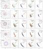 |
Fig. A.1 Diagrams for observed OCs analyzed with ASteCA displayed in rows for radii values assigned both manually (rcl,m) and automatically by the code (rcl,a). Leftmost plot is the star chart of the OC with rcl,m and rcl,a shown as blue and red circles, respectively. Second and third plots are the observed cluster region CMD (colored according to the MPs obtained by the DA) and best synthetic cluster found by the best-fit algorithm (see Sect. 2.9.1), respectively, using the rcl,m radius. Fourth and fifth plots are the same as the previous two, except using the rcl,a radius. Cluster parameters and their uncertainties can be seen in the top right of the best synthetic cluster CMDs and are summarized in Table 7. |
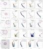 |
Fig. A.1 continued. |
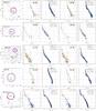 |
Fig. A.1 continued. |
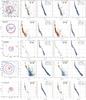 |
Fig. A.1 continued. |
All Tables
Number of poorly populated (Nmemb ≤ 50) SOCs that had their parameters recovered with relative errors (er) below the given thresholds; percentage of total sample (82) is shown in parenthesis.
All Figures
|
Fig. 1 Left: finding chart of an example artificial MASSCLEAN cluster embedded in a field of stars. Right: center determination via a two-dimensional KDE. |
| In the text | |
|
Fig. 2 Radial density profile of cluster region. Black dots are the stars /px2 RDP points taking the cluster center as the origin; the horizontal blue line is the field density value dfield, as indicated in Sect. 2.2.2; the red arrow marks the assigned radius with the uncertainty region marked as a gray shaded area; a 2P King profile fit is indicated with the green broken curve with the rcore (core radius) value shows as a vertical green line. |
| In the text | |
|
Fig. 3 Top: maximum error rejection method (left) and exponential curve method (right). Bottom: “eye fit” method. Rejected stars are shown as green crosses, and the horizontal dashed red line is the maximum error value accepted. See text for details. |
| In the text | |
|
Fig. 4 Left: cluster region centered in the frame and 15 field regions of equal area defined around it. Adjacent field stars with the same color belong to the same field region (notice that only four colors are used and they start repeating themselves in a cycle). Right: CMD showing the cluster region stars as red points, stars in the combined surrounding field regions in gray, and rejected stars by the error rejection function as green crosses. |
| In the text | |
|
Fig. 5 Left: LF curves for the cluster region plus field star contamination (red), averaged field regions scaled to the cluster’s area (blue), and clean cluster region (green); completeness limit shown as a dashed black line. Right: integrated magnitudes versus magnitude values for the cluster region (plus field star contamination) in red and average field regions in blue. |
| In the text | |
|
Fig. 6 Left: function applied on a synthetic cluster. The curves are clearly separated with the blue curve (cluster vs. field regions CMD analysis) showing much lower values; the final probability value obtained is close to 1 (or 100%). Right: same analysis performed on a random field region; the curves are now quite similar, resulting in a very low probability of the region containing a true stellar cluster. |
| In the text | |
|
Fig. 7 Top: distribution of MPs (left), probmin is the value that separates the upper half of stars with the highest MPs from the lower half and spatial chart (right) with stars in the cluster region colored by their MPs. Bottom: CMD of the observed cluster region (left) with rejected stars marked as green crosses and the same CMD minus the rejected stars (right) with coloring according to each star’s MPs. |
| In the text | |
|
Fig. 8 Generation of a synthetic cluster starting from a theoretical isochrone of fixed parameters (metallicity, age, distance, and extinction) populated using the exponential IMF of Chabrier (2001). See text for a description of each panel. |
| In the text | |
|
Fig. 9 Results of the GA applied over an example OC. See text for more details. |
| In the text | |
|
Fig. 10 Top: spatial distribution (left) of a SOC according to the parameters labeled in the respective CMD (right), wherein the green line indicates the magnitude limit adopted in the validation. Red symbols refer to cluster stars. Middle: photometric errors (left) and the completeness function (right) adopted. Bottom: resulting cluster star spatial distribution (left) with a circle representing the tidal radius and the corresponding CMD (right). |
| In the text | |
|
Fig. 11 Examples of SOCs produced as described in Sect. 3 with fixed metallicity and age, and varying total mass, distance, and visual absorption values. Symbols as in Fig. 10 (bottom panels). |
| In the text | |
|
Fig. 12 Left: logarithm of the CI vs. difference in center assigned by ASteCA with true center. Sizes vary according to the initial masses (larger mean larger initial mass) and colors according to the distance (see colorbar to the right). Right: logarithm of the CI vs. radius difference (ASteCA minus true value) for each SOC. In both plots shaded regions mark the range where 50% of all SOCs are positioned and estimated errors are shown as gray lines. |
| In the text | |
|
Fig. 13 Left: distribution of real cluster probabilities vs. CI. Sizes vary according to the initial masses (bigger size means larger initial mass) and colors according to the distance (see colorbar to the right). Circles represent values for SOCs and diamonds values obtained for field regions. Right: logarithm of the CI vs. relative error for the true number of members and that predicted by ASteCA for each SOC. Point markers are associated with ages as shown in the legend. The shaded region marks the range where 50% of all SOCs are positioned. |
| In the text | |
|
Fig. 14 Top left: member index defined in Eq. (19) vs. contamination index. Top right: same MI vs. CI plot except using the membership probabilities given by the random assignment algorithm. Bottom left: member index defined in Eq. (20) vs. contamination index. Bottom right: same MI vs. CI plot except using the membership probabilities given by the random assignment algorithm. Linear fits in each plot shown as dashed black lines. Sizes, shapes, and colors as in Fig. 12. |
| In the text | |
|
Fig. 15 Top left: metallicity differences in the sense true value minus ASteCA estimate vs. log (CI) with errors assigned by the code as gray horizontal lines. Top right: idem for log (age). Bottom left: idem for distance in kpc. Bottom right: idem for EB − V extinction. Shaded regions mark the ranges where 50% of all SOCs are positioned. Sizes, shapes, and colors as in Fig. 12. |
| In the text | |
|
Fig. 16 Left: CMD of cluster region for a MASSCLEAN young SOC with MPs for each star shown according to the color bar at the top and the best-fit isochrone found shown in green. True age value is log (age) = 7.0. Right: best-fit synthetic cluster found along with the theoretical isochrone used to generate it in red. Cluster parameters and uncertainties shown in the top right box. |
| In the text | |
|
Fig. 17 Left column: top, MPs distribution for an old SOC where the cut is done for a value of probmin = 0.75; center, CMD of cluster region with MPs for each star shown according to the color bar at the top and the best-fit isochrone found shown in green; bottom, best-fit synthetic cluster found along with the theoretical isochrone used to generate it in red, cluster parameters and uncertainties shown in the top right box. Right column: top, idem above with probability cut now done at probmin = 0.85; center, idem above with new best-fit isochrone; bottom, idem above showing new synthetic cluster and improved cluster parameters. |
| In the text | |
|
Fig. 18 Comparison of values found by ASteCA with those present in the SP set (articles using the same photometric system). Left column: parameters obtained using a manually fixed radius value for each OC vs. literature values. Right column: idem, except using radius values automatically assigned by ASteCA. Identity relation shown as a dashed black line. |
| In the text | |
|
Fig. 19 Comparison of values found by ASteCA with those present in the DP set (articles using different photometric systems). Left column: parameters obtained using a manually fixed radius value for each OC vs. literature values. Right column: idem, except using radius values automatically assigned by ASteCA. Identity relation shown as a dashed black line. |
| In the text | |
|
Fig. 20 Top: manual vs. automatic radius shown in the left diagram, and CIs obtained for the OCs with each radius in the right diagram. For clusters whose coordinates are given in degrees, their radii values were rescaled for plotting purposes. Middle: metallicity and log (age) obtained by ASteCA using each radius value. Bottom: idem above for EB − V and distance. |
| In the text | |
|
Fig. A.1 Diagrams for observed OCs analyzed with ASteCA displayed in rows for radii values assigned both manually (rcl,m) and automatically by the code (rcl,a). Leftmost plot is the star chart of the OC with rcl,m and rcl,a shown as blue and red circles, respectively. Second and third plots are the observed cluster region CMD (colored according to the MPs obtained by the DA) and best synthetic cluster found by the best-fit algorithm (see Sect. 2.9.1), respectively, using the rcl,m radius. Fourth and fifth plots are the same as the previous two, except using the rcl,a radius. Cluster parameters and their uncertainties can be seen in the top right of the best synthetic cluster CMDs and are summarized in Table 7. |
| In the text | |
|
Fig. A.1 continued. |
| In the text | |
|
Fig. A.1 continued. |
| In the text | |
|
Fig. A.1 continued. |
| In the text | |
Current usage metrics show cumulative count of Article Views (full-text article views including HTML views, PDF and ePub downloads, according to the available data) and Abstracts Views on Vision4Press platform.
Data correspond to usage on the plateform after 2015. The current usage metrics is available 48-96 hours after online publication and is updated daily on week days.
Initial download of the metrics may take a while.