| Issue |
A&A
Volume 563, March 2014
|
|
|---|---|---|
| Article Number | A112 | |
| Number of page(s) | 14 | |
| Section | The Sun | |
| DOI | https://doi.org/10.1051/0004-6361/201322476 | |
| Published online | 18 March 2014 | |
Horizontal flow fields observed in Hinode G-band images
IV. Statistical properties of the dynamical environment around pores
1 Leibniz-Institut für Astrophysik Potsdam (AIP), an der Sternwarte 16, 14482 Potsdam, Germany
e-mail: cdenker@aip.de
2 Max-Planck-Institut für Sonnensystemforschung, Max-Planck-Straße 2, 37191 Katlenburg-Lindau, Germany
e-mail: verma@mps.mpg.de
Received: 12 August 2013
Accepted: 16 January 2014
Context. Solar pores are penumbra-lacking magnetic features, that mark two important transitions in the spectrum of magnetohydrodynamic processes: (1) the magnetic field becomes sufficiently strong to suppress the convective energy transport and (2) at some critical point some pores develop a penumbra and become sunspots.
Aims. The purpose of this statistical study is to comprehensively describe solar pores in terms of their size, perimeter, shape, photometric properties, and horizontal proper motions. The seeing-free and uniform data of the Japanese Hinode mission provide an opportunity to compare flow fields in the vicinity of pores in different environments and at various stages of their evolution.
Methods. The extensive database of high-resolution G-band images observed with the Hinode Solar Optical Telescope (SOT) is a unique resource to derive statistical properties of pores using advanced digital image processing techniques. The study is based on two data sets: (1) photometric and morphological properties inferred from single G-band images cover almost seven years from 2006 October 25 to 2013 August 31; and (2) horizontal flow fields derived from 356 one-hour sequences of G-band images using local correlation tracking (LCT) for a shorter period of time from 2006 November 3 to 2008 January 6 comprising 13 active regions.
Results. A total of 7643/2863 (single/time-averaged) pores builds the foundation of the statistical analysis. Pores are preferentially observed at low latitudes in the southern hemisphere during the deep minimum of solar cycle No. 23. This imbalance reverses during the rise of cycle No. 24, when the pores migrate from high to low latitudes. Pores are rarely encountered in quiet-Sun G-band images, and only about 10% of pores exist in isolation. In general, pores do not exhibit a circular shape. Typical aspect ratios of the semi-major and -minor axes are 3:2 when ellipses are fitted to pores. Smaller pores (more than two-thirds are smaller than 5 Mm2) tend to be more circular, and their boundaries are less corrugated. Both the area and perimeter length of pores obey log-normal frequency distributions. The frequency distribution of the intensity can be reproduced by two Gaussians representing dark and bright components. Bright features resembling umbral dots and even light bridges cover about 20% of the pores’ area. Averaged radial profiles show a peak in the intensity at normalized radius RN = r/Rpore = 2.1, followed by maxima of the divergence at RN = 2.3 and the radial component of the horizontal velocity at RN = 4.6. The divergence is negative within pores strongly suggesting converging flows towards the center of pores, whereas exterior flows are directed towards neighboring supergranular boundaries. The photometric radius of pores, where the intensity reaches quiet-Sun levels at RN = 1.4, corresponds to the position where the divergence is zero at RN = 1.6.
Conclusions. Morphological and photometric properties as well as horizontal flow fields have been obtained for a statistically meaningful sample of pores. This provides critical boundary conditions for MHD simulations of magnetic flux concentrations, which eventually evolve into sunspots or just simply erode and fade away. Numerical models of pores (and sunspots) have to fit within these confines, and more importantly ensembles of pores have to agree with the frequency distributions of observed parameters.
Key words: Sun: activity / Sun: photosphere / sunspots / methods: data analysis / methods: statistical / techniques: image processing
© ESO, 2014
1. Introduction
In the hierarchy of solar magnetic fields, individual flux tubes, which may appear as bright points (e.g., Steiner et al. 2001; Schüssler et al. 2003), are followed in size by magnetic knots and azimuth centers with a similar size to pores, but with no decrease in continuum intensity (Keppens & Martinez Pillet 1996). These mark the transition to stable features (“pores”), which have sufficient magnetic flux and a high filling factor of kilogauss flux tubes to inhibit convective energy transport and to last for several hours and even up to days (e.g., Sütterlin 1998).
Pores also demarcate the transitory state between small-scale magnetic elements and sunspots. The transition from a pore to a sunspot is driven by changes in the enclosed magnetic flux. According to Rucklidge et al. (1995), there is an overlap between large pores and small sunspots. The convective mode responsible for this overlap sets in suddenly and rapidly, when the inclination to the vertical of the photospheric magnetic field exceeds some critical value. The consequence of this convective interchange is the filamentary penumbra, which governs the energy transport across the boundary of the spot into the external plasma. Numerical modeling of Tildesley & Weiss (2004) confirms the existence of convectively driven filamentary instabilities, which lead to sunspot formation – starting with small pores gathering magnetic flux through magnetic pumping. Reviewing the most important properties of pores (magnetic field, temperature, Doppler velocity, and horizontal proper motions) sets the stage for our statistical study of the dynamical environment around pores.
Pores, often described as sunspots lacking a penumbra (Bray & Loughhead 1964), form by the advection of magnetic flux and clustering of magnetic elements. The magnetic field of dark pores with typical diameters of 1.5–3.5 Mm is always in excess of 1500 G. Sütterlin et al. (1996) derive the magnetic field strength (about 1800 G at the center) and inclination (about 70° at the periphery) as a function of the distance from the pore’s center. Keppens & Martinez Pillet (1996) present one of the few studies with a statistically significant sample of 51 pores and 22 azimuth centers in four active regions. At a critical magnetic flux of (4–5) × 1019 Mx, azimuth centers (magnetic filling factor always less than 50%) undergo a transformation and become pores with a higher magnetic filling factor (25/65% at their periphery/center). The magnetic flux linked to pores at their periphery provides a mechanism for keeping them in their existing state and for contributing to further growth. If magnetic flux from the surroundings is constantly added to pores, then their growth can be maintained (Wang & Zirin 1992). The magnetic radius of a pore is always larger than its continuum radius, which points to the existence of a magnetic canopy (Sütterlin et al. 1996).
Image restoration holds the key to unraveling the fine structure of sunspots and pores (e.g., Denker 1998). Their temperature structure can be assessed by three-color photometry (Sütterlin & Wiehr 1998). In both sunspots and pores, umbral dots never reach photospheric temperatures. Umbral dots exceed the about 2000 K cooler background by about 900−1300 K. Umbral oscillations have been observed by Balthasar et al. (2000), and Sobotka et al. (1999) find (quasi-)oscillatory brightness variations of umbral dots. In general, the intensity of a flux tube depends on the balance of radiative heating along its perimeter and radiative cooling proportional to its cross-section (e.g., Sütterlin 1998). In pores, the second dominates, thus pores are dark.
Flows play a significant role in the development of pores. Keil et al. (1999) observed in an active region with newly emerging magnetic flux that pores form by an increased concentration of magnetic fields at the supergranular boundaries and that surface motions intensify this process. Downflows appear in annular, ring-like structures around most of the pores (e.g., Hirzberger 2003; Sankarasubramanian & Rimmele 2003), and the line-of-sight (LOS) component of the magnetic flux increases with the downflow velocity. The strength of the LOS velocity rises as one moves down from the upper to the lower photosphere. Uitenbroek et al. (2006) discovered a strong supersonic downflow (more than 24 km s-1) in close proximity to a pore using the Ca ii λ854.21 nm infrared triplet line. They interpret the downflow as the signature of a siphon flow (Thomas & Montesinos 1993; Montesinos & Thomas 1997) along a flux tube connecting two magnetic flux concentrations of opposite polarity.
Roudier et al. (2002) state that horizontal plasma velocities are smaller by a factor of two to three inside pores (see also Keil et al. 1999). The highest velocities occur near the pores’ border, where they are contaminated by convective flows penetrating from the outside. Hirzberger (2003) finds that the horizontal flow fields are asymmetric and that the absolute values of horizontal flow velocities are much smaller than the velocities reported by Roudier et al. (2002). Furthermore, positive divergence structures surrounding pores are indicative of horizontal inflows, which can be explained either in terms of the continuous downflows detected in LOS velocities or by continuous explosive events in the granulation around pores. The second explanation agrees with the discovery of “rosettas” (Sobotka et al. 1999) – a typical divergence pattern related to mesogranulation. Keil et al. (1999) point out that the perturbation of a pore by (exploding) granules can initiate the formation of a penumbra, which happens rapidly in just a few minutes (Leka & Skumanich 1998; Yang et al. 2003).
The connection between the moat flow and moving magnetic features (MMFs) around pores is still not clearly established. Deng et al. (2007) notice the moat flow, which is a characteristic of sunspots, also around a residual pore after a sunspot decayed and lost its penumbra. Zuccarello et al. (2009) observe MMFs and moat flow in the vicinity of a naked sunspot, i.e., even when penumbral filaments and the Evershed flow are not present (cf., Cabrera Solana et al. 2006). Similarly, Verma et al. (2012) detect MMFs and moat flow around a spot with almost no filamentary penumbra. In contrast, studying the flow fields around seven pores, Vargas Domínguez et al. (2010) find no trace of moat flow. They relate inward and outward motion around pores to exploding granules. Examining the same naked sunspot as Zuccarello et al. (2009), Sainz Dalda et al. (2012) conclude that MMFs can be explained in the same way as for sunspots with penumbral filaments, because of the same underlying magnetic structure.
In summary, previous research efforts focus for the most part on individual pores. Our statistical analysis has the goal to comprehensively describe pores in terms of their morphological and photometric properties and to characterize the associated flow fields. This study continues the series of articles (Verma & Denker 2011, 2012; Verma et al. 2012, 2013), where LCT has been carefully evaluated and established as an apt and versatile tool to investigate horizontal proper motions in active regions, sunspots, and pores.
2. Observations
G-band images (bandhead of the CH molecule at λ430.5 nm) are routinely obtained with the broad-band filter imager (BFI) of Hinode SOT (Tsuneta et al. 2008; Kosugi et al. 2007). Exploiting the high-contrast and rich structural details of G-band images, Verma & Denker (2011) have created a database of flow maps, which is the foundation of this study. In the following, we briefly recapitulate the particulars of data selection and analysis steps. The initial data selection criterion requires at least a one-hour sequence with a time cadence better than 100 s. The paucity of full-resolution data limits us to images with only half the spatial resolution (0.11′′ pixel-1) and 2 × 2-pixel binning. For the time period from November 2006 to January 2008, we find about 153 data sets with 1024 × 1024 pixels (111.6″ × 111.6″) and 48 with 2048 × 1024 pixels (223.2″ × 111.6″). These fields-of-view (FOV) are sufficiently large to cover significant parts of active regions. The typical time cadence of the image sequences is 30−90 s. These data sets have been split in 60 min sequences with 30 min overlap between consecutive sequences. In total, we have about 557 one-hour sequences covering various scenes on the solar surface, out of which 410 contained active regions. However, the coverage is limited to a set of twelve active regions (Table 1). Even though observing each region lasts sometimes several days, a selection bias enters into the statistical study, which is alleviated to some extend by covering pores at various stages of evolution. In any case, the present study is the first attempt to use the Hinode database to establish a statistically meaningful characterization of the horizontal flow fields associated with solar pores.
Time-series of G-band images suitable for LCT.
Basic image-processing steps in preparation for LCT include subtraction of dark current, gain calibration, removal of spikes caused by high-energy particles, correction of geometrical foreshortening, resampling onto a regular grid of 80 km × 80 km, removal of the center-to-limb variation (CLV), and intensity normalization such that the quiet-Sun intensity I0 corresponds to unity. Images have been aligned with respect to the first image in a sequence by applying the shifts between consecutive images in succession using cubic spline interpolation with subpixel accuracy. These shifts are calculated using the cross-correlation over the central part of the images. The signature of the five-minute oscillation has been removed from the images by using a three-dimensional Fourier filter with a cut-off velocity of 8 km s-1 corresponding roughly to the photospheric sound speed. A high-pass filter in form of a Gaussian kernel with a FWHM of 15 pixels (1200 km) has been applied to all images to suppress strong intensity gradients. The LCT algorithm of Verma & Denker (2011) builds upon the seminal work of November & Simon (1988). The algorithm operates on subimages with a size of 32 × 32 pixels corresponding to 2560 km × 2560 km on the solar surface. A Gaussian similar to the kernel used in the high-pass filter serves as an apodization/sampling window limiting the cross-correlation to structures with a size of 1200 km, i.e., roughly the size of a granule. Locating the maximum of the cross-correlation function yields a displacement vector, and dividing by the time interval between successive images leads to a velocity vector. One-hour averages are computed for each pixel, and the resulting flow maps are the basis for this study.
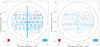 |
Fig. 1 Distribution of all 4530 selected single G-band images on the solar disk in the period from 2006 October 25 to 2013 August 31 (left). Diamonds and squares indicate single G-band images with 2048 × 1024 (3819 images) and 1024 × 1024 (711 images) pixels, respectively. Distribution of all 1013 G-band images (690 images with 2048 × 1024 and 323 images with 1024 × 1024 pixels) with pores on the solar disk (right). The different image sizes are indicated by the filled boxes in the lower left and right corners. The solid line encircles the solar disk, and the dash-dotted line refers to μ = cosθ = 0.6. |
In principle, time-averaged G-band images, which belong to the data set above, are sufficient to derive the morphological and photometric properties of pores. However, including “single” G-band images into the morphological and photometric study, which are not restricted by LCT requirements, significantly broadens the scope and scientific reach of the study. In addition, comparing time-averaged with instantaneous results gives a better understanding of how accurate the measured statistical properties are. Most importantly, now the entire database of Hinode G-band images is at our disposal, which covers more than half a solar cycle.
We restrict our selection of single G-band images to locations on the solar disk, where the center of the FOV is within a circle corresponding to μ = cosθ = 0.6, where θ is the heliocentric angle, i.e., images in close proximity to the solar limb are excluded. On each day, we select one G-band image for each of the observed targets. Targets are considered to be different, if the telescope pointing on the solar disk differ by more than 0.1 μR⊙, where R⊙ is the solar radius. Thus, continuous tracking of an active region over the course of a day can produce two or three images of the same (active) region. The above selection criterion guarantees that images of the same region are spread over time (about 10 h), so that pores will have significantly evolved, thus reducing potential biases.
The single G-band images cover the time period from 2006 October 25 to 2013 August 31, which includes the deep minimum of solar cycle No. 23 and the rise towards the maximum of cycle No. 24. In total 4530 G-band images have been downloaded. However, only 1013 G-band images contain pores, whereas the other images are related to quiet-Sun studies – in particular studies of the center-to-limb variation. The disk coverage of the initial selection of G-band images is indicated in Fig. 1 for both image sizes. Specifically, the 2048 × 1024-pixel images exhibit a peculiar pattern, which consists of two parts: (1) a cross-shaped pattern along the central meridian and the equator, which is typical for center-to-limb variation studies of the quiet Sun and (2) a pattern tracing certain sections of great circles within the solar activity belts. The emergent pattern bears close resemblance to a bright reflection (“the Pope’s revenge”), which appears when the Sun illuminates the stainless steel dome of the Berlin television tower at Alexanderplatz.
This statistical study is based only on a photometric and morphological analysis of G-band images and LCT flow maps, i.e., neither measurements of the magnetic field nor any type of spectroscopic observations are included. In addition, even though most Hinode G-band observations are time-series, we do not include any dynamical aspects related to the evolution of pores. Consequently, the scientific focus is narrower, which however is compensated by a much improved statistical sample of many thousands of solar pores.
3. Feature identification and selection
The identification and selection process of pores follows the same scheme for both single and time-averaged G-band images. Nevertheless, examples discussed in this section are based on pores in single G-band images. A pore is dark feature on the solar surface lacking a penumbra (e.g., Sütterlin et al. 1996). The magnetic field is already sufficiently strong to suppress the convective energy transport. This physical property leads to the first selection criterion: at least one dark core (Icore < 0.6 I0) of at least 10 contiguous pixels must be enclosed by the perimeter of the pore. Additionally, two size thresholds are used to bracket pores: (1) dark features with 125 pixels (0.8 Mm2) or are classified more appropriately as magnetic knots, and (2) dark structures with more than 15625 pixels (100 Mm2) are in all likelihood sunspots, even though there is a substantial overlap in size between sunspots and pores (e.g., Rucklidge et al. 1995).
The criterion that a pore must possess a dark core is very strict and excludes two types of small-scale dark features: (1) darkened patches (intensities down to about 0.8 I0) with a size of one to three granules within the quiet-Sun granulation and (2) roundish dark features (intensities down to about 0.6 I0) with the size of a granule and below within plage regions related to “old” magnetic flux. The first type most likely corresponds likely to azimuth centers (Keppens & Martinez Pillet 1996; Leka & Skumanich 1998; Leka & Steiner 2001), whereas the second coincides with either flux concentrations due to flux pile-up at supergranular boundaries (Keil et al. 1999) or with remnants of decaying pores. This limitation can be alleviated to some extend by correcting instrument stray-light and the telescope’s modulation transfer function (see Mathew et al. 2009). However, the iterative maximum-likelihood deconvolution algorithm is computationally expensive, in particular when many thousands of large-format G-band images are involved. Therefore, we have opted against this type of image correction.
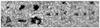 |
Fig. 2 Sample of different types of pores panels a)–g) extracted from the full-sized G-band images. The images are displayed in the range 0.4−1.4 I0. Major tick marks are separated by 2 Mm. The application of a Perona-Malik filter to the G-band image in panel g) is shown in panel h). This filter facilitates the extraction of pores by intensity thresholding. The contours of the pores are marked by solid lines in panel h). Characteristic parameters of the pores are given in Table 2. |
Simple intensity thresholding is too restrictive in determining the boundary of a pore and results in very corrugated boundaries. Perona & Malik (1990) have suggested an approach to detect “semantically meaningful” edges at coarser spatial scales using anisotropic diffusion. While Gaussian smoothing just blurs the image, the Perona-Malik filter conserves the boundaries of an object. We select a conduction coefficient for the anisotropic diffusion equation which favors wider over smaller regions. The property of intra-region smoothing is very powerful in detecting contiguous dark features by thresholding the filtered gray-scale image. Implementing the diffusion process results in an iterative numerical scheme. The process is stopped after 50 iterations, and an intensity threshold of 0.85 I0 is applied to the filtered images identifying features resembling pores (see Fig. 2h). A visual inspection is still required to confirm that the features are actually pores. Various properties of pores can now be computed for all pores from the unfiltered images using the contours of the filtered images as described below. Table 2 summarizes the results for the sample of pores shown in Fig. 2. Processing more than 4500 single G-band images takes about about 1350 min on an Intel Xeon X5460 CPU at 3.16 GHz.
The morphological differences between pores are significant (see Fig. 2). Many pores contain umbral dots (Sobotka et al. 1999) and faint (sometimes even strong) light bridges. Pores can exist in isolation or in proximity to sunspots or other pores. Some pores form chains and even ring-like structures. All these characteristics are not criteria in the visual selection process. The only strong discriminator is the presence of any type of elongated feature resembling penumbral filaments. These are taken as indications that the magnetic field is no longer close to vertical. Furthermore, once a penumbra starts to form, the Evershed flow sets in and the interaction of the magnetic fields with the surrounding plasma has been significantly altered (e.g., Leka & Skumanich 1998; Yang et al. 2003; Langhans et al. 2005). Therefore, any type of filamentary structure within the confines of the identified feature but also in its close proximity results in its exclusion.
In the visual inspection, 438 features are classified as orphan penumbrae, where the filamentary structure dominates the dark cores, 1511 features are sunspots with rudimentary penumbrae, and 68 features are categorized as sunspots because their penumbra encompasses more than half of the sunspot. In 434 cases, features are too close to the boundary of the G-band images and have to be excluded from further analysis. In total, almost 10000 features have been inspected and 7643 pores are kept for further analysis. Yet another 2863 pores have been identified in time-averaged G-band images (Table 1). Thus, to the best of our knowledge, these two data sets comprise the largest sample of pores used in any type of statistical study so far.
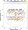 |
Fig. 3 Disk-coverage of all 7643 pores detected in single G-band images. The scale indicates the date when the pores were observed. |
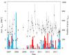 |
Fig. 4 Mean area of pores (“★” symbols) for each month derived from single G-band images. The vertical lines represent 1/5 of the standard deviation of the monthly distributions. The red and blue bars correspond to the number of pores per month (right scale) in the northern and southern hemispheres, respectively. |
The feature identification leads to binary masks containing all pixels belonging to pores. The masks provide easy access to other physical quantities such as the normalized intensity, the position on the solar disk in heliocentric coordinates, and the cosine of the heliocentric angle μ (see Table 2). Standard tools for “blob analysis” (Fanning 2011) are used to derive parameters describing the morphology and the associated flow field of pores. We measure the area covered by pores Apore, the length of the circumference lpore, the mean intensity Imean, the average horizontal flow speed vmean, the divergence ∇ ·v, and the vorticity ∇ × v within pores. The most important ones are the perimeter length (circumference) lpore and area Apore. The connectivity of pixels inside a pore is 4-adjacent, i.e., only horizontal and vertical neighbors are included but not diagonal neighbors. A “chain code” algorithm (Russ 2011) computes the length and area from the perimeter points. The thus calculated area is always smaller than the area represented by the pixels masking the pore. Fitting an ellipse to each pore yields among other parameters the semimajor a and semiminor b axes.
4. Results
The photometric results are based both on single and time-averaged G-band images, whereas the solar cycle dependence is discussed using the former data set, and the analysis of flow fields naturally relies on the latter collection of pores. In the statistical analysis numerical errors are typically small but systematic errors introduced by selection criteria and preconceptions can strongly affect the outcome of a study. Using both single and time-averaged G-band images to measure the photometric and morphological properties of pores provides guidance in interpreting the results and ensures that our conclusions are sound.
4.1. Solar cycle dependence
The distribution of all pores identified on the solar disk in single G-band images is presented in Fig. 3. The color-coded ‘+’ symbols indicate the time and location of the detection. Some pores are situated outside the circle with μ = 0.6 because the FOV covered by the G-band images extends beyond this circle, especially for images with 2048 × 1024 pixels. We observe a pronounced north-south asymmetry during the extended minimum of solar cycle 23 with a larger amount of pores at low latitudes in the southern hemisphere. This trend changes, when most of the pores of the new solar cycle 24 appear at high latitudes in the northern hemisphere. This striking imbalance persists during the rise of solar cycle 24. These observations are in good agreement with photospheric magnetic field measurements at the National Solar Observatory/Kitt Peak (Petrie 2012), in particular with the vector spectro-magnetograph of the Synoptic Optical Long-term Investigations of the Sun (SOLIS, Keller et al. 2003; Henney et al. 2009) instrument suite. In general, the color-coded locations of the pores are an easily perceptible graphic representation of Spörer’s law (see the introduction of Leighton 1969).
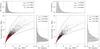 |
Fig. 5 Scatter plots of perimeter length lpore vs. area Apore for single (left) and time-averaged (right) G-band images, which also include the respective frequency distributions. Red symbols “×” mark isolated pores. The lower envelope (solid) of the scatter plots refers to perfectly circular pores (α = 1 in Eqn. 1), while the upper envelope (solid) is given by a scaling factor of α = 2.5. Non-linear least squares fits (dashed) using Eq. (1) lead to scaling factors of α = 1.43 and 1.37 for single and time-averaged G-band images, respectively. Median, mean, and 10th percentile of the frequency distributions (light gray bars) are given by solid, dashed, and dash-dotted lines, respectively. Quantitative values of the measures are specified in the panels for perimeter lengths lpore and areas Apore. Log-normal frequency distributions (solid) properly fit the histograms. |
Figure 4 provides another view of the north-south asymmetry of the pores’ location on the solar disk. The height of the histogram bars corresponds to the number of pores observed in each hemisphere per month. Red and blue colors indicate the northern and southern hemisphere, respectively. Most pores appear in the southern hemisphere during the decline and deep minimum of solar cycle 23. Only in three months, more pores surface in the northern hemisphere. The deep solar minimum also leaves its signature in the pore count. Pores are virtually absent in Hinode G-band images for more than one year (March 2008−April 2009). The dearth of pores ceased at last in early 2010. The north-south asymmetry reversed with the rise of solar cycle 24. However, there are periods (most prominently in 2012 and 2013) when pores are more common in the south. Interestingly, months with a clear hemispheric preference occur more often than months with a balanced pore count. In addition, less pores are detected per month in solar cycle 24 as compared to the previous cycle.
The large number of pores in the sample allows us to search for a potential solar cycle dependence of physical parameters, e.g., the area of the pores. Asterisks in Fig. 4 refer to the average area of the pores for a given month. The standard deviation for each monthly sample is large so that the corresponding vertical bars have to be scaled down by a factor of five. The average area of pores for the entire sample is 4.21 Mm2. The corresponding values for solar cycles 23 and 24 are 4.12 Mm2 and 4.25 Mm2, respectively. There is no obvious trend in area related to the rise or decline of the activity cycle. The sample of pores presented in this study is certainly not complete. This can only be accomplished with synoptic full-disk observations, which are nowadays provided by the Helioseimic and Magnetic Imager (HMI, Scherrer et al. 2012) of the Solar Dynamics Observatory (SDO, Pesnell et al. 2012). However, the reduced spatial resolution of HMI does not permit the detection of small pores.
Scaling factors α and αfit of the square-root dependence between perimeter length lpore and area Apore of a pore.
4.2. Area vs. perimeter
Scatter plots of perimeter length lpore vs. area Apore are depicted for both data sets in Fig. 5. The ratio lpore/Apore is minimal for a perfectly circular pore, i.e., α = 1 in 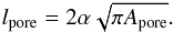 (1)Allperimeter lengths have to be above the curve representing circular objects. We find that the larger the area the farther the points are located from the curve. To quantify this behavior, we compute the scaling factor α with respect to this square-root dependence, which describes both the ellipticity and jaggedness of the pores’ perimeter. The results for various area intervals are presented in Table 3. The overall scaling factor is
  and 1.38 in the interval 0−80 Mm2 for single and time-averaged G-band images, respectively. Notably, the scaling factor increases from α = 1.28 for the smallest pores (0−10 Mm2) to α = 1.85 for larger pores (30−40 Mm2) observed in single G-band images. The trend is the same for time-averaged data, where the scaling factor increases from α = 1.23 for the smallest pores (0−10 Mm2) to α = 1.54 for larger pores (30−40 Mm2). To separate ellipticity from jaggedness, we derive αfit from the semi-major a and -minor b axes of the fitted ellipses (see below) using Ramanjuan’s approximation of the circumference (Villarino 2006). There is a tendency of small pores to have a more circular shape. However, this effect is small compared to the fact that larger pores have more corrugated boundaries. In both data sets only about 20 pores have an area Apore > 40 Mm2, so that they are not listed in Table 3 and are excluded from Fig. 5 for clarity. Lastly, the curve for a scaling factor α = 2.5 is a good upper envelope for the scatter plots.
Figure 5 also contains the frequency distributions of perimeter length lpore and area Apore, which are plotted as gray histogram bars. Their respective parameters are included in each panel. In addition, log-normal distributions have been fitted to the histogram 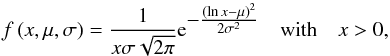 (2)where μ and σ are the mean and standard deviation of the variable x’s (i.e., lpore or Apore) natural logarithm, respectively. The mean μ and standard deviation σ are given in Table 4 along with the moments of the fitted distributions. Mean, median, and 10th percentile are smaller for the fitted distributions because a significant number of pores larger than 4 Mm2 and with perimeter lengths in excess of 10 Mm do not follow the log-normal frequency of occurrence. This relative preponderance of larger pores is also evident in the positive values of the skewness. A possible explanation for this behavior is the tendency of the Perona-Malik filter to join nearby pores. In any case, classifying a chain of pores as either one entity or as separate features is a subjective decision, as long as no other information (e.g., about the magnetic field) enters the decision-making process. Nevertheless, the large kurtosis for the area Apore suggests that most pores are small. More than 77% and 66% of all pores observed in single and time-averaged G-band images, respectively, are smaller than 5 Mm2, i.e., they cover a region of just a few granules. In summary, the overall correspondence between observations and log-normal fits is very good so that Eq. (2) together with Table 4 can serve as a reference for further investigations and theoretical/numerical models of solar pores (e.g., Leka & Steiner 2001; Cameron et al. 2007; Rempel 2011; Hartlep et al. 2012).
Characteristics of the log-normal frequency distributions for area Apore [Mm2] and perimeter length lpore [Mm].
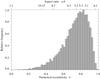 |
Fig. 6 Relative frequency distribution of the numerical eccentricity ε of pores derived from ellipse fitting. The aspect ratio a:b of the semi-major and -minor axes is provided on the upper scale. |
4.3. Eccentricity
The blob-analysis code (Fanning 2011) contains provisions for ellipse fitting (Markwardt 2009) using all pixels within the confines of a pore’s perimeter. Thus, the question can be addressed how circular pores are. This analysis uses only the larger data set based on single G-band images. The numerical eccentricity (Fig. 6) of an ellipse is given by  (3)where e is the linear eccentricity and a and b denote the semi-major and -minor axes, respectively. The aspect ratio of the semi-major and -minor axes a:b is indicated for selected integer ratios, which are sometimes easier to grasp. The mean εmean and median εmed of the numerical eccentricity are 0.74 and 0.76, respectively, which corresponds to an aspect ratio of about 3:2. Less than 7% of all pores have a circular shape with an aspect ratio of less than 8:7, and slightly more than 26% of all pores have aspect ratios lower than 4:3. The tendency of the feature identification algorithm to link some neighboring pores into chains and sometimes even ring-like structure only partially contributes to the trend. In general, smaller pores tend to be more circular as already pointed out when fitting the perimeter length vs. area relationship in Eq. (1).
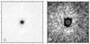 |
Fig. 7 The average of 742 single G-band images containing isolated pores is displayed between a) Imin = 0.54 I0 and Imax = 1.03 I0 and b) in the range (1.00 ± 0.02) I0. The white contour lines correspond to intensities from 0.6–1.0 I0 in increments of 0.1 I0. Major tick marks are separated by 5 Mm. |
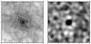 |
Fig. 8 Average velocity a) and divergence b) of 200 isolated pores in time-averaged G-band images. The velocity and divergence are displayed between 0.15–0.5 km s-1 and ± 1 × 10⁻⁴ s-1, respectively. The white contour lines correspond to velocities from 0.15 to 0.3 km s-1 in increments of 0.05 km s-1. Major tick marks are separated by 5 Mm. |
4.4. Prototype of an isolated pore
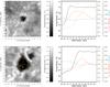 |
Fig. 9 Time-averaged (60-min) G-band images (left) of an isolated pore (top) observed on 2007 February 3 and a residual pore (bottom) observed on 2006 December 7. The arrows indicate magnitude and direction of the horizontal proper motions. Arrow with the length of the grid spacing indicate a speed of 0.5 km s-1. Azimuthally averaged profiles (right) are presented for the time-averaged G-band intensity (solid), the horizontal flow velocities (long-dashed), the divergence (dashed), and the vorticity (dash-dotted). |
Up to now only scalar parameters have been used to describe pores. In the next step, radial intensity profiles are computed, which are representative of a typical pore. Centered on each pore a region-of-interest (ROI) with a size of 20 Mm × 20 Mm is extracted from the G-band images. If the pore is located close to the edge of the images, the ROI is appropriately trimmed. Strong magnetic features in the vicinity of the pore considerably reduce the quiet-Sun intensity. Accordingly, these “dark” regions have to be excluded. Pie-shaped sectors with a width of 1° are centered on the pore. If sectors contain any dark feature, they are left aside when computing the averages. To add a margin of safety, the G-band images are first smoothed by a Gaussian with a FWHM = 1.68 Mm before an intensity threshold of 0.85 I0 is applied to mark contiguous dark regions.
In 742 cases (about 10% of all pores), no other strong magnetic feature is detected at all in the ROI of 20 Mm × 20 Mm. The arithmetic mean of these ROIs is depicted in Fig. 7a scaled between the minimum (Imin = 0.54 I0) and maximum (Imax = 1.03 I0) intensities. The image of the prototypical pore has at first glance a roundish appearance. Only when displayed in a range of ± 2% around the mean quiet-Sun intensity (Fig. 7b) do more details become visible. The outermost contour line referring to I = 1.0 I0 is the only one deviating from a round or oval shape, because even after averaging it inherits some structure from pores of very different shapes (see Fig. 2). It will be interesting to see, if this corrugated boundary is related to the magnetic canopy often observed around pores, which extends well beyond the photometric boundary of the pores (e.g., Keppens & Martinez Pillet 1996; Leka & Steiner 2001; Balthasar & Gömöry 2008). The most striking feature in the average image is the granular pattern of G-band brightenings, which survives the averaging process. These bright features are clearly visible up to about 5 Mm from the prototypical pore’s center, and beyond they still leave an imprint as a faint halo. In conclusion, G-band bright points in proximity to the pores’ boundary are a distinct part of the magnetic flux system.
Using the same criteria as above, we find 200 isolated pores in time-averaged G-band images, which is again about 10% of all pores. The arithmetic mean of the G-band intensity also reveals the signatures of bright points in the surroundings of pores. Average horizontal flow speed and divergence are displayed in Fig. 8. We find low velocity and negative divergence inside pores. The velocity increases monotonously from the center of the prototypical pore to the surrounding granulation. The most conspicuous feature in the divergence map is the ring of positive divergence around the pore. Even after one-hour averaging and computing the arithmetic mean for 200 isolated pores, this ring still survives and asserts the dominance of divergence centers (Roudier et al. 2002) and exploding granules (Vargas Domínguez et al. 2010).
4.5. Flow fields in and around isolated and residual pores
In Fig. 9, two pores out of 2863 pores in the LCT database are presented as an example to explain the data analysis and to introduce the parameters obtained for further study. We compare two pores with different histories and backgrounds: an isolated pore in the vicinity of a sunspot and a residual pore, i.e., the final stage of a decaying sunspot. The isolated pore is located in a supergranular cell within active region NOAA 10940 observed on 2007 February 3 in the neighborhood of a fully developed sunspot, whereas the residual pore is the end product of a satellite sunspot (Verma & Denker 2012) in the vicinity of the highly active and flare-prolific region NOAA 10930 observed on 2006 December 7. We use the time-averaged G-band image as background and superimpose the averaged flow vectors. Both pores are surrounded by a bright intensity ring. However, in case of the residual pore, the bright ring is not regular. An annular structure of positive divergence (not shown) envelops the bright ring like an onion peel. The positive divergence structure contains localized divergence centers, which are related to exploding granules (see Roudier et al. 2002). Pores exhibit inflows in their interior and outflows at their periphery; both are not necessarily symmetric. Around the isolated pore outflows are stronger than inflows.
Parameters describing the morphology of pores and the associated flow field.
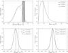 |
Fig. 10 The intensity distribution (top-left) of all pores (solid) can be fitted with two Gaussians, i.e., a dark component with μ1 = 0.62 I0 and σ1 = 0.14 I0 (dashed) and a bright component with μ2 = 0.80 I0 and σ2 = 0.04 I0 (dash-dotted). The gray region outlines the bright component as given by the optimal thresholds T1 = 0.76 I0 and T2 = 0.87 I0. The frequency distributions are also given for the flow speed (top-right), the divergence (bottom-left), and the vorticity (bottom-right) within all pores. The three vertical lines mark the position of the median (solid), mean (long-dashed), and 10th percentile (dash-dotted) of the the speed v, the divergence ∇ ·v, and the vorticity ∇ × v. The divergence and vorticity distributions are fitted with a Gaussian (dashed) having a mean value of μ = −0.14 × 10⁻³ s-1 and −0.01 × 10⁻³ s-1, respectively. |
The parameters describing the morphology for both pores are compiled in Table 5. As expected from a visual inspection, the isolated pore has a smaller eccentricity than the residual pore, i.e., it is more circular. The minimum intensity I is lower in the residual pore. The mean divergence within both pores is negative, indicating converging flows as seen in the superimposed flow vectors. Apart from computing parameters inside pores, we compute radial averages for intensity, velocity, divergence, and vorticity over a radial distance of 6 Mm for all pores. Radial averages are only computed, if pie-shaped segments, which are free of any other dark features, cover at least 180° in azimuth. In the right panel of Fig. 9, the radial averages for both pores have been compiled. For both pores, the intensity is low inside, then monotonically increases, and reaches quiet-Sun levels at the pores’ photometric radius. Just outside the boundary, the intensity reaches a maximum, which corresponds to the bright ring observed around pores in time-averaged G-band images. The divergence changes sign at the boundary, and the location of its maximum is well outside the pores. Interestingly, the divergence maximum extends even beyond the bright circular ring surrounding pores. The high flow speed outside the isolated pore is also evident in the radial averages with the speed reaching values of up to 0.7 km s-1. These two examples befittingly describe the diversity of pores contained in both data sets.
4.6. Frequency distributions
The relative frequency distribution of the G-band intensity for all pores detected in time-averaged G-band images is given in Fig. 10. We compute the mean Imean = 0.65 I0, median Imed = 0.67 I0, and 10th percentile of the frequency distribution I10 = 0.83 I0. The shape of the distribution is characterized by a modal value at higher intensities accompanied by an extended shoulder on the low-intensity side. Interestingly, the frequency distribution increases almost linearly from 0.58 to 0.80 I0. Even though the frequency distribution is not bimodal, we fit two Gaussians to it representing a dark and a bright component. The double-Gaussian fit is justified because dark pores often show bright intrusions, which are most commonly the counterparts of umbral dots, but sometimes features similar to sunspot light bridges are encountered. The respective frequency distribution is given by 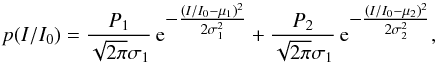 (4)where P1,2 are the probabilities of occurrence with P1 + P2 = 1. Bright features cover about 21.6% of the pores’ area, i.e., P2 = 0.216. Means μ1,2 and standard deviations σ1,2 of the two Gaussians are given in the caption of Fig. 10. Optimal thresholds T1,2 (e.g., Gonzalez & Woods 2002) separate the bright and dark components according to the quadratic equation
 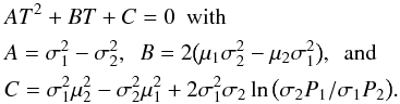 (5)In this case, two thresholds T1 = 0.76 I0 and T2 = 0.87 I0 are required to separate the dark and bright components because of their strong overlap (see gray background in Fig. 10). Combining the two Gaussians results in a bimodal frequency distribution, which is not observed. However, the intensities have been obtained over a wide range of heliocentric angles θ. Both components thus have a distinct CLV in G-band intensity, which affects their means μ1,2(μ = cosθ) and standard deviations σ1,2(μ = cosθ). We have carried out numerical experiments using linear expressions for this functional dependence and successfully recover the general shape of the distribution in Fig. 10. Likewise the disk coverage of all pores is still not sufficient to accurately fit the distinctive frequency distribution at hand. Furthermore, morphological properties and the evolution of pores impact the distribution.
The frequency distribution based on single G-band images is virtually identical to the one shown in Fig. 10. It includes the G-band intensity of about five million pixels belonging to 7643 pores with an equivalent area of more than 32000 Mm2. The mean, median, mode, and 10th percentile of this frequency distribution are Imean = 0.64 I0, Imed = 0.65 I0, Imode = 0.77 I0, and I10 = 0.82 I0, respectively. Again, two Gaussians represent dark (μ1 = 0.60 I0 and σ1 = 0.15 I0) and bright (μ2 = 0.78 I0 and σ2 = 0.055 I0) components. The filling factor of the bright component is about 20% (P2 = 0.19). The two thresholds of T1 = 0.76 I0 and T2 = 0.86 I0 are almost the same as for pores in time-averaged G-band images.
The frequency of occurrence is shown in Fig. 10 for G-band intensity, flow speed, divergence, and vorticity. The distributions include all pixels belonging to pores in time-averaged G-band images. The speed distribution is broad and has a high-velocity tail. The mean speed is low vmean = 0.18 km s-1 inside pores. However, because LCT tracks intensity contrasts, the lack of contrast-rich structures in the dark core potentially leads to lower speeds. The frequency distributions of divergence and vorticity have almost the same shape. We fit the divergence distribution with a Gaussian 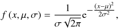 (6)with a standard deviation of σ = 0.11 × 10⁻³ s-1 and a mean of μ = −0.14 × 10⁻³ s-1. The negative mean value of the divergence inside pores indicates inflows, which we also see in the two pores presented as examples in Fig. 9. A normal distribution is likewise a valid representation of the vorticity with a mean close to zero and a standard deviation of σ = 0.10 × 10⁻³ s-1. This probably indicates that on average neither twisting nor spiraling motion are present inside pores.
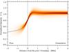 |
Fig. 11 Typical intensity profile of a pore based on single G-band images after azimuthal averaging. The vertical dash-dotted line indicates the boundary of the pore corresponding to the intensity threshold of 0.85 I0. The background image shows the two-dimensional frequency distribution of the intensities. |
4.7. Radial averages
To express the average properties of intensity and flow fields around pores in more quantitative terms, we compute for each instance azimuthal averages of intensity, velocity, divergence, and radial component of velocity. Pores come in a variety of shapes so that computing meaningful azimuthal averages becomes a challenging task. In the following, we describe two different approaches to compute azimuthal averages based on single and time-averaged G-band images.
Morphological dilation/erosion using disk-shaped binary masks of increasing/decreasing size is one option to tackle this problem as demonstrated for single G-band images (see Fig. 11). These operations are applied to binary masks outlining each pore such that they either expand or shrink the region. Subtracting a region from the next smaller one results in a ring-like mask, which still preserves the shape of the pore. The ring-like structure becomes more circular for larger distances from the pore’s origin, which is a desired feature for an azimuthal average. Taking the mean of the positions and intensities along the circular ring of pixels yields a radial intensity profile, which is resampled to a regular grid. This allows us not only to compute a global mean of all intensity profiles but also to derive the intensity distribution at each radial position.
Distances are measured from the prototypical pore’s edge in Fig. 11. We find a preponderance of G-band brightenings in proximity (about 0.64 Mm) to the pore’s boundary (vertical dash-dotted line). G-band bright points are located well within the ring-like structure of divergence centers (e.g., Roudier et al. 2002) at a distance of about 3.5 Mm from the pore’s boundary. Sobotka et al. (1999) relate recurring G-band bright points in the vicinity of pores to mesogranular flows (November & Simon 1988). The intensity gradient is dI/dr ≈ 0.7 I0 Mm-1 in the linear part of the radial intensity profile. Using the edge of the pore as point of reference has the advantage of describing the intensity inside a pore regardless of its size. The frequency distribution first flares out and then tapers off, because pores with radii larger than 1 Mm are rare. The tendency that larger pores are darker (e.g., Keppens & Martinez Pillet 1996) is evident but the interior gradient dI/dr ≈ 0.06 I0 Mm-1 is shallow. The narrowing of the frequency distribution at the edge of the pore is an artifact of the intensity thresholding of the Perona-Malik filtered images. That the radial intensity profile does not reach unity for large distances from the pore is because of the asymmetric frequency distribution with an extended tail towards higher intensities and the faint halo of G-band brightenings seen in Fig. 7b.
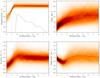 |
Fig. 12 Azimuthally averaged profiles for intensity (top-left), flow velocity (top-right), divergence (bottom-left), and radial velocity (bottom-right) for all pores. The profiles are computed for normalized radial distances, where r/Rpore = 0 and r/Rpore = 1 indicate the center and the boundary of the pores, respectively. The frequency of occurrence is shown as a shaded background, where darker regions refer to more commonly encountered values. In the intensity profile (top-left), the solid curve represents the percentage of increase in average intensity, and the dashed line reflects our choice of the intensity threshold (0.85 I0) delimiting pores. The white line corresponds to an intensity gradient of |
An alternate approach has been employed to compute azimuthal averages for pores contained in time-averaged G-band images. Starting with more than 2863 pores we deselect pores, which are at FOV’s border, as their radial averages rely on a much smaller number of points. Thus, we are left with 2300 pores. The averages are computed for a FOV of 300 × 300 pixels (24 Mm × 24 Mm) centered on the pores’ origin. Pores are not always circular. Hence, considering their irregular shapes while computing azimuthally average profiles outside and inside pores, we grow/shrink the region successively by 100/50 pixels using morphological dilation/erosion. Shrinking of a region is stopped, once the origin is reached. In addition, we exclude any 1°-wide sector that contains either dark pores or any other dark feature. To facilitate the comparison of all pore profiles, we interpolate individual profiles on a regular grid of normalized radius RN = r/Rpore. These averaged profiles are depicted in Fig. 12. We also compute frequency distributions at each normalized radial position for every physical parameter. The distributions are included in the panels as shaded backgrounds, where darker gradations of color represent a larger frequency of occurrence.
In the averaged intensity profile, the intensity is low inside the prototypical pore and slowly approaches a level slightly larger than I/I0 = 1. The spread in intensity values (shaded background) is small and the mode conforms more closely to I/I0 = 1. The intensity has a gradient of  in the linear part of the radial intensity profile as indicated by a white-line in Fig. 12. The intensity peak, which we see in the azimuthal profile of two pores (Fig. 9), is much harder to discern in the averaged intensity profile. To clearly identify the peak in intensity, we also plot the excess brightness with respect to the mean intensity at the FOV’s periphery. These values were multiplied by a factor of hundred. Thus, the scale in Fig. 12 can be interpreted as the excess brightness in percent. As evident from the plot, there is an increase of about 0.7% in intensity around the border of pores (at about 2 RN) indicating that on average pores are surrounded by many G-band bright points. Despite using two different approaches, the overall appearance of the azimuthally averaged intensity profiles is virtually the same, which confirms that both approaches are effective in deducing the physical properties of pores.
The average velocity profile does not show any peculiarities. Inside the prototypical pore the velocities are low, then they monotonically increase until reaching quiet-Sun values. However, the velocity distributions as a function of normalized radius are narrower out to about three times the pore’s radius. We attribute this compactness and the lower mean flow speed to the presence of a magnetic canopy around pores (e.g., Sütterlin et al. 1996), which inhibits to some extend the horizontal plasma flows. The mean velocity outside the pore RN ≫ 1 is about 0.31 km s-1. The median is 0.32 km s-1 and the 10th percentile amounts to 0.33 km s-1. To gain more insight how the flow speed varies around pores, we compute the radial component of horizontal flow velocity using vrad = vxcosθ + vysinθ, where θ is the azimuth angle measured counterclockwise from the positive x-axis around the center of the pores. The radial velocity starts close to zero (−0.01 km s-1) inside the pore, then decreases to reach a minimum of −0.12 km s-1 at around RN = 1.1, before increasing again attaining positive values at RN = 2.6. Finally, it approaches its maximum (0.05 km s-1) at around RN = 4.6 before leveling out to zero far away from the pore’s origin. The width of the frequency distributions is largest near RN = 4.
The divergence is negative inside the pore and switches to positive values at around RN = 1.6 before attaining a maximum of 0.05 × 10⁻³ s-1 at RN = 2.3. Once the maximum is reached, the divergence slowly converges on zero. The divergence peak at around RN = 2.3 is also clearly visible in the width of the frequency distribution. This divergence peak has already been discussed in Sect. 4.5 in the context of the isolated and residual pores. A negative divergence indicates inflows inside pores and positive values surrounding pores suggest outward motions near the borders. The zero crossing is located at RN = 4.
To summarize our findings, we compile all radially averaged profiles in Fig. 13 to furnish a complete picture of the photometric and flow characteristics around a prototypical pore. We have chosen an intensity threshold of 0.85 I0 to identify pores, and all the results discussed so far refer to this choice. Now, the question arises why not use an intensity threshold of 1.0 I0 for the boundary of a pore. The contrast between bright granules and dark intergranular lanes in G-band images renders such an approach futile leading to ill-defined boundaries for individual pores. Only after averaging over many pores and taking an azimuthal average can, a ‘photometric radius’ of about 1.4 RN be determined when approaching the mean quiet-Sun intensity. This is about 40% larger than our original definition of a pore’s boundary. Hence, all linear dimensions have to be scaled by 40% when referring to the photometric radius.
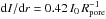
 |
Fig. 13 Azimuthally averaged profiles of intensity (solid), flow velocity (long-dashed), divergence (dashed), and radial velocity (dash-dotted) for all pores (same as Fig. 11 using a similar layout to the one in Fig. 8). Two dashed lines represent our choice of intensity threshold (0.85 I0) and the photometric radius of pores (1.0 I0). The solid line in the center is provided as a visual guide for the zero-crossing of divergence and radial velocity. The short colored vertical lines mark the extreme values and zero-crossings. These markers are replicated on the abscissa to assist in finding the corresponding normalized radii. |
Moving outwards from pore’s border, we find an intensity peak around RN = 2.1, which is the average location of the encircling G-bands bright points. Inspecting the horizontal flows, as expected, the radial component of the horizontal velocity vrad is zero at the center of the pore. The strongest inflows, i.e., the minimum of vrad is observed at the location RN = 1.1, which is virtually identical to our choice of the pore’s boundary (intensity threshold of 0.85 I0). The radial velocity changes sign at RN = 2.6 slightly outside the intensity maximum (ring of G-band brightenings), which indicates that horizontal inflows start well outside the pore’s border. The radial flow field of pores reaches significantly outward with a maximum of vrad at RN = 4.6 before approaching zero at a spatial scale corresponding to the supergranular cell size. To identify sources and sinks of the flow fields in the vicinity of pores, we compute the divergence ∇·v. The divergence is zero at RN = 1.6, which corresponds to the photometric radius RN = 1.4. Hence, we can define the photometric radius also as the location, where the divergence ∇·v = 0. The maximum of the divergence is located between the maxima of intensity and radial velocity, which represent two rings encircling pores like an onion skin (e.g., Sobotka et al. 1999; Roudier et al. 2002). However, the in- and outflows in pores are easier to grasp employing the radial component of the horizontal velocity. The divergence has contributions from both radial and tangential velocity components, whereas vrad is just the velocity vector projected onto the unit vector in the radial direction.
5. Conclusions
Pores represent two stages in the evolution of sunspots, either as a dark umbral core forming a penumbra when growing to become a sunspot or as a decaying sunspot loosing its penumbra. Many pores, however, never reach this transient period. Regardless of the pores’ evolutionary phase, their general statistical properties still improve our understanding of how sunspots form and decay.
All previous statistical studies of pores have been campaign-driven and have not been designed as systematic surveys. We present the first comprehensive statistical study of pores concerning their morphology, photometric properties, and associated horizontal flow fields. This survey makes use of the extensive database of the Japanese Hinode mission. We have tried to minimize potential biases, but we have to admit that the study is certainly not bias-free. The target selection based on “Hinode Observing Programs” favors flare-prolific active regions, i.e., sunspot groups with complex magnetic field configurations and (multiple) tangled magnetic neutral lines. On the other hand, a large number of Hinode quiet-Sun observations is void of any pores indicating that isolated pores are surprisingly rare. They only amount to about 10% of the pores in the sample.
The newly created LCT database (Verma & Denker 2011) facilitates statistical studies of flows around solar features in a straightforward manner. In total, 7643/2863 pores (single/time-averaged G-band images) contribute to the current analysis. We have computed perimeters and areas describing the morphology of pores, and we provide the radial averages for intensity, velocity, divergence, and radial component of the horizontal velocity. Two pores have been presented as an example to illustrate the data analysis strategy and the types of parameters available for further examination. Despite its broad scope, the statistical investigation of pores has not yet reached its culmination. Other physical parameters, most importantly the magnetic field and Doppler velocities, and the temporal evolution of pores have to be included. In principle, this can be accomplished by using synoptic SDO data with excellent coverage but at the moment, such work has to be deferred until a future time.
In summary, we recite the most important findings based on morphology, photometric properties, and horizontal proper motions:
-
(1)
A pronounced north-south asymmetry is observed in thedistribution of pores on the solar disk (Fig. 3).During the extended minimum of solar cycle 23, porespredominantly appear at low latitudes in the southernhemisphere. However, this trend changes with the rise of the newsolar cycle 24, when pores are more commonly encountered athigh latitudes in the northern hemisphere (Fig. 4).
-
(2)
In general pores are not circular. Ellipse fitting (Fig. 6) yields a typical aspect ratio of 3:2 between semi-major and minor axes. Only 7% of all pores identified in single G-band images have a close-to-circular shape with an aspect ratio smaller than 8:7.
-
(3)
Most pores are small. About 75%/66% (single/time-averaged G-band images) of all pores are smaller than 5 Mm2 (Fig. 5), which is comparable to an area covered by just a few granules. Interestingly, smaller pores tend to be more circular and have less corrugated boundaries. This is partially explained by the tendency of larger pores to align in chains and sometimes even in ring-like structures. The feature identification algorithm does not always separate elongated features into their constituent parts.
-
(4)
Averaging all 742 isolated pores detected in single G-band images results in, at least at first glance, a roundish prototypical pore. Only after narrowing the contrast range to ±2% around quiet-Sun intensity, does this representative pore exhibits a corrugated boundary surrounded by a bright, granular intensity distribution brought about by averaging a multitude of G-band brightenings. Thus, G-band bright points encircling pores constitute a distinct part of the magnetic flux system. Furthermore, contours of the pore close to quiet-Sun intensity levels are oval with the longer axis in the north-south direction. It is tempting to relate the distinct east-west asymmetry of the bright halo depicted in Fig. 7 to that of the moat around sunspots (Sobotka & Roudier 2007). However, this lopsidedness is neither found in intensity nor in the velocity and divergence maps (Fig. 8) of the representative pore based on time-averaged G-band images.
-
(5)
The intensity distribution of the pores’ interior has a distinct shape (top-left panel of Fig. 10), which can be reproduced by two Gaussians representing dark and bright components. A double peak is absent because both mean and width of the Gaussians depend on the heliocentric angle θ. This dependency is expected to be stronger for bright features (umbral dots and light bridges), if the CLV of G-band bright-points is taken as a guide.
-
(6)
The averaged, radial intensity profiles of 7643/2863 pores show a distinct peak (Fig. 11 and top-left panel of Fig. 12), which comes out more clearly in radial profiles of individual pores. This peak indicates the presence of bright features encircling pores. Because the origin of G-band bright points is related to the physics of small-scale flux tubes (e.g., Steiner et al. 2001; Schüssler et al. 2003), it would be hasty to conclude that the bright ring is due to the convective energy blocked by the strong magnetic fields inside the pore.
-
(7)
The frequency distributions of divergence and vorticity within pores are easily fitted with Gaussian frequency distributions (bottom panels in Fig. 10). The divergence is predominantly negative within pores strongly suggesting inflows. The mean value of the vorticity is about zero in the pores’ interior pointing to the absence of twisted or spiraling motions.
-
(8)
The radial component of horizontal velocities is negative inside the prototypical pore and approaches positive values outside the pore (Fig. 13). The negative values inside imply inflows inside while outflows start about two radii from the pore’s center.
-
(9)
Inflows and outflows seen in the radial velocity profile can also be traced in the divergence profile. The maximum of the radial divergence radial profile matches the zero-crossing of the radial velocity profile (Fig. 13). The ring of positive divergence encircling pores corresponds to the location of exploding granules (Keil et al. 1999; Roudier et al. 2002; Vargas Domínguez et al. 2010).
-
(10)
The photometric radius of the prototypical pore is the location where the pore’s intensity profile reaches quiet-Sun values (Fig. 13). This radius is inherently larger than the one based on the intensity threshold used in identifying pores. The photometric radius roughly corresponds to the location, where the radial velocity has a minimum (strongest outflow) and the the divergence is zero.
There is an ongoing discussion regarding in- and outflows around pores. Many studies (e.g., Roudier et al. 2002; Vargas Domínguez et al. 2010) find outflows outside and inflows inside pores. In our study, we present the exact location, where the in- and outflows (on average) start and terminate. However, to contribute to the debate about the existence of moat and Evershed flow around pores (e.g., Vargas Domínguez et al. 2008), we need more information. Hence, the next step is to carry out a similar study for Doppler velocities and magnetic fields. Current simulations of magnetic features such as pores usually describe individual pores (e.g., Leka & Steiner 2001; Cameron et al. 2007; Rempel & Schlichenmaier 2011). It will be very instructive, once future modeling efforts produce ensembles of pores for different input parameters and in different magnetic settings. In principle, these modeled pores should reproduce the mean values together with the shape of the specific distributions for all physical parameters, presented in this statistical study.
The results of this ongoing research are only a first step towards a better understanding of pores and provide important information for numerical models (Leka & Steiner 2001; Cameron et al. 2007; Rempel 2011). Moving forward, SDO/HMI data offer another opportunity to study the solar cycle dependence and temporal evolution of pores. Even though the spatial resolution is much reduced as compared to Hinode/SOT, quasi-simultaneous intensity maps, magnetograms, and dopplergrams cover a much broader parameter space, thus providing even tighter boundary conditions for theoretical models. Images taken in the extreme ultraviolet are an addtional resource provided by SDO, which potentially links the photospheric properties of pores to the dynamics of the Sun’s upper atmosphere.
Acknowledgments
Hinode is a Japanese mission developed and launched by ISAS/JAXA, collaborating with NAOJ as a domestic partner, NASA and STFC (UK) as international partners. Scientific operation of the Hinode mission is conducted by the Hinode science team organized at ISAS/JAXA. This team mainly consists of scientists from institutes in the partner countries. Support for the post-launch operation is provided by JAXA and NAOJ (Japan), STFC (UK), NASA, ESA, and NSC (Norway). MV expresses her gratitude for the generous financial support by the German Academic Exchange Service (DAAD) in the form of a PhD scholarship. CD was supported by grant DE 787/3-1 of the German Science Foundation (DFG). We would like to thank Drs. Nazaret Bello González, Karin Muglach, Horst Balthasar, and Christoph Kuckein for carefully reading the manuscript and providing ideas, which significantly enhanced the paper.
References
- Balthasar, H., & Gömöry, P. 2008, A&A, 488, 1085 [NASA ADS] [CrossRef] [EDP Sciences] [Google Scholar]
- Balthasar, H., Collados, M., & Muglach, K. 2000, Astron. Nachr., 321, 121 [NASA ADS] [CrossRef] [Google Scholar]
- Bray, R. J., & Loughhead, R. E. 1964, Sunspots (London: The International Astrophysics Series, Chapman & Hall) [Google Scholar]
- Cabrera Solana, D., Bellot Rubio, L. R., Beck, C., & del Toro Iniesta, J. C. 2006, ApJL, 649, L41 [NASA ADS] [CrossRef] [Google Scholar]
- Cameron, R., Schüssler, M., Vögler, A., & Zakharov, V. 2007, A&A, 474, 261 [NASA ADS] [CrossRef] [EDP Sciences] [Google Scholar]
- Deng, N., Choudhary, D. P., Tritschler, A., et al. 2007, ApJ, 671, 1013 [NASA ADS] [CrossRef] [Google Scholar]
- Denker, C. 1998, Sol. Phys., 180, 81 [NASA ADS] [CrossRef] [Google Scholar]
- Fanning, D. W. 2011, Coyote’s Guide to Traditional IDL Graphics (Fort Collins, Colorado: Coyote Book Publishing) [Google Scholar]
- Gonzalez, R. C., & Woods, R. E. 2002, Digital Image Processing (Upper Saddle River, New Jersey: Prentice-Hall) [Google Scholar]
- Hartlep, T., Busse, F. H., Hurlburt, N. E., & Kosovichev, A. G. 2012, 419, 2325 [Google Scholar]
- Henney, C. J., Keller, C. U., Harvey, J. W., et al. 2009, in Solar Polarization V, eds. S. V. Berdyugina, K. N. Nagendra, & R. Ramelli, ASP Conf. Ser., 405, 47 [Google Scholar]
- Hirzberger, J. 2003, A&A, 405, 331 [NASA ADS] [CrossRef] [EDP Sciences] [Google Scholar]
- Keil, S. L., Balasubramaniam, K. S., Smaldone, L. A., & Reger, B. 1999, ApJ, 510, 422 [NASA ADS] [CrossRef] [Google Scholar]
- Keller, C. U., Harvey, J. W., & Giampapa, M. S. 2003, in Innovative Telescopes and Instrumentation for Solar Astrophysics, eds. S. L. Keil, & S. V. Avakyan, Proc. SPIE, 4853, 194 [Google Scholar]
- Keppens, R., & Martinez Pillet, V. 1996, A&A, 316, 229 [NASA ADS] [Google Scholar]
- Kosugi, T., Matsuzaki, K., Sakao, T., et al. 2007, Sol. Phys., 243, 3 [NASA ADS] [CrossRef] [Google Scholar]
- Langhans, K., Scharmer, G. B., Kiselman, D., Löfdahl, M. G., & Berger, T. E. 2005, A&A, 436, 1087 [NASA ADS] [CrossRef] [EDP Sciences] [Google Scholar]
- Leighton, R. B. 1969, ApJ, 156, 1 [Google Scholar]
- Leka, K. D., & Skumanich, A. 1998, ApJ, 507, 454 [NASA ADS] [CrossRef] [Google Scholar]
- Leka, K. D., & Steiner, O. 2001, ApJ, 552, 354 [NASA ADS] [CrossRef] [Google Scholar]
- Markwardt, C. B. 2009, in Astronomical Data Analysis Software and Systems XVIII, eds. D. A. Bohlender, D. Durand, & P. Dowler, ASP Conf. Ser., 411, 251 [Google Scholar]
- Mathew, S. K., Zakharov, V., & Solanki, S. K. 2009, A&A, 501, L19 [NASA ADS] [CrossRef] [EDP Sciences] [Google Scholar]
- Montesinos, B., & Thomas, J. H. 1997, Nature, 390, 485 [NASA ADS] [CrossRef] [Google Scholar]
- November, L. J., & Simon, G. W. 1988, ApJ, 333, 427 [Google Scholar]
- Perona, P., & Malik, J. 1990, IEEE Trans. Pattern Anal. Mach. Intell., 12, 629 [CrossRef] [Google Scholar]
- Pesnell, W. D., Thompson, B. J., & Chamberlin, P. C. 2012, Sol. Phys., 275, 3 [NASA ADS] [CrossRef] [Google Scholar]
- Petrie, G. J. D. 2012, Sol. Phys., 281, 577 [NASA ADS] [CrossRef] [Google Scholar]
- Rempel, M. 2011, ApJ, 740, 15 [NASA ADS] [CrossRef] [Google Scholar]
- Rempel, M., & Schlichenmaier, R. 2011, Liv. Rev. Space Phys., 8, 3 [Google Scholar]
- Roudier, T., Bonet, J. A., & Sobotka, M. 2002, A&A, 395, 249 [NASA ADS] [CrossRef] [EDP Sciences] [Google Scholar]
- Rucklidge, A. M., Schmidt, H. U., & Weiss, N. O. 1995, 273, 491 [Google Scholar]
- Russ, J. C. 2011, The Image Processing Handbook (Boca Raton, Florida: CRC Press) [Google Scholar]
- Sainz Dalda, A., Vargas Domínguez, S., & Tarbell, T. D. 2012, ApJ, 746, L13 [NASA ADS] [CrossRef] [Google Scholar]
- Sankarasubramanian, K., & Rimmele, T. 2003, ApJ, 598, 689 [NASA ADS] [CrossRef] [Google Scholar]
- Scherrer, P. H., Schou, J., Bush, R. I., et al. 2012, Sol. Phys., 275, 207 [Google Scholar]
- Schüssler, M., Shelyag, S., Berdyugina, S., Vögler, A., & Solanki, S. K. 2003, ApJ, 597, L173 [NASA ADS] [CrossRef] [Google Scholar]
- Sobotka, M., & Roudier, T. 2007, A&A, 472, 277 [NASA ADS] [CrossRef] [EDP Sciences] [Google Scholar]
- Sobotka, M., Brandt, P. N., & Simon, G. W. 1999, A&A, 348, 621 [NASA ADS] [Google Scholar]
- Steiner, O., Hauschildt, P. H., & Bruls, J. 2001, A&A, 372, L13 [NASA ADS] [CrossRef] [EDP Sciences] [Google Scholar]
- Sütterlin, P. 1998, A&A, 333, 305 [NASA ADS] [Google Scholar]
- Sütterlin, P., & Wiehr, E. 1998, A&A, 336, 367 [NASA ADS] [Google Scholar]
- Sütterlin, P., Schröter, E. H., & Muglach, K. 1996, SoPh, 164, 311 [Google Scholar]
- Thomas, J. H., & Montesinos, B. 1993, ApJ, 407, 398 [NASA ADS] [CrossRef] [Google Scholar]
- Tildesley, M. J., & Weiss, N. O. 2004, 350, 657 [Google Scholar]
- Tsuneta, S., Ichimoto, K., Katsukawa, Y., et al. 2008, Sol. Phys., 249, 167 [NASA ADS] [CrossRef] [Google Scholar]
- Uitenbroek, H., Balasubramaniam, K. S., & Tritschler, A. 2006, ApJ, 645, 776 [NASA ADS] [CrossRef] [Google Scholar]
- Vargas Domínguez, S., Rouppe van der Voort, L., Bonet, J. A., et al. 2008, ApJ, 679, 900 [NASA ADS] [CrossRef] [Google Scholar]
- Vargas Domínguez, S., de Vicente, A., Bonet, J. A., & Martínez Pillet, V. 2010, A&A, 516, A91 [NASA ADS] [CrossRef] [EDP Sciences] [Google Scholar]
- Verma, M., & Denker, C. 2011, A&A, 529, A153 [NASA ADS] [CrossRef] [EDP Sciences] [Google Scholar]
- Verma, M., & Denker, C. 2012, A&A, 545, A92 [NASA ADS] [CrossRef] [EDP Sciences] [Google Scholar]
- Verma, M., Balthasar, H., Deng, N., et al. 2012, A&A, 538, A109 [NASA ADS] [CrossRef] [EDP Sciences] [Google Scholar]
- Verma, M., Steffen, M., & Denker, C. 2013, A&A, 555, A136 [NASA ADS] [CrossRef] [EDP Sciences] [Google Scholar]
- Villarino, M. B. 2006, J. Ineq. Pure Appl. Math., 7, 21 [Google Scholar]
- Wang, H., & Zirin, H. 1992, Sol. Phys., 140, 41 [NASA ADS] [CrossRef] [Google Scholar]
- Yang, G., Xu, Y., Wang, H., & Denker, C. 2003, ApJ, 597, 1190 [NASA ADS] [CrossRef] [Google Scholar]
- Zuccarello, F., Romano, P., Guglielmino, S. L., et al. 2009, A&A, 500, L5 [NASA ADS] [CrossRef] [EDP Sciences] [Google Scholar]
All Tables
Scaling factors α and αfit of the square-root dependence between perimeter length lpore and area Apore of a pore.
Characteristics of the log-normal frequency distributions for area Apore [Mm2] and perimeter length lpore [Mm].
All Figures
|
Fig. 1 Distribution of all 4530 selected single G-band images on the solar disk in the period from 2006 October 25 to 2013 August 31 (left). Diamonds and squares indicate single G-band images with 2048 × 1024 (3819 images) and 1024 × 1024 (711 images) pixels, respectively. Distribution of all 1013 G-band images (690 images with 2048 × 1024 and 323 images with 1024 × 1024 pixels) with pores on the solar disk (right). The different image sizes are indicated by the filled boxes in the lower left and right corners. The solid line encircles the solar disk, and the dash-dotted line refers to μ = cosθ = 0.6. |
| In the text | |
|
Fig. 2 Sample of different types of pores panels a)–g) extracted from the full-sized G-band images. The images are displayed in the range 0.4−1.4 I0. Major tick marks are separated by 2 Mm. The application of a Perona-Malik filter to the G-band image in panel g) is shown in panel h). This filter facilitates the extraction of pores by intensity thresholding. The contours of the pores are marked by solid lines in panel h). Characteristic parameters of the pores are given in Table 2. |
| In the text | |
|
Fig. 3 Disk-coverage of all 7643 pores detected in single G-band images. The scale indicates the date when the pores were observed. |
| In the text | |
|
Fig. 4 Mean area of pores (“★” symbols) for each month derived from single G-band images. The vertical lines represent 1/5 of the standard deviation of the monthly distributions. The red and blue bars correspond to the number of pores per month (right scale) in the northern and southern hemispheres, respectively. |
| In the text | |
|
Fig. 5 Scatter plots of perimeter length lpore vs. area Apore for single (left) and time-averaged (right) G-band images, which also include the respective frequency distributions. Red symbols “×” mark isolated pores. The lower envelope (solid) of the scatter plots refers to perfectly circular pores (α = 1 in Eqn. 1), while the upper envelope (solid) is given by a scaling factor of α = 2.5. Non-linear least squares fits (dashed) using Eq. (1) lead to scaling factors of α = 1.43 and 1.37 for single and time-averaged G-band images, respectively. Median, mean, and 10th percentile of the frequency distributions (light gray bars) are given by solid, dashed, and dash-dotted lines, respectively. Quantitative values of the measures are specified in the panels for perimeter lengths lpore and areas Apore. Log-normal frequency distributions (solid) properly fit the histograms. |
| In the text | |
|
Fig. 6 Relative frequency distribution of the numerical eccentricity ε of pores derived from ellipse fitting. The aspect ratio a:b of the semi-major and -minor axes is provided on the upper scale. |
| In the text | |
|
Fig. 7 The average of 742 single G-band images containing isolated pores is displayed between a) Imin = 0.54 I0 and Imax = 1.03 I0 and b) in the range (1.00 ± 0.02) I0. The white contour lines correspond to intensities from 0.6–1.0 I0 in increments of 0.1 I0. Major tick marks are separated by 5 Mm. |
| In the text | |
|
Fig. 8 Average velocity a) and divergence b) of 200 isolated pores in time-averaged G-band images. The velocity and divergence are displayed between 0.15–0.5 km s-1 and ± 1 × 10⁻⁴ s-1, respectively. The white contour lines correspond to velocities from 0.15 to 0.3 km s-1 in increments of 0.05 km s-1. Major tick marks are separated by 5 Mm. |
| In the text | |
|
Fig. 9 Time-averaged (60-min) G-band images (left) of an isolated pore (top) observed on 2007 February 3 and a residual pore (bottom) observed on 2006 December 7. The arrows indicate magnitude and direction of the horizontal proper motions. Arrow with the length of the grid spacing indicate a speed of 0.5 km s-1. Azimuthally averaged profiles (right) are presented for the time-averaged G-band intensity (solid), the horizontal flow velocities (long-dashed), the divergence (dashed), and the vorticity (dash-dotted). |
| In the text | |
|
Fig. 10 The intensity distribution (top-left) of all pores (solid) can be fitted with two Gaussians, i.e., a dark component with μ1 = 0.62 I0 and σ1 = 0.14 I0 (dashed) and a bright component with μ2 = 0.80 I0 and σ2 = 0.04 I0 (dash-dotted). The gray region outlines the bright component as given by the optimal thresholds T1 = 0.76 I0 and T2 = 0.87 I0. The frequency distributions are also given for the flow speed (top-right), the divergence (bottom-left), and the vorticity (bottom-right) within all pores. The three vertical lines mark the position of the median (solid), mean (long-dashed), and 10th percentile (dash-dotted) of the the speed v, the divergence ∇ ·v, and the vorticity ∇ × v. The divergence and vorticity distributions are fitted with a Gaussian (dashed) having a mean value of μ = −0.14 × 10⁻³ s-1 and −0.01 × 10⁻³ s-1, respectively. |
| In the text | |
|
Fig. 11 Typical intensity profile of a pore based on single G-band images after azimuthal averaging. The vertical dash-dotted line indicates the boundary of the pore corresponding to the intensity threshold of 0.85 I0. The background image shows the two-dimensional frequency distribution of the intensities. |
| In the text | |
|
Fig. 12 Azimuthally averaged profiles for intensity (top-left), flow velocity (top-right), divergence (bottom-left), and radial velocity (bottom-right) for all pores. The profiles are computed for normalized radial distances, where r/Rpore = 0 and r/Rpore = 1 indicate the center and the boundary of the pores, respectively. The frequency of occurrence is shown as a shaded background, where darker regions refer to more commonly encountered values. In the intensity profile (top-left), the solid curve represents the percentage of increase in average intensity, and the dashed line reflects our choice of the intensity threshold (0.85 I0) delimiting pores. The white line corresponds to an intensity gradient of |
| In the text | |
|
Fig. 13 Azimuthally averaged profiles of intensity (solid), flow velocity (long-dashed), divergence (dashed), and radial velocity (dash-dotted) for all pores (same as Fig. 11 using a similar layout to the one in Fig. 8). Two dashed lines represent our choice of intensity threshold (0.85 I0) and the photometric radius of pores (1.0 I0). The solid line in the center is provided as a visual guide for the zero-crossing of divergence and radial velocity. The short colored vertical lines mark the extreme values and zero-crossings. These markers are replicated on the abscissa to assist in finding the corresponding normalized radii. |
| In the text | |
Current usage metrics show cumulative count of Article Views (full-text article views including HTML views, PDF and ePub downloads, according to the available data) and Abstracts Views on Vision4Press platform.
Data correspond to usage on the plateform after 2015. The current usage metrics is available 48-96 hours after online publication and is updated daily on week days.
Initial download of the metrics may take a while.