| Issue |
A&A
Volume 556, August 2013
|
|
|---|---|---|
| Article Number | A104 | |
| Number of page(s) | 12 | |
| Section | The Sun | |
| DOI | https://doi.org/10.1051/0004-6361/201321826 | |
| Published online | 05 August 2013 | |
Structure of solar coronal loops: from miniature to large-scale ⋆
1 Max-Planck Institute for Solar System Research, 37191 Katlenburg-Lindau, Germany
e-mail: peter@mps.mpg.de
2 Heliophysics Division, NASA Goddard Space Flight Center, Greenbelt, MD 20771, USA
3 Southwest Research Institute, Instrumentation and Space Research Division, Boulder, CO 80302, USA
4 Marshall Space Flight Center, NASA, Mail Code ZP13, MSFC, Alabama 35812, USA
5 Harvard-Smithsonian Center for Astrophysics, 60 Garden Street, Cambridge, Massachusetts 01238, USA
6 Center for Space and Aeronautic Research, University of Alabama, Huntsville, Alabama 35812, USA
Received: 3 May 2013
Accepted: 20 June 2013
Aims. We use new data from the High-resolution Coronal Imager (Hi-C) with its unprecedented spatial resolution of the solar corona to investigate the structure of coronal loops down to 0.2′′.
Methods. During a rocket flight, Hi-C provided images of the solar corona in a wavelength band around 193 Å that is dominated by emission from Fe xii showing plasma at temperatures around 1.5 MK. We analyze part of the Hi-C field-of-view to study the smallest coronal loops observed so far and search for the possible substructuring of larger loops.
Results. We find tiny 1.5 MK loop-like structures that we interpret as miniature coronal loops. Their coronal segments above the chromosphere have a length of only about 1 Mm and a thickness of less than 200 km. They could be interpreted as the coronal signature of small flux tubes breaking through the photosphere with a footpoint distance corresponding to the diameter of a cell of granulation. We find that loops that are longer than 50 Mm have diameters of about 2′′ or 1.5 Mm, which is consistent with previous observations. However, Hi-C really resolves these loops with some 20 pixels across the loop. Even at this greatly improved spatial resolution, the large loops seem to have no visible substructure. Instead they show a smooth variation in cross-section.
Conclusions. That the large coronal loops do not show a substructure on the spatial scale of 0.1′′ per pixel implies that either the densities and temperatures are smoothly varying across these loops or it places an upper limit on the diameter of the strands the loops might be composed of. We estimate that strands that compose the 2′′ thick loop would have to be thinner than 15 km. The miniature loops we find for the first time pose a challenge to be properly understood through modeling.
Key words: Sun: corona / magnetic fields / Sun: UV radiation / Sun: activity / methods: data analysis
Appendices are available in electronic form at http://www.aanda.org
© ESO, 2013
1. Introduction
The basic building blocks of the corona of the Sun are coronal loops covering a wide range of temperatures. Their lengths also cover a vast range from only a few Mm to a sizable fraction of the solar radius. Loops were revealed as early as the 1940s in coronagraphic observations (Bray et al. 1991, Sect. 1.4) and then in X-rays (e.g. Poletto et al. 1975), showing the close connection of the hot coronal plasma of several 106 K to the magnetic field. When investigating cooler plasma at around 106 K, such as in the spectral bands around 171 Å and 193 Å dominated by emission from Fe ix and Fe xii formed at 0.8 MK and 1.5 MK, the loops show up at high contrast. Small loops related to the chromospheric network are seen at transition region temperatures of about 0.1 MK, such as in C iii or O vi (e.g. Peter 2001; Feldman et al. 2003). In all these observations, the subresolution spatial and thermal structure of the loops remains unknown.
The highest resolution data from the corona we currently get on a regular basis are from the Atmospheric Imaging Assembly (AIA; Lemen et al. 2012) on the Solar Dynamics Observatory (SDO; Pesnell et al. 2012). With its spatial scale of 0.6′′ per pixel and a spatial resolution slightly worse than 1′′, at least part of the 1 MK loops show a smooth cross section and seem to be resolved (Aschwanden & Boerner 2011). These results hint at the loops having a narrow distribution of temperatures, as other previous spectroscopic studies revealed (Del Zanna & Mason 2003), even though they might not be truly isothermal. Some spatial substructure should therefore be expected (e.g., Warren et al. 2008). Recently in their analysis of AIA data, Brooks et al. (2012) placed a limit on the diameter of strands composing a loop of some 200 km and more. Likewise, Antolin & Rouppe van der Voort (2012) argue that coronal loops should have substructures of 300 km or smaller, which is based on observations of coronal rain. A detailed discussion of observations and modeling of multi-stranded loops can be found in the review of Reale (2010).
To model the (sub) structure of loops, one can assume that one single loop is composed of a number of individual strands. In the first of such models Cargill (1994) used 500 strands, each of which was heated impulsively by nanoflares, following the concept of Parker (1983, 1988). Many such models have been investigated since, modifying various parameters with the final goal of empirically understanding the appearance of large loops (for a recent approach see e.g. López Fuentes & Klimchuk 2010). In 3D magnetohydrodynamic (MHD) models one can directly study the structure of coronal loops, in particular the relation of the coronal emission to the magnetic field. These show that the cross section of the magnetic structure hosting the loop is not circular and changes along the loop (Gudiksen & Nordlund 2005; Mok et al. 2008) and that the resulting loop seen in coronal emission appears to have a constant cross section (Peter & Bingert 2012). Both Mok et al. (2008) and Peter & Bingert (2012) emphasize that it is not only the magnetic structure that defines the loop visible in coronal emission: one also has to carefully consider the thermal structure that forms along and across the magnetic structure. The spatial resolution of these 3D models is (as of yet) not sufficient for studying the substructure of loops, i.e. to see whether strands form within a loop, where the diameter of these strands is smaller than current observations can to resolve.
Because the nature of the internal structure of loops is of highly relevant to understand the heating mechanism, it is important to investigate if the loops are monolithic or multi-stranded – and if they are multi-stranded to place limits on the diameter of the strands. Likewise, it is important to identify and investigate the smallest structures radiating at coronal temperatures. Is there a lower limit for the length of a coronal loop, or are there short structures hidden below the resolution limit of current instrumentation? To address these questions we have investigated observations from the High-resolution Coronal Imager (Hi-C; Cirtain et al. 2013). Even though being flown on a suborbital rocket and providing only a few minutes worth of data, the spatial resolution is almost six times higher than with AIA. This allows us to place new (upper) limits on the strand diameter and to identify miniature coronal loops that are significantly smaller than observed before (at least by a factor of 10) – smaller than even the tiny cool loops related to the chromospheric network in the transition region.
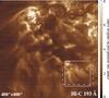 |
Fig. 1 Full field-of-view of the Hi-C observations. This image is taken in a wavelength band around 193 Å that under active region conditions is dominated by emission from Fe xii formed at around 1.5 MK. The core of the active region with several sunspots is located in the top half of the image (cf. Fig. 2). Here we concentrate on the loop system in the bottom right at the periphery of the active region. The regions indicated by the large solid square and the dashed rectangle are shown in Figs. 3 and 8. The small square shows the plage areas zoomed-in in Fig. 4. Here as in the following figures, the count rate is plotted normalized to the median value in the respective field-of-view. North is top. |
The paper is organized as follows. In Sect. 2 we introduce to the observations with Hi-C and their relation to the data from SDO in the Hi-C field of view. The miniature loops are discussed in Sect. 3.1 before we investigate the substructure of larger loops (Sect. 3.2) and the upper limit of the strands (Sect. 3.3), should loops not be monolithic. We then briefly turn to a comparison of the structures seen in Hi-C to those found in a 3D MHD model in Sect. 4, before we conclude our study.
2. Observations: Hi-C and AIA
Images of the corona with unprecedented spatial resolution have been obtained during a rocket flight by Hi-C. The instrument and first results are described by Kobayashi et al. (2013) and Cirtain et al. (2013). The Hi-C experiment recorded data in a wavelength band around 193 Å with 2 s exposure time. Under active region conditions this is dominated by emission from Fe xii (193 Å) originating at about 1.5 MK. The spatial scale is about 0.1′′ per pixel corresponding to 73 km/pixel. This is about a factor of 5.8 better than what is achieved by AIA/SDO, which is the current workhorse for solar coronal extreme-UV imaging studies. The temperature responses of the 193 Å channels of Hi-C and AIA are very similar. The effective area of HiC is approximately 5.3 times larger than that of AIA, though the Hi-C pixels cover an area that is roughly 36 times smaller.
In Fig. 1 we show the full field-of-view of the Hi-C observation1. This frame, which we investigate in this study, has been taken at around 18:54:16 UT on 11 July 2012. In this study we concentrate on the clear loop-structures in the lower righthand part of that image. This is in the periphery of the active region, away from the sunspots that are found in the upper half of the image (cf. Fig. 2).
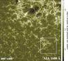 |
Fig. 2 Image of the chromosphere co-spatial and co-temporal with Fig. 1 taken by AIA in the 1600 Å channel. As in Fig. 1 the large and small squares indicate the field-of-view displayed in Fig. 3 and the zoom of the plage region in Fig. 4. |
 |
Fig. 3 Loop system at the periphery of the active region. This shows the 103′′ × 103′′ region indicated by the square in Fig. 1. The left panel shows the Hi-C observation (1000 × 1000 pixels), the right displays the data in the same wavelength channel (193 Å) recoded by AIA (173 × 173 pixels). The AIA image is spatially aligned with the Hi-C image and was taken at roughly the same time. The two squares here indicate regions that are magnified in Figs. 4 and 6 and that are located in areas dominated by a plage region and a loop system. |
The goal of this study is to investigate coronal features that are not resolvable with AIA. We thus compare the Hi-C image to an AIA image taken in the same 193 Å band only seconds after the Hi-C image. To align the images we had to compensate for a rotation of 1.9° and found the (linear) pixel scaling from Hi-C to AIA to be a factor of 5.81. For our analysis we also use images from the other AIA channels, all of which have been taken between 3 s before and 6 s after the Hi-C image. These we spatially scaled and aligned to match the AIA 193 Å image, and then applied the same rotation as for the 193 Å image to have a set of co-spatial images from Hi-C and AIA. We also make use of the magnetogram taken by the Helioseismic and Magnetic Imager (HMI/SDO; Scherrer et al. 2012) at 18:53:56, just 20 s before the Hi-C image. We scale, rotate and align the magnetogram to match the AIA 1600 Å image, so that it is also co-spatial with the Hi-C image.
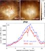 |
Fig. 4 Zoom of the plage region indicated in Fig. 3 by a square. The top two panels show the Hi-C image (150 × 150 pixel) and the AIA image (26 × 26 pixel) in that 15′′ × 15′′ region. The individual pixels are clearly identifiable in the AIA image. The bottom panel shows the variation in the count rate across the structures along the diagonal indicated by the dashed lines in the top panels. The pixels for the AIA data are indicated by diamonds. The bars indicate the individual pixels of Hi-C, the height of the bars represent the errors. For better comparison the AIA count rate is scaled by the factor given in the plot. The arrows in panels a) and c) indicate the position of a miniature coronal loop. See Sect. 3.1 |
3. Coronal structures
A rough inspection of the region-of-interest for our study as displayed in Fig. 3 already shows that parts of the Hi-C image look much crisper than the AIA 193 Å image, which is a clear effect of the improved spatial resolution of Hi-C. However, other parts of the image look quite alike, which is particularly true for the large loops in the middle of the region-of-interest.
3.1. Miniature coronal loops in plage region
To highlight that Hi-C shows miniature coronal loop-like structures almost down to its resolution limit, we first investigate a small region in the upper left of the region-of-interest, labeled “plage” in Fig. 3. A zoom of this area is shown in the top panels of Fig. 4. Here the increased spatial resolution of Hi-C is clearly evident. To emphasize this, panel c of Fig. 4 shows diagonal cuts through the Hi-C and AIA images in panels a and b. Prominent substructures are seen in the Hi-C image that are some seven to ten Hi-C pixels wide, corresponding to below 1′′. This corresponds to 1.5 AIA pixels and is therefore not resolved by AIA. Besides these, various intensity peaks are also visible, which are only two pixels wide, with the intensity enhancement clearly above the error level2. This confirms that Hi-C can detect small structures down to its resolution limit.
The nature of the small-scale intensity enhancements in the Hi-C 193 Å band needs some investigation. In Fig. 5 we plot the context of this small plage region in various AIA channels to investigate the connection throughout the atmosphere. The region of the strong brightening in 193 Å coincides with enhanced emission from the chromosphere as seen in the AIA 1600 Å channel (dominated by the Si i continuum). Even though this is not a pixel-to-pixel correlation, it is clear that the enhanced coronal emission occurs in a region with enhanced chromospheric activity. The emission in the 304 Å band dominated by the He ii line shows plasma below 105 K and is still closely related to the chromospheric network. The emission in the 131 Å, 171 Å, and 193 Å channels, which is dominated by plasma at 0.5 MK (Fe viii), 0.8 MK (Fe ix), and 1.5 MK (Fe xii), is very concentrated above one edge of the plage region. The image in the 211 Å channel (2.0 MK; Fe xiv) is almost identical to the 193 Å channel, which is why we do not include it here.
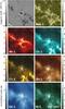 |
Fig. 5 Context of the plage region shown in Fig. 4. The AIA images in 7 channels show a 101′′ × 101′′ region and are taken within seconds of the 193 Å Hi-C image. The squares indicate the field-of-view shown in Fig. 4 and are co-spatial with the small squares in Fig. 3 labeled “plage”. In Fig. 4 the 193 Å images of Hi-C and AIA zooming into the small square are shown. Only there can the miniature loop be identifies in the Hi-C image. The top left panel shows the co-spatial line-of-sight magnetogram in the photosphere as seen by HMI, taken within seconds of the other images. See Sect. 3.1. |
This enhanced coronal emission in the plage area could either be due to small coronal loops within that region or could originate in footpoints of long hot loops rooted in that patch of enhanced magnetic field. However, the 335 Å and especially the 94 Å channels that should show hotter plasma – if it were be present – do not show any signature of a long hot loop rising from the patch in the center of the region. The 94 Å channel has two main contributions, one around 1.2 MK (Fe x) and another one at 7.5 MK (Fe xviii). However, the emission pattern in the 94 Å channel is very similar to the 171 Å channel, which indicates that there is relatively little plasma reaching temperatures of ≈7.5 MK along the line of sight. Likewise the 335 Å channel has main contributions around 0.1 MK, 1 MK, and 3 Mm, but lacks the signature of a long hot loop and shows more similarities to the 171 Å channel (albeit much noisier). For a detailed discussion of the temperature response of the AIA channels see (Boerner et al. 2012)3.
Unfortunately, there is no X-ray image taken at the same time and location. However, an inspection of an image from the Hinode X-ray telescope (XRT, Golub et al. 2007) taken about an hour before does not clearly resolve the issue. Therefore we assume that in the field of view of Fig. 5, the 193 Å emission in the center square is not moss-type emission from a large hot loop.
Based also on Hi-C data, Testa et al. (2013) see moss-type emission at the base of a hot (>5 MK) loop and find that it shows a high temporal variability. However, they look at a different part of the Hi-C field-of-view, which is near a footpoint of a hot loop. In contrast, the brightening we discuss here is not related to a hot loop, as outlined above.
If we can rule out that in our case the emission we see above the plage patch is coming from the footpoint of long hot loops, it has to come from small compact hot loops that close within the network patch. Such small loops are clearly not resolved by the AIA images. However, in the zoom to the Hi-C image of the plage area in Fig. 4a we can identify at least one structure that could be interpreted as a miniature hot loop that reaches temperatures of (at least) about 1.5 MK because we distinctively see it in the 193 Å channel of Hi-C (see arrows in panels a and c in Fig. 4). This loop would have a length (footpoint distance) of about only 1.5′′ corresponding to 1 Mm. For the width only an upper limit of 0.2 to 0.3′′ (150 km to 200 km) can be given, because the cross section of this structure is barely resolved.
The HMI magnetogram in Fig. 5 shows only one polarity in the plage area, which would argue against a miniature coronal loop (following the magnetic field lines). However, it could well be that small-scale patches of the opposite polarity are found in this plage area, too. These small-scale opposite polarities would then cancel out in the HMI observations with its limited spatial resolution. At least high-resolution observations (e.g. Wiegelmann et al. 2010), as well as numerical simulations of photospheric convection (e.g. Vögler et al. 2005), show small-scale opposite polarities in otherwise largely monopolar regions with footpoint distances on the order of 1 Mm or below. These small bipoles are the root of small flux tubes that have been found by Ishikawa et al. (2010) by inverting high-resolution spectro-polarimetry data. They found this flux tube with a footpoint distance of about 1 Mm to rise through the photosphere and then higher up into the atmosphere. These miniature loops could be related to the short transition region loops that are found to reside within the chromospheric network (Peter 2001).
From this discussion we can suggest that the small elongated structures we see in Hi-C above network and plage regions are in fact tiny loops reaching temperatures of 1.5 MK or more. These miniature coronal loops would have lengths (of their coronal part) of only around 1 Mm. If this is indeed the case, they would be interesting objects, because they would be so short that they would barely stick out of the chromosphere! Measuring from the photosphere, these loops would be only 5 Mm long, with a 2 Mm photosphere and chromosphere at each end. A 5 Mm long semi-circular loop has a footpoint distance of about 3 Mm. Such miniature loops would thus span across just a single granule, connecting the small-scale magnetic concentrations in the intergranular lanes.
These miniature loops might be a smaller version of X-ray bright points, which are enhancements of the X-ray emission related to small bipolar structures (Kotoku et al. 2007). Because of limitations of the spatial resolution of the X-ray observations (above 1′′) no X-ray bright points have been observed that are as small as the miniature loop reported here. Short loops have been studied theoretically (e.g. Müller et al. 2003; Sasso et al. 2012), indicating that such short hot structures are reasonable, even though these short model loops show peak temperatures of well below 1 MK. Klimchuk et al. (1987) found that hot short loops with heights below 1000 km are thermally unstable and evolve into cool loops with temperatures around 105 K. This would apply to the miniature loops proposed here, which would not be stable, anyway, because they can be expected to be disturbed rapidly by the convective motions of the granulation.
Future observational and modeling studies will have to show that this interpretation of miniature loops is correct, or the small-scale brightening in the plage region is better understood by the emission from the footpoint of a hot (≳3 MK) loop. In particular the upcoming Interface Region Imaging Spectrograph (IRIS; Wülser et al. 2012)4 with its high spatial resolution (0.3′′) covering emission from chromospheric to flare temperature will be well suited to investigate this from the observational side.
3.2. Substructure in large coronal loops
We now turn to the discussion of the substructure of larger coronal loops. In Fig. 3 a loop system is visible that connects the periphery of the active region to the surrounding network. In the following we concentrate on the small box labeled “loops” in Fig. 3, but our results apply to the other large loops in this figure. These loops show up in AIA 171 Å images but are faint in the AIA 211 Å band, which hints at a temperature of the loops in the range of 1 MK to 1.5 MK.
We chose this particular area of the Hi-C field-of-view because it is the area containing the most structures that can be easily identified as long coronal loops and that have arc lengths longer than about 50′′ (corresponding to 36 Mm). The northern part of the Hi-C field-of-view is dominated by plage and moss-type emission around the sunspots, as is clear from Figs. 1 and 2. This upper part is thus dominated by more compact structures. In the southern part of the image the region we selected shows the clearest loops. As also mentioned by Testa et al. (2013), the brightest emission seen by Hi-C originates in the plage and moss areas. The longer loops presumably reaching higher altitudes might have lower density and thus smaller emission when compared to the moss that originates in the footpoints of hotter loops.
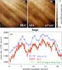 |
Fig. 6 Zoom of the loop region indicated in Fig. 3 by a square. Otherwise this is the same as Fig. 4. In addition, here the green line shows the cross-sectional cut averaged over 3′′ along the loops; i.e., it shows the average variation in the band defined by the two green lines in panel a). See Sect. 3.2. |
In panels a and b of Fig. 6 we show a zoom into this loop region, where the loops are seen passing roughly along the diagonal. In the AIA image (panel b) the individual pixels are clearly identifiable; this field of view consists of only 26 × 26 pixels. In contrast, the Hi-C image (150 × 150 pixels; panel a) shows a higher degree of noise. This is due to the lower count rate per pixel because of the higher spatial resolution, i.e., the smaller pixel size and the higher noise level of the Hi-C camera as compared to AIA. Still, from a comparison of the two images in panels a and b it is clear that the Hi-C image does not show a coherent substructure of the loops that is aligned with the loops.
This missing substructure of the loops in Fig. 6 becomes evident when investigating the cut perpendicular to the loops shown in panel c of Fig. 6. If one subtracted the background, the loops in AIA would have a width of some four pixels, i.e. they would be very close to the resolution limit of AIA. This size corresponds to some 1.8′′ to 2.4′′ or 1.3 Mm to 1.7 Mm. The cut of the Hi-C image confirms this width, which is very clear for the loops at spatial positions 5′′ and 10′′. Looking at AIA alone, one might have missed the small structure at 18′′ that is at the side of a bigger one. These results are consistent quantitatively and qualitatively with Brooks et al. (2013), who looked at short segments of a larger number of (long and short) loops.
Most importantly, the Hi-C data in panel c of Fig. 6 do not show any indication of a substructure of the loops that is sticking out of the noise (the Poisson errors are plotted as bars). When plotting the cross section of the loops not as a single-pixel cut, but averaged along the loops, the noise disappears and the loop cross-sections are smooth. The green line shows the variation in the 3′′ wide band defined by the green dashed lines in panel a. This averaging over 21 Hi-C pixels reduces the (Poisson) noise by a factor of about 4.5, giving a reduced error of about 20 counts5. This just corresponds to the variability still seen in the averaged cross-sectional cut. In Appendix B we give some further details on the size of the loops seen in Hi-C.
From the above we can conclude that within the instrumental capabilities of Hi-C, no plausible substructure of the long coronal loops can be seen, but the long loops are smooth and resolved. That we see structures in the Hi-C image in the plage area (Sect. 3.1) that are much smaller than the loop cross-sections reassures us that the spatial resolution of Hi-C is sufficient to see a substructure, if it both existed and were bright, and that the averaging process would reveal the structure if it were parallel to the arcsec-scale strands in the loops.
Of course, this observation does not rule out the possibility that the loops might have a substructure on scales than observable by Hi-C. Still, with these Hi-C observations we can set an upper limit for the diameter of individual strands that might compose single loops.
3.3. Upper limit for the diameter of strands in loops
In the following we estimate an upper limit for the thickness of the individual strands composing a coronal loop. For this we use the argument that the emission seen across the loop, i.e. the cross-sectional cut, should be smooth, just as found in the observations. We assume that all strands are circular in cross section and run in parallel. This is the simplest model possible, and certainly reality is much more complicated. However, for a rough estimation these assumptions should suffice.
We start with a loop with diameter D that is composed of a total number Nt of strands, each of which has the same diameter d (see Fig. 7). Of all the strands, only a fraction fb is bright, so that the number of bright strands is  (1)This fraction fb is equivalent to the fraction of time each individual strand with time-dependent heating, temperature and density structure is visible in a specific extreme ultraviolet (EUV) line or channel. Based on multi-stranded loop models, this fraction can be estimated to have an upper limit of fb ≈ 0.1 (e.g. Warren et al. 2003, 2008; Viall & Klimchuk 2011). The fraction fb is also equivalent to the volume-filling factor of the (bright) plasma in the corona. In observations of bright points Dere (2009) found values in the range of 0.003 to 0.3 with a median value of 0.04, which support our choice for an upper limit. One should remember that the filling factor might be much smaller, in particular when considering cooler plasma. For the transition region, Dere et al. (1987) found filling factors ranging from 0.01 down to 10-5.
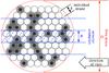 |
Fig. 7 Cartoon of the multi-stranded loop. The loop with diameter D is composed of many individual strands with diameter d. When observing the loop, each spatial resolution element of size R of the instrument corresponds to a column of the cross section. The hashed area represents one such column. Strands that are bright in a particular EUV channel (or line) are indicated by a back dot, and empty circles represent strands not radiating in this channel (at this instant in time). This example consists of Nt = 79 strands in total, of which Nb = 25 are bright, corresponding to a fraction fb = 0.3. For the loops on the Sun we estimate that they consist of Nt ≈ 2500 strands. See Sect. 3.3. |
When observing with an instrument with a spatial resolution R, each resolution element will represent a column of a cut through the loop (cf. Fig. 7). In this column there are Nc bright loops. To have a smooth cross-sectional profile we require that neighboring resolution elements contain a similar number of bright strands (each of the same brightness). The difference in the number of strands in neighboring resolution elements should then follow Poisson statistics,  . The relative difference in the number of strands in neighboring resolution elements gives the brightness variation directly, and for a smooth profile we require this to be smaller than ε,
 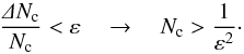 (2)Typically one would require ε ≈ 0.1, i.e., a pixel-to-pixel variation across the loop of less than 10% for a smooth profile.
From the number of bright strands in one column, Nc, we can estimate the number of bright strands in the whole loop, Nb, by the ratio of the cross section of the whole loop and of a single column (e.g. hashed column in Fig. 7), which together with Eq. (2) yields 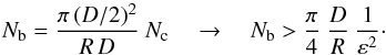 (3)Assuming that the strands in the loop are packed as densely as possible, the cross section of the loop as a whole and of the Nt strands are related by
  (4)where the factor of
  stems from the densest packing of circles in a plane. Using Eqs. (1) and (3) this now gives the upper limit for the diameter of individual strands,
 ![\begin{equation} \label{E:strand.limit} d ~~ < ~~ \frac{2\sqrt{2}\sqrt[4~]{3}}{\pi} ~~ \varepsilon ~ \sqrt{f_{\rm b}} ~~ \sqrt{R\,D} ~~~ \approx ~~~ 1.2 ~ \sqrt{f_{\rm b}} ~ \varepsilon ~\sqrt{R\,D} , \end{equation}](/articles/aa/full_html/2013/08/aa21826-13/aa21826-13-eq31.png) (5)and the lower limit for the total number os strands in the loop,
(5)and the lower limit for the total number os strands in the loop,  (6)For the loops observed here with a diameter of D ≈ 2′′ and the resolution of Hi-C of R ≈ 0.2′′ assuming a fraction of the bright loops of fb ≈ 0.1 and a pixel-to-pixel variation of ε ≈ 0.1 in the observation, we find an upper limit for the diameter of an individual strand of d ≈ 0.025′′ corresponding to about
  (7)This strand diameter of only 15 km is small compared to the loop diameter – this loop would have to host at least about Nt ≈ 7500 strands of which Nb ≈ 750 are bright in the given EUV channel at any given time. In Appendix C we discuss a simple numerical experiment confirming this conclusion. If one adopted the lower value of 0.003 for the filling factor derived by Dere (2009), one would end up with a quarter million strands with diameters of only 3 km.
Strictly speaking, this discussion applies only for the 193 Å channel. Other bandpasses respond differently to different heating scenarios in loop models (e.g., see the review of Reale 2010) and thus might show different filling factors. Still, our results can be expected to apply roughly to emission originating in the coronal plasma at 1 MK to 2 MK.
Together with the discussion in Sect. 3.2, we conclude that the loops are either monolithic structures, the diameter of the individual strands has to be smaller than 15 km, or else the strands must be implausibly well organized. This new upper limit is more than a factor of 10 smaller than derived from previous studies (e.g. Brooks et al. 2012), which became possible by the enhanced spatial resolution of Hi-C. The multi-stranded loop scenario can only be valid if the upper limit of the strands set by observations is higher than the lower limit for the strand diameter set by basic physical processes such as reconnection, gyration, heat conduction, or turbulence. At this point we think that this is the case; however, more detailed studies, in particular of MHD turbulence, would be needed for a final conclusion. We discuss these issues briefly in Appendix A.
 |
Fig. 8 Morphological comparison of observation and model. The top panel shows the actual observation of Hi-C (193 Å band). The field of view (124′′ × 62′′) is outlined in Fig. 1 by the dashed rectangle. The bottom panel shows the coronal emission as synthesized from a 3D MHD model for this channel (165 × 109 Mm). The arrows point to features that can be found in both model and observations: a) expanding envelope that consists of several non-expanding loops; b) thin non-expanding threads; and c) rather broad loop-like structures with approximately constant cross section. See Sect. 4. |
4. Loop morphology and comparison to a 3D model
In a first attempt at a morphological comparison between the Hi-C observations and a 3D coronal model, we just highlight some common features between observation and model on a qualitative basis. For final conclusions, a more detailed quantitative comparison is needed, and in particular, a more in-depth analysis of the model is required to better understand how the various structures form.
The coronal loops in the field-of-view of the Hi-C observations discussed in this manuscript can be classified (by eye) into three categories (cf. Fig. 8, top panel):
-
(a)
Expanding envelope that consists of several non-expandingloops,
-
(b)
thin (≲3′′) non-expanding threads,
-
(c)
broad (≳5′′) loop-like structures with approximately constant cross section.
The individual loops in the expanding structure (a) and the thin threads (b) seem to show no (significant) expansion. We are investigating this quantitatively with the Hi-C data and will present our results in a separate paper. The tendency for constant cross-section was reported more than a decade ago for loops observed in the EUV and X-rays (Klimchuk 2000; Watko & Klimchuk 2000; López Fuentes et al. 2006). Recently, based on a 3D MHD model, it has been shown that the constant cross section could be due to the temperature and density structure within in the expanding magnetic structure, in interplay with the formation of the coronal emission lines (Peter & Bingert 2012). This would work for EUV observations, but it still has to be investigated whether this would also work at X-ray wavelengths that come from a much broader range of high temperatures.
Recently, Malanushenko & Schrijver (2013) have suggested that the constant cross section result may be an artifact of the observing geometry and the likelihood that the shape of the cross section varies along the loop. The cross sectional area could expand, but if it does so primarily along the line-of-sight, then the loop thickness in the plane-of-the sky (i.e., the image) will be constant. This could certainly explain many loops. However, there should be many other cases where a different observing geometry reveals very strong expansion. Such cases need to be verified before we can accept this explanation for the constant cross section loops. Also, the thermal structure along and perpendicular to the loops has to be considered, and not the magnetic structure alone, as pointed out by Mok et al. (2008) and Peter & Bingert (2012).
Because the 3D MHD model successfully provided a match to the constant cross-section loops, we compared a snapshot of a 3D MHD model to the Hi-C observation to see if we also find the three categories of loop structures in the emission synthesized from the model. In the 3D MHD we solve the mass, momentum, and energy balance in a box spanning 167 × 167 Mm2 horizontally and 80 Mm in the vertical direction (5123 equidistant grid). Horizontal motions (of the granulation) drive the magnetic field in the photosphere and lead to braiding of magnetic field lines as originally suggested by Parker (1972). This process induces currents that are dissipated in the upper atmosphere and by this heat the corona. The details of this model have been described by Bingert & Peter (2011, 2013). The numerical experiment we use here differs from that model by the magnetic field at the lower boundary, an increased size of the computational domain, and a higher spatial resolution. As described by Peter et al. (2006), we interpolate the MHD quantities to avoid aliasing effects and compute the emission as would be seen by AIA using the temperature response functions (Boerner et al. 2012; Peter & Bingert 2012). In Fig. 8 we show the synthesized emission in the 193 Å channel6 integrated along the vertical axis, i.e., when looking from straight above.
In the image synthesized from the model we find the same three classes of structures as in the actual observation; the labeled arrows point at such structures. While the thin constant-cross-section loops (b) have been discussed before (Peter & Bingert 2012), here we also find the non-expanding loops in an expanding envelope (a) and the broad loop-like structures (c). It is beyond the scope of this (mainly observational) study to perform a detailed analysis of the 3D MHD model to investigate what the nature of these three categories is. Here we simply state that these categories are also found in numerical experiments, so that there is some hope of understanding how they come about in future studies.
5. Conclusions
We presented results on the structure of coronal loops based on new observations with the Hi-C rocket telescope that provides unprecedented spatial resolution in the EUV down to 0.2′′ on a spatial scale of 0.1′′ per pixel. Our main conclusions are the following:
We have found miniature loops hosting plasma at 1.5 MK with a length of only about 1 Mm and a thickness below 200 km (Sect. 3.1). With other current instrumentation, such as AIA, these would cover just two spatial pixels. These miniature loops are consistent with small magnetic flux tubes that have been observed to rise through the photosphere into the upper atmosphere. However, it will be a challenge to understand these miniature loops in terms of a (traditional) one-dimensional model. From the observational side, this clearly shows the need for future high-resolution Hi-C-type observations, together with high-resolution spectro-polarimetric observations of the photosphere and chromosphere.
In the case of the longer more typical coronal loops we found that the Hi-C observations do not show indications of a substructure in these loops (Sect. 3.2). Therefore those loops with diameters of typically 2′′ to 3′′ are either real monolithic entities or they would have to be composed of many strands with diameters well below the resolution limit of Hi-C. Based on some simple assumptions, we found that the strands would have to have a diameter of at most 15 km, which would imply that a loop with 2′′ diameter would have to be composed of at least 7500 individual strands (Sect. 3.3). This would compare to a 1 cm diameter wire rope consisting of wire strands of only 0.1 mm diameter. Regardless of whether the loops are monolithic or multi-stranded in nature, it still remains puzzling what determines the width of the loop of typically 2′′ to 3′′, which is found consistently in both the Hi-C and the AIA data. The observational time and field-of-view of the Hi-C rocket experiment were limited, so this discussion cannot be generalized. This highlights the need for such high-resolution observations of the corona in future space missions.
Numerical experiments show similar (large) loop structures as found in the Hi-C observations: non-expanding loops in expanding envelopes, thin threads, and thick constant cross-section loops. It still needs to be determined how these are produced in the numerical experiments and whether the processes in the model can be realistically applied to the real Sun. Either way, the 3D numerical experiments provide us with a tool for investigating this in future studies and thus learn more about the nature of loops in the corona, both miniature and large.
Online material
Appendix A: Lower limit for the strand diameter
The typical length scale perpendicular to the magnetic field through whatever process places a lower limit for the strand diameter d. If d were smaller than this length scale, the neighboring strand would interact through this process and consequently the strands would no longer be individual structures but one common entity. This discussion is of interest, because if this lower limit for the strand diameter were larger than the upper limit derived from observations in Sect. 3.3, the loops would have to be monolithic structures.
Reconnection.
Most probably reconnection is the basis of the heating process. For reconnection to happen the inductive term and the dissipative term in the induction equation have to be on the same order of magnitude, or in other words, the magnetic Reynolds number has to be of order unity; i.e., Rm = U ℓ/η ≈ 1. Here U is the typical velocity and η the magnetic diffusivity. The length scale ℓ would represent the thickness of the resulting current sheet. This ℓ is then a lower limit for the strand diameter. If strands were thinner, they would be part of the same reconnection region and thus not distinguishable.
Following Spitzer (1962) one can derive the electric conductivity σ from classical transport theory, which then provides η = (μ0 σ)-1. In the corona at 106 K, the value is η ≈ 1 m2 s-1. For Rm ≈ 1 the length scale is given by ℓ ≈ η/U. For a low value of U ≈ 1 km s-1 (certainly there are much faster flows in the corona), we find a value of  (A.1)Arguments along this line of thought can be found in e.g. Boyd & Sanderson (2003) or in the preface of Ulmschneider et al. (1991). This value must be a vast underestimation, because it is much less than the ion (and even the electron) gyro radius.
Gyration.
Another relevant length scale is the Larmor or gyro radius of the gyration of the ions and electrons in the corona. This is given by rL = m v⊥(e B)-1 , with mass m and charge e of the particles and the magnetic field B. Assuming that the perpendicular velocity is given by the thermal speed, v⊥ = (3kT/m)1/2, one finds  (A.2)Thus in the corona at temperatures of about T ≈ 106 K and for B ≈ 10 G, the Larmor radius of the protons is on the order of 1 m.
Heat conduction.
The head conduction perpendicular to the magnetic field is much less efficient than the parallel conduction, but if the temperature gradients across the field become large enough it might become non-negligible. For the coefficient of the perpendicular heat conduction one can derive (e.g. Priest 1982, Sect. 2.3.2) ![\appendix \setcounter{section}{1} \begin{eqnarray} \nonumber \kappa_\perp = 3.6\times10^{-8}\, \frac{\rm W}{\rm ~K~m~} ~ \frac{~ \big(n\,[10^{15}\,{\rm{m}}^{-3}]\big)^2 ~~ }{~\big(T\,[10^{6}\,{\rm{K}}]\big)^{1/2} ~~ \big(B\,[10\,{\rm{G}}]\big)^{2} ~~ \ln\mathit{\Lambda} ~} , \\ \label{E:heat.perp} \end{eqnarray}](/articles/aa/full_html/2013/08/aa21826-13/aa21826-13-eq63.png) (A.3)where n is the particle density and in the corona the Coulomb logarithm is roughly lnΛ ≈ 13.
(A.3)where n is the particle density and in the corona the Coulomb logarithm is roughly lnΛ ≈ 13.
We now consider the minimum diameter d of a strand with length L. For this we assume that the energy lost by heat conduction perpendicular to the magnetic field, κ⊥ ∇T, through the mantle surface of the strand, L πd, is balanced by the energy input FH through the two footpoints of the strand with cross section πd2/4,  (A.4)Using expression (A.3) one finds
 ![\appendix \setcounter{section}{1} \begin{eqnarray} \nonumber d ~>~ 23\,{\rm{m}}~~\frac{~ n\,[10^{15}\,{\rm{m}}^{-3}] ~~ \big(T\,[10^{6}\,{\rm{K}}]\big)^{\!1/4} ~~ \big(L\,[100\,{\rm{Mm}}]\big)^{\!1/2} }{B\,[10\,{\rm{G}}] ~~ \big(F_{\rm H}\,[1000\,{\rm{W}}\,{\rm{m}}^{-2}]\big)^{\!1/2}} \cdot \\ \label{E:lower.limit} \end{eqnarray}](/articles/aa/full_html/2013/08/aa21826-13/aa21826-13-eq72.png) (A.5)For typical coronal values and an energy flux density into the corona of 1000 W m-2, we find a diameter of the order of 20 m. This is a lower limit for the strand diameter. If the strand were thinner, the temperature gradient to the neighboring (cold) strand would be higher, and thus the energy loss by perpendicular heat conduction would be stronger than the energy input. Consequently the strand would start to dissolve into the neighboring strands, thereby increasing its diameter.
(A.5)For typical coronal values and an energy flux density into the corona of 1000 W m-2, we find a diameter of the order of 20 m. This is a lower limit for the strand diameter. If the strand were thinner, the temperature gradient to the neighboring (cold) strand would be higher, and thus the energy loss by perpendicular heat conduction would be stronger than the energy input. Consequently the strand would start to dissolve into the neighboring strands, thereby increasing its diameter.
Other processes.
From the above discussion we find that the strands should be at least some 10 m to 50 m in diameter, set by the perpendicular heat conduction. However, this lower limit might be on the low side. Other processes, in particular MHD turbulence, might increase the length scale perpendicular to the magnetic field considerably. Then the reconnection process will effectively operate on larger length scales, and also the heat conduction perpendicular to the magnetic field will be more effective, ensuring smaller temperature gradients and thus larger length scales perpendicular to the magnetic field. The MHD turbulence simulations of Rappazzo et al. (2008) show elongated current concentrations aligned with the magnetic field, which could be interpreted as the strands in a loop. However, because of the lack of heat conduction and radiative losses in their model, which would have been beyond the scope of their study, one cannot say much about the diameter of the potentially developing strands.
Future theoretical investigations might place a better lower limit to the strand diameter and thus further limit the range of possible strand diameters given by the relations (7) and (A.5). Finally such studies would help in deciding whether loops are monolithic or multi-stranded.
Appendix B: Size of the loops seen in Hi-C
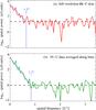 |
Fig. B.1 Size of the loop structures in Hi-C. Shown are the power spectra of the cross-sectional cuts of the loops in Fig. 6, for the original data (top panel, red here and in Fig. 6) and the data averaged over 21 pixels along the loop (bottom panel green here and in Fig. 6). The horizontal dashed lines shows the noise level (21 in top panel, 1 in bottom panel). The diagonal blue line is a by-eye fit to the power spectrum at low spatial frequencies, the vertical line indicated the intersection of this fit with the respective noise level. The numbers in the panels give the corresponding spatial scale. See Appendix B. |
To obtain a quantitative estimate for the size of the loop structures discussed in Sect. 3.2 we performed a Fourier transform of the spatial variation shown in Fig. 6. We did this for the original profile across the loop (red with bars in Fig. 6), as well as for the data-averaged 21 pixels along the loops (in green). After subtracting the linear trend and apodizing using a Welsh filter we performed a Fourier transform to obtain the power spectrum as a function of spatial frequency. The resulting power spectra are shown in Fig. B.1. The top panel shows the power spectrum for the original profile, the bottom panel shows the power spectrum for the averaged data.
We calculated the noise level in the power spectrum by equating the square of the error in the data integrated over space to the noise in the power integrated over spatial frequency. For the data averaged aver 21 pixels along the loop, we assumed the error to be given by the original errors scaled down by  . We have overplotted these noise levels for the original and the spatially averaged data in Fig. B.1.
From the power spectra in Fig. B.1, it is clear that all structures on scales below 1.2′′ are consistent with noise (i.e., right of the vertical blue lines). The corresponding frequency of 0.8 1/′′ is far from the Nyquist frequency of about 3.4 1/′′. The results are similar for the original and the averaged Hi-C data. Based on the averaged Hi-C data, which show less noise, the structures on scales below 1.2′′ represent less than 1% of the power. If there were significant power from (sub-)structures in the loops investigated in Fig. 6, it should show up somewhere in the frequency range from 1 1/′′ to 3.4 1/′′, where Hi-C would be sensitive.
In other parts of the field-of-view for different structures, e.g. in moss areas or for the miniature loop discussed in Sect. 3.1, Hi-C shows much smaller structures basically down to its resolution limit. However, the loop structures investigated in Sect. 3.2 and Fig. 6, which have widths of about 2′′, do not show any substructure on scales below 1.2′′. This is equivalent to saying that the long 2′′ wide coronal loops as seen in Hi-C have no substructure.
Appendix C: Appearance of multi-stranded loops
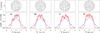 |
Fig. C.1 Numerical experiments for the cross-sectional profile of multi-stranded loops. The top panels show the loop cross-section for four experiments with about 7500 strands where about 750 are bright. They differ only by the random selection of which strands are bright. Each strand has a diameter of 15 km. The bottom panels show the respective cross-sectional profiles (i.e., integration along Y) as would be observed by AIA (blue, diamonds) and Hi-C (red). The height of the bars for Hi-C correspond to 10% of the counts. See Appendix C. |
To visualize the analytical results in Sect. 3.3 on the upper limit for the strand diameter and the lower limit for the number of
bright strands in the loop, we conducted a simple numerical experiment. In the following all variables have the same meaning as in Sect. 3.3.
For the experiment we assumed each individual strand has a Gaussian cross-sectional profile (in intensity), where the full width at half maximum is used to define the strand diameter d. We then filled the circular loop cross section with a most dense packing of circles, which provides us with the total number of strands Nt. For the numerical experiment we randomly selected which of the loops are bright, with a fraction fb of all loops being bright, Nb = Nt fb.
We then integrated along a line-of-sight perpendicular to the loop, which provides the cross-sectional intensity profile of the loop. This profile was folded with a point spread function for AIA and Hi-C (where for simplicity we assumed a Gaussian profile, which is sufficient for the purpose at hand).
In Fig. C.1 we visualize the results for the parameters as found in Sect. 3.3, i.e., a total of Nt = 7500 strands of which a fraction of fb = 0.1 or Nb = 750 is bright with a diameter of d = 15 km. These fit into a circular loop with a diameter D corresponding to 2′′ or 1500 km.
In the top panels of Fig. C.1 we show the cross section of the loop for four different random selections of which loops are bright. The respective lower panel shows the cross-sectional profile if it were observed with AIA or Hi-C. It is clear that the limited spatial resolution of AIA of slightly worse than 1′′ does not allow any features to be seen. We instead see a smooth profile that is basically identical for all four cases.
The Hi-C data show some variation in the cross-sectional profile. In Sect. 3.3 we used the variability ε to derive the upper limit of the strand diameter. Here we plot the variability ε as bars on top of the profile. We see that the variability in the simulated cross-sectional profile for the four cases in Fig. C.1 is roughly comparable with the variability ε we used in Sect. 3.3. If we used a significantly larger (smaller) number of individual strands, we would find a smoother (rougher) cross sectional profile, which confirms the derivation of the limit for the strand diameter in Sect. 3.3. Actually, the cross sectional profiles shown in Fig. C.1 look quite similar to the profiles of the loops seen in observations in Fig. 6.
This numerical experiment also elucidates the interpretation of substructures in loops. In the four examples we show in Fig. C.1 only one (d) shows a perfectly smooth profile. One might be tempted to conclude from a cross-sectional profile, as in case (c), that this loop shows only two major substructures. In cases (a) and (b) one might underestimate the diameter of the loop. Looking at more randomly generated distributions of bright strands, one finds a wide variety of cross-sectional profiles. This shows that one has to be careful when analyzing single loops, because the (random) distribution of a large number of loops might mimic the existence of structures that are not present in reality.
These numerical experiments confirm our conclusions based on the analytical analysis in Sect. 3.3 that the strand diameter should be on the order of about 15 km or less (in particular when conducting experiments for loops with different numbers of strands, which we do not show here for brevity). Of course, this does not exclude the possibility that there is no substructure at all, but rather that the loop is a monolithic structure, as noted in Sect. 3.3.
The data are available through the Virtual Solar Observatory (VSO) at http://www.virtualsolar.org/.
One could also speculate that the AIA short wavelength channels might show mainly cool transition region emission; in particular, the 193 Å and 211 Å channels have a significant contribution from temperatures around 0.2 MK (O v) in quiet Sun conditions. However, then these two channels should share some characteristics with the 304 Å channel, which they do not. In fact, the brightening in 193 Å and 211 Å does not overlap at all with the pattern in 304 Å. Thus we can conclude that the 193 Å and 211 Å channels really show plasma primarily at 1.5 MK to 2 MK.
Launched on 27. June 2013. See also http://iris.lmsal.com
Alternatively one could have averaged in time or in both time and space. For the case at hand this averaging along the loops seems appropriate because the loops in Fig. 6 show a nice smooth variation along the loop.
Acknowledgments
We acknowledge the High-resolution Coronal Imager instrument grant funded by the NASA’s Low Cost Access to Space program. MSFC/NASA led the mission and partners include the Smithsonian Astrophysical Observatory in Cambridge, Mass.; Lockheed Martin’s Solar Astrophysical Laboratory in Palo Alto, Calif.; the University of Central Lancashire in Lancashire, England; and the Lebedev Physical Institute of the Russian Academy of Sciences in Moscow. The AIA and HMI data used are provided courtesy of NASA/SDO and the AIA and HMI science teams. The AIA and HMI data have been retrieved using the German Data Center for SDO. The numerical simulation was conducted at the High Performance Computing Center Stuttgart (HLRS). This work was partially funded by the Max-Planck/Princeton Center for Plasma Physics. The work of J.A.K. was supported by the NASA Supporting Research and Technology and Guest Investigator Programs. H.P. acknowledges stimulating discussions with Robert Cameron and Aaron Birch. We thank the anonymous referee for constructive comments.
References
- Antolin, P., & Rouppe van der Voort, L. 2012, ApJ, 745, 152 [NASA ADS] [CrossRef] [Google Scholar]
- Aschwanden, M. J., & Boerner, P. 2011, ApJ, 732, 81 [NASA ADS] [CrossRef] [Google Scholar]
- Bingert, S., & Peter, H. 2011, A&A, 530, A112 [NASA ADS] [CrossRef] [EDP Sciences] [Google Scholar]
- Bingert, S., & Peter, H. 2013, A&A, 550, A30 [NASA ADS] [CrossRef] [EDP Sciences] [Google Scholar]
- Boerner, P. F., Edwards, C. G., Lemen, J. R., et al. 2012, Sol. Phys., 275, 41 [NASA ADS] [CrossRef] [Google Scholar]
- Boyd, T. J. M., & Sanderson, J. J. 2003, The Physics of Plasmas (Cambridge University Press) [Google Scholar]
- Bray, R. J., Cram, L. E., Durrant, C., & Loughhead, R. E. 1991, Plasma Loops in the Solar Corona (Cambridge University Pres) [Google Scholar]
- Brooks, D. H., Warren, H. P., & Ugarte-Urra, I. 2012, ApJ, 755, L33 [NASA ADS] [CrossRef] [Google Scholar]
- Brooks, D. H., Warren, H. P., Ugarte-Urra, I., & Winebarger, A. R. 2013, ApJ, 772, L19 [NASA ADS] [CrossRef] [Google Scholar]
- Cargill, P. J. 1994, ApJ, 422, 381 [Google Scholar]
- Cirtain, J. W., Golub, L., Winebarger, A. L., et al. 2013, Nature, 493, 501 [NASA ADS] [CrossRef] [Google Scholar]
- Del Zanna, G., & Mason, H. E. 2003, A&A, 406, 1089 [NASA ADS] [CrossRef] [EDP Sciences] [Google Scholar]
- Dere, K. P. 2009, A&A, 497, 287 [NASA ADS] [CrossRef] [EDP Sciences] [Google Scholar]
- Dere, K. P., Bartoe, J.-D. F., Brueckner, G. E., Cook, J. W., & Socker, D. G. 1987, Sol. Phys., 114, 223 [NASA ADS] [CrossRef] [Google Scholar]
- Feldman, U., Dammasch, I. E., Wilhelm, K., et al. 2003, SUMER atlas – Images of the solar upper atmosphere from SUMER on SOHO (ESA Publications Div.), ESA SP, 1274 [Google Scholar]
- Golub, L., Deluca, E., Austin, G., et al. 2007, Sol. Phys., 243, 63 [NASA ADS] [CrossRef] [Google Scholar]
- Gudiksen, B., & Nordlund, Å. 2005, ApJ, 618, 1031 [NASA ADS] [CrossRef] [Google Scholar]
- Ishikawa, R., Tsuneta, S., & Jurčák, J. 2010, ApJ, 713, 1310 [NASA ADS] [CrossRef] [Google Scholar]
- Klimchuk, J. A. 2000, Sol. Phys., 193, 53 [NASA ADS] [CrossRef] [Google Scholar]
- Klimchuk, J. A., Antiochos, S. K., & Mariska, J. T. 1987, ApJ, 320, 409 [NASA ADS] [CrossRef] [Google Scholar]
- Kobayashi, K., Cirtain, J., R., W. A., et al. 2013, Sol. Phys., submitted [Google Scholar]
- Kotoku, J., Kano, R., Tsuneta, S., et al. 2007, PASJ, 59, 735 [Google Scholar]
- Lemen, J., Title, A. M., Akin, D. J., et al. 2012, Sol. Phys., 275, 14 [Google Scholar]
- López Fuentes, M. C., Klimchuk, J. A., & Démoulin, P. 2006, ApJ, 639, 459 [NASA ADS] [CrossRef] [Google Scholar]
- López Fuentes, M. C., & Klimchuk, J. A. 2010, ApJ, 719, 591 [NASA ADS] [CrossRef] [Google Scholar]
- Malanushenko, A., & Schrijver, C. J. 2013, ApJ, in press [Google Scholar]
- Mok, Y., Mikić, Z., Lionello, R., & Linker, J. A. 2008, ApJ, 679, L161 [NASA ADS] [CrossRef] [Google Scholar]
- Müller, D., Hansteen, V. H., & Peter, H. 2003, A&A, 411, 605 [NASA ADS] [CrossRef] [EDP Sciences] [Google Scholar]
- Parker, E. N. 1972, ApJ, 174, 499 [NASA ADS] [CrossRef] [Google Scholar]
- Parker, E. N. 1983, ApJ, 264, 642 [NASA ADS] [CrossRef] [Google Scholar]
- Parker, E. N. 1988, ApJ, 330, 474 [Google Scholar]
- Pesnell, W. D., Thompson, B. T., & Chamberlin, P. C. 2012, Sol. Phys., 275, 3 [NASA ADS] [CrossRef] [Google Scholar]
- Peter, H. 2001, A&A, 374, 1108 [NASA ADS] [CrossRef] [EDP Sciences] [Google Scholar]
- Peter, H., & Bingert, S. 2012, A&A, 548, A1 [NASA ADS] [CrossRef] [EDP Sciences] [Google Scholar]
- Peter, H., Gudiksen, B., & Nordlund, Å. 2006, ApJ, 638, 1086 [NASA ADS] [CrossRef] [MathSciNet] [Google Scholar]
- Poletto, G., Vaiana, G. S., Zombeck, M. V., Krieger, A. S., & Timothy, A. F. 1975, Sol. Phys., 44, 83 [NASA ADS] [CrossRef] [Google Scholar]
- Priest, E. R. 1982, Solar Magnetohydrodynamics (Dordrecht: D. Reidel) [Google Scholar]
- Rappazzo, A. F., Velli, M., Einaudi, G., & Dahlburg, R. B. 2008, ApJ, 677, 1348 [NASA ADS] [CrossRef] [Google Scholar]
- Reale, F. 2010, Liv. Rev. Sol. Phys., 7, 5 [Google Scholar]
- Sasso, C., Andretta, V., Spadaro, D., & Susino, R. 2012, A&A, 537, A150 [NASA ADS] [CrossRef] [EDP Sciences] [Google Scholar]
- Scherrer, P. H., Schou, J., Bush, R. I., et al. 2012, Sol. Phys., 275, 207 [Google Scholar]
- Spitzer, L. 1962, Physics of fully ionized gases, 2nd edn (New York: Interscience) [Google Scholar]
- Testa, P., De Pontieu, B., Martïnez-Sykora, J., et al. 2013, ApJ, 770, L1 [NASA ADS] [CrossRef] [Google Scholar]
- Ulmschneider, P., Priest, E. R., & Rosner, R. 1991, Mechanisms of chromospheric and coronal heating (Berlin: Springer-Verlag) [Google Scholar]
- Viall, N. M., & Klimchuk, J. A. 2011, ApJ, 738, 24 [Google Scholar]
- Vögler, A., Shelyag, S., Schüssler, M., et al. 2005, A&A, 429, 335 [NASA ADS] [CrossRef] [EDP Sciences] [Google Scholar]
- Warren, H. P., Winebarger, A. R., & Mariska, J. T. 2003, ApJ, 593, 1174 [NASA ADS] [CrossRef] [Google Scholar]
- Warren, H. P., Ugarte-Urra, I., Doschek, G. A., Brooks, D. H., & Williams, D. R. 2008, ApJ, 686, L131 [NASA ADS] [CrossRef] [Google Scholar]
- Watko, J. A., & Klimchuk, J. A. 2000, Sol. Phys., 193, 77 [NASA ADS] [CrossRef] [Google Scholar]
- Wiegelmann, T., Solanki, S. K., Borrero, J. M., et al. 2010, ApJ, 723, L185 [NASA ADS] [CrossRef] [EDP Sciences] [Google Scholar]
- Wülser, J.-P., Title, A. M., Lemen, J. R., et al. 2012, in SPIE Conf. Ser., 8443.008 [Google Scholar]
All Figures
|
Fig. 1 Full field-of-view of the Hi-C observations. This image is taken in a wavelength band around 193 Å that under active region conditions is dominated by emission from Fe xii formed at around 1.5 MK. The core of the active region with several sunspots is located in the top half of the image (cf. Fig. 2). Here we concentrate on the loop system in the bottom right at the periphery of the active region. The regions indicated by the large solid square and the dashed rectangle are shown in Figs. 3 and 8. The small square shows the plage areas zoomed-in in Fig. 4. Here as in the following figures, the count rate is plotted normalized to the median value in the respective field-of-view. North is top. |
| In the text | |
|
Fig. 2 Image of the chromosphere co-spatial and co-temporal with Fig. 1 taken by AIA in the 1600 Å channel. As in Fig. 1 the large and small squares indicate the field-of-view displayed in Fig. 3 and the zoom of the plage region in Fig. 4. |
| In the text | |
|
Fig. 3 Loop system at the periphery of the active region. This shows the 103′′ × 103′′ region indicated by the square in Fig. 1. The left panel shows the Hi-C observation (1000 × 1000 pixels), the right displays the data in the same wavelength channel (193 Å) recoded by AIA (173 × 173 pixels). The AIA image is spatially aligned with the Hi-C image and was taken at roughly the same time. The two squares here indicate regions that are magnified in Figs. 4 and 6 and that are located in areas dominated by a plage region and a loop system. |
| In the text | |
|
Fig. 4 Zoom of the plage region indicated in Fig. 3 by a square. The top two panels show the Hi-C image (150 × 150 pixel) and the AIA image (26 × 26 pixel) in that 15′′ × 15′′ region. The individual pixels are clearly identifiable in the AIA image. The bottom panel shows the variation in the count rate across the structures along the diagonal indicated by the dashed lines in the top panels. The pixels for the AIA data are indicated by diamonds. The bars indicate the individual pixels of Hi-C, the height of the bars represent the errors. For better comparison the AIA count rate is scaled by the factor given in the plot. The arrows in panels a) and c) indicate the position of a miniature coronal loop. See Sect. 3.1 |
| In the text | |
|
Fig. 5 Context of the plage region shown in Fig. 4. The AIA images in 7 channels show a 101′′ × 101′′ region and are taken within seconds of the 193 Å Hi-C image. The squares indicate the field-of-view shown in Fig. 4 and are co-spatial with the small squares in Fig. 3 labeled “plage”. In Fig. 4 the 193 Å images of Hi-C and AIA zooming into the small square are shown. Only there can the miniature loop be identifies in the Hi-C image. The top left panel shows the co-spatial line-of-sight magnetogram in the photosphere as seen by HMI, taken within seconds of the other images. See Sect. 3.1. |
| In the text | |
|
Fig. 6 Zoom of the loop region indicated in Fig. 3 by a square. Otherwise this is the same as Fig. 4. In addition, here the green line shows the cross-sectional cut averaged over 3′′ along the loops; i.e., it shows the average variation in the band defined by the two green lines in panel a). See Sect. 3.2. |
| In the text | |
|
Fig. 7 Cartoon of the multi-stranded loop. The loop with diameter D is composed of many individual strands with diameter d. When observing the loop, each spatial resolution element of size R of the instrument corresponds to a column of the cross section. The hashed area represents one such column. Strands that are bright in a particular EUV channel (or line) are indicated by a back dot, and empty circles represent strands not radiating in this channel (at this instant in time). This example consists of Nt = 79 strands in total, of which Nb = 25 are bright, corresponding to a fraction fb = 0.3. For the loops on the Sun we estimate that they consist of Nt ≈ 2500 strands. See Sect. 3.3. |
| In the text | |
|
Fig. 8 Morphological comparison of observation and model. The top panel shows the actual observation of Hi-C (193 Å band). The field of view (124′′ × 62′′) is outlined in Fig. 1 by the dashed rectangle. The bottom panel shows the coronal emission as synthesized from a 3D MHD model for this channel (165 × 109 Mm). The arrows point to features that can be found in both model and observations: a) expanding envelope that consists of several non-expanding loops; b) thin non-expanding threads; and c) rather broad loop-like structures with approximately constant cross section. See Sect. 4. |
| In the text | |
|
Fig. B.1 Size of the loop structures in Hi-C. Shown are the power spectra of the cross-sectional cuts of the loops in Fig. 6, for the original data (top panel, red here and in Fig. 6) and the data averaged over 21 pixels along the loop (bottom panel green here and in Fig. 6). The horizontal dashed lines shows the noise level (21 in top panel, 1 in bottom panel). The diagonal blue line is a by-eye fit to the power spectrum at low spatial frequencies, the vertical line indicated the intersection of this fit with the respective noise level. The numbers in the panels give the corresponding spatial scale. See Appendix B. |
| In the text | |
|
Fig. C.1 Numerical experiments for the cross-sectional profile of multi-stranded loops. The top panels show the loop cross-section for four experiments with about 7500 strands where about 750 are bright. They differ only by the random selection of which strands are bright. Each strand has a diameter of 15 km. The bottom panels show the respective cross-sectional profiles (i.e., integration along Y) as would be observed by AIA (blue, diamonds) and Hi-C (red). The height of the bars for Hi-C correspond to 10% of the counts. See Appendix C. |
| In the text | |
Current usage metrics show cumulative count of Article Views (full-text article views including HTML views, PDF and ePub downloads, according to the available data) and Abstracts Views on Vision4Press platform.
Data correspond to usage on the plateform after 2015. The current usage metrics is available 48-96 hours after online publication and is updated daily on week days.
Initial download of the metrics may take a while.