| Issue |
A&A
Volume 693, January 2025
Solar Orbiter First Results (Nominal Mission Phase)
|
|
|---|---|---|
| Article Number | A312 | |
| Number of page(s) | 11 | |
| Section | The Sun and the Heliosphere | |
| DOI | https://doi.org/10.1051/0004-6361/202452339 | |
| Published online | 29 January 2025 | |
Stereoscopic observations reveal coherent morphology and evolution of solar coronal loops
1
Max-Planck-Institut für Sonnensystemforschung, Justus-von-Liebig-Weg 3, 37077 Göttingen, Germany
2
Institut für Sonnenphysik (KIS), Georges-Köhler-Allee 401a, 79110 Freiburg, Germany
3
Institut für Geophysik und extraterrestrische Physik, Technische Universität Braunschweig, Mendelssohnstrasse 3, 38106 Braunschweig, Germany
⋆ Corresponding author; This email address is being protected from spambots. You need JavaScript enabled to view it.
Received:
22
September
2024
Accepted:
24
November
2024
Abstract
Coronal loops generally trace magnetic lines of force in the upper solar atmosphere. Understanding the loop morphology and its temporal evolution has implications for coronal heating models that rely on plasma heating due to reconnection at current sheets. Simultaneous observations of coronal loops from multiple vantage points are best suited for this purpose. Here we report a stereoscopic analysis of coronal loops in an active region based on observations from the Extreme Ultraviolet Imager on board the Solar Orbiter Spacecraft and the Atmospheric Imaging Assembly on board the Solar Dynamics Observatory. Our stereoscopic analysis reveals that coronal loops have nearly circular cross-sectional widths and that they exhibit temporally coherent intensity variations along their lengths on timescales of around 30 minutes. The results suggest that coronal loops can be best represented as three-dimensional monolithic or coherent plasma bundles that outline magnetic field lines. Therefore, at least on the scales resolved by Solar Orbiter, it is unlikely that coronal loops are manifestations of emission from the randomly aligned wrinkles in two-dimensional plasma sheets along the line of sight, as proposed in the coronal veil hypothesis.
Key words: Sun: atmosphere / Sun: corona / Sun: magnetic fields / Sun: oscillations / Sun: UV radiation
© The Authors 2025
 Open Access article, published by EDP Sciences, under the terms of the Creative Commons Attribution License (https://creativecommons.org/licenses/by/4.0), which permits unrestricted use, distribution, and reproduction in any medium, provided the original work is properly cited.
This article is published in open access under the Subscribe to Open model.
Open access funding provided by Max Planck Society.
1. Introduction
Coronal loops are the bright arched structures observed in the extreme ultraviolet (EUV) and X-ray wavelengths. They are associated with closed magnetic flux tubes that confine hot plasma, with temperatures exceeding one million Kelvin (Aschwanden 2002; Reale 2014). The mechanisms responsible for such intense heating are a topic of ongoing debate. There are two widely studied mechanisms to explain the loop heating. Several studies suggest that magnetohydrodynamic (MHD) waves that dissipate their energy at the coronal heights are responsible for loop heating (e.g., Hollweg 1981; Walsh & Ireland 2003; Asgari-Targhi et al. 2015; Van Doorsselaere et al. 2020). However, such wave-heating scenarios seem to be insufficient to sustain the high coronal temperatures found in active regions (ARs) (Withbroe & Noyes 1977; McIntosh et al. 2011). As an alternative to wave-heating, other studies propose that numerous small-scale bursts of energy, termed nanoflares, impulsively heat coronal loops to the observed temperatures (e.g., Parker 1988; Cargill & Klimchuk 2004; Klimchuk 2006). In reality, both of these mechanisms (wave-heating and nanoflares) may be operating, although at different spatial or temporal scales. Studying the loop morphology and evolution will then provide additional constraints on coronal heating models.
It has been suggested that coronal loops are composed of strands with thicknesses approaching the spatial resolution limit of the observing instrument (Di Matteo et al. 1999; Testa et al. 2002). This basically implies that the dominant heating mechanism may be operating on very small spatial scales, where each strand is rapidly heated by storms of nanoflares (Warren et al. 2003). Based on the visibility of X-ray loops for durations longer than the typical cooling timescales, López Fuentes et al. (2007) suggested that loop-averaged heating rates due to nanoflares first slowly increase, come to a maintenance level, and then decrease slowly. Based on these observations, 1D simulations by López Fuentes & Klimchuk (2010) demonstrate that energy deposition in the form of nanoflares can rapidly heat the entire loop, leading to an almost instantaneous brightness enhancement in passbands sensitive to emission from hotter plasma. As the loops cool, they progressively appear in channels sensitive to successively cooler temperatures, which explains the observed time lag in the peak brightness among different channels (Warren et al. 2003; Winebarger et al. 2003; Winebarger & Warren 2005; Viall & Klimchuk 2012). These findings imply that during the cooling phase, the intensity along the entire length of a loop should evolve similarly, even if individual strands are heated independently. However, the three-dimensional (3D) structure of these loops is crucial for identifying where and how the energy is deposited to heat the plasma. This hinders our understanding of the mechanisms responsible for their heating to high temperatures of over a million kelvin.
X-ray and EUV observations generally suggest that the coronal loops have uniform thicknesses along their length. This was first reported by Klimchuk et al. (1992) for soft X-ray and EUV loops. Later, Watko & Klimchuk (2000) utilized Transition Region and Coronal Explorer (TRACE; Handy et al. 1999) observations to examine width variations along coronal loops, and found that widths remained largely consistent from footpoint to apex. Klimchuk & DeForest (2020) analyzed 20 High-Resolution Coronal Imager (Hi-C; Kobayashi et al. 2014) loops and observed no significant negative correlation between loop intensity and width. These findings suggest a circular cross section for the loops assuming it has a nonnegligible twist and roughly uniform plasma emissivity along the magnetic field. Additionally, Kucera et al. (2019) compared the widths of two loops and their line-of-sight (LOS) thicknesses deduced using spectroscopic observations from the Hinode mission (Culhane et al. 2007; Kosugi et al. 2007). Assuming a filling factor close to unity, the findings also suggest that the observations align with a circular cross section. Recently, Mandal et al. (2024) observed a loop from two vantage points using data obtained from the EUV High-Resolution Imager (HRIEUV), part of the Extreme Ultraviolet Imager (EUI; Rochus et al. 2020) on board Solar Orbiter (Müller et al. 2020), and data from the Atmospheric Imaging Assembly on board the Solar Dynamics Observatory (SDO/AIA; Pesnell et al. 2012; Lemen et al. 2012). They also concluded that the observed loop maintains a circular cross section since it showcases similar widths from both vantage points and along its length.
As the magnetic field expands with height and becomes space-filling in the corona, conventional magnetic field extrapolation models generally predict coronal loops expanding with height. Several explanations have been proposed for this lack of expansion in observations. Klimchuk (2000) demonstrated that a locally enhanced twist in the field lines can force a loop to be circular and decrease the expansion. However, the required amount of twist might make loops kink unstable (Amari & Luciani 1999). Plowman et al. (2009) proposed that loops that form close to magnetic separators would show a constant width along their length. However, it is uncertain what fraction of the loop population is associated with separators. Peter & Bingert (2012) suggested that loops might have a temperature gradient across their lengths that makes only a part of their lateral extent visible in a particular wavelength band. Nonetheless, the mechanism responsible for generating this systematic cross-field thermal structure is unclear (Klimchuk & DeForest 2020).
On the other hand, some studies suggest that loops expand with height and have elliptical cross sections. Wang & Sakurai (1998) found a small anisotropic expansion in highly sheared loops in their axisymmetric nonlinear force-free field models. Using 3D numerical MHD simulations, Gudiksen & Nordlund (2005) also showed that flux tubes generally do not expand identically in all directions with height. Additionally, López Fuentes et al. (2006) observed that TRACE loops were more symmetric than the corresponding flux tubes extrapolated using linear force-free field extrapolation models. Furthermore, Malanushenko & Schrijver (2013) highlight a potential selection bias, where observers might favor loops primarily expanding in the LOS direction, leading to the misinterpretation of a non-expanding loop in the plane of sky as circular in cross section.
Recently, using 3D MHD simulations of the solar corona including magnetoconvection, Malanushenko et al. (2022) demonstrated that integrated emission from thin veil-like sheets in the corona can also be confused as coronal loops. The authors argue that this hypothesis can explain the constant cross sections and anomalously high-density scale-height in the corona. Since veil-like sheets represent a broader and higher-entropy range of shapes compared to isolated compact strands, and observations have not definitively ruled out their presence, they suggest that coronal veils should be considered the most plausible scenario when interpreting observations of coronal loops.
For this paper we studied the morphology and evolution of coronal loops from two vantage points by utilizing the data sets obtained from the HRIEUV and SDO/AIA. This gives us a unique opportunity to conduct high-resolution stereoscopic observations to further investigate the cross-sectional structure of coronal loops and their evolution along their lengths. Identifying the same loops in the two instruments and comparing their widths and thermal evolution would provide important insights into the 3D structure of coronal loops and their underlying heating mechanisms.
2. Observations and data processing
We analyzed the data obtained from the EUI on board the Solar Orbiter spacecraft and the AIA on board the SDO. During this period, the field of view of the HRIEUV includes the AR NOA13270 located close to the limb in the southern hemisphere (see Fig. 1A). The 174 Å HRIEUV of the EUI captured this data set on April 7, 2023 (Kraaikamp et al. 2023), when the Solar Orbiter spacecraft was at a distance of ∼0.3 astronomical units (au) from the sun. The HRIEUV has a plate scale of 0.492″ pixel−1, which corresponds to a pixel size of roughly 108 km at this distance. The core of the HRIEUV point spread function (PSF) has a full width at half maximum (FWHM) of ∼2 pixel, resulting in a spatial resolution of about 216 km. These observations start from 03:25:49 to 06:50:40 UT with a variable cadence that shifts from 10 s to 3 s and back to 10 s. We removed the jitter in the level 2 data by applying the cross-correlation technique described in Chitta et al. (2022).
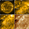 |
Fig. 1. Overview of the observations. Panel (A): Full disk image of the solar corona as observed with 171 Å filter of the SDO/AIA. Panel (B): Part of the field of view of the HRIEUV that shows active region loops. This field of view is outlined by the white box in panel (A). Panels (C) and (D): Roughly the same region as seen by the AIA 171 Å and 193 Å filters, respectively. The white dotted lines trace the three loops described in the text. The intensity in panel (A) is displayed in square root scale. Panels (B)–(D) are time averages of three images for each passband that are closest in time with the image shown in panel (A) and are plotted in log scale. |
The corresponding AIA data were respiked using the SolarSoft procedure aia_respike. We used aia_prep to eliminate the spacecraft roll angle, update the pointing information, and set the plate scale to 0.6″ per pixel. Additionally, we registered the entire AIA data set with the first AIA image to remove the solar rotation using coreg_map. We utilized a subset of the HRIEUV data set with a cadence of 10 s spanning from 03:25:49 to 04:25:49 UT because it closely matches the 12 s cadence of the SDO/AIA filters.
To align the AIA data with the HRIEUV images, we extracted World Coordinate System (WCS; Thompson 2006) information from the EUI header files and calculated the Carrington coordinates using the IDL routine wcs_convert_from_coord. Using wcs_convert_to_coord, we then calculated the corresponding world coordinates in AIA passbands. To refine alignment, manual adjustments were made by tracking common features in the HRIEUV images and the AIA 171 Å passband.
Figure 1 provides a comprehensive view of the region of interest (ROI). We focus on the bright closed loops with relatively low backgrounds in the AR. At the time of observation, the angle between the Solar Orbiter and the Sun–Earth line is ∼43°, resulting in the foreshortening of these loops in the AIA images. Despite this distortion, we were able to visually identify ten prominent loops consistent across the two instruments, based on their footpoints and similar morphology.
The HRIEUV instrument on board Solar Orbiter samples the plasma at ∼1 MK; Fe IX and Fe X are the dominant species that contribute to the emission detected by the passband. The AIA 171 Å filter captures the plasma at ∼0.8 MK primarily dominated by Fe IX ions. This overlap in temperature response functions coupled with the inherent multi-thermal structure of the coronal loops causes them to exhibit similar temporal evolutions when observed with these two instruments. This similarity aids in identifying the same loops in data sets obtained from two vantage points making them ideal for stereoscopic studies of coronal loops. Additionally, the AIA 193 Å channel is dominated by Fe XII ions in quiet-Sun and nonflaring ARs, and samples the plasma at ∼1.5 MK. This difference in temperature response between the AIA 193 Å, and the cooler AIA 171 Å filter and the HRIEUV offers possibility to investigate multi-thermal evolution of loops, providing a more comprehensive view of their dynamics.
3. Results
3.1. Similar temporal evolution of loops from two vantage points
Following the visual identification of each loop, we then compared their temporal evolution across both instruments using light curves. These light curves were generated by averaging the intensity within ∼2.2 × 2.2 Mm boxes (20 × 20 pixel in HRIEUV and 5 × 5 pixel in AIA) positioned on the loop axes. Notably, these boxes are not remapped between the HRIEUV and AIA instruments. We manually position the boxes in both data sets on loop segments with darker backgrounds. The HRIEUV box position was fixed initially, while the box in AIA 171 Å filter was incrementally moved along the loop within the low-background segment. If the light curves from these boxes displayed similar intensity variations, then the HRIEUV box position was slightly shifted along the loop length and the process was repeated. This ensured that the temporal evolution of the entire HRIEUV loop segment with a low background matched the corresponding segment in the AIA 171 Å filter.
We also compared the light curves of neighboring loops in the AIA 171 Å passband with the identified loop in the HRIEUV data. We found that adjacent loops exhibited noticeably different temporal variations on longer timescales (see Appendix A). Therefore, it further ensured that we are identifying the same loop in the AIA 171 Å filter and are not confusing it with an adjacent loop. The shorter observation period, which spans ∼1 hr, minimizes significant movements of the loops in the plane of the sky. We also reviewed the accompanying movies to ensure that the light curves are unaffected by loops moving out of the boxes. Though rare, if this movement occurs, the box placement is adjusted accordingly. We performed this analysis on ten visually identified loops. Three such loops are highlighted in panels (B)–(D) of Fig. 1.
Figure 2 illustrates the evolution of loop 1 located in the core of the AR. The accompanied animation shows that the loop is distinctly visible in the AIA 171 Å filter and HRIEUV images, with a faint presence in the AIA 193 Å passband at the beginning of the observations. Subsequently, the loop becomes fainter across all three channels, but it almost fades away in the AIA 193 Å filter (03:48 – 03:56 UT, see Fig. 2D and accompanying animation). Later, a resurgence occurs, and the loop becomes bright in all three channels almost simultaneously in the AIA 171 Å passband and HRIEUV images (04:00 UT), followed slightly later by the AIA 193 Å passband (04:11 UT). This brightening is transient, as the loop once again becomes faint across all three channels almost concurrently. This recurring trend is evident in panel (D) of Fig. 2 where we show the light curves for the loop apex.
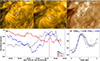 |
Fig. 2. Evolution of loop 1. Panels (A)–(C) show the snapshots of loop 1 in the AIA 171 Å, HRIEUV, and AIA 193 Å passbands, respectively. The arrows highlight the color-coded boxes spanning 5 × 5 pixel in both of the AIA passbands and 20 × 20 pixel in the EUI 174 Å passband. The average intensities within these boxes are utilized to compute the light curves, which are subsequently normalized by their individual maximum values. These normalized light curves are plotted in panel (D) using the same colors as their corresponding boxes. The color-coded solid lines near the boxes in panels (A) and (B) represent roughly 1.3 Mm wide artificial slits that we used to calculate the loop widths in panel (E). The lengths of these slits differ for different loops depending upon the loop width and the presence of adjacent loops. The data points in panel (E) correspond to the average intensities observed along the artificial transverse slits, and the solid lines show their respective Gaussian fits. The intensities in panel (E) are normalized with the respective maxima. The error bars show 1σ uncertainties in the measurements due to the Poisson errors that arise from photon noise. Panels (A)–(C) are plotted in log scale. An animation of panels (A)–(D) is available online. |
This trend is noticeable not only within the AR core, but also in the loops extending beyond it. Figure 3 focuses on a loop consisting of multiple strands. These strands originate in the periphery of the AR core and extend to another footpoint that is not not apparent, but seems to be somewhere near the core. Panel (D) of this figure demonstrates the similar evolution of one of these strands observed in the HRIEUV and the AIA 171 Å passband. Initially, during the start of the observations, the strand is distinctly visible within the loop in the HRIEUV and the AIA 171 Å channels; however, it appears fuzzy, but still distinguishable in the AIA 193 Å images. As the evolution progresses the loop fades away in the HRIEUV and the AIA 171 Å passband (at around 03:46 UT; see Fig. 3D and accompanying animation), while it becomes more distinct and luminous in the AIA 193 Å channel (around 04:00 UT). By the end, it becomes distinctly visible in both the HRIEUV images and the AIA 171 Å filter; however, the entire loop becomes fuzzy in AIA 193 Å. It suggests that this loop is also showing nearly identical evolution across the HRIEUV and the AIA 171 Å filter.
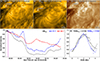 |
Fig. 3. Evolution of loop 2. The panel layout, box sizes for light curves, and slit width are the same as for Fig. 2. An animation of panels (A)–(D) is available online. |
This analysis reveals that the identified loops exhibit intensity variations predominantly on two distinct timescales: a shorter scale of 5–10 minutes and a longer scale of 20–30 minutes. We find that the evolution of these loops does not appear to correlate on shorter timescales. However, we observe very similar evolution patterns between the HRIEUV images and AIA 171 Å passband on longer timescales. Most of these loops appear fuzzy in the AIA 193 Å passband, and their light curves exhibit noticeably different evolution patterns compared to the HRIEUV and AIA 171 Å light curves on both shorter and longer timescales.
3.2. Loop widths
Furthermore, we compared the widths of these loops as observed in the HRIEUV images and the AIA 171 Å passband (see panel (E) of Figs. 2 and 3, and panels (1–9) of Fig. 4). To calculate the widths, we placed a ∼1.5 Mm wide slit across the length of the loop near the points where the loop displays a coherent evolution across these instruments. The average intensity profile (for three consecutive frames) along the slit is then fitted with a single Gaussian model with five free parameters, including a constant term and a linear trend. The FWHM derived from these fits serves as a measure of the loop cross-sectional widths. The loops in our observations exhibit widths in the range of 0.56 ± 0.15 Mm to 3.76 ± 0.01 Mm. Notably, some loops in the HRIEUV images exhibit substructure, with strands appearing as multiple peaks in the intensity profiles used for these Gaussian fits. However, in most cases, the AIA 171 Å counterparts lacked the spatial resolution to resolve these individual strands. For instance, loop 1 displays two strands in the HRIEUV images which are evident due to a small intensity dip in the middle of the profile (black curve in panel (E) of Fig. 2). In contrast, the AIA 171 Å curve does not resolve these individual strands, necessitating the use of a single-peaked Gaussian function for width measurement. Additionally, the width of loop 8 in Fig. 4 was measured to be 2.97 Mm in AIA 171 Å, due to the bright background moss region artificially making the loop appear thicker. Nevertheless, we identified a similarity in widths between the HRIEUV images and the AIA 171 Å passband, with the largest difference (excluding loop 8) being 1.3 Mm.
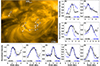 |
Fig. 4. Comparison of loop widths from two vantage points. For visualization purposes, we selected a single HRIEUV snapshot for each loop at its peak brightness. The top left panel displays the average of these nine snapshots. The black lines indicate slit positions used for width calculations in the HRIEUV data. Panels (1)–(9) plot the intensity profiles for the individual loops (numbered 1–9) corresponding to the positions in the top left panel. Measurements in black (HRIEUV) and blue (AIA 171 Å) represent the loop widths as described in the caption of Fig. 2E. These loop widths are tabulated in Appendix D.1 |
3.3. Coherency
The entire loop 3 is distinctly visible throughout the observational period in HRIEUV images. This visibility facilitates a detailed comparison with other segments of the same loop that lack the underlying moss emission. Figure 5 illustrates the intensity variation for three such segments of this loop. The average intensity inside all three boxes displays a rise phase, a plateau, and then a gradual decrease. Although the intensity variations across the three segments do not correlate well over shorter timescales, there is a clear similarity in their long-term variations. This indicates a coherent thermal evolution along the length of the loop. Interestingly, a segment of this loop near the west footpoint does not show a clear temporal coherence between the HRIEUV and AIA 171 Å filter (see Appendix B). A prominent peak seen in the three moss-free segments around 03:40 – 04:00 UT is also faintly present in this loop segment (indicated by black arrows in Figs. B.1D and 5B). However, these three loop segments do not exhibit enhanced brightening toward the end of the observational period, unlike the loop segment with moss in Fig. B.1. We also include the intensity variation of a segment of loop 3 that is outside of the moss region, as seen by the AIA 171 Å filter, as a magenta curve. We find that it also displays a prominent peak at ∼03:50 UT and no noticeable brightening by the end of the observation period. This is in line with the HRIEUV segments that lack the moss emission in the background. This emphasizes the consistency observed in segments that are minimally affected by the background moss emission, indicating similar behavior between the HRIEUV and AIA 171 Å data.
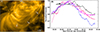 |
Fig. 5. Coherent evolution of a loop. Panel (A) shows a one-hour time average of HRIEUV images, starting at 03:23:49 UT on 07 April 2023. Three arrows point to 15 × 15 pixel color-coded boxes representing different segments of loop 3 (see Fig. 1). Panel (B) displays colored light curves for these boxes, calculated using the process outlined in the caption of Fig. 2. The black arrow highlights the intensity enhancement exhibited by all the loop segments at around 03:40 UT. The image in panel (A) is plotted in log scale. |
4. Discussion
Accurately matching corresponding loop segments between different vantage points can be challenging. Malanushenko & Schrijver (2013) pointed out that the presence of multiple loops with elongated cross sections in close proximity can lead to false identifications, due to the potential overlap or resemblance among adjacent loops. Our analysis reveals that the identified loops predominantly exhibit intensity variations on two distinct timescales. The short-term oscillations, in the 5–10 min range, are associated with the background moss regions and can be linked to p-mode oscillations (Brynildsen et al. 2003; Marsh & Walsh 2006). On a longer timescale of 20–30 minutes, we observe consistent intensity variations across the instruments. These longer timescale oscillations are typically associated with the cooling times of coronal loops. Consequently, if instruments observe plasma at similar temperatures, a coronal loop with a 3D structure is expected to display a similar evolution pattern from two vantage points. Notably, these observations are taken at a separation angle of approximately 43°, implying that the background and foreground features differ significantly for observations from each instrument. Nevertheless, we investigated whether the background could influence the light curves used to compare the thermal evolution of these loops across instruments. Our findings demonstrate that as long as the background is sufficiently dark, it does not substantially affect the observed intensity variations (see Appendix C) and aligns with the results from López Fuentes et al. (2008) on TRACE loops. Therefore, the similarity in emission patterns from two vantage points is unlikely to originate from features other than loops. Additionally, the neighboring loops show different emission patterns in the light curves. This further highlights the reliability of our analysis.
4.1. Spatio-temporal morphology of coronal loops
We proceeded to measure the widths of these loops as observed from both vantage points. The widths of the loops included in this study range between 0.67 and 3.76 Mm, consistent with the findings from previous studies of EUV loops (Patsourakos & Klimchuk 2007; Aschwanden et al. 2008; Aschwanden & Peter 2017). We observed that these loops generally have similar widths across the instruments, with the largest difference being 1.3 Mm. This suggests that these loops have nearly circular cross sections, as recently found by Mandal et al. (2024). The thinnest loop included in this study has a width of 660 km in the HRIEUV images. Conversely, the Gaussian profile of the AIA counterpart of this loop has a width of 2.97 Mm. This discrepancy is likely attributable to the bright background that may artificially render these loops thicker. Additionally, Peter et al. (2013) identified miniature loops in Hi-C observations as short as 1 Mm and approximately 200 km wide. However, they did not find any evidence of substructure in the larger loops at scales of 0.1″ pixel−1. They estimated that for these loops to be multi-stranded without showing substructure, the individual strands would need to be narrower than 15 km.
The consistency in intensity variations and widths of the loops observed from two different vantage points implies that the emission likely emanates from 3D structures rather than flat sheet-like structures aligned along the LOS, as suggested by Malanushenko et al. (2022). Our observation of a coherent thermal evolution along the entire length of an individual loop, based on stereoscopic analysis, further supports this finding. This coherence indicates that the emission originates from a 3D structure with a heating mechanism that elicits a global response across the loop. Such a structure could be composed of thin unresolved strands. Alternatively, a substructure of a loop might arise from the emission from overlapping contributions of numerous randomly oriented wrinkles within a single 2D plasma sheet. While this scenario might create an impression of a 3D structure, it would require these tiny veils to be confined within a highly unlikely circular envelope. Furthermore, even under such conditions, it is unlikely that this arrangement could consistently produce similar intensity variations when observed from two viewing angles separated by 43°, as the emission from the second perspective would come from different segments of these wrinkles. Uritsky & Klimchuk (2024) investigated the influence of projection effects on 3D structures with varying cross sections and two-dimensional (2D) plasma sheets in an optically thin corona. They suggested that most EUV coronal loops are 3D tube-like structures and are not likely to be projections of 2D sheets. The coherency is not only imprinted in the thermal evolution as shown in this study, but also in the signatures of decayless kink oscillations of coronal loops as recently inferred using coronal observations from two vantage points (Zhong et al. 2023).
4.2. Nature of coronal loop heating
The observed loops could be heated by storms of nanoflares events (Klimchuk et al. 2023), facilitated by untangling of small-scale magnetic braids in the corona (Chitta et al. 2022). Further observations are needed to determine the specific distribution of nanoflares within these structures. One key question is whether these nanoflare storms are localized at a single point of the loop or are distributed throughout its entire length. In either case, thermal conduction would rapidly distribute the heat, leading to a consistent intensity evolution pattern along the length. If the storms are distributed along the length of the loop, then what triggers their simultaneous occurrence remains an open question. Simulations do show that a single unstable strand experiencing kink instability can trigger an avalanche, thus disrupting neighboring strands (Hood et al. 2016). Reid et al. (2020) demonstrate that the kink instability heats the first strand primarily through strong bursts of Ohmic heating. As the cascade progresses, viscous heating becomes dominant, occurring in a large number of small heating events. They find that there is no clear preferred location for heating within the loop, and the heating events are spread throughout the inner 90% of the loop length.
With the spatio-temporal coherence of loop emission presented here, our study tends to support the conclusions from the MHD simulations. However, a more quantitative comparison of emission patterns of simulated loops (both spatial and temporal) with the type of observations we presented here is required to fully comprehend the spatial distribution of heating events in coronal loops. For instance, high-resolution MHD simulations that use self-consistent convective driving to heat coronal loop plasma (Breu et al. 2022) will be useful for such a comparison. The slow footpoint driving leads to the development of turbulence in the coronal section of the loop in these simulations. This turbulence may, on the one hand, lead to a uniform distribution of heating events, and on the other hand, smooth out the current sheets to form coherent strand-like or loop-like features.
4.3. Line-of-sight effects
We note that the possibility of some coronal loops being projection effects of 2D plasma sheets cannot be completely ruled out with the current observations as the widths measured in this study may not fully account for the true cross-sectional shapes of the loops. If these loops were indeed 2D sheets, their apparent widths would vary depending on the angle between the LOS and the plane of the sheet. For example, if the LOS were parallel to the plane of a light emitting sheet, then it would appear to have its actual width, while it would be invisible if the LOS were perpendicular to the plane of the sheet. Intermediate angles cause the sheet to appear narrower, resembling loops with varied widths depending on different vantage points. To disentangle these effects, observations from a second vantage point from outside the ecliptic plane could be helpful. By viewing the structure from multiple planes, it would be possible to measure its actual width and determine its three-dimensional structure more accurately.
Practically, however, a north–south aligned coronal loop seen from different viewing angles from the same plane might also help in resolving the ambiguity between 2D sheet and 3D tube morphology. In our observations, there are indeed loop segments that are aligned nearly in the north–south orientation (e.g., the case presented in Fig. B.1). The loop segment indicates more of a 3D tube-like morphology instead of a 2D sheet-like feature. Therefore, we tend to agree with the suggestion that the observed loops are 3D features rather than projections of randomly aligned wrinkles in 2D plasma sheets.
5. Conclusions
We analyzed AR coronal loops from two vantage points using the Solar Orbiter and Solar Dynamics Observatory, with a separation angle of ∼43° between their LOSs. This approach may provide insights into their three-dimensional geometry, including cross sections and coherent thermal evolution. These coronal loops appear foreshortened in the AIA images since the ROI is close to the limb. Nevertheless, we were able to identify ten distinct loops that were relatively isolated and present across both instruments, the HRIEUV and in the AIA 171 Å passband. The identified loops were scattered throughout the AR, with some located close to the core and others near the boundaries. After accounting for the possible contamination from the background features, our analysis suggests that the coronal loops show similar evolution of emission patterns from two different vantage points and along their lengths on timescales of about 30 minutes. The similar intensity variation across the instruments shows that we are indeed observing the same segment of a coherent 3D structure in the solar corona. We also find that these loops have similar widths across the two instruments, which suggests that they have nearly circular cross sections. These results hint that coronal loops are unlikely to be imprints of LOS-integrated emission from a distribution of 2D veil-like structures.
Data availability
Movies associated to Figs. 2, 3, and B.1 are available at https://www.aanda.org
Acknowledgments
We thank the anonymous referee for their helpful comments that improved the presentation of the manuscript. B.R. and L.P.C. gratefully acknowledge funding by the European Union (ERC, ORIGIN, 101039844). Views and opinions expressed are however those of the author(s) only and do not necessarily reflect those of the European Union or the European Research Council. Neither the European Union nor the granting authority can be held responsible for them. The work of S.M. has been supported by Deutsches Zentrum für Luft- und Raumfahrt (DLR) through grant DLR_FKZ 50OU2201. Solar Orbiter is a space mission of international collaboration between ESA and NASA, operated by ESA. We thank the ESA SOC and MOC teams for their support. The EUI instrument was built by CSL, IAS, MPS, MSSL/UCL, PMOD/WRC, ROB, LCF/IO with funding from the Belgian Federal Science Policy Office (BELSPO/PRODEX PEA 4000106864 and 4000112292); the Centre National d’ Etudes Spatiales (CNES); the UK Space Agency (UKSA); the Bundesministerium für Wirtschaft und Energie (BMWi) through the Deutsches Zentrum für Luft- und Raumfahrt (DLR); and the Swiss Space Office (SSO). SDO is the first mission to be launched for NASA’s Living With a Star (LWS) Program and the data supplied courtesy of the HMI and AIA consortia. This research has made use of NASA’s Astrophysics Data System Bibliographic Services.
References
- Amari, T., & Luciani, J. F. 1999, ApJ, 515, L81 [NASA ADS] [CrossRef] [Google Scholar]
- Aschwanden, M. J. 2002, in SOLMAG 2002. Proceedings of the Magnetic Coupling of the Solar Atmosphere Euroconference, ed. H. Sawaya-Lacoste, ESA Spec. Publ., 505, 191 [NASA ADS] [Google Scholar]
- Aschwanden, M. J., & Peter, H. 2017, ApJ, 840, 4 [CrossRef] [Google Scholar]
- Aschwanden, M. J., Wülser, J.-P., Nitta, N. V., & Lemen, J. R. 2008, ApJ, 679, 827 [NASA ADS] [CrossRef] [Google Scholar]
- Asgari-Targhi, M., Schmelz, J. T., Imada, S., Pathak, S., & Christian, G. M. 2015, ApJ, 807, 146 [NASA ADS] [CrossRef] [Google Scholar]
- Breu, C., Peter, H., Cameron, R., et al. 2022, A&A, 658, A45 [NASA ADS] [CrossRef] [EDP Sciences] [Google Scholar]
- Brynildsen, N., Maltby, P., Kjeldseth-Moe, O., & Wilhelm, K. 2003, A&A, 398, L15 [NASA ADS] [CrossRef] [EDP Sciences] [Google Scholar]
- Cargill, P. J., & Klimchuk, J. A. 2004, ApJ, 605, 911 [NASA ADS] [CrossRef] [Google Scholar]
- Chitta, L. P., Peter, H., Parenti, S., et al. 2022, A&A, 667, A166 (SO Nominal Mission Phase SI) [NASA ADS] [CrossRef] [EDP Sciences] [Google Scholar]
- Culhane, J. L., Harra, L. K., James, A. M., et al. 2007, Sol. Phys., 243, 19 [Google Scholar]
- Di Matteo, V., Reale, F., Peres, G., & Golub, L. 1999, A&A, 342, 563 [NASA ADS] [Google Scholar]
- Gudiksen, B. V., & Nordlund, Å. 2005, ApJ, 618, 1031 [Google Scholar]
- Handy, B. N., Acton, L. W., Kankelborg, C. C., et al. 1999, Sol. Phys., 187, 229 [Google Scholar]
- Hollweg, J. V. 1981, Sol. Phys., 70, 25 [Google Scholar]
- Hood, A. W., Cargill, P. J., Browning, P. K., & Tam, K. V. 2016, ApJ, 817, 5 [NASA ADS] [CrossRef] [Google Scholar]
- Klimchuk, J. A. 2000, Sol. Phys., 193, 53 [NASA ADS] [CrossRef] [Google Scholar]
- Klimchuk, J. A. 2006, Sol. Phys., 234, 41 [Google Scholar]
- Klimchuk, J. A., & DeForest, C. E. 2020, ApJ, 900, 167 [NASA ADS] [CrossRef] [Google Scholar]
- Klimchuk, J. A., Lemen, J. R., Feldman, U., Tsuneta, S., & Uchida, Y. 1992, PASJ, 44, L181 [NASA ADS] [CrossRef] [Google Scholar]
- Klimchuk, J. A., Knizhnik, K. J., & Uritsky, V. M. 2023, ApJ, 942, 10 [NASA ADS] [CrossRef] [Google Scholar]
- Kobayashi, K., Cirtain, J., Winebarger, A. R., et al. 2014, Sol. Phys., 289, 4393 [Google Scholar]
- Kosugi, T., Matsuzaki, K., Sakao, T., et al. 2007, Sol. Phys., 243, 3 [Google Scholar]
- Kraaikamp, E., Gissot, S., Stegen, K., et al. 2023, SolO/EUI Data Release 6.0 (Royal Observatory of Belgium, ROB) [Google Scholar]
- Kucera, T. A., Young, P. R., Klimchuk, J. A., & DeForest, C. E. 2019, ApJ, 885, 7 [NASA ADS] [CrossRef] [Google Scholar]
- Lemen, J. R., Title, A. M., Akin, D. J., et al. 2012, Sol. Phys., 275, 17 [Google Scholar]
- López Fuentes, M. C., & Klimchuk, J. A. 2010, ApJ, 719, 591 [CrossRef] [Google Scholar]
- López Fuentes, M. C., Klimchuk, J. A., & Démoulin, P. 2006, ApJ, 639, 459 [CrossRef] [Google Scholar]
- López Fuentes, M. C., Klimchuk, J. A., & Mandrini, C. H. 2007, ApJ, 657, 1127 [CrossRef] [Google Scholar]
- López Fuentes, M. C., Démoulin, P., & Klimchuk, J. A. 2008, ApJ, 673, 586 [CrossRef] [Google Scholar]
- Malanushenko, A., & Schrijver, C. J. 2013, ApJ, 775, 120 [NASA ADS] [CrossRef] [Google Scholar]
- Malanushenko, A., Cheung, M. C. M., DeForest, C. E., Klimchuk, J. A., & Rempel, M. 2022, ApJ, 927, 1 [NASA ADS] [CrossRef] [Google Scholar]
- Mandal, S., Peter, H., Klimchuk, J. A., et al. 2024, A&A, 682, L9 (SO Nominal Mission Phase SI) [NASA ADS] [CrossRef] [EDP Sciences] [Google Scholar]
- Marsh, M. S., & Walsh, R. W. 2006, ApJ, 643, 540 [NASA ADS] [CrossRef] [Google Scholar]
- McIntosh, S. W., de Pontieu, B., Carlsson, M., et al. 2011, Nature, 475, 477 [Google Scholar]
- Müller, D., StCyr, O. C., Zouganelis, I., et al. 2020, A&A, 642, A1 [NASA ADS] [CrossRef] [EDP Sciences] [Google Scholar]
- Parker, E. N. 1988, ApJ, 330, 474 [Google Scholar]
- Patsourakos, S., & Klimchuk, J. A. 2007, ApJ, 667, 591 [NASA ADS] [CrossRef] [Google Scholar]
- Pesnell, W. D., Thompson, B. J., & Chamberlin, P. C. 2012, Sol. Phys., 275, 3 [Google Scholar]
- Peter, H., & Bingert, S. 2012, A&A, 548, A1 [NASA ADS] [CrossRef] [EDP Sciences] [Google Scholar]
- Peter, H., Bingert, S., Klimchuk, J. A., et al. 2013, A&A, 556, A104 [NASA ADS] [CrossRef] [EDP Sciences] [Google Scholar]
- Plowman, J. E., Kankelborg, C. C., & Longcope, D. W. 2009, ApJ, 706, 108 [NASA ADS] [CrossRef] [Google Scholar]
- Reale, F. 2014, Liv. Rev. Sol. Phys., 11, 4 [Google Scholar]
- Reid, J., Cargill, P. J., Hood, A. W., Parnell, C. E., & Arber, T. D. 2020, A&A, 633, A158 [NASA ADS] [CrossRef] [EDP Sciences] [Google Scholar]
- Rochus, P., Auchère, F., Berghmans, D., et al. 2020, A&A, 642, A8 [NASA ADS] [CrossRef] [EDP Sciences] [Google Scholar]
- Testa, P., Peres, G., Reale, F., & Orlando, S. 2002, ApJ, 580, 1159 [NASA ADS] [CrossRef] [Google Scholar]
- Thompson, W. T. 2006, A&A, 449, 791 [NASA ADS] [CrossRef] [EDP Sciences] [Google Scholar]
- Uritsky, V. M., & Klimchuk, J. A. 2024, ApJ, 961, 222 [NASA ADS] [CrossRef] [Google Scholar]
- Van Doorsselaere, T., Srivastava, A. K., Antolin, P., et al. 2020, Space Sci. Rev., 216, 140 [Google Scholar]
- Viall, N. M., & Klimchuk, J. A. 2012, ApJ, 753, 35 [CrossRef] [Google Scholar]
- Walsh, R. W., & Ireland, J. 2003, A&ARv, 12, 1 [CrossRef] [Google Scholar]
- Wang, H., & Sakurai, T. 1998, PASJ, 50, 111 [NASA ADS] [CrossRef] [Google Scholar]
- Warren, H. P., Winebarger, A. R., & Mariska, J. T. 2003, ApJ, 593, 1174 [NASA ADS] [CrossRef] [Google Scholar]
- Watko, J. A., & Klimchuk, J. A. 2000, Sol. Phys., 193, 77 [NASA ADS] [CrossRef] [Google Scholar]
- Winebarger, A. R., & Warren, H. P. 2005, ApJ, 626, 543 [NASA ADS] [CrossRef] [Google Scholar]
- Winebarger, A. R., Warren, H. P., & Seaton, D. B. 2003, ApJ, 593, 1164 [NASA ADS] [CrossRef] [Google Scholar]
- Withbroe, G. L., & Noyes, R. W. 1977, ARA&A, 15, 363 [Google Scholar]
- Zhong, S., Nakariakov, V. M., Kolotkov, D. Y., et al. 2023, Nat. Commun., 14, 5298 [NASA ADS] [CrossRef] [Google Scholar]
Appendix A: Comparison of the intensity pattern of two adjacent loops
The light curves from adjacent loops exhibit noticeably different emission patterns. Figure A.1 displays the time evolution of loop 1 and loop 4 (see also Fig. 4). Initially, the light curves from loop 1 (black and blue) show a decrease in intensity in both instruments. This intensity dip around 4:52 UT is followed by an increase, with the peak appearing slightly later in AIA 171Å. This delay is likely due to the AIA 171 Å filter being more sensitive to slightly cooler temperatures than HRIEUV. In contrast, the light curves of loop 4 (green and red) exhibit a steady increase in intensity throughout the observation period.
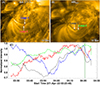 |
Fig. A.1. Difference in the evolution patterns of adjacent loops. Panels (A) and (B) showcase snapshots of the AIA 171 Å and HRIEUV passbands, respectively, at 04:21:09 UT. Panel (C) shows the color-coded light curves for the boxes marked in panels (A) and (B). Procedure to calculate light curve is described in the caption of Fig. 2. The box size for loop 1 in AIA and HRIEUV are increased to 9 × 9 and 36 × 36 pixel, respectively. |
Appendix B: Dissimilar temporal evolution of a loop from two vantage points
We also find a case where the loop shows a similar overarching trend in both HRIEUV and AIA 171 Å filter but notable dissimilarities emerge within the evolutionary pattern. Figure B.1 displays the evolution of loop 3 close to its footpoint. Light curves in Panel (D) showcase that the overall normalized intensity is increasing throughout the observational period in both instruments. However, two prominent intensity peaks in the HRIEUV light curves (the left peak is highlighted by a black arrow) are absent in both AIA filters. The presence of a bright moss region in the background is a potential contributor to these discrepancies. This background emission, integrated along the LOS, could potentially influence the observed intensity.
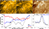 |
Fig. B.1. Evolution of loop 3. The panel layout, color, and size of the boxes for the light curves, and the slit widths are similar to those in Fig. 2. The average intensity within the 5 × 5 pixel magenta box in panel (A) is used to derive the correspondingly colored light curve in panel (B) of Fig. 5. The black arrow points to the intensity enhancement in the HRIEUV light curve. An animation of panels (A)-(D) is available online. |
Appendix C: Influence of background emission
To analyze the influence of background emission on the light curves from the loops or strands, we examine the intensity variations in regions adjacent to loop 3, as illustrated in Fig. C.1. We position additional boxes on the northern and southern sides of those boxes used for plotting the light curves in Fig. 5. In these new light curves, absolute intensity is plotted instead of normalized intensity. Upon examination, the blue box in segment (a) of this loop displays an evolution very similar to the box on the loop axis (black box). This similarity may be attributed to the blue box encompassing other strands of the same loop. In contrast, the red box in this segment corresponds to a low-background region and exhibits significantly lower brightness. However, it does show intensity patterns that are somewhat similar to those of the blue and black boxes, albeit at lower intensities. Light curves generated for segments (b) and (c), in comparison to their surrounding background emission, exhibit dissimilar behavior. Therefore, our analysis suggests that the integration of background emission in the loop segments, particularly where the background is not very bright, does not significantly influence the resulting light curves.
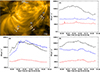 |
Fig. C.1. Influence of the background emission. The top left panel shows a one-hour time average of HRIEUV images, starting at 03:23:49 UT on 07 April 2023. In the top left panel, (a), (b), and (c) denote the three loop segments for which the light curves are plotted in panels (a) - (c) respectively. White arrows indicate the color-coded boxes for which light curves are plotted in the subsequent panels. |
Appendix D: Loop widths
Comparison of Loop Widths
All Tables
All Figures
|
Fig. 1. Overview of the observations. Panel (A): Full disk image of the solar corona as observed with 171 Å filter of the SDO/AIA. Panel (B): Part of the field of view of the HRIEUV that shows active region loops. This field of view is outlined by the white box in panel (A). Panels (C) and (D): Roughly the same region as seen by the AIA 171 Å and 193 Å filters, respectively. The white dotted lines trace the three loops described in the text. The intensity in panel (A) is displayed in square root scale. Panels (B)–(D) are time averages of three images for each passband that are closest in time with the image shown in panel (A) and are plotted in log scale. |
| In the text | |
|
Fig. 2. Evolution of loop 1. Panels (A)–(C) show the snapshots of loop 1 in the AIA 171 Å, HRIEUV, and AIA 193 Å passbands, respectively. The arrows highlight the color-coded boxes spanning 5 × 5 pixel in both of the AIA passbands and 20 × 20 pixel in the EUI 174 Å passband. The average intensities within these boxes are utilized to compute the light curves, which are subsequently normalized by their individual maximum values. These normalized light curves are plotted in panel (D) using the same colors as their corresponding boxes. The color-coded solid lines near the boxes in panels (A) and (B) represent roughly 1.3 Mm wide artificial slits that we used to calculate the loop widths in panel (E). The lengths of these slits differ for different loops depending upon the loop width and the presence of adjacent loops. The data points in panel (E) correspond to the average intensities observed along the artificial transverse slits, and the solid lines show their respective Gaussian fits. The intensities in panel (E) are normalized with the respective maxima. The error bars show 1σ uncertainties in the measurements due to the Poisson errors that arise from photon noise. Panels (A)–(C) are plotted in log scale. An animation of panels (A)–(D) is available online. |
| In the text | |
|
Fig. 3. Evolution of loop 2. The panel layout, box sizes for light curves, and slit width are the same as for Fig. 2. An animation of panels (A)–(D) is available online. |
| In the text | |
|
Fig. 4. Comparison of loop widths from two vantage points. For visualization purposes, we selected a single HRIEUV snapshot for each loop at its peak brightness. The top left panel displays the average of these nine snapshots. The black lines indicate slit positions used for width calculations in the HRIEUV data. Panels (1)–(9) plot the intensity profiles for the individual loops (numbered 1–9) corresponding to the positions in the top left panel. Measurements in black (HRIEUV) and blue (AIA 171 Å) represent the loop widths as described in the caption of Fig. 2E. These loop widths are tabulated in Appendix D.1 |
| In the text | |
|
Fig. 5. Coherent evolution of a loop. Panel (A) shows a one-hour time average of HRIEUV images, starting at 03:23:49 UT on 07 April 2023. Three arrows point to 15 × 15 pixel color-coded boxes representing different segments of loop 3 (see Fig. 1). Panel (B) displays colored light curves for these boxes, calculated using the process outlined in the caption of Fig. 2. The black arrow highlights the intensity enhancement exhibited by all the loop segments at around 03:40 UT. The image in panel (A) is plotted in log scale. |
| In the text | |
|
Fig. A.1. Difference in the evolution patterns of adjacent loops. Panels (A) and (B) showcase snapshots of the AIA 171 Å and HRIEUV passbands, respectively, at 04:21:09 UT. Panel (C) shows the color-coded light curves for the boxes marked in panels (A) and (B). Procedure to calculate light curve is described in the caption of Fig. 2. The box size for loop 1 in AIA and HRIEUV are increased to 9 × 9 and 36 × 36 pixel, respectively. |
| In the text | |
|
Fig. B.1. Evolution of loop 3. The panel layout, color, and size of the boxes for the light curves, and the slit widths are similar to those in Fig. 2. The average intensity within the 5 × 5 pixel magenta box in panel (A) is used to derive the correspondingly colored light curve in panel (B) of Fig. 5. The black arrow points to the intensity enhancement in the HRIEUV light curve. An animation of panels (A)-(D) is available online. |
| In the text | |
|
Fig. C.1. Influence of the background emission. The top left panel shows a one-hour time average of HRIEUV images, starting at 03:23:49 UT on 07 April 2023. In the top left panel, (a), (b), and (c) denote the three loop segments for which the light curves are plotted in panels (a) - (c) respectively. White arrows indicate the color-coded boxes for which light curves are plotted in the subsequent panels. |
| In the text | |
Current usage metrics show cumulative count of Article Views (full-text article views including HTML views, PDF and ePub downloads, according to the available data) and Abstracts Views on Vision4Press platform.
Data correspond to usage on the plateform after 2015. The current usage metrics is available 48-96 hours after online publication and is updated daily on week days.
Initial download of the metrics may take a while.