| Issue |
A&A
Volume 697, May 2025
|
|
|---|---|---|
| Article Number | A233 | |
| Number of page(s) | 9 | |
| Section | The Sun and the Heliosphere | |
| DOI | https://doi.org/10.1051/0004-6361/202553934 | |
| Published online | 22 May 2025 | |
Anomalous cross-field motions of solar coronal loops
1
Max Planck Institute for Solar System Research, Justus-von-Liebig-Weg 3, 37077 Göttingen, Germany
2
Institut für Sonnenphysik (KIS), Georges-Köhler-Allee 401a, 79110 Freiburg, Germany
3
NASA Goddard Space Flight Center, Greenbelt, Maryland, USA
⋆ Corresponding author: This email address is being protected from spambots. You need JavaScript enabled to view it.
Received:
28
January
2025
Accepted:
2
April
2025
Abstract
We present several examples of unusual evolutionary patterns in solar coronal loops that resemble cross-field drift motions. These loops were simultaneously observed from two vantage points by two different spacecraft: the High-Resolution Imager of the Extreme Ultraviolet Imager aboard the Solar Orbiter and the Atmospheric Imaging Assembly aboard the Solar Dynamics Observatory. Across all these events, a recurring pattern is observed: Initially, a thin, strand-like structure detaches and shifts several megameters away from a main or parent loop. During this period, the parent loop remains intact in its original position. After a few minutes, the shifted strand reverses its direction and returns to the location of the parent loop. Key features of this “split-drift” type evolution are: (i) the presence of kink oscillations in the loops before and after the split events and (ii) a sudden split motion at about 30 km s−1, with additional slow drifts, either away from or back to the parent loops, at around 5 km s−1. Co-temporal photospheric magnetic field data obtained from the Helioseismic and Magnetic Imager reveal that during such split-drift evolution, one of the loop points in the photosphere moves back and forth between nearby magnetic polarities. While the exact cause of this split drift phenomenon is still unclear, the consistent patterns observed in its characteristics indicate that there may be a broader physical mechanism at play. This underscores the need for further investigation through both observational studies and numerical simulations.
Key words: Sun: atmosphere / Sun: corona / Sun: magnetic fields / Sun: oscillations / Sun: transition region / Sun: UV radiation
© The Authors 2025
 Open Access article, published by EDP Sciences, under the terms of the Creative Commons Attribution License (https://creativecommons.org/licenses/by/4.0), which permits unrestricted use, distribution, and reproduction in any medium, provided the original work is properly cited.
This article is published in open access under the Subscribe to Open model.
Open Access funding provided by Max Planck Society.
1. Introduction
The solar corona, the Sun’s outermost layer, is an extremely hot (exceeding a million kelvin), magnetically dominated, low-density, and highly dynamic region. This low plasma-β environment supports a variety of solar features, with coronal loops being especially prominent due to their bright, arch-like shapes in the extreme ultraviolet (EUV) and X-ray wavelengths. These loops trace magnetic field lines, making them essential for studying magnetic field interactions and evolution in the corona. A thorough review of coronal loop observations and models is presented in Reale (2014).
Despite several decades of research on coronal loops, many aspects of these features remain poorly understood. We note for example: (i) the substructure of loops and its contribution to heating processes (Peter et al. 2013; ii) the observed constancy in loop width with height, which conflicts with predictions from field extrapolation models (Klimchuk et al. 1992; Klimchuk 2000; Peter & Bingert 2012); (iii) the reason for these loops’ apparent circular cross-sectional shape (Klimchuk & DeForest 2020); and (iv) the heating mechanisms that sustain loop temperatures at million-kelvin levels (Klimchuk 2006). Because coronal emission is optically thin, observing loops from multiple perspectives can be instrumental in improving estimates of their geometry and dynamics (Feng et al. 2007; Aschwanden et al. 2008a,b; McCarthy et al. 2021). For instance, McCarthy et al. (2021) analyzed data from the Solar Dynamics Observatory (SDO; Pesnell et al. 2012) and Solar TErrestrial RElations Observatory (STEREO; Kaiser et al. 2008), tracking several loops from two viewpoints. They observed that loop cross sections either showed no correlation or, in some cases, anticorrelations between the instruments. One of the ways to enhance these analyses is to use coronal images with improved spatiotemporal resolution.
This was attempted in a recent study by Mandal et al. (2024, hereafter Paper I), which examined a particular loop observed simultaneously with the SDO and the Solar Orbiter spacecraft (Müller et al. 2020), separated by an angle of 43°. The EUV images from the High Resolution Imager (HRIEUV) on the Extreme Ultraviolet Imager (EUI; Rochus et al. 2020) provided four times the spatial resolution of SDO’s Atmospheric Imaging Assembly (AIA; Lemen et al. 2012). Two key findings were presented: (i) The HRIEUV high-resolution images revealed finer details than AIA, but the overall loop morphology, such as its cross-sectional shape, remained largely unchanged, supporting the hypothesis of a circular cross section; and (ii) the loop exhibited complex dynamics, including a split of the main loop into two segments that subsequently moved away from the original loop location (see Fig. 2 of Paper I). This latter result is particularly exciting because in a low plasma-β environment, the plasma is line-tied to the magnetic field, restricting motions across the field. However, Paper I only presents a single event of these unusual loop dynamics and provides only a basic overview.
In this paper, we revisit the dataset studied Paper I, presenting additional events in nearby loops that show similar atypical cross-field motions. We also investigate the relationship between photospheric magnetic field evolution and the unusual dynamics of the loop to gain insight into the drivers behind such loop evolution.
2. Data
This study uses the same dataset that was used in Paper I. The observations were taken on April 7, 2023. The HRIEUV dataset1 was obtained using the 174 Å bandpass, with a cadence of 10 seconds, and the observation lasted one hour. The HRIEUV data has a plate scale of 108 km per pixel. In addition, we utilized multiwavelength AIA/SDO data that fully cover (and extend beyond) the HRIEUV sequence. Specifically, we analyzed AIA data from the 171 Å, 193 Å, and 211 Å passbands, each with a cadence of 12 seconds and a plate scale of 435 km per pixel. During this observation period, the angle between SDO and Solar Orbiter was 43°. Moreover, this study also utilized line-of-sight (LOS) magnetograms from the Helioseismic and Magnetic Imager (HMI; Scherrer et al. 2012), on board SDO. Additionally, when comparing the SDO and Solar Orbiter data, we corrected for the time difference between the two spacecraft, noting that Solar Orbiter was 0.3 AU away from the Sun while SDO was 1 AU away. All time stamps mentioned are recorded as measured at Earth.
3. Results
3.1. The common “split-drift” pattern
We observed a total of five unusual loop-evolution events (see Fig. 1 and Table 1). From all these events, a common pattern arises: First, a thin strand-like structure separates from the main or parent loop and moves a few megameters (Mm) sideways from the parent loop. The parent loop remains at its original location. After a few minutes, the shifted strand then moves in the opposite direction compared to its original movement direction and returns to the location of the parent loop. We refer to this whole evolution sequence as a “split-drift” event. In almost all cases, we find signatures of transverse oscillation, either before or after the thread separation.
Split-drift events as measured using the HRIEUV data.
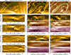 |
Fig. 1. Examples of atypical loop evolution events. Panel a presents the HRIEUV image, with two sets of yellow and green lines outlining the locations of the artificial slits that were used to derive the space-time (x-t) maps shown in panels a.1–a.4. The white, blue, and green arrows in these x-t maps mark the times when split-drift-type events are observed. The three loop structures where these events occur are marked with arrows in panel a. Panels b and c present the co-temporal images recorded in the AIA 171 Å and 193 Å passbands, while the x-t maps derived using these data are shown in panels b.1–c.6. The white, blue, and green arrows on these x-t maps mark the identical timestamps of their HRIEUV counterparts. In b.4–b.6, the green arrow indicates the only event captured by S |


While the loops appear visually similar in the HRIEUV and AIA 171 Å images, subtle differences emerge due to the LOS integration effects, owing to the 43° separation angle between the two spacecraft during this observation. This discrepancy is especially noticeable near the footpoints, where the loop curvature enhances the effect. Nevertheless, the superior resolution of HRIEUV allows for a clearer view of the loops and their evolution compared to AIA. However, the HRIEUV data are available in only one passband (174 Å, sampling plasma at 1 MK), whereas AIA spans a broader temperature range (0.6–10 MK) with six EUV passbands. Most of the loops we are interested in are not visible in the majority of AIA passbands, so we focused our analysis on the 171 Å, 193 Å, and 211 Å channels, where the loops can be reliably identified.
3.2. The multiwavelength aspect
We first examined the multiwavelength signatures of these events as well as signatures of such evolution at different positions along the length of these loops.
Slits S and S
and S cover the lowermost loop (loop-1 in Fig. 1a), and the two HRIEUV space-time (x-t) maps derived from these two different slits are shown in Figs. 1a.1 and 1a.2. These two specific slit locations were selected to investigate the extent of the effect of a split-drift event along the length of a loop while ensuring that the signal remains adequate at both slit locations. These x-t maps show similar trends of evolution, although the motions are less prominent in the S
 slit. This is expected, as this particular slit is located slightly farther from the loop top (adjudged visually). The same loop system is also visible in the AIA images, and the evolution captured in the two 171 Å x-t maps2 (Figs. 1b.1 and 1c.1) appears similar to that captured in the HRIEUV maps. However, they appear completely different in the 193 Å (Figs. 1b.2 and 1c.2) and 211 Å x-t maps (Figs. 1b.3 and 1c.3). For example, the S
 map shows no noticeable shift of the loop but rather a thick, bright structure staying put at the same location over the remaining time. The S
 map also captures a similar pattern. On the other hand, we see clear signatures of movement in the S
 and S
and S maps that cover the same loop at a different location. This makes the multiwavelength evolution difficult to explain. Additionally, the 171 Å maps reveal that around t = 40 min, the separated loop (or the thread) retracts back to its original position, where the initial movement began. However, no such trend exists in the 193 Å and 211 Å maps. Lastly, the initial split in the S
 map (highlighted by the white arrow) appears approximately a minute later than that in the S
 map.
map.
The loops next to loop-1 also show similar split-drift evolution. In fact, multiple instances of this type are captured in the S map (Fig. 1a.3). The overall evolution appears similar to that in the previous case. As we move toward the loop top, however, the splitting signatures become difficult to isolate from the background structures revealed in the S
 map (Fig. 1a.4). It is also noteworthy that the two instances, highlighted by the blue arrows in Fig. 1a.3, occur simultaneously with the split event seen in loop-1 (highlighted by the white arrow in Fig. 1a.1). The AIA data, however, could resolve only one (highlighted with the green arrow) out of the three cases. The S
 map captured a clear split-drift of the loop starting at t = 39 min. Unlike loop-1, the evolution captured in the 193 Å and 211 Å passbands3 is similar to that captured in the 171 Å map. On the other hand, the S4 x-t maps show signatures similar to those in the S1 maps from loop-1. Namely, the S
 map shows the loop moving, while the co-temporal S
 and S
and S maps show no movements.
3.3. The magnetic field underneath
Often, the dynamics at the coronal heights are a response to changes in the magnetic field at the photospheric height. In this section we investigate this relationship. The Polarimetric and Helioseismic Imager (PHI, Solanki et al. 2020), the magnetometer on board the Solar Orbiter, captured only a portion of the EUI field of view (FOV), which unfortunately lay outside the loops we are interested in. Therefore, we utilized the LOS magnetogram from the HMI for our analysis. The loop system is located on a relatively weak magnetic patch, away from the active region (see Fig. A.1). The footpoints on the east side are anchored in a positive polarity patch (indicated by the red contours), while the footpoints on the west side are situated in a negative polarity patch (shown by the cyan contours).
The animation associated with Fig. 2 reveals that in the coronal images, the west-side footpoint of the loop exhibits significant movement during the split-drift motion of the loop. To investigate this in detail, we selected six time instances (t1–t6, as marked in Fig. 2) that cover the entire sequence of the event, including the periods before, during, and after the loop split. Close-ups of this footpoint region, with magnetic field contours overlaid, are shown in the side panels of Fig. 2. We observe that this loop footpoint seems to jump back and forth between two negative polarity patches during the split event. For instance, at time t1 (before the split), the footpoint is rooted in the larger negative polarity patch near the top of the inset image. By time t3 (after the split), it has moved to the lower patch. Subsequently, at time t5 (and at t6), when the loop has retracted to its initial location, the footpoint also returns to the upper patch. These two polarity patches are separated by a distance of 5 Mm. In comparison, the loop top only moved about 3 Mm, according to the Fig. 1c.1 x-t map. At the same time, we observe that the magnetic patches themselves do not move around appreciably over the course of the loop evolution.
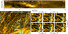 |
Fig. 2. Associations with the photospheric magnetic field. Panel a presents the x-t map from S |

Linking loop footpoints identified in EUV images to the photospheric magnetic patches recorded in magnetograms is not always straightforward (Chitta et al. 2017; Judge et al. 2024). Factors such as low-lying foreground or background structures in the EUV images, loop geometry and magnetic field expansion, and the resolution of the magnetic field data can play a significant role in this process. Consequently, the footpoints of the loops may be rooted (in the photospheric layer) in locations different from where they appear in the coronal images. Nonetheless, in all the cases shown in Fig. 1, we observe oscillatory motions accompanying such split-drift events. In the following section, we discuss these oscillations.
3.4. Presence of kink oscillations
Figure 3 provides zoomed-in views of three x-t maps taken from Fig. 1. We observe signatures of transverse oscillations occurring not only after but also before the loop’s split and, in some cases, in both situations. This raises questions about whether these oscillations cause the observed splits or simply respond to the sudden separation events. Nonetheless, most of these oscillations appear to survive multiple cycles without a noticeable decrease in their amplitudes4. The derived amplitudes and period values, as shown in Fig. 3, are typical of decayless kink oscillations reported in the literature (Anfinogentov et al. 2015; Mandal et al. 2022). This adds further complexity to our findings. For example, in loop-1, the low amplitude observed does not align with the expected wave amplitude, if the wave is a result of footpoint movement, as discussed in the previous section (one would anticipate a significantly larger amplitude in that case given the exponential drop in density).
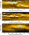 |
Fig. 3. Zoomed-in views of the kink oscillations occurring in the loops. Panels a.1, a.2, and a.3 display portions of the x-t maps derived from slits S |


3.5. Cross-field drift speeds
As mentioned earlier, we observe two distinct types of cross-field movements during these events: (i) movement of a thread-like structure that separates from the main loop; and (ii) movement of the separated thread toward its new location and later to its initial position. The animations associated with Fig. 1 demonstrate that these two speeds are notably different. We quantitatively established this by measuring the slopes of the bright ridges of the x-t maps as presented in Fig. 4. The sudden thread separation occurs with speeds of ≈30 km s−1 (slopes drawn with cyan lines), while the loops drift much more slowly, with speeds of ≈5 km s−1 (slopes drawn with white lines). These speeds do not correspond to any characteristic velocities typically observed in the lower corona. However, since these speeds consistently appear across all events, it is reasonable to think they are associated with the driver that triggers these split-drift cases. One possibility is that these speeds reflect the motion of the loop footpoints, which move with the granular flow, typically at a rate of 1–2 km s−1. However, in most cases, the drift speeds are 2–3 times higher than these values. As presented in Sect. 3.3, the magnetic patches at the photosphere do not seem to move significantly, and therefore, these speeds likely do not have a direct connection to the photosphere. Still, considering the strong density gradient between the photosphere and the corona, it is possible that the relatively slow drift speeds in the photosphere could lead to much faster changes in the upper atmosphere. However, this effect may be limited to scenarios involving faster footpoint driving (leading to waves) and may not apply to the slower driving associated with quasi-static evolution.
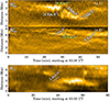 |
Fig. 4. Estimation of the drift speeds of the loops. The x-t maps are the same as those in Fig. 3. To guide the eye, the white slanted lines outline the slopes that indicate the drift speeds of the loops, while the two green lines represent the slopes associated with the loop splits. The derived speed values are printed on the panels. |
Additionally, chromospheric and transition region features, such as dynamic fibrils or spicules, exhibit characteristic speeds of 15–30 km s−1 (Mandal et al. 2023). These are similar to the drift speeds observed in this work. Even so, it remains unclear how the field-aligned speeds of spicules or dynamic fibrils relate to the transverse (to the field) drift speeds of the observed loops. Furthermore, spicules exhibit transversal motions with wave amplitudes of about 20 km s−1 (de Pontieu et al. 2007). It remains unclear how such chromospheric oscillations could lead to the split-drift motions observed closer to the coronal apexes of loops (e.g., slits 1, 2, and 4 in Fig. 1). The small-scale interchange reconnection at the footpoints of these loops is a potential source. The loops we studied are anchored in weak plage or network structures located away from the core of the active region. Here, magnetoconvection coupled with dynamic parasitic polarity activity on short timescales of less than 5 minutes could create disturbances in the corona (Chitta et al. 2023). While HMI magnetograms do indicate some evidence of scattered parasitic polarities near the footpoints of the coronal loops (Fig. 2), we cannot establish a clear one-to-one correspondence between potential small-scale interchange reconnection and the observed coronal loop drifts.
4. Summary and discussion
Let us first summarize the key features of these split-drift events. (i) Two characteristic speeds are involved: a faster (30 km s−1) outward movement of a thin, thread-like structure and a substantially slower (5 km s−1) drift speed of the parent or detached loop. (ii) Kink oscillations are present before or after the split, and sometimes at both instances. (iii) The back-and-forth movement of one of the loop footpoints is evident in the EUV coronal images. The LOS magnetogram data confirm the presence of two similar polarity patches where the footpoints shift. However, the magnetic patches (in the HMI data) themselves do not move in the process. (iv) The evolution of these events in cooler channels (such as in AIA 171 Å or in HRIEUV) does not always correspond to what is observed in hotter channels (such as in AIA 193 Å or in the 211 Å passbands).
Several aspects of the observed loop evolution remain challenging to interpret. For instance, in loop-1, the evolution captured in different AIA channels appears completely different with respect to the loop’s position. This observation is inconsistent with the typical multi-thermal loop model (Schmelz et al. 2009), which suggests similarities in the evolution patterns between the AIA 171 and the AIA 193 maps, as the response functions of these two passbands overlap. One possible explanation could be the presence of multiple (at least three) overlapping strands with specific temperature profiles that cause them to selectively appear or disappear in a particular AIA passband. The AIA 193 Å image in Fig. 1c indeed shows two overlapping strands at the slit-1 location, potentially explaining the apparent stationary appearance of one strand in that slit. However, requiring such specific temperature profiles seems somewhat contrived, and thus this scenario seems unlikely. On the other hand, a closer look at the AIA data hints at the multi-thermal nature of these strands. The intensity of a prominent bright loop, which remains stationary in the AIA 193 Å map (Fig. 1b.2), significantly decreases right after the split is observed in the AIA 171 Å map, further suggesting multi-thermality. The long-term loop intensity evolution discussed in Paper I provides additional evidence for this. Still, the rapid change in a strand’s appearance across two AIA passbands within a few minutes remains puzzling. In Fig. 1a.2 we find enhanced emission prior to the split. This could be interpreted as a signature of localized heating (or cooling). However, as outlined in Sect. 3.2, the evolution in the hotter channels appears quite different and does not conform to a single scenario. Furthermore, such intensity enhancements are not immediately apparent in other events. Therefore, at this point, we do not have conclusive evidence of localized heating or cooling events.
Another intriguing aspect is the lack of kink oscillation signals in the AIA 193 Å and AIA 211 Å maps, despite their presence in the AIA 171 Å map. As mentioned earlier, the oscillation parameters observed are characteristic of decayless kink oscillations reported in the literature. However, unlike typical kink oscillations, which usually appear across multiple AIA passbands (Wang et al. 2012; Mandal et al. 2021), the oscillations in this study do not. This discrepancy may support the idea of a multistrand loop structure with unusual temperature profiles. The absence of oscillation signals in the hotter passbands could also be attributed to the diffuse nature of the hotter plasma (Tripathi et al. 2009), which may obscure oscillation signatures. However, this trend is not universal across maps. For example, the loops in S and S
and S appear relatively compact. Once again, a coherent picture does not emerge from all the events analyzed.
The pattern of speeds with which the loop drifts seems to be consistent across events (Fig. 4). As discussed in Sect. 3.3, the magnetic patches in the photosphere near one of the loop footpoints remain stationary, while the EUV footpoint exhibits significant back-and-forth movement. This observation suggests that the origin of this movement likely occurs in the layers above the photosphere. As shown in Fig. A.2e, the cooler 304 Å passband data do not indicate the presence of low-lying filament-like structures. Therefore, the height and nature of the perturbation that drives these split-drift events remain unclear at this point. Additionally, as mentioned in Sect. 3.3, we should exercise caution when associating the footpoints derived from EUV images with their counterparts in the lower atmosphere.
Considering the points we have discussed thus far, it appears that magnetic reconnection could be a plausible source driving these split-drift events. The rapid timescale of these splits (occurring in under a minute) and the oscillations observed after the split agree well with the idea that these events result from magnetic reconnection. Conceptually, it is straightforward to imagine two slightly misaligned magnetic field lines reconnecting through the “component reconnection” mechanism, forming structures that drift away perpendicularly (Pagano et al. 2021). Moreover, invoking such reconnections at different locations along a strand – caused by interactions with multiple other strands – can easily explain the return of the loops. According to this picture, the observed loop motions relate to the actual motion of the field lines. However, this scenario is not without caveats. For example, none of the cases analyzed here exhibited the typical outflowing jet-like features (“nanojets”) commonly associated with such reconnection events (Antolin et al. 2021), nor do they show sudden brightenings associated with an untangling of braided loops (Chitta et al. 2022). Furthermore, the heating associated with reconnection is generally impulsive in nature, and it takes considerable time (approximately 1000 seconds) for the emission to become visible in most observing channels (Klimchuk et al. 2008).
Nevertheless, this does not rule out the reconnection hypothesis. Reconnected field lines demonstrate real motion near the reconnection site, where the outflows can be extremely fast. However, as we move away from the site, this motion becomes limited and disappears entirely at the line-tied footpoints, with the exception of unrelated, slower photospheric flows at approximately 1 km s−1. In contrast to these real motions, there are apparent motions caused by the successive heating and cooling of adjacent field lines. Reconnected field lines become bright when the hot evaporated plasma resulting from impulsive heating cools through the range of temperature sensitivity of the observing channel. The rate at which this effect propagates perpendicular to the field – which is the speed of the apparent motion – is determined by the rate at which magnetic flux is processed by the reconnection. Typically, reconnection inflow velocities are around 1% of the local Alfvén speed5 based on the reconnecting (shear) field component, or roughly 10–30 km s−1. Thus, the apparent drift of a bright strand should be comparable to this speed well away from the reconnection site. This is consistent with what we observe. We note that an apparent drift associated with cooling would initially appear in the 211 Å and 193 Å channels, and subsequently in the 171 Å channel. This is consistent with the observations. In this picture, however, it is challenging to understand how the thread returns to its initial position, as seen in some of our events.
Another type of apparent motion related to successive heating and cooling is associated with phenomena known as “magnetic flipping” (Priest et al. 2003; Pontin et al. 2005) and “slip-running” reconnection Aulanier et al. (2006). The speeds in these cases can be very fast – potentially even super-Alfvénic – depending on the thickness of the reconnecting current sheet. These apparent motions occur parallel to the current sheet, while the motions discussed earlier are perpendicular. The discussion above raises a couple of key questions: (i) Given that such observations are rare in coronal loops (with the events discussed in Aulanier et al. 2007 sharing some similarities with those addressed here), what conditions must be met for these occurrences to be observed more frequently? (ii) Which factors, including projection effects, determine whether the apparent speeds are sub- or super-Alfvénic? Unfortunately, the data we have for these events are insufficient to answer these questions. Therefore, in the future, we need to conduct a statistical study of loops at different positions on the solar disk. Additionally, examining a realistic multistrand loop model, such as the one presented in Breu et al. (2022), may help clarify the role of reconnection in producing the observed dynamics in these loops.
5. Conclusion
We have presented several examples of unusual, cross-field motions of coronal loops. These events are characterized by the presence of kink oscillations both before and after the occurrences, along with distinct fast (30 km s−1) and slow (5 km s−1) cross-field drift speeds. Additionally, there is a noticeable back-and-forth movement of the loop footpoints between magnetic polarity patches. While we have discussed several possible drivers (e.g., magnetic reconnection), a comprehensive understanding of these events is still lacking. To gain deeper insight into this phenomenon, future studies with larger statistical samples are necessary.
Data availability
Movies associated to Figs. 1 and 2 are available at https://www.aanda.org
Publicly available via the Solar Orbiter/EUI Data Release 6.0 (Kraaikamp et al. 2023).
Note that the position of the AIA slits appears different from those of the HRIEUV due to the distinctly different vantage points of the two spacecraft.
The signal in 211 Å is significantly weak, and the loop can only be identified in hindsight, i.e., only after looking at the 171 Å and 193 Å x-t maps.
Even though the oscillation in Fig. 3(a.1) starting at 30 min is not as clear as the earlier oscillation in the same panel, the sinusoidal fit is still much better than, e.g., a linear fit.
Although we do not have direct measurements of the magnetic field and the density of the loop, it is reasonable to assume typical coronal values for these parameters. This assumption would suggest a local Alfvén speed between 1000 and 3000 km s−1.
Acknowledgments
We thank the anonymous reviewer for their insightful comments. The EUI instrument was built by CSL, IAS, MPS, MSSL/UCL, PMOD/WRC, ROB, LCF/IO with funding from the Belgian Federal Science Policy Office (BELSPO/PRODEX PEA 4000112292 and 4000134088); the Centre National d’Etudes Spatiales (CNES); the UK Space Agency (UKSA); the Bundesministerium für Wirtschaft und Energie (BMWi) through the Deutsches Zentrum für Luft- und Raumfahrt (DLR); and the Swiss Space Office (SSO). We are grateful to the ESA SOC and MOC teams for their support. Solar Dynamics Observatory (SDO) is the first mission to be launched for NASA’s Living With a Star (LWS) Program. The data from the SDO/AIA consortium are provided by the Joint Science Operations Center (JSOC) Science Data Processing at Stanford University. The work of S.M. is funded by the Federal Ministry for Economic Affairs and Climate Action (BMWK) through the German Space Agency at DLR based on a decision of the German Bundestag (Funding code: 50OU2201). L.P.C. gratefully acknowledges funding by the European Union (ERC, ORIGIN, 101039844). Views and opinions expressed are however those of the author(s) only and do not necessarily reflect those of the European Union or the European Research Council. Neither the European Union nor the granting authority can be held responsible for them. The work of JAK was supported by the GSFC Heliophysics Internal Scientist Funding Model competitive work package program.
References
- Anfinogentov, S. A., Nakariakov, V. M., & Nisticò, G. 2015, A&A, 583, A136 [NASA ADS] [CrossRef] [EDP Sciences] [Google Scholar]
- Antolin, P., Pagano, P., Testa, P., Petralia, A., & Reale, F. 2021, Nat. Astron., 5, 54 [NASA ADS] [CrossRef] [Google Scholar]
- Aschwanden, M. J., Nitta, N. V., Wuelser, J.-P., & Lemen, J. R. 2008a, ApJ, 680, 1477 [NASA ADS] [CrossRef] [Google Scholar]
- Aschwanden, M. J., Wülser, J.-P., Nitta, N. V., & Lemen, J. R. 2008b, ApJ, 679, 827 [NASA ADS] [CrossRef] [Google Scholar]
- Aulanier, G., Pariat, E., Démoulin, P., & Devore, C. R. 2006, Sol. Phys., 238, 347 [NASA ADS] [CrossRef] [Google Scholar]
- Aulanier, G., Golub, L., DeLuca, E. E., et al. 2007, Science, 318, 1588 [CrossRef] [Google Scholar]
- Breu, C., Peter, H., Cameron, R., et al. 2022, A&A, 658, A45 [NASA ADS] [CrossRef] [EDP Sciences] [Google Scholar]
- Chitta, L. P., Peter, H., Solanki, S. K., et al. 2017, ApJS, 229, 4 [Google Scholar]
- Chitta, L. P., Peter, H., Parenti, S., et al. 2022, A&A, 667, A166 [NASA ADS] [CrossRef] [EDP Sciences] [Google Scholar]
- Chitta, L. P., Solanki, S. K., del Toro Iniesta, J. C., et al. 2023, ApJ, 956, L1 [NASA ADS] [CrossRef] [Google Scholar]
- de Pontieu, B., McIntosh, S., Hansteen, V. H., et al. 2007, PASJ, 59, S655 [NASA ADS] [CrossRef] [Google Scholar]
- Feng, L., Inhester, B., Solanki, S. K., et al. 2007, ApJ, 671, L205 [NASA ADS] [CrossRef] [Google Scholar]
- Judge, P. G., Kleint, L., & Kuckein, C. 2024, ApJ, 970, 147 [Google Scholar]
- Kaiser, M. L., Kucera, T. A., Davila, J. M., et al. 2008, Space Sci. Rev., 136, 5 [Google Scholar]
- Klimchuk, J. A. 2000, Sol. Phys., 193, 53 [NASA ADS] [CrossRef] [Google Scholar]
- Klimchuk, J. A. 2006, Sol. Phys., 234, 41 [Google Scholar]
- Klimchuk, J. A., & DeForest, C. E. 2020, ApJ, 900, 167 [NASA ADS] [CrossRef] [Google Scholar]
- Klimchuk, J. A., Lemen, J. R., Feldman, U., Tsuneta, S., & Uchida, Y. 1992, PASJ, 44, L181 [NASA ADS] [CrossRef] [Google Scholar]
- Klimchuk, J. A., Patsourakos, S., & Cargill, P. J. 2008, ApJ, 682, 1351 [Google Scholar]
- Kraaikamp, E., Gissot, S., Stegen, K., et al. 2023, SolO/EUI Data Release 6.0 2023-01, https://doi.org/10.24414/z818-4163, published by Royal Observatory of Belgium (ROB) [Google Scholar]
- Lemen, J. R., Title, A. M., Akin, D. J., et al. 2012, Sol. Phys., 275, 17 [Google Scholar]
- Mandal, S., Tian, H., & Peter, H. 2021, A&A, 652, L3 [NASA ADS] [CrossRef] [EDP Sciences] [Google Scholar]
- Mandal, S., Chitta, L. P., Antolin, P., et al. 2022, A&A, 666, L2 [NASA ADS] [CrossRef] [EDP Sciences] [Google Scholar]
- Mandal, S., Peter, H., Chitta, L. P., et al. 2023, A&A, 670, L3 [NASA ADS] [CrossRef] [EDP Sciences] [Google Scholar]
- Mandal, S., Peter, H., Klimchuk, J. A., et al. 2024, A&A, 682, L9 [NASA ADS] [CrossRef] [EDP Sciences] [Google Scholar]
- McCarthy, M. I., Longcope, D. W., & Malanushenko, A. 2021, ApJ, 913, 56 [NASA ADS] [CrossRef] [Google Scholar]
- Müller, D., St. Cyr, O. C., Zouganelis, I., et al. 2020, A&A, 642, A1 [Google Scholar]
- Pagano, P., Antolin, P., & Petralia, A. 2021, A&A, 656, A141 [NASA ADS] [CrossRef] [EDP Sciences] [Google Scholar]
- Pesnell, W. D., Thompson, B. J., & Chamberlin, P. C. 2012, Sol. Phys., 275, 3 [Google Scholar]
- Peter, H., & Bingert, S. 2012, A&A, 548, A1 [NASA ADS] [CrossRef] [EDP Sciences] [Google Scholar]
- Peter, H., Bingert, S., Klimchuk, J. A., et al. 2013, A&A, 556, A104 [NASA ADS] [CrossRef] [EDP Sciences] [Google Scholar]
- Pontin, D. I., Galsgaard, K., Hornig, G., & Priest, E. R. 2005, Phys. Plasmas, 12, 052307 [Google Scholar]
- Priest, E. R., Hornig, G., & Pontin, D. I. 2003, J. Geophys. Res. Space Phys., 108, 1285 [NASA ADS] [CrossRef] [Google Scholar]
- Reale, F. 2014, Liv. Rev. Sol. Phys., 11, 4 [Google Scholar]
- Rochus, P., Auchère, F., Berghmans, D., et al. 2020, A&A, 642, A8 [NASA ADS] [CrossRef] [EDP Sciences] [Google Scholar]
- Scherrer, P. H., Schou, J., Bush, R. I., et al. 2012, Sol. Phys., 275, 207 [Google Scholar]
- Schmelz, J. T., Nasraoui, K., Rightmire, L. A., et al. 2009, ApJ, 691, 503 [Google Scholar]
- Solanki, S. K., del Toro Iniesta, J. C., Woch, J., et al. 2020, A&A, 642, A11 [NASA ADS] [CrossRef] [EDP Sciences] [Google Scholar]
- Tripathi, D., Mason, H. E., Dwivedi, B. N., del Zanna, G., & Young, P. R. 2009, ApJ, 694, 1256 [CrossRef] [Google Scholar]
- Wang, T., Ofman, L., Davila, J. M., & Su, Y. 2012, ApJ, 751, L27 [Google Scholar]
Appendix A: Overall magnetic configuration
In Fig. A.1 we provide an overview of the magnetic structure adjacent to the loop system studied in this work. As shown in panel b, the loop system is located away from an active region, where the magnetic field is relatively weaker near both of its footpoints. The footpoints on the west side are anchored within negative polarity patches, while the footpoints on the east side (not fully visible) are anchored in positive polarity patches.
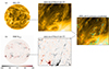 |
Fig. A.1. Images of the solar disc as recorded through the AIA 171 Å passband and the HMI-LOS are shown in panel a and panel b, respectively. The black rectangle in each panel outlines the region of interest (ROI) that encompasses the loop system studied in this paper. Panels a.1 and b.1 provide additional images of the ROI for the AIA and HMI data, respectively. In panel c, the cyan and red contours, representing the boundaries of ±40 G as derived from panel b.1, are overlaid on the AIA image from panel a.1. |
We also include Fig. A.2 that presents images from different AIA passbands. This figure provides an overview of the multi-thermal structuring of the entire region. For example, in the 94 Å snapshot, we observe very faint emissions from the overarching loops, which are likely much hotter. In contrast, these emissions are entirely absent from the cooler chromospheric (and transition region) emission captured in the 304 Å emissions.
All Tables
All Figures
|
Fig. 1. Examples of atypical loop evolution events. Panel a presents the HRIEUV image, with two sets of yellow and green lines outlining the locations of the artificial slits that were used to derive the space-time (x-t) maps shown in panels a.1–a.4. The white, blue, and green arrows in these x-t maps mark the times when split-drift-type events are observed. The three loop structures where these events occur are marked with arrows in panel a. Panels b and c present the co-temporal images recorded in the AIA 171 Å and 193 Å passbands, while the x-t maps derived using these data are shown in panels b.1–c.6. The white, blue, and green arrows on these x-t maps mark the identical timestamps of their HRIEUV counterparts. In b.4–b.6, the green arrow indicates the only event captured by S |
| In the text | |
|
Fig. 2. Associations with the photospheric magnetic field. Panel a presents the x-t map from S |
| In the text | |
|
Fig. 3. Zoomed-in views of the kink oscillations occurring in the loops. Panels a.1, a.2, and a.3 display portions of the x-t maps derived from slits S |
| In the text | |
|
Fig. 4. Estimation of the drift speeds of the loops. The x-t maps are the same as those in Fig. 3. To guide the eye, the white slanted lines outline the slopes that indicate the drift speeds of the loops, while the two green lines represent the slopes associated with the loop splits. The derived speed values are printed on the panels. |
| In the text | |
|
Fig. A.1. Images of the solar disc as recorded through the AIA 171 Å passband and the HMI-LOS are shown in panel a and panel b, respectively. The black rectangle in each panel outlines the region of interest (ROI) that encompasses the loop system studied in this paper. Panels a.1 and b.1 provide additional images of the ROI for the AIA and HMI data, respectively. In panel c, the cyan and red contours, representing the boundaries of ±40 G as derived from panel b.1, are overlaid on the AIA image from panel a.1. |
| In the text | |
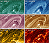 |
Fig. A.2. Snapshots from different AIA passbands of the same FOV shown in Fig. 1. |
| In the text | |
Current usage metrics show cumulative count of Article Views (full-text article views including HTML views, PDF and ePub downloads, according to the available data) and Abstracts Views on Vision4Press platform.
Data correspond to usage on the plateform after 2015. The current usage metrics is available 48-96 hours after online publication and is updated daily on week days.
Initial download of the metrics may take a while.