| Issue |
A&A
Volume 682, February 2024
Solar Orbiter First Results (Nominal Mission Phase)
|
|
|---|---|---|
| Article Number | L9 | |
| Number of page(s) | 11 | |
| Section | Letters to the Editor | |
| DOI | https://doi.org/10.1051/0004-6361/202348776 | |
| Published online | 09 February 2024 | |
Letter to the Editor
Investigating coronal loop morphology and dynamics from two vantage points⋆
1
Max Planck Institute for Solar System Research, Justus-von-Liebig-Weg 3, 37077 Göttingen, Germany
e-mail: This email address is being protected from spambots. You need JavaScript enabled to view it.
2
NASA Goddard Space Flight Center, Greenbelt, MD, USA
3
School of Space Research, Kyung Hee University, Yongin, Gyeonggi 446-701, Republic of Korea
4
Solar-Terrestrial Centre of Excellence – SIDC, Royal Observatory of Belgium, Ringlaan -3- Av. Circulaire, 1180 Brussels, Belgium
5
Université Paris-Saclay, CNRS, Institut d’Astrophysique Spatiale, 91405 Orsay, France
Received:
28
November
2023
Accepted:
13
January
2024
Abstract
Coronal loops are the fundamental building blocks of the solar corona. Therefore, comprehending their properties is essential in unraveling the dynamics of the upper solar atmosphere. In this study, we conduct a comparative analysis of the morphology and dynamics of a coronal loop observed from two different spacecraft: the High Resolution Imager (HRIEUV) of the Extreme Ultraviolet Imager on board the Solar Orbiter, and the Atmospheric Imaging Assembly (AIA) on board the Solar Dynamics Observatory. These spacecraft were separated by 43° during this observation. The main findings of this study are that (1) the observed loop exhibits similar widths in both the HRIEUV and AIA data, suggesting that the cross-sectional shape of the loop is circular; (2) the loop maintains a uniform width along its entire length, supporting the notion that coronal loops do not exhibit expansion; and (3) notably, the loop undergoes unconventional dynamics, including thread separation and abrupt downward movement. Intriguingly, these dynamic features also appear similar in data from both spacecraft. Although based on observation of a single loop, these results raise questions about the validity of the coronal-veil hypothesis and underscore the intricate and diverse nature of the complexity within coronal loops.
Key words: Sun: atmosphere / Sun: corona / Sun: magnetic fields / Sun: oscillations / Sun: UV radiation
Movie associated to Fig. 1 is available at https://www.aanda.org.
© The Authors 2024
 Open Access article, published by EDP Sciences, under the terms of the Creative Commons Attribution License (https://creativecommons.org/licenses/by/4.0), which permits unrestricted use, distribution, and reproduction in any medium, provided the original work is properly cited.
This article is published in open access under the Subscribe to Open model.
Open access funding provided by Max Planck Society.
1. Introduction
Coronal loops, characterized by their bright, curved, tube-like appearance, are some of the most easily recognizable features within the solar corona. Traditionally, these loops have been understood in terms of plasma confinement within arched magnetic field lines that extend into the low-β corona. Depending on the wavelength at which they are observed, the plasma inside a loop is hotter and/or denser than the surroundings. This causes them to appear bright. Over the years, regular observations of the corona in the extreme-ultraviolet (EUV) and X-ray wavelengths, where these loops are most prominently visible, have led to a plethora of research to understand their properties and evolution (Reale 2014), including a stereoscopic determination of the loop geometry, density, and temperature (Feng et al. 2007; Aschwanden et al. 2008a,b).
Among others, the shape of a coronal loop remains a topic of interest among researchers. Observations typically reveal that these loops maintain a consistent width or cross-sectional diameter along their entire length (Klimchuk et al. 1992; Klimchuk 2000; López Fuentes et al. 2006). This is in stark contrast to our current magnetic extrapolation models that predict an expansion of the magnetic field with height above the solar surface. Several potential explanations have been proposed for this apparent discrepancy, including the presence of twist in the field lines (Klimchuk et al. 2000), a magnetic separator that expands less strongly (Plowman et al. 2009), a combination of the thermal structuring of the loop and the spectral properties of the imaging instrumentation (Peter & Bingert 2012), and a preferential expansion in the line-of-sight direction (Malanushenko & Schrijver 2013). However, none of these proposed solutions have been universally proven to apply to all types of loops and in different magnetic environments, such as active regions and the quiet Sun.
Another related issue is the cross-sectional structure of coronal loops. In EUV images, the cross section of a loop often appears to be symmetric and is typically modeled using a Gaussian profile. This prompted researchers to conclude that a coronal loop possesses a circular cross section (e.g., Klimchuk 2000). However, it is unclear why the heating would be symmetrical (a symmetrically spreading avalanche of nanoflares is one possibility; Klimchuk et al. 2023), and therefore, why a loop would have a circular cross section. Nonetheless, it is important to note that like many other studies of the solar corona, assessments of loop properties are also affected by the optically thin nature of the coronal emission. Features in the background or foreground contaminate the measurements (McCarthy et al. 2021), although results about a constant loop width may still hold true (López Fuentes et al. 2008).
An alternative interpretation of the cross-sectional loop profile is the so-called coronal-veil hypothesis (Malanushenko et al. 2022). According to this hypothesis, loops are a line-of-sight effect of warped sheets of bright emission. This scenario is similar to how wrinkles appear in a veil. However, similar to other aspects of this model picture, to evaluate the cross-sectional shape of loops, it is imperative to observe the same loop from different vantage points, which results in two distinct line-of-sight integrations.
In this study, we compare the dynamics and morphology of a coronal loop viewed from two spacecraft that at the time of the observations analyzed here, subtended a 43° angle at the Sun. We used co-temporal high-resolution EUV images of the corona taken from the Solar Dynamics Observatory (SDO; Pesnell et al. 2012) and the Solar Orbiter spacecraft (Müller et al. 2020). This approach enabled us to further investigate the properties of the loop in connection with the coronal-veil hypothesis.
2. Data
We used EUV images taken on April 7, 2023 by Solar Orbiter and SDO. We used EUV images from the High Resolution Imager (HRIEUV; taken via the 174 Å bandpass) of the Extreme Ultraviolet Imager (EUI; Rochus et al. 2020), which samples plasma with a temperature of about T ≈ 1 MK. This HRIEUV dataset1 has a cadence of 10 s, it lasted for one hour, and its image scale is 0.492″ pix−1. On this day, Solar Orbiter was at a distance of about 0.3 astronomical units (au) from the Sun, meaning that the HRIEUV images have a plate scale of 108 km pix−1 on the Sun. Solar Orbiter was about 43° away from the Sun-Earth line. Additionally, we combined the HRIEUV data with full-disk EUV images from the Atmospheric Imaging Assembly (AIA; Lemen et al. 2012) on board the Earth-orbiting SDO. Specifically, we analyzed data from the 171 Å (sensitive to plasma of 0.8 MK), 193 Å (1.6 MK), and 211 Å (2.0 MK) AIA passbands, each with a cadence of 12 s and a plate scale of 0.6″ pix−1 (corresponding to 435 km pix−1 on the Sun). While the spatial resolution of the HRIEUV data is almost four times better than the resolution of the AIA data, both datasets have similar temporal resolution. Last, while comparing the HRIEUV and AIA images, we took the difference in light propagation time from the Sun to Solar Orbiter into account, which was 0.3 au away from the Sun, and the propagation time to SDO, which was 1 au away from the Sun. All the time-stamps quoted here are the times as measured at Earth.
3. Results
We focused on a coronal loop situated on the northwest side of active region NOAA AR13270, which is at the center of the HRIEUV field of view (see Fig. A.1). It is important to note that Solar Orbiter was at an angle of 43° with SDO when the observation was made, as shown in Fig. 1a. By combining images from AIA and HRIEUV, we were able to obtain a stereoscopic view of the loop and its dynamics.
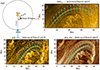 |
Fig. 1. Overview of the event. Panel a depicts the relative position of the two spacecraft, SDO and Solar Orbiter, whose data are used in this study. Panel b shows the loop under study in the HRIEUV image, and panels c and d show the same loop, but as seen in the AIA 171 Å and 193 Å channels, respectively. The cyan lines highlight the locations of the artificial slits that are used to generate space-time maps (shown in Figs. 2, 3, 7 and B.1). The arrow in the center of each slit indicates the direction of increasing distance along the slit. The images in panels b–d are unsharp-masked for an improved visibility of the loop. A movie is available online. |
3.1. Comparing the loop dynamics
In the animation shown in Fig. 1, we find a loop (or a group of threads) that first appears about 03:45 UT. It gradually becomes brighter over time and undergoes various dynamic changes. This evolution appears similar in the HRIEUV and AIA data, even though the latter instrument was at an angular distance of 43° from the former. To quantitatively analyze the loop evolution, we placed multiple artificial slits along its length, as shown in Figs. 1b–d. Through these slits, we aimed to capture the loop dynamics, including any oscillations that occurred perpendicular to the loop. It is important to clarify that because our goal is to study the overall characteristics of the loop, we did not align these artificial slits precisely in exactly the same positions in the two images. We instead aimed to place them nearby because establishing a pixel-level correspondence between these two datasets is challenging.
The space-time (x-t) maps for a set of artificial slits are presented in Fig. 2. We first focus on the HRIEUV x-t map (panel a). The loop (at x = 3 Mm) gradually brightens starting from t = 15 min. Then, starting at t = 27 min, it undergoes transverse oscillations, as indicated by the sinusoidal pattern in the map (also visible in the animation). While the oscillations were present, a thin thread-like structure appears to separate from the loop and to move away. Panel a.1 presents a closer view of this segment. The thread stops moving after traveling almost 1.6 Mm along the slit in just one minute. Interestingly, the entire loop bundle (from which the thin thread is detached) is also observed to be displaced (ending at around the x = 4.6 Mm mark) by almost the same distance of 1.6 Mm as the thin thread. The extent of this motion is highlighted by two vertical dashed lines in panel a. Again, this movement also occurs over a timescale of one minute. Eventually, the shifted loop gradually fades away. In summary, the HRIEUV images display a loop that moves rapidly in the transverse direction by ∼1.6 Mm within one minute.
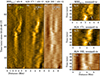 |
Fig. 2. Representative examples of space-time (x-t) maps derived from the HRIEUV (panel a), AIA 171 Å (panel b), and AIA 193 Å (panel c) image sequences. Zoomed-in versions of these maps, between t = 30 min and 40 min, are presented in panels a.1, b.1, and c.1, respectively. The arrows in these zoomed-in panel point to the slanted ridge that is created by the thin strand. The vertical dotted lines in these panels outline the shift of the loop as judged visually. |
In the next step, we analyzed the AIA images. Panels b and c of Fig. 2 show the x-t maps for the 171 Å and 193 Å channels, respectively2. The loop evolution in the 171 Å channel appears to be similar to the evolution in the HRIEUV, although the lower spatial resolution of AIA is noticeable in the map. Nevertheless, the thin thread can also be identified in this map (panel b.1), primarily due to our prior knowledge about it from HRIEUV data. Remarkably, we found the displacement of the loop (located at x = 3.5 Mm) in the 171 Å channel to be similar (1.8 Mm, as highlighted by two vertical dashed lines) to that of HRIEUV (1.6 Mm), even though the two instruments were 43° apart. This result suggests that the plane of motion of the loop (and the thin thread) is roughly perpendicular to the solar surface.
Interestingly, the 193 Å channel map (panel c of Fig. 2) shows not only similarities, but also significant differences when compared to the 171 Å and HRIEUV maps. For example, between t = 15 min and t = 22 min, the loop (located at x = 3.5 Mm) appears to be significantly brighter in the 193 Å map than in the 171 Å map. Furthermore, at x = 5.3 Mm (the second vertical line), a bright loop is visible in the 193 Å map, while no such structure appears in the 171 Å map. In contrast, between t = 22 min and 32 min, the loop is clearly discernible in the 171 Å map, but it appears to be somewhat blurry in the 193 Å map. Moreover, the comparison of the times after which the loop suddenly moves downward in the 171 Å data makes this even more intriguing. In the 193 Å map, a loop is visible exactly where it eventually settles in the 171 map after the movement (i.e., at x = 5.3). However, a loop is also continuously visible in the 193 Å map at the position3 of the loop before the movement (x = 3.5). Therefore, in this scenario, the loop moves downward in the 171 Å map, but the 193 Å map shows two loops, one loop at the shifted loop position, and the other loop in the position of the loop before the shift.
3.2. Comparing loop morphology
We analyzed the shape and appearance of the loop as seen through HRIEUV and AIA 171 Å images. These analyses were performed on the raw data, not on the edge-enhanced images.
At first glance, the shape and evolution appear to be quite similar in HRIEUV and AIA (Fig. 2). To quantitatively compare the two, we examined the width (via cross-sectional intensity) of the loop at three different times: before, during, and after the sudden movement of the loop, as highlighted in Fig. 3. The loop width appears to be similar in HRIEUV and 171 Å at all three instances. This also provides information about the shape of the loop cross section. This shape is still actively debated in the community (Klimchuk 2000; Klimchuk et al. 2000; Malanushenko & Schrijver 2013; Williams et al. 2021; Uritsky & Klimchuk 2024). If the loop has an elliptical cross section, changes in the measured cross-section values (and therefore, in cross-sectional intensities) are expected, when viewed from 43° apart. However, as revealed in Fig. 3, no such difference is observed. Therefore, we conclude that the loop cross section is nearly circular, consistent with previous studies, for instance, by Klimchuk (2000) and Klimchuk & DeForest (2020). In addition to this, Fig. 3d shows that the two structures, the parent loop and the thin thread, are clearly resolved in HRIEUV (the green curve). Interestingly, although the spatial resolution is four times coarser than that of HRIEUV, AIA (the red curve) also captured the small thread, if only just. Moreover, it is also evident that without the assistance from the HRIEUV image, the 171 Å feature would likely not be considered as a signature of the thread.
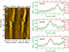 |
Fig. 3. Comparison of loop widths from HRIEUV and AIA. Panels a and b show x-t maps from HRIEUV and AIA, respectively. The intensity (DN s−1) along the respective colored dashed lines (marked with “t”) is plotted in panels c–e. Panel c shows the derived curves from HRIEUV (green curve) and AIA 171 Å (red) data at t = t3. The curves from t = t2 and t1 are shown in panels d and e, respectively. |
Next, we examined the loop width along the length of the loop. We show in Fig. 4 the loop intensities along different slits that are placed perpendicular to the loop length, as shown in Fig. 1. The time at which these loop intensities were derived is identical to the time shown in Fig. 1. For a better understanding of the overall behavior, we applied running averages on the curves. We used 8 pixels in HRIEUV and 2 pixels in AIA, taking the four-fold resolution difference between these two instruments into account. This smoothing process effectively mitigated minor fluctuations. Moreover, in order to avoid a low signal-to-noise ratio, we limited our analysis of the HRIEUV data to the region spanning from slit 1 to slit 10. Regardless, through these slits, we covered more than half of the total loop length. Our analysis yielded two crucial outcomes. (a) The loop width remains remarkably consistent along its length in images from both spacecrafts. This characteristic is more prominently captured in HRIEUV data because their spatial resolution is higher. Furthermore, the proximity of a moss-type structure adjacent to the AIA loop section near slits 4 to 7 affects the shape of the intensity curves from these slits, resulting in distortion and broadening. (b) The loop width as observed from the HRIEUV and AIA perspectives, is aligned along its length (the full width at half maximum (FWHM) is roughly 1.6 Mm in both datasets). Because the loop is not completely aligned with the plane spanned by the vantage points of the spacecraft4, these results suggest that the loop maintains a nearly circular cross section throughout its entire extent.
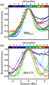 |
Fig. 4. Variation in the loop width along its length. Panel a shows the normalized HRIEUV intensities calculated along different slits (highlighted via the color bar). The same but for the AIA 171 Å data is shown in panel b. The time at which these loop intensities were derived is identical to the time shown in Fig. 1. Each curve is adjusted to ensure that its peak lies at x = 0 Mm. The vertical and horizontal dotted lines in each panel act as references to approximate the FWHM. AIA curves from slits 5 and 6 are not displayed because the nearby moss-type structure contaminates the curves significantly. |
In summary, based on our analysis of a coronal loop viewed from two spacecraft at a 43° angle separation, we conclude that the loop width and its structural evolution exhibit remarkable similarities. This finding challenges the viability of a coronal-veil-like scenario as an explanation, at least in the context of this specific case.
4. Possible explanations for the observed loop dynamics
Our analysis has brought forth a series of intriguing questions regarding the dynamics of the loop. These include (i) the origin of the downward motion that is observed in both the HRIEUV and AIA 171 Å images; (ii) the reason for the consistent shifts in the loop as observed by two spacecraft positioned 43° apart; (iii) the factor(s) that cause the simultaneous appearance of the loop in the two AIA channels at some times, while at other instances, it appears in one (171 Å) and remains absent in the other (193 Å); and (iv) the potential role of the thin strand in shaping the overall evolution of the system. In the following sections, we explore possible explanations of these questions.
4.1. Projection effects
Upon careful examination of the images from the AIA 193 Å and AIA 171 Å channels, it appears that the two loops in the former as compared to one loop in the latter may be attributed to projection effects. Additionally, by reviewing the animation associated with Fig. 1, it becomes apparent that two loops were in fact present from the beginning. Nevertheless, these two loops were oriented in such a manner that along most of their length, they appeared as a unified and cohesive structure. Only at the apex did these two structures diverge and become discernible as distinct loops. To further support this conclusion, we include four snapshots in Fig. 5, where we highlight the two loops with red and green arrows and the possible location of the crossing with white arrows. While this crossing structure may appear to suggest loop braiding, it is much more likely to be a mere projection effect because apparently braided and interacting strands within a loop bundle typically exhibit rapid intensity variations (Chitta et al. 2022), which is not observed in our case. Additionally, upon reviewing the AIA x-t maps from slits 6, 8 and 9 as shown in Appendix B, it becomes evident that the two loops in the AIA 193 Å channel were indeed present from the beginning. However, these results do not explain the sudden downward movement of one loop or the abrupt disappearance of the other loop from the 171 Å channel while remaining visible in the 193 Å channel.
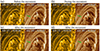 |
Fig. 5. Snapshots from the AIA image sequence. Panel a presents snapshots from the 171 Å channel (left) and from the 193 Å channel (right), before the loop started moving downward in the 171 Å data. The same, but for instances during and after the movement, is shown in panels b–d. The dotted white line in every panel serves as a fiducial marker to highlight the loop displacement in the 171 Å images. In each panel, on top of the 193 Å image, the green and red arrows point to the two separate threads, while the white arrow points to the location where they appear to cross each other (see Sect. 4.1 for details). |
4.2. Heating and cooling
The visibility of a feature in a given AIA passband depends on its temperature and/or density. When we assume that the loop density remains approximately constant during the observation, the intensity fluctuations can then be attributed solely to the change in loop temperature. Therefore, if the loop is visible in the 193 Å channel but not in the 171 Å channel, the reason might be that the loop is too hot to be captured in that particular AIA passband. Conversely, if the loop is present in two passbands at the same time, it may indicate that the loop is either multithermal or that its temperature falls within the response function of both passbands. To understand the evolution of the loop, we examined the intensities at different positions along its length using boxes that covered its lateral extension, as shown in Fig. 6. The light curves from the 211 Å (panel a.2 of Fig. 6), 193 Å (panel b.2), and 171 Å (panel c.2) peak progressively at later times, implying that the loop is cooling (see Appendix C for more details about the cooling time). Interestingly, the shape of the 171 Å curves (panel c.2) is rather steep (near their maxima) compared to the other two channels. Moreover, the vertical dotted line that marks the time when we first observed the downward loop movement in the 171 Å images coincides with the peak of the light curve in panel c.2. This means that the loop starts to cool in the 171 Å channel (rather steeply) at the same time as it starts moving downward. At this point, we cannot determine whether this is more than a coincidence.
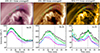 |
Fig. 6. Evolution of the loop intensities in different AIA channels. Panel a.1 shows the time-averaged 211 Å image. The boxes of different colors highlight the locations from which the average intensities (DN s−1) shown in panel a.2 are derived. The same, but for the 193 Å and 171 Å channels, is shown in panels b.1, b.2 and c.1, c.2, respectively. The vertical line in each panel of the bottom row indicates the time stamp at which the loop is first seen to move downward in the 171 Å channel. |
This overarching cooling scenario introduces further complexities to an already complicated evolutionary sequence. Previously, the presence of the loop in 193 Å images and its absence in the 171 Å images (panels b and c of Fig. 2) might have been attributed to a heating event, such as via reconnection. However, this explanation appears less probable now, given the ongoing cooling of the system. Nevertheless, it remains plausible that a localized small-scale heating event did occur at that specific location, but it was undetected in the AIA (and HRIEUV) images.
4.3. Oscillation-induced reconnection
Prior to the detachment of the thin thread, the HRIEUV x-t map (Fig. 2a) displays signatures of transverse oscillations. These oscillations do not exhibit any noticeable change in their amplitude over the two cycles we observed. We fit the observed oscillation as shown in Fig. 7 and calculated that the oscillation period (p) is 2.9 min, and the amplitude (a) is 0.2 Mm. These parameters are similar to typical decayless kink oscillations that are found in active region loops, as reported in Anfinogentov et al. (2015) and Mandal et al. (2022). Curiously, even after the small thread was detached, the parent loop continued to oscillate. This aspect suggests that the transverse oscillation and thread detachment are separate and unrelated events. Consequently, it remains speculation at this point whether the oscillations played a role in triggering the downward movement of the loop.
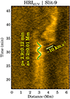 |
Fig. 7. Oscillations in the HRIEUV x-t map. The green curve outlines the fit to the observed transverse oscillations. The derived parameters are shown in the panel. The green line shows the best fit to the slanted ridge above it. The speed, measured through the slope of the dashed line, is also shown in the panel. |
It is indeed a possibility that the observed transverse oscillations have induced reconnection owing to the small-angle misalignment between threads of the loop. As a result, some field lines of the parent loop were pushed sideways, resulting in the appearance of the thread. However, the speed at which the thread moves away (10 km s−1; see Fig. 7) is significantly lower than the typical Alfvén speed (∼1000 km s−1). It is possible, however, that the small-angle misalignment of the field leads to a smaller field component and subsequently lower Alfvén speed. The thin thread therefore is indeed a product of magnetic reconnection because the heat deposited in this case would quickly be distributed throughout the guide field. Further investigations are needed to confirm this hypothesis.
5. Summary and conclusion
Using high-resolution images from HRIEUV ob board Solar Orbiter and AIA on board the SDO, we analyzed the evolution of a coronal loop from two vantage points that were 43° apart. We summarize our main findings below.
Uniform cross-sectional shape and consistency across vantage points. When measured through both HRIEUV and AIA 171 Å images, the width of the loop appears to be similar. This similarity remains consistent throughout the evolution of the loop and along its entire length. These findings suggest that the cross section of the loop is essentially circular. Additionally, it does not support the coronal-veil hypothesis, which predicts that the loop morphology would appear different when viewed from two different perspectives. However, we are aware of the limitations of our dataset, specifically, that the alignment of the two lines of sight (referring to directions, not to the angular difference) is suboptimal. The best-case scenario would involve the two lines of sight lying in a plane perpendicular to the loop plane. However, in the current dataset, both lines of sight roughly align within the loop plane (for the most part), which may mean that it is more difficult to distinguish between the two dimensions of the cross section.
Atypical loop evolution. As seen through HRIEUV, the loop undergoes a unique evolutionary sequence. It initially displays transverse oscillations before a slender thread-like structure detaches from the primary loop. Following this, the main loop also shifts and traverses a distance of about 1.6 Mm within a matter of minutes.
Unknown driving mechanism(s): Currently, the reason(s) for the observed loop evolution remains unclear. Possible scenarios, including projection effects, heating or cooling events, and wave-induced reconnection, do not appear to be the cause in this particular event. Therefore, we require additional information, either from another similar observation or through numerical models, to understand the evolution better.
In conclusion, our study highlights the importance of multiperspective observations in unraveling the complex behaviors of coronal loops. While our findings of unexpected consistency in the loop characteristics from divergent viewing angles challenge the validity of the coronal-veil theory, we cannot make a conclusive statement regarding its applicability (or lack thereof) to all coronal loops. Notably, Malanushenko et al. (2022) also found a mix of veil-like and thin flux-tube-like structures in their work. This highlights the complexity of the problem. A statistical study that includes a variety of loops will be helpful in this regard.
Movie
Movie 1 associated with Fig. 1 Access Supplementary Material
Part of the SolO/EUI Data Release 6.0 (Kraaikamp et al. 2023) and available publicly.
By comparing the location of the second dashed vertical line, it appears that there is a one-pixel shift in the position of the 193 Å loop relative to the 171 Å loop.
It is evident from Fig. 1 that the loop runs diagonally from southeast to northeast with a considerable curvature. Therefore, the two lines of sight are at an angle with the loop plane.
It is obtained at time t2, as indicated in Fig. 3. Nevertheless, the EM values obtained at other times, for example, t1 and t3, are considerably similar.
Acknowledgments
We would like to thank the anonymous referee for providing constructive feedback on the paper. Solar Orbiter is a space mission of international collaboration between ESA and NASA, operated by ESA. The EUI instrument was built by CSL, IAS, MPS, MSSL/UCL, PMOD/WRC, ROB, LCF/IO with funding from the Belgian Federal Science Policy Office (BELSPO/PRODEX PEA 4000112292 and 4000134088); the Centre National d’Etudes Spatiales (CNES); the UK Space Agency (UKSA); the Bundesministerium für Wirtschaft und Energie (BMWi) through the Deutsches Zentrum für Luft- und Raumfahrt (DLR); and the Swiss Space Office (SSO). We are grateful to the ESA SOC and MOC teams for their support. Solar Dynamics Observatory (SDO) is the first mission to be launched for NASA’s Living With a Star (LWS) Program. The data from the SDO/AIA consortium are provided by the Joint Science Operations Center (JSOC) Science Data Processing at Stanford University. L.P.C. gratefully acknowledges funding by the European Union (ERC, ORIGIN, 101039844). Views and opinions expressed are however those of the author(s) only and do not necessarily reflect those of the European Union or the European Research Council. Neither the European Union nor the granting authority can be held responsible for them. The work of JAK was supported by the GSFC Heliophysics Internal Scientist Funding Model competitive work package program.
References
- Anfinogentov, S. A., Nakariakov, V. M., & Nisticò, G. 2015, A&A, 583, A136 [NASA ADS] [CrossRef] [EDP Sciences] [Google Scholar]
- Aschwanden, M. J., Nitta, N. V., Wuelser, J.-P., & Lemen, J. R. 2008a, ApJ, 680, 1477 [NASA ADS] [CrossRef] [Google Scholar]
- Aschwanden, M. J., Wülser, J.-P., Nitta, N. V., & Lemen, J. R. 2008b, ApJ, 679, 827 [NASA ADS] [CrossRef] [Google Scholar]
- Cheung, M. C. M., Boerner, P., Schrijver, C. J., et al. 2015, ApJ, 807, 143 [Google Scholar]
- Chitta, L. P., Peter, H., Parenti, S., et al. 2022, A&A, 667, A166 (SO Nominal Mission Phase SI) [NASA ADS] [CrossRef] [EDP Sciences] [Google Scholar]
- Feng, L., Inhester, B., Solanki, S. K., et al. 2007, ApJ, 671, L205 [NASA ADS] [CrossRef] [Google Scholar]
- Klimchuk, J. A. 2000, Sol. Phys., 193, 53 [NASA ADS] [CrossRef] [Google Scholar]
- Klimchuk, J. A., & DeForest, C. E. 2020, ApJ, 900, 167 [NASA ADS] [CrossRef] [Google Scholar]
- Klimchuk, J. A., Lemen, J. R., Feldman, U., Tsuneta, S., & Uchida, Y. 1992, PASJ, 44, L181 [NASA ADS] [CrossRef] [Google Scholar]
- Klimchuk, J. A., Antiochos, S. K., & Norton, D. 2000, ApJ, 542, 504 [NASA ADS] [CrossRef] [Google Scholar]
- Klimchuk, J. A., Patsourakos, S., & Cargill, P. J. 2008, ApJ, 682, 1351 [Google Scholar]
- Klimchuk, J. A., Knizhnik, K. J., & Uritsky, V. M. 2023, ApJ, 942, 10 [NASA ADS] [CrossRef] [Google Scholar]
- Kraaikamp, E., Gissot, S., Stegen, K., et al. 2023, SolO/EUI Data Release 6.0 2023-01 (Royal Observatory of Belgium (ROB)) [Google Scholar]
- Lemen, J. R., Title, A. M., Akin, D. J., et al. 2012, Sol. Phys., 275, 17 [Google Scholar]
- López Fuentes, M. C., Klimchuk, J. A., & Démoulin, P. 2006, ApJ, 639, 459 [CrossRef] [Google Scholar]
- López Fuentes, M. C., Démoulin, P., & Klimchuk, J. A. 2008, ApJ, 673, 586 [CrossRef] [Google Scholar]
- Malanushenko, A., & Schrijver, C. J. 2013, ApJ, 775, 120 [NASA ADS] [CrossRef] [Google Scholar]
- Malanushenko, A., Cheung, M. C. M., DeForest, C. E., Klimchuk, J. A., & Rempel, M. 2022, ApJ, 927, 1 [NASA ADS] [CrossRef] [Google Scholar]
- Mandal, S., Chitta, L. P., Antolin, P., et al. 2022, A&A, 666, L2 [NASA ADS] [CrossRef] [EDP Sciences] [Google Scholar]
- McCarthy, M. I., Longcope, D. W., & Malanushenko, A. 2021, ApJ, 913, 56 [NASA ADS] [CrossRef] [Google Scholar]
- Müller, D., St. Cyr, O. C., Zouganelis, I., et al. 2020, A&A, 642, A1 [Google Scholar]
- Pesnell, W. D., Thompson, B. J., & Chamberlin, P. C. 2012, Sol. Phys., 275, 3 [Google Scholar]
- Peter, H., & Bingert, S. 2012, A&A, 548, A1 [NASA ADS] [CrossRef] [EDP Sciences] [Google Scholar]
- Plowman, J. E., Kankelborg, C. C., & Longcope, D. W. 2009, ApJ, 706, 108 [NASA ADS] [CrossRef] [Google Scholar]
- Reale, F. 2014, Liv. Rev. Sol. Phys., 11, 4 [Google Scholar]
- Rochus, P., Auchère, F., Berghmans, D., et al. 2020, A&A, 642, A8 [NASA ADS] [CrossRef] [EDP Sciences] [Google Scholar]
- Uritsky, V. M., & Klimchuk, J. A. 2024, ApJ, 961, 222 [NASA ADS] [CrossRef] [Google Scholar]
- Williams, T., Walsh, R. W., & Morgan, H. 2021, ApJ, 919, 47 [NASA ADS] [CrossRef] [Google Scholar]
Appendix A: Context image
In Figure A.1, we provide an overview of the entire field of view (FOV) that is captured by the AIA (shown in panel a) and HRIEUV data (panel b). Figure A.1b shows that the loop on which we focused (indicated by the white rectangle) is situated at a distance from the active region and in close proximity to a dark filament-like structure.
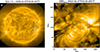 |
Fig. A.1. Full FOVs of the AIA (panel a) and HRIEUV (panel b) datasets. The white rectangle in panel a represents the HRIEUV FOV, and the rectangle in panel b outlines the region in which the loop appears. |
Appendix B: AIA x-t maps
As discussed in Section 4.1, the 193 Å images reveal two loops that are positioned in such a way as to create the illusion of a single structure along the majority of their length. In Figure B.1 we display x-t maps obtained from various slits, illustrating that as they progresses from the loop footpoint toward its apex, the two loops gradually become more distinct and discernible.
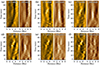 |
Fig. B.1. Further examples of AIA x-t maps. Each panel contains two maps. The left map shows data from 171 Å, and the right map shows data from 193 Å. The slits we used to create these maps are displayed on top of each panel. |
Appendix C: Estimating cooling times
In Section 4.2 we found that the loop cools down gradually over time and that the observed time to cool from 211 Å (emission peaks at t = 10 min) to 171 Å (emission peaks at t = 35 min) is 25 min. We calculate here the theoretical value of the cooling time by estimating the radiative and conductive losses. To do this, we first estimated the electron density as  , where EM is the emission measure, f is the filling factor, and d is the loop diameter. We calculated the EM5 by following the inversion method of Cheung et al. (2015), and the results are presented in Fig. C.1. The average EM value as estimated along the length of the loop is approximately 3×1026 cm−5 at the peak temperature of 2.5 MK (see Fig. C.1g). We set the filling factor (f) to be 1, and the loop diameter (d) was set as 1.6 Mm (see Fig. 3). Using these values, we estimate that the loop density (n) is 1.36×109 cm−3.
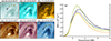 |
Fig. C.1. Emission-measure analysis of the loop. Panels a to f show the loop (outlined by the colored crosses) in six EUV passbands of AIA. The EM curves derived at the locations of these crosses are shown in panel g. |
The radiative cooling time (τr) is calculated as
 (C.1)
(C.1)
where P and T represent the pressure and temperature, and Λ0 is the optically thin radiative loss factor. Using the ideal gas law, P = 2nkT, where k is the Boltzman constant, in Eq. C.1, we obtain
 (C.2)
(C.2)
The values of Λ0 and b were set to 3.53×10⁻¹³ and  , following Eq.3 of Klimchuk et al. (2008).
Next, the conductive cooling time (τc) is calculated as
 (C.3)
(C.3)
where L is the temperature scale length, which is typically taken to be the loop half-length, and κ0 = 10−6. In our case, L≈50 Mm.
Inserting the values of n, L, d, and T from the observation, we arrive at τc = 5.1 × 10³s and τr = 8.5 × 10³s. The total cooling time (τ) from conduction and radiation is expressed as  . Therefore, we obtain τ = 3.1×10³s = 53 min (the observed cooling time is 25 min). Considering the numerous approximations we made to arrive to this value, we conclude that the observed and theoretical values are essentially consistent. The fact that the conductive and radiative cooling times are similar suggests that the loop is in the stage of cooling in which evaporation is transitioning to draining. This is the time of maximum density and minimum density variation. This supports our assumption that a constant density produces the light curves of Fig. 6.
All Figures
|
Fig. 1. Overview of the event. Panel a depicts the relative position of the two spacecraft, SDO and Solar Orbiter, whose data are used in this study. Panel b shows the loop under study in the HRIEUV image, and panels c and d show the same loop, but as seen in the AIA 171 Å and 193 Å channels, respectively. The cyan lines highlight the locations of the artificial slits that are used to generate space-time maps (shown in Figs. 2, 3, 7 and B.1). The arrow in the center of each slit indicates the direction of increasing distance along the slit. The images in panels b–d are unsharp-masked for an improved visibility of the loop. A movie is available online. |
| In the text | |
|
Fig. 2. Representative examples of space-time (x-t) maps derived from the HRIEUV (panel a), AIA 171 Å (panel b), and AIA 193 Å (panel c) image sequences. Zoomed-in versions of these maps, between t = 30 min and 40 min, are presented in panels a.1, b.1, and c.1, respectively. The arrows in these zoomed-in panel point to the slanted ridge that is created by the thin strand. The vertical dotted lines in these panels outline the shift of the loop as judged visually. |
| In the text | |
|
Fig. 3. Comparison of loop widths from HRIEUV and AIA. Panels a and b show x-t maps from HRIEUV and AIA, respectively. The intensity (DN s−1) along the respective colored dashed lines (marked with “t”) is plotted in panels c–e. Panel c shows the derived curves from HRIEUV (green curve) and AIA 171 Å (red) data at t = t3. The curves from t = t2 and t1 are shown in panels d and e, respectively. |
| In the text | |
|
Fig. 4. Variation in the loop width along its length. Panel a shows the normalized HRIEUV intensities calculated along different slits (highlighted via the color bar). The same but for the AIA 171 Å data is shown in panel b. The time at which these loop intensities were derived is identical to the time shown in Fig. 1. Each curve is adjusted to ensure that its peak lies at x = 0 Mm. The vertical and horizontal dotted lines in each panel act as references to approximate the FWHM. AIA curves from slits 5 and 6 are not displayed because the nearby moss-type structure contaminates the curves significantly. |
| In the text | |
|
Fig. 5. Snapshots from the AIA image sequence. Panel a presents snapshots from the 171 Å channel (left) and from the 193 Å channel (right), before the loop started moving downward in the 171 Å data. The same, but for instances during and after the movement, is shown in panels b–d. The dotted white line in every panel serves as a fiducial marker to highlight the loop displacement in the 171 Å images. In each panel, on top of the 193 Å image, the green and red arrows point to the two separate threads, while the white arrow points to the location where they appear to cross each other (see Sect. 4.1 for details). |
| In the text | |
|
Fig. 6. Evolution of the loop intensities in different AIA channels. Panel a.1 shows the time-averaged 211 Å image. The boxes of different colors highlight the locations from which the average intensities (DN s−1) shown in panel a.2 are derived. The same, but for the 193 Å and 171 Å channels, is shown in panels b.1, b.2 and c.1, c.2, respectively. The vertical line in each panel of the bottom row indicates the time stamp at which the loop is first seen to move downward in the 171 Å channel. |
| In the text | |
|
Fig. 7. Oscillations in the HRIEUV x-t map. The green curve outlines the fit to the observed transverse oscillations. The derived parameters are shown in the panel. The green line shows the best fit to the slanted ridge above it. The speed, measured through the slope of the dashed line, is also shown in the panel. |
| In the text | |
|
Fig. A.1. Full FOVs of the AIA (panel a) and HRIEUV (panel b) datasets. The white rectangle in panel a represents the HRIEUV FOV, and the rectangle in panel b outlines the region in which the loop appears. |
| In the text | |
|
Fig. B.1. Further examples of AIA x-t maps. Each panel contains two maps. The left map shows data from 171 Å, and the right map shows data from 193 Å. The slits we used to create these maps are displayed on top of each panel. |
| In the text | |
|
Fig. C.1. Emission-measure analysis of the loop. Panels a to f show the loop (outlined by the colored crosses) in six EUV passbands of AIA. The EM curves derived at the locations of these crosses are shown in panel g. |
| In the text | |
Current usage metrics show cumulative count of Article Views (full-text article views including HTML views, PDF and ePub downloads, according to the available data) and Abstracts Views on Vision4Press platform.
Data correspond to usage on the plateform after 2015. The current usage metrics is available 48-96 hours after online publication and is updated daily on week days.
Initial download of the metrics may take a while.