| Issue |
A&A
Volume 556, August 2013
|
|
|---|---|---|
| Article Number | A50 | |
| Number of page(s) | 13 | |
| Section | The Sun | |
| DOI | https://doi.org/10.1051/0004-6361/201321442 | |
| Published online | 24 July 2013 | |
Global axis shape of magnetic clouds deduced from the distribution of their local axis orientation
1
Observatoire de Paris, LESIA, UMR 8109 (CNRS),
92195
Meudon Principal Cedex,
France
e-mail:
This email address is being protected from spambots. You need JavaScript enabled to view it.
; This email address is being protected from spambots. You need JavaScript enabled to view it.
2
Departamento de Física, Facultad de Ciencias Exactas y Naturales,
Universidad de Buenos Aires, 1428
Buenos Aires,
Argentina
e-mail:
This email address is being protected from spambots. You need JavaScript enabled to view it.
3
Instituto de Astronomía y Física del Espacio,
UBA-CONICET, CC. 67, Suc.
28, 1428
Buenos Aires,
Argentina
Received:
9
March
2013
Accepted:
21
May
2013
Abstract
Context. Coronal mass ejections (CMEs) are routinely tracked with imagers in the interplanetary space, while magnetic clouds (MCs) properties are measured locally by spacecraft. However, both imager and in situ data do not provide any direct estimation of the general flux rope properties.
Aims. The main aim of this study is to constrain the global shape of the flux rope axis from local measurements and to compare the results from in-situ data with imager observations.
Methods. We performed a statistical analysis of the set of MCs observed by WIND spacecraft over 15 years in the vicinity of Earth. We analyzed the correlation between different MC parameters and studied the statistical distributions of the angles defining the local axis orientation. With the hypothesis of having a sample of MCs with a uniform distribution of spacecraft crossing along their axis, we show that a mean axis shape can be derived from the distribution of the axis orientation. As a complement, while heliospheric imagers do not typically observe MCs but only their sheath region, we analyze one event where the flux rope axis can be estimated from the STEREO imagers.
Results. From the analysis of a set of theoretical models, we show that the distribution of the local axis orientation is strongly affected by the overall axis shape. Next, we derive the mean axis shape from the integration of the observed orientation distribution. This shape is robust because it is mostly determined from the overall shape of the distribution. Moreover, we find no dependence on the flux rope inclination on the ecliptic. Finally, the derived shape is fully consistent with the one derived from heliospheric imager observations of the June 2008 event.
Conclusions. We have derived a mean shape of MC axis that only depends on one free parameter, the angular separation of the legs (as viewed from the Sun). This mean shape can be used in various contexts, such as studies of high-energy particles or space weather forecasts.
Key words: Sun: coronal mass ejections (CMEs) / Sun: heliosphere / magnetic fields / solar-terrestrial relations
© ESO, 2013
1. Introduction
Coronal magnetic configurations are frequently unstable and lead to coronal mass ejections (CMEs) propagating into interplanetary space (see the reviews of Pick et al. 2006; Kleimann 2012). Evidence of the presence of a twisted flux tube, or flux rope, had been reported before the launch and especially during the time when the CME took off (Canou et al. 2009; Guo et al. 2010; Cheng et al. 2011, 2013; Patsourakos et al. 2013). The magnetohydrodynamic (MHD) models of CMEs commonly include a flux rope (e.g. Forbes et al. 2006; Aulanier et al. 2012; Schmieder et al. 2013, and references therein). Coronagraph observations visualize the denser regions of CMEs through the Thomson scattering of white light by free electrons (see Howard 2011; Thernisien et al. 2011, for reviews). These observations are compatible with a flux rope topology with an appearance that depends on the relative orientation of the flux rope with the line of sight (e.g. Cremades & Bothmer 2004). An approach was developed with a forward model having a dense shell around a flux rope-like shape and fitted visually to coronagraph images of CMEs (Thernisien et al. 2006; Krall 2007; Thernisien 2011, and references therein). This method was developed to incorporate the two views from the Solar Terrestrial Relations Observatory (STEREO) spacecraft (Wood et al. 2009, 2011). These advances were also supported by important developments of MHD simulations of flux rope propagation, as reviewed by Lugaz & Roussev (2011).
Magnetic clouds (MCs) are detected within a fraction of interplanetary CMEs (Wimmer-Schweingruber et al. 2006, and references therein). Their main characteristic is a large and smooth rotation of the magnetic field direction. This signature is classically interpreted as the presence of a twisted magnetic flux tube, simply called a flux rope (e.g. Lepping et al. 1990; Burlaga 1995, and references therein). However, the in situ observations alone are not sufficient to firmly conclude that a flux rope configuration is the only possibility (Al-Haddad et al. 2011), but combining in situ, coronagraphic observations and forward modeling (Krall 2007) enforces the possibility that there is a flux rope in all CMEs (Xie et al. 2013).
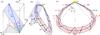 |
Fig. 1 Definitions of the angles and flux-rope geometry. a) Schema defining the
angles of the local MC axis direction. It is a local view of panel b).
The unit vector |

The magnetic field and plasma measurements are only available along the spacecraft trajectory during the MC crossing. Then, various magnetic models can be proposed to gain information on the flux rope cross section. Their free parameters are determined by a least square fit to the magnetic data obtained from the in situ observations. Such models can then provide the magnetic field distribution within the cross section, as well as the local axis orientation of the flux rope. The simplest and most used model is the cylindrical linear force-free field model, which is also referred to as the Lundquist model (see e.g. Goldstein 1983; Lepping et al. 1990; Leitner et al. 2007). Extensions to a non-circular cross-section (e.g. Vandas & Romashets 2003; Démoulin & Dasso 2009), or non-force-free models (e.g. Mulligan et al. 1999; Mulligan & Russell 2001; Hidalgo 2011) have been proposed without, so far, a model emerging as a standard for MCs. An alternative is to solve the magneto-hydrostatic equations in the MC frame with the magnetic data as boundary conditions for the integration procedure and with the hypothesis of local invariance along the axis. In such a model, the theoretical constraint that the plasma and axial field pressure should only depend on the magnetic flux function in the cross section is used to determine the local axis direction (e.g. Hu & Sonnerup 2002; Sonnerup et al. 2006; Isavnin et al. 2011). To summarize, all these approaches provide a magnetic model of the flux rope cross section with a local invariance along the axis.
An extension of the approaches presented above has been proposed with several models developed to incorporate the curvature of the flux rope axis with a toroidal geometry (keeping an invariance along the axis, e.g., Marubashi 1997; Romashets & Vandas 2003; Marubashi & Lepping 2007; Romashets & Vandas 2009). This is especially needed when the angle between the spacecraft trajectory and the local axis direction is small (e.g. Marubashi et al. 2012; Owens et al. 2012). Including the toroidal geometry implies a larger number of free parameters for the model, and it has not yet been demonstrated how well the data from a single spacecraft can constrain all of them, in particular the local curvature of the axis that is important for obtaining the global axis shape of the flux rope axis. This approach would benefit from well-separated spacecraft since data from only two spacecraft provide more constraints on the toroidal model (Nakagawa & Matsuoka 2010).
However, although multispacecraft observations can provide a more complete set of data to analyze a flux rope configuration, there is only a very limited number of MCs that have been sampled along the flux rope by at least two spacecraft (see Kilpua et al. 2011, for a review). When the two spacecraft are separated with a significant angle (several 10° as seen from the Sun), the data can roughly estimate the extension of the flux rope (Mulligan & Russell 2001; Reisenfeld et al. 2003). Then, tighter constraints require more spacecraft, but only very few MCs have been observed by at least three spacecraft crossing the flux rope close enough to its axis. When possible, such cases allow the local determination of its axis orientation at distant regions along the axis if the spacecraft are sufficiently separated (Farrugia et al. 2011; Ruffenach et al. 2012). Still, it remains unclear whether the different methods used to determine the axis orientation (see above) have a large scatter/bias or if the flux rope axis has a more complex shape than typically proposed (compare Fig. 1c to Fig. 12 of Farrugia et al. 2011). Finally, the case studied by Burlaga et al. (1981), with an MC scanned by four spacecraft, remains an exceptional case from which the flux rope shape was constrained (see their Fig. 5). The occurrence of correlated observations therefore remains too scarce to derive mean global properties of the flux rope in MCs from such studies.
On the other hand, several types of studies require a more general view of the flux rope structure. An example is the understanding of the crucial role played by the field line length in the time delay observed between particles of different energies during the propagation of high-energy particles within MCs (e.g. Larson et al. 1997; Masson et al. 2012). Another example is the study aiming at relating the flux rope properties to the 3D configuration of its solar source in a more complete way than with timing, orientation, and magnetic flux (e.g. as realized in Nakwacki et al. 2011, and references therein). So far, simplified methods have been developed to get estimations of some general MHD quantities contained in MCs, such as magnetic helicity (Dasso et al. 2003, 2006; Dasso 2009) or magnetic energy (Nakwacki et al. 2011). They modeled the local flux tube of the cloud given from in situ observations. However, a proper model of the global magnetic cloud shape will help improve their quantification.
Determination of the 3D shape of an MC would need many spacecraft to sample it at as many locations as possible. Since the cost is prohibitory, could we not instead combine the information obtained from many MCs to derive a mean global configuration of MCs? Supposing a simply curved axis, the flux rope axis direction provides an indication of the location where the flux rope is crossed by the spacecraft (Fig. 1c). For example, an axis orthogonal to the radial direction (Sun-spacecraft) would mean that the flux rope is crossed at its apex (or nose), while a local axis more oriented in the radial direction would imply that the crossing is farther away from the apex. Then, observations of many MCs with various deduced local axis directions can sample flux ropes along their axis.
In this study, we further analyze the above property to derive a mean axis shape for the set of studied MCs. This is done in three main steps. First, in Sect. 2, we analyze the statistical properties of the set of MCs, testing the correlation between the MC parameters. We derive the statistical distributions of the axis orientation parameters and test their robustness using various selection criteria on the MC parameters. Second, in Sect. 3, we use an axis model to investigate the effect of the overall axis shape on the distribution of the local axis orientation. Then, in Sect. 4, we present the reverse procedure by deducing the mean global axis shape from the observed distribution of the local axis orientation. These results are complemented in Sect. 5 by our analysis of a well-observed event where the flux rope extension and its axis can be constrained by heliospheric images and in situ data. Here, we compare the axis shape deduced from the imager data with our results from the in situ data of an MC set. Finally, in Sect. 6, we summarize our results and draw conclusions about their implications.
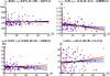 |
Fig. 2 Properties of MCs observed at 1 AU versus the location angle (λ in degree). The correlations are shown for the mean MC velocity (V in km s-1), the MC radius (R in AU), the axial magnetic field strength (B0 in nT), and the axis inclination (i in degree) for the full set of MCs. λ > 0 and λ < 0 are shown in red and blue, respectively, and the abscissa, |λ|, allows comparing the two leg sides of the flux rope (Fig. 1c). The straight lines are linear fits to the data points (MCs) showing the tendency. The results with the total MC set are shown in black (linear fit and top labels). cP and cS are the Pearson and Spearman rank correlation coefficients, respectively, and “fit” is the least-square fit of a straight line (in black) to the full data set. |
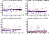 |
Fig. 3 Properties of MCs observed at 1 AU versus the axis inclination on the ecliptic (i in degree). The correlations are shown for the mean MC velocity (V in km s-1), the MC radius (R in AU), the axial magnetic field strength (B0 in nT), and the asymmetry factor (asf in %) for the full set of MCs. The asymmetry factor (asf, see Lepping et al. 2005) measures twice the time difference between the middle of the MC time interval and the closest approach (“center time”). It is expressed in % of the MC event duration. It has been introduced to measure how far in time the peak in the modeled magnetic field is from the midpoint of observed MC. The drawing convention is the same as in Fig. 2. |
2. Observations
2.1. Set of observed MCs
We first summarize the list of MCs as defined by Lepping et al. (1990). They first identified the time intervals as having the four characteristics of MCs in the WIND data (defined by Burlaga et al. 1981). Then, they determined the MC boundaries with the jumps in the plasma and magnetic field measurements, and they fitted the magnetic field in the selected time intervals with a flux rope model. This model assumes a linear force-free, or constant-α, magnetic field (Lundquist 1950). The least square fit to the in situ data determines seven parameters of the model: (1) the longitude (φ) and (2) the latitude (θ) of the flux rope axis (see Sect. 2.2); (3) the distance of the spacecraft from the flux rope axis at closest approach point (Y0); (4) the magnetic field strength on the flux rope axis (B0); (5) the twist (α); (6) the sign of the magnetic helicity (H = ± 1); and (7) the time at closest approach to the flux rope axis (t0). The mean velocity (V) of the MC is directly determined from the measured proton velocity. From these parameters, other physical quantities of the flux rope are computed, such as the flux rope radius (R) and the impact parameter (p = Y0/R).
In the present study, we use an extended list of events (Table 21), which is based on the results of Lepping & Wu (2010) and includes more recent MCs. This list, on the date of February 13, 2013, contains the parameters obtained for 121 MCs observed near Earth by WIND spacecraft from February 1995 to December 2009. However, when removing the cases where the handedness could not be determined (flag f in the list) or the fitting convergence could not be achieved (flag F), this list is restricted to 111 MCs. Within the remaining cases, four MCs have an impact parameter p > 1 (so a fitted flux rope extending beyond the first zero of the axial field in the Lundquist model). Removing these suspicious cases, all of the worse class (quality 3, where the quality is defined in Lepping et al. 1990 according to the χ2 value of the fit of a flux rope model to data), 107 MCs remain, ranging from quality 1 to quality 3.
2.2. Definition of the axis orientation
The WIND data are defined in the geocentric solar ecliptic (GSE) system of reference
(with unit vectors  ,
ŷGSE, ẑGSE), where
points from the Earth toward the Sun, ŷGSE is in the ecliptic
plane and in the direction opposite to the planetary motion, and
ẑGSE points to the north pole. The flux rope axis orientation is
classically defined in spherical coordinates by two angles: the longitude
(φ) and the latitude (θ) as shown in Fig. 1a. The polar axis of the spherical coordinates
(θ ≈ 90°) is singular since it corresponds to any values of
φ. The above choice for a reference system sets this axis along
zGSE which is both a possible and a nonspecific axis
direction. Therefore, the coordinates (φ,θ) are not appropriate for
studying the correlation of MC properties with φ, as we would need to
limit the study to low | θ | values to have meaningful φ
values.
,
ŷGSE, ẑGSE), where
points from the Earth toward the Sun, ŷGSE is in the ecliptic
plane and in the direction opposite to the planetary motion, and
ẑGSE points to the north pole. The flux rope axis orientation is
classically defined in spherical coordinates by two angles: the longitude
(φ) and the latitude (θ) as shown in Fig. 1a. The polar axis of the spherical coordinates
(θ ≈ 90°) is singular since it corresponds to any values of
φ. The above choice for a reference system sets this axis along
zGSE which is both a possible and a nonspecific axis
direction. Therefore, the coordinates (φ,θ) are not appropriate for
studying the correlation of MC properties with φ, as we would need to
limit the study to low | θ | values to have meaningful φ
values.
The Earth-Sun direction is a particular one considering the encounter of MCs coming from the Sun by a spacecraft. We then set a new spherical coordinate system with its polar axis along xGSE (Fig. 1a). Since this direction corresponds in theory to the spacecraft crossing the flux rope parallel to the legs, and since in practice it is not possible to detect flux rope legs (e.g., the magnetic field rotation is very difficult to detect in the partial and longterm crossing of a leg), this direction does not appear in the MC data set studied here. Then, we define the inclination on the ecliptic (i) and the location (λ) angles (Fig. 1). The names for these angles are derived from an MC with an axis located in a plane and with the distance to the Sun increasing along the flux rope from any of its legs to its apex (as shown in Fig. 1c). The angle i is the inclination of this plane (in light blue) on the ecliptic (in light gray) as shown in Figs. 1a,b. The angle λ is evolving monotonously along the flux rope, implicitly marking the location where the spacecraft intercepts the flux rope (Fig. 1c). It defines the position of the spacecraft crossing explicitly if the axis shape is known.
As for the latitude angle θ, the inclination angle i is
defined in the interval [−90°,90°] with
i = 0 when the MC axis is in the ecliptic plane (corresponding to
θ = 0). The angle λ is measured from the plane
(ŷGSE,ẑGSE) towards the
MC axis (Fig. 1a). In contrast, the cone angle
βA was defined from
towards the MC axis (e.g. Lepping et al. 1990).
These angles are simply linked by
λ = 90°−βA. At the MC apex,
βA ≈ 90°, while the MC legs have
βA ≈ 0° or 180°. It implies that
βA is not a convenient angle to compare results on both
sides of the apex since the data cannot be reported on the same abscissa. However,
choosing λ in [−90°,90°]
allows us to do so, as it is shown by blue and red dots in Fig. 2.This is why we introduce the location angle as a continuously changing
quantity: from λ ≈ −90° in one leg, to
λ ≈ 0° at the apex, to λ ≈ 90°
in the other leg for a flux rope axis having a curvature always directed inward (as in
Fig. 1c). With this definition of λ,
the properties of both legs are simply compared by using |λ |. Next, if
the flux rope is not north-south oriented (e.g. with a plane close to the ecliptic plane),
then λ > 0 in the east leg and
λ < 0 in the west leg (Fig. 1c). In the case of a flux rope more north-south oriented
(inclined with the ecliptic plane), then λ > 0
and λ < 0 correspond respectively to the northern
and southern legs for i > 0 (and the reverse for
i < 0).
The relations between (i,λ) and (φ,θ) are simply:
 where
we include the absolute value of sinφ since i evolves
similarly as θ.
where
we include the absolute value of sinφ since i evolves
similarly as θ.
2.3. Statistical properties of the axis orientation
We analyze the correlations of the local axis orientation parameters below with the other MC parameters deduced from the Lundquist model for the set of 107 MCs. The correlation analysis allows us to obtain proper sets of data to study the distribution of the local axis orientation parameters.
We present some of the correlation analysis results for the location angle λ in Fig. 2, and we find that λ only weakly correlates with the other MC parameters (apart for φ and θ since the correlation is present from the definition, Eq. (1)). A general result is also that there is no significant difference between both legs (i.e. λ > 0 and λ < 0 as defined in Fig. 2), so that in the following we only describe correlations with |λ|. For the full set of MCs, the strongest correlation is obtained with the flux rope radius R (Fig. 2, top right). Still, this correlation is quite weak regarding both the Pearson and Spearman rank correlation coefficients (cP = −0.29, cS = −0.24). Moreover, this correlation is even weaker (cP = cS = −0.12) if we limit the analysis to a set with the best and good cases (qualities 1 and 2 as defined by Lepping et al. 1990), i.e., 74 MCs. The next significant correlation is with the impact parameter (not presented here, with cP = 0.2, cS = 0.13), but this weak correlation almost vanishes for a set with only quality 1 and 2 MCs (cP ≈ cS ≈ −0.03). Then, the next strongest correlation is between | i | and |λ| (Fig. 2, bottom right), and this weak correlation is kept with the quality 1 and 2 MC set. The other MC parameters show no significant correlation with λ, e.g., for V and B0 (Fig. 2).
The inclination angle, i, has an even lower correlation with the other MC parameters than with λ (Fig. 3). Very similar results are obtained with the sets i > 0 and i < 0 (by comparing red and blue points and lines in Fig. 3). The best correlation is found with the MC velocity, V. Still, it is a very weak correlation (cP = 0.13, cS = 0.12). To confirm the above results that present very weak correlations between λ, i, and the other MC parameters, we went on to investigate the correlations obtained by ordering first the full MC set by increasing value of one MC parameter (such as V, R, B0, and more generally all the parameters reported in the table of Lepping & Wu 2010). Then, we computed the mean value of i in subsets of MCs, scanning increasing values of the selected parameter. This analysis (not presented here) confirmed that there is no significant dependence of i on any of the other MC parameters (apart with θ and φ because of the definition, Eq. (2)). The present results for λ and i imply that the MC properties are statistically independent of the axis orientation around the Sun-Earth line, as far as the limited number of MCs studied allows us to conclude.
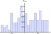 |
Fig. 4 Probability distribution, |


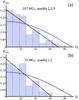 |
Fig. 5 Probability distribution, |
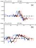 |
Fig. 6 Property of the probability distribution |
2.4. Distributions of the axis orientation
The probability distribution of the axis inclination i, presented in Fig. 4, is broad with flux ropes detected in all ranges of i, from [−90°,90°]. The main maxima is for flux ropes oriented close to the ecliptic plane, and there are secondary maxima for | i| ≈ 50°. There is also a marked difference with the sign of i: the cases with i > 0 are nearly evenly distributed (within the statistical fluctuations) compared to those with i < 0. Altogether, this implies that the flux rope inclination on the ecliptic is broadly distributed without a single privileged direction.
In contrast, the probability distribution of λ (Fig. 5) is strongly nonuniform with a probability decreasing rapidly with growing |λ|. Marubashi (1997) mentioned the possibility of finding the direction of the flux-rope legs following the Archimedean spiral. From numerical simulations, Vandas et al. (2002) find a similar trend, finding evidence of an orientation of the legs similar to the solar wind Parker spiral. However, similar distributions are obtained for λ > 0 and λ < 0 (not shown) within the limit of statistical fluctuations, in particular for higher |λ| values (corresponding to MC legs where few MCs are detected). Restricting the MC set to the qualities 1 and 2, so to 74 MCs, removes all the high |λ| values (Fig. 5b). It implies a distribution that is more peaked at low |λ| values.
The cases with large |λ| correspond to the spacecraft crossing the region of a MC leg. These cases typically lead to the largest uncertainty of the fitted flux rope parameters (e.g. Lepping & Wu 2010) because of the difficulties in fitting a Lundquist model to the data. They are observed in the regions of the MC legs, and changing their locations in the distribution tail only weakly modifies the global distribution. As such, we consider the whole distribution of λ without truncating it. As shown in Fig. 5, a much stronger effect is present by selecting the MCs with the quality class. Moreover, the low number of cases in the distribution tail implies that the λ distribution has large statistical fluctuations for high |λ| values.
We study the probability distributions of λ further by fitting them with
a straight line (Fig. 5) to decrease the statistical
fluctuations. The slope of the line, or simply slope of
 ,
is directly linked to the mean of the distribution ⟨ |λ| ⟩ (see Eq.
(15) and related text in Démoulin et al. 2013).
Since the statistical fluctuations of the mean value of |λ| are on the
order of
,
is directly linked to the mean of the distribution ⟨ |λ| ⟩ (see Eq.
(15) and related text in Démoulin et al. 2013).
Since the statistical fluctuations of the mean value of |λ| are on the
order of  ,
where N is the number of MCs in the distribution, this fitting procedure
allows us to split the MC data set in subsets while still keeping relatively low
statistical fluctuations on the slope (see Fig. 6).
It implies that we can test whether the probability distribution of |λ|
is affected by some of the other MCs parameters. To do so, we first order the MCs by a
growing order of one selected parameter, and we then fit
for each subset of N MCs, progressively shifting to higher values of the
selected MC parameter (by step of one MC). This allows the study of the slope evolution of
the fit versus the selected parameter.
,
where N is the number of MCs in the distribution, this fitting procedure
allows us to split the MC data set in subsets while still keeping relatively low
statistical fluctuations on the slope (see Fig. 6).
It implies that we can test whether the probability distribution of |λ|
is affected by some of the other MCs parameters. To do so, we first order the MCs by a
growing order of one selected parameter, and we then fit
for each subset of N MCs, progressively shifting to higher values of the
selected MC parameter (by step of one MC). This allows the study of the slope evolution of
the fit versus the selected parameter.
We find no significant dependence of the slope of
on any of the other MC parameters except a weak one with the flux rope radius that we show
in Fig. 6a for subsets of N = 20
MCs. Indeed, the smaller MCs (R < 0.1 AU) have a
slightly weaker slope, since they have a broader
than the larger MCs. A fluctuation of the slope of similar amplitude is also found when
the MCs are ordered with | i |. Still, there is no significant slope
difference between the MCs that are more parallel to the ecliptic (say
| i| < 20°) from those more
inclined on it. We conclude that the probability distribution
is almost independent of the orientation of the flux rope, as well as of other MC
parameters (not shown), except for the weak dependence on R.
The probability distribution of λ is closely linked to the mean shape of the axis (Fig. 1c). For example, with a circular shape and relatively close legs (separated by an angle of less than few 10°), the expected λ distribution is fcos = ccos|λ | (where c is a constant for normalizing the total probability to 1), as is shown and discussed in detail in Sect. 3.3. The fit of fcos to the observed distribution, as shown in Fig. 5 (blue curve), indicates that fcos is too broad a distribution compared to the observed one. This difference is even stronger in the case where only the MCs of qualities 1 and 2 are considered. This already implies that the axis shape is flatter than a circular one.
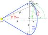 |
Fig. 7 Diagram defining a model of the flux rope axis with an elliptical shape. The legs are represented by straight and radial segments tangent to the ellipse and linking it to the Sun. ϕ is the angle of the cylindrical coordinates (ρ,ϕ). The point C is the ellipse center and M is the point of interest (where the spacecraft crosses the flux rope). |
3. Simple models of a global flux-rope axis
Since the derivation of the mean shape of the axis from
is not fully straightforward, we analyze the reverse problem in this section, i.e. computing
the location angle distribution from given models of the global axis shape. In particular,
how sensitive is the λ probability distribution to the global axis shape
and what are the main axis geometry parameters affecting the distribution?
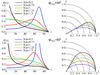 |
Fig. 8 Probability distribution of the location angle λ (left
panels) and the corresponding axis shape (right panels)
for the elliptical model of the flux rope axis (defined in Fig. 7). Since the model is symmetric,
|

3.1. Axis model with an elliptical shape
We select a flux rope model that has enough free parameters to describe a wide variety of axis shapes, but which also has the minimum of complexity needed. The flux rope axis is supposed to be planar, and it is described by a portion of an ellipse, up to the points T and T’, where the tangent to the ellipse is a radial segment attached to the Sun (Fig. 7). These straight segments simply describe the flux-rope legs and link the flux rope to the Sun. As such, the ellipse is not directly attached to the Sun as in Krall 2007 among others. The in situ measurements in a region within the flux rope legs with λ ≈ 90° do not show any important rotation of the magnetic field, while the spacecraft crosses the MC. As such, these events are typically not reported as MCs (Owens et al. 2012, and references therein). Similarly here, we do not consider the straight parts of the axis model in the computed distributions of location angles λ.
The ellipse center, C, is at a distance d from the Sun, and its axes are
along the radial and ortho-radial directions with half size a and
b, respectively (Fig. 7). A point
M on the elliptical part of the axis is at a distance ρ from the Sun:
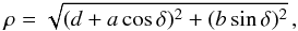 (3)where δ
is the angle defining the position of M from the ellipse center. The other cylindrical
coordinate of M, ϕ, is given by
(3)where δ
is the angle defining the position of M from the ellipse center. The other cylindrical
coordinate of M, ϕ, is given by  (4)The angle between
the tangent to the ellipse at M and the local ortho-radial direction from the Sun is the
location angle λ (Fig. 7). It is
related to the other angles and ellipse parameters by
(4)The angle between
the tangent to the ellipse at M and the local ortho-radial direction from the Sun is the
location angle λ (Fig. 7). It is
related to the other angles and ellipse parameters by 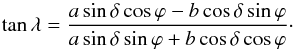 (5)The above
equation is simplified by the introduction of the angle u defined as
(5)The above
equation is simplified by the introduction of the angle u defined as
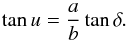 (6)Then, Eq. (5) simplifies to
  (7)with
λ within the interval
[−90°,90°]. This equation implicitly
expresses the angle λ in function of ϕ and the
parameters (a,b,d) after eliminating u with Eq. (6) and δ with Eq. (4) (i.e. expressing cosδ in
function of tanϕ).
(7)with
λ within the interval
[−90°,90°]. This equation implicitly
expresses the angle λ in function of ϕ and the
parameters (a,b,d) after eliminating u with Eq. (6) and δ with Eq. (4) (i.e. expressing cosδ in
function of tanϕ).
In summary, this elliptical model of the axis depends on three parameters:
{ a,b,d }. Equivalently, it is also defined by these three other
parameters:
{ a + d,b/a,ϕmax }
representing the apex distance from the Sun, the aspect ratio, and the maximum angular
extension, respectively, defined by: 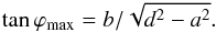 (8)
(8)
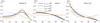 |
Fig. 9 Comparison of the probability distribution of the location angle λ for the elliptical model of the flux rope axis with a given aspect ratio b/a in each panel (see Fig. 7). The distributions are normalized as in Fig. 8 and the dotted curve is the distribution for a small circular front. The maximum extension angle ϕmax only has a weak effect on the distribution shape compared to the strong effect of the aspect ratio b/a. |
3.2. Probability distribution of the location angle λ
The in situ observation of an MC made from a single spacecraft only provides a local estimation of the flux rope axis orientation (by fitting a flux rope model to the magnetic field data). For a given MC, only one value of λ is thus available, say at point M along the flux rope axis (Fig. 7). We first consider a series of flux ropes contained in the ecliptic plane (i.e. i ≈ 0). On the time scale of a solar cycle, the Sun launches MCs from any longitude. Moreover, since the Sun is rotating, any privileged active longitude is covered on a time scale of ~11 years. It implies that MCs are expected to be observed with an equiprobability of ϕ, except for an expected lower rate of detection in the legs owing to an observational bias. Since the flux rope is only partially crossed, it is not always detected (e.g. Owens et al. 2012, and references therein).
We have shown in Fig. 4 that a large fraction of flux ropes is significantly inclined with respect to the ecliptic plane. However, since we find no significant correlation between any of the estimated flux rope characteristics and the angle i (Sect. 2.3), it is reasonable to expect an equiprobable distribution of ϕ for any i angle. Moreover, the probability distribution of |λ| remains similarly peaked towards low |λ|, with a mean slope almost independent of | i | (Fig. 6b). We deduce that the range of solar-latitude launches is broad enough to allow a similar scan of the flux-rope axis with significant | i | values as the ones with low | i | values.
We then suppose that the probability of ϕ,
 ,
is uniform within the set of detected MCs and for the above axis model, at least away from
the legs. With ϕ in the interval
[−ϕmax,ϕmax],
the distribution
is simply a constant defined by the normalization of the total probability to unity:
,
is uniform within the set of detected MCs and for the above axis model, at least away from
the legs. With ϕ in the interval
[−ϕmax,ϕmax],
the distribution
is simply a constant defined by the normalization of the total probability to unity:
 (9)For flux ropes
having an axis curved inward, as in Fig. 7, there is
a monotonous relationship between λ and ϕ. Considering
that the intervals [ϕ,ϕ + dϕ] and
[λ,λ + dλ] contain the same number of cases, we link
the two probabilities
(9)For flux ropes
having an axis curved inward, as in Fig. 7, there is
a monotonous relationship between λ and ϕ. Considering
that the intervals [ϕ,ϕ + dϕ] and
[λ,λ + dλ] contain the same number of cases, we link
the two probabilities  and
by
and
by  (10)With
known and dϕ/dλ computed from the
equations of the above axis model, Eq. (10)
provides the probability distribution of λ, which can be compared with
the observed ones (Fig. 5).
(10)With
known and dϕ/dλ computed from the
equations of the above axis model, Eq. (10)
provides the probability distribution of λ, which can be compared with
the observed ones (Fig. 5).
The computation of dϕ/dλ is realized
by differentiating Eqs. (4), (6), and (7). Regrouping these equations provides 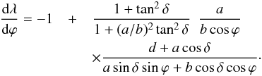 (11)Then,
is computed from Eqs. (9)–(11).
(11)Then,
is computed from Eqs. (9)–(11).
3.3. Particular probability distributions of λ
The probability
has a simple expression at the apex (where λ = 0,
ρ = ρmax = a + d,
and ϕ = 0)  (12)After introducing the
radius of curvature of the ellipse,
Rc = b2/a,
at ϕ = 0, Eq. (12) is
rewritten as
(12)After introducing the
radius of curvature of the ellipse,
Rc = b2/a,
at ϕ = 0, Eq. (12) is
rewritten as  (13)It shows that
becomes singular (infinite) at the apex when
Rc = ρmax, that is, when the
ellipse is tangential to the circle ρ = ρmax,
so that the front is locally the flattest possible (in cylindrical coordinates). The black
solid curves in Fig. 8 illustrate cases with
Rc very close to ρmax. The left
hand panels show the probability distributions that become infinite for
λ → 0° (apex) for
ϕmax = 30° and 60°, while the right
hand panels show the half ellipse shape following the circle
ρ = ρmax near the apex (especially the case
ϕmax = 60°). Other cases with
Rc close to ρmax (i.e. pink
solid curves in Fig. 8) show that the corresponding
probability
is much more peaked at λ = 0 than the probability deduced from
observations (Fig. 5), even if we include the same
binning (not shown).
(13)It shows that
becomes singular (infinite) at the apex when
Rc = ρmax, that is, when the
ellipse is tangential to the circle ρ = ρmax,
so that the front is locally the flattest possible (in cylindrical coordinates). The black
solid curves in Fig. 8 illustrate cases with
Rc very close to ρmax. The left
hand panels show the probability distributions that become infinite for
λ → 0° (apex) for
ϕmax = 30° and 60°, while the right
hand panels show the half ellipse shape following the circle
ρ = ρmax near the apex (especially the case
ϕmax = 60°). Other cases with
Rc close to ρmax (i.e. pink
solid curves in Fig. 8) show that the corresponding
probability
is much more peaked at λ = 0 than the probability deduced from
observations (Fig. 5), even if we include the same
binning (not shown).
The expression of the probability
can also be simplified in the limit of a circular front, that is, when
b = a, as  (14)This result shows that
for a narrow angular extension, that is,
a/d ≪ 1 or equivalently
ϕmax ≪ 90°,
simply has a cosλ dependence. Such
is more extended in λ compared with observations (see the blue curves in
Fig. 5). In contrast, for a broad angular extension
(a = d or
ϕmax = 90°, using Eq. (8)),
is uniform in λ and
(14)This result shows that
for a narrow angular extension, that is,
a/d ≪ 1 or equivalently
ϕmax ≪ 90°,
simply has a cosλ dependence. Such
is more extended in λ compared with observations (see the blue curves in
Fig. 5). In contrast, for a broad angular extension
(a = d or
ϕmax = 90°, using Eq. (8)),
is uniform in λ and  .
This case corresponds to an axis located on a circle attached to the Sun (so without the
straight segments departing from T and T’ in Fig. 7).
Such a distribution is also incompatible with the distribution deduced from the
observations (Fig. 5).
.
This case corresponds to an axis located on a circle attached to the Sun (so without the
straight segments departing from T and T’ in Fig. 7).
Such a distribution is also incompatible with the distribution deduced from the
observations (Fig. 5).
3.4. Expected probability distributions of λ
The elliptical model of the axis shown in Fig. 7 has
three free parameters: a,b, and d. We fix the general
scale of the model by normalizing the sizes by ρmax, i.e.
fixing a + d = 1. We explore below the effect of the
aspect ratio b/a and
ϕmax on ,
setting
to a uniform distribution. The aim is to compare the variety of the computed distributions
with the observed ones (Fig. 5).
For a given ϕmax value, the aspect ratio
b/a has an important effect on
as shown in Fig. 8. For
b/a = 1 (green curve),
corresponding to a circular shape of the flux rope axis,
is close to a cosλ function except when ϕmax
is getting close to 90°, in agreement with Eq. (14). Since b/a is
slightly lower than 1,
deviates significantly from the cosλ function with a peak appearing in
the leg part (more precisely around λ ≈ 60–70° for the blue
and red curves) and growing rapidly as
b/a decreases. In parallel, a large
decrease in
is present for λ ≤ 50°, therefore for a region near the apex
region. In contrast, increasing b/a
above 1 increases sharply the probability in the apex region at the expense of the leg
region (pink and black curves, Fig. 8).
The above effect of b/a is enhanced
for larger ϕmax (lower panels of Fig. 8). However, the effect of ϕmax is much
lower than the effect of b/a as shown
in Fig. 9. Indeed,
b/a is the main parameter that
defines the shape of
with the presence of a peak in the leg region for
b/a < 1 and
at the apex for
b/a > 1.
ϕmax only weakly modulates this main tendency and it has a
significant effect on
only for ϕmax close to 90° (so for an axis shape
close to an ellipse directly attached to the Sun).
The comparison of the results for the distribution shown in Figs. 8 and 9 with those obtained for the
observations and shown in Fig. 5 reveals that the
observed λ probability distribution sets stringent conditions for a
global flux rope axis model. The axis shape needs to be flatter than a circular shape, but
it cannot be too flat. In particular, an aspect ratio
b/a of only 1.25 (Fig. 9) implies an already too peaked
distribution around the apex compared to Fig. 5.
We conclude that, within the hypothesis of a uniform
distribution and comparable axis shape for MCs, the observed distribution
sets a stringent constrains on the mean axis shape.
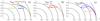 |
Fig. 10 Mean flux-rope axis deduced from the probability distribution
|
4. Deduction of the axis shape from the data
The forward modeling presented in Sect. 3 has
emphasized the relationship between the shape of the flux rope axis and the expected
probability distribution .
It specifies qualitatively which kind of axis shapes are closer to observations. However
there are still significant differences between the modeled
distributions (Figs. 8 and 9) and the observed ones (Fig. 5).
Rather than finding the optimum values of
b/a and
ϕmax of the elliptic model that best fit the observed
distributions, we derive a procedure below for obtaining the axis shape from the observed
distributions.
4.1. Method
Similar to Sect. 3, we suppose that the flux rope
axis of any analyzed MC is located in a plane inclined by an angle i on
the ecliptic plane (Fig. 1). As such, we do not
consider nonplanar MC axis, as suggested by Farrugia et
al. (2011) for the observations of one MC by three spacecraft. This would require
a statistical analysis of the impact of deformed axis on the probability distribution of
λ, which is beyond the scope of this paper. However, as shown in Sect.
2.4, since we find that the observed distribution
is nearly independent of i (Fig. 6b), we can then suppose that the axis shape is independent of i.
In the following, we only provide results derived from
as shown in Fig. 5. Next, we describe the flux rope
axis with the cylindrical coordinates (ρ,ϕ), as defined in Fig. 7.
From the Sun (the origin of coordinates), the distance to the M point on the MC axis can
be expressed with the radius vector: 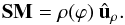 (15)We also suppose that
ρ is a decreasing function of | ϕ | from the axis apex
to any of the legs. More precisely, we suppose that λ is a monotonous
function of ϕ with λ growing from − 90° to
90° as ϕ evolves from − ϕmax to
ϕmax (Fig. 1c). Since
we find no indication of any asymmetry between the legs in the MC data (Sect. 2.4), we suppose
ρ(−ϕ) = ρ(ϕ), and
we present the results only for .
Apart from these general constraints, the flux rope shape is not prescribed, unlike in
Sect. 3, and we deduce it from the observed
distribution
shown in Fig. 5.
(15)We also suppose that
ρ is a decreasing function of | ϕ | from the axis apex
to any of the legs. More precisely, we suppose that λ is a monotonous
function of ϕ with λ growing from − 90° to
90° as ϕ evolves from − ϕmax to
ϕmax (Fig. 1c). Since
we find no indication of any asymmetry between the legs in the MC data (Sect. 2.4), we suppose
ρ(−ϕ) = ρ(ϕ), and
we present the results only for .
Apart from these general constraints, the flux rope shape is not prescribed, unlike in
Sect. 3, and we deduce it from the observed
distribution
shown in Fig. 5.
The conservation of the number of cases implies that the variation in ϕ
is linked to those of λ as in Eq. (10) by 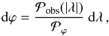 (16)and we suppose that
is uniformly distributed in the interval
[0,ϕmax], so that
(16)and we suppose that
is uniformly distributed in the interval
[0,ϕmax], so that
 .
The integration of Eq. (16) provides
ϕ as a function of λ as
.
The integration of Eq. (16) provides
ϕ as a function of λ as 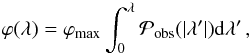 (17)with
λ ≥ 0, ϕ ≥ 0.
(17)with
λ ≥ 0, ϕ ≥ 0.
Next, we relate ρ to λ. Making the derivation of Eq.
(15) with respect to ϕ,
the unit tangent vector at point M is 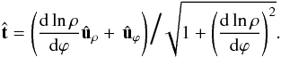 (18)
(18)
The location angle λ is related to
ρ(ϕ) as  (19)
(19)
Using Eq. (16) together with
,
the integration of Eq. (19) implies
 (20)In summary, Eqs.
(17) and (20) provide ϕ and ρ as functions of
λ, so that the axis shape can be derived as a parametric curve in
cylindrical coordinates. It depends on two integration constants
ϕmax and ρmax. The second one is
related to the general scaling of the axis shape, which can be set to 1 AU for the
application to WIND data. However, ϕmax is an intrinsic
freedom parameter of the method, and it is not defined by the in situ observations. We
found in Sect. 3.4 that
ϕmax has a weak effect on the derived
for the forward modeling of the axis with an elliptical shape (Fig. 9). This is consistent with the present results since we have found here
that the observed distribution
is compatible with a wide range of ϕmax values.
(20)In summary, Eqs.
(17) and (20) provide ϕ and ρ as functions of
λ, so that the axis shape can be derived as a parametric curve in
cylindrical coordinates. It depends on two integration constants
ϕmax and ρmax. The second one is
related to the general scaling of the axis shape, which can be set to 1 AU for the
application to WIND data. However, ϕmax is an intrinsic
freedom parameter of the method, and it is not defined by the in situ observations. We
found in Sect. 3.4 that
ϕmax has a weak effect on the derived
for the forward modeling of the axis with an elliptical shape (Fig. 9). This is consistent with the present results since we have found here
that the observed distribution
is compatible with a wide range of ϕmax values.
Finally, we derive Eqs. (17) and (20). Since they involve integrals of the
observed distribution ,
the derived axis shape is expected to be weakly affected by the details of
.
Also, because the integration advances from the apex toward the legs, the growing
uncertainties on
with |λ| are kept for rising values of |λ|; i.e.,
the axis shape is expected to be determined best around the apex and with a growing
uncertainty when going towards the legs.
4.2. Results
The values for the distribution
appearing in Eqs. (17) and (20) can be computed in different ways to
deduce the mean axis shape. First,
can be interpolated by Hermite or spline polynom functions before performing the
integrations. We set  ,
and use the symmetry
,
and use the symmetry  in order to have an interpolation (and not an extrapolation) for all the
λ ranges. First, we find negligible differences between these two types
of interpolation and between different interpolation orders (1 to 3). Second, we use
different numbers of bins to build the
histogram. The number of bins also has a negligible effect on the axis shape, as shown for
10 and 20 bins in Fig. 10a. Finally,
can be fitted by an analytical distribution. The result with a linear function, as shown
in Fig. 5 (black line), provides a very similar axis
shape, as shown in Fig. 10a. Such a result also
holds with other fitting functions such as a Gaussian distribution function. All these
tests confirm that the results derived from Eqs. (17) and (20) are robust, that
is, weakly affected by the local variations in .
in order to have an interpolation (and not an extrapolation) for all the
λ ranges. First, we find negligible differences between these two types
of interpolation and between different interpolation orders (1 to 3). Second, we use
different numbers of bins to build the
histogram. The number of bins also has a negligible effect on the axis shape, as shown for
10 and 20 bins in Fig. 10a. Finally,
can be fitted by an analytical distribution. The result with a linear function, as shown
in Fig. 5 (black line), provides a very similar axis
shape, as shown in Fig. 10a. Such a result also
holds with other fitting functions such as a Gaussian distribution function. All these
tests confirm that the results derived from Eqs. (17) and (20) are robust, that
is, weakly affected by the local variations in .
With the definition of the quality class according to Lepping et al. (1990), we keep only the best and good cases, so qualities 1 and
2. Then,
is more peaked near low |λ| values (Fig. 5b). It implies a slight change in the derived axis shape only far from the apex
(Fig. 10b), while the corresponding
have more differences (Fig. 5). This is again an
effect of the integration present in both Eqs. (17) and (20).
Finally, the main uncertainty on the axis shape is due to the free parameter ϕmax. Indeed its effect is significant, especially away from the apex (Fig. 10c). However, for the expected range of ϕmax, as shown, the results imply that the axis is significantly bent, i.e. more bent than the curvature of a circle of radius ρ(ϕ) = ρ(ϕ = 0). The axis shape is also slightly elongated in the ortho-radial direction (along ûϕ), in agreement with an aspect ratio b/a slightly above 1 when the axis is modeled with an elliptical shape (Sect. 3).
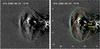 |
Fig. 11 Observational example of a flux rope observed by STEREO-A HI1. The image is derived with running differences. In the right panel, the same image is shown with the front and rear sheaths outlined with green lines. The dashed blue lines are extrapolations towards the Sun. The flux rope axis (red line) is defined at equidistance from the two sheaths. Four twisted structures are marked with orange lines. The coordinate system is the elongation angle in degree from the Sun. This figure is adapted from Möstl et al. (2009). |
5. Comparison with the results of heliospheric imagers
5.1. Description of the analyzed event
The heliospheric imagers on board of STEREO provide a 2D view of the strongest density regions. In the case of CMEs, they typically image the sheath region in front of the CME. The flux rope is best seen as an intensity depletion but its extension, even in projection, is typically difficult to define. Indeed, it can, for example, be partly masked by the sheath and other bright structures present in the background or foreground. The visualization of the flux rope requires the development of sophisticated techniques to remove the huge background present in the heliospheric images (Howard & DeForest 2012, and references therein).
STEREO has so far observed few cases where the flux rope extension can be estimated. To our knowledge, the best case for that purpose is the 2008 June event since the flux rope, observed in situ by STEREO-B, is surrounded by dense plasma, which was imaged by STEREO-A from the side (with a longitude difference of ≈55°). At least two other exceptional cases, with density peaks surrounding the flux rope, have been observed during the two first years of the STEREO mission (Rouillard 2011). However, the 2008 June event remains the most carefully studied among those three.
The associated CME was launched from the Sun on June 1, 2008 at around 21:00 UT and crossed STEREO-B on June 6, 2008 at around 23:00 UT, so about five days later. It is thus a slow CME (Robbrecht et al. 2009; Möstl et al. 2009), and indeed, the in situ plasma measurements found a mean outward velocity of ≈400 km s-1. A clear rotation of the magnetic field is observed at STEREO-B within a low plasma-β region (β ≤ 0.05), but this does not strictly define an MC since its proton temperature is comparable to that of the solar wind with similar speeds (see Fig. 1 of Möstl et al. 2009). Remarkably, the heliospheric imager of STEREO-A detected density structures having a twisted appearance along the whole flux rope (see the orange lines in Fig. 11). From their extensions, these dense structures are expected to be at the periphery of the flux rope.
The flux rope is significantly faster than the front solar wind and a shock is present at the front edge of the sheath. The flux rope is also overtaken by a faster stream detected in situ by both STEREO-B and the imagers of STEREO-A (see Fig. 1 and movies of Möstl et al. 2009). This fast stream creates a reverse shock, and bound from behind the second sheath region that follows the flux rope. Corresponding front and rear sheaths are seen in the heliospheric imagers of STEREO-A as two bright regions bracketing a dim one associated with the flux rope. These imaged sheaths both have two regions of high plasma density as detected in situ by STEREO-B. This association has been clearly established by Möstl et al. (2009) by comparing the timing of the in situ enhanced density regions with those of the bright regions when they overtake STEREO-B. The two external enhanced density regions are expected to come from plasma compression after the plasma crossed the shocks, while the two internal ones could be due to an earlier over expansion of the flux rope. Then, these two peaks of density in each imaged sheath could be the traces of the propagation and expansion sheaths as defined by Siscoe & Odstrcil (2008).
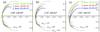 |
Fig. 12 Comparison of the axis shape deduced from in situ measurements of MCs (gray curves) and from the CME observed by STEREO-A HI1 on 2–3 june 2008 (colored curves, the image corresponding to the red curve is shown in Fig. 11). The panels are in the plane of the flux rope axis. We use different geometry to deduce the shape of the axis: a) conic projection on the plane of the sky, b–c) axis plane being inclined on the ecliptic by an angle i and crossing the ecliptic at a longitude Δφ from STEREO-A (see Sect. 5.3). |
5.2. Axis shape estimated with imagers
The relationship found between the in-situ and the imager data implies that the front and rear sheaths bracket the flux rope. In the following, we use this property to estimate the extension of the flux rope from the imagers.
We manually define the central part of both bright regions on Heliospheric Imager (HI) images and suppose that the flux rope axis is at mid-distance (Fig. 11). This procedure has large uncertainties. First, the manual pointing of a bright region has an intrinsic bias. Second, the rear bright region has many structures and is quite difficult to define. Third, the axis may not be exactly at half distance between the two sheaths. Finally, the images are 2D projection of a 3D plasma distribution of unknown shape. We limit the two first uncertainties as much as possible by independently repeating the pointing on different images taken at different times.
We present results obtained only with HI1 since the contrast of the sheaths with the surrounding regions rapidly becomes faint after the entrance in the HI2 field of view (see the movie attached to Möstl et al. 2009). Next, the location of the MC axis at about half distance between the sheaths is locally justified by the in situ measurement of the magnetic field and its force-free reconstruction. The flux rope extension is comparable before and after the closest approach to the axis. Finally, we investigate different geometries to test the projection effect.
The observed bright sheaths are 3D plasma density distribution observed in projection (Fig. 11), and we can deduce their curvature by only adding assumptions. In the line of thinking of Siscoe & Odstrcil (2008), we consider two extremes. One approach is correlated with the hypothesis that the evolution of the sheaths is dominated by the propagation of the ICME. The front one is due to the CME overtaking the slow wind, while the rear sheath can come from the fast wind overtaking the CME. Then, we suppose that the two sheaths are part of spherical shells centered on the Sun. With this simple geometry, the 2D observed shape does not depend on the CME direction, and the observed structure is simply a conic projection on the plane of sky of the dense sheaths (Fig. 12a).
Another approach is to consider the imaged sheaths as a consequence of the flux rope expansion. In such a case, a plasma sheath surrounds the flux rope, and we mostly see the latter when the line of sight is tangent to it. In this second approach, we suppose that the observed sheaths are tracing dense plasma located near the plane of the flux rope. Both, in situ and imager observations, indicate that STEREO-B crossed the flux rope close to its apex. With a plane inclined on the ecliptic by an angle i and with the intersection with the ecliptic at a longitude Δφ from STEREO-A, we project the observations on this plane through a conic projection as viewed from STEREO-A (Fig. 12b,c). In this case an increasing deformation of the flux rope axis is present as the i angle decreases from 90°.
5.3. Comparison of the axis shape derived from in situ and imager data
The estimations of the axis shape from images obtained above are compared with the results of Sect. 4, and in particular with Fig. 10. To do so, we plotted axis shapes for three ϕmax values drawn in the background of Fig. 12. In panel a, it is remarkable that the simple projection on the plane of sky implies a deduced axis very close to the case ϕmax = 30° for the three times shown (this case is the most suitable when considering the upper/lower (northern/southern) branches of the flux rope axis, with only small deviations in the northern shape at the earliest time). We repeated the manual pointing on different images at different observed times. Even shifting the pointing by a half width of the brightenings, the difference between the deduced shapes is less than between the three southern axis deduced at different times in Fig. 12a.
To use the second approach, for which the observed dense plasma is near the flux rope plane, we need to precise the 3D geometry of the event. STEREO-B observed the flux rope in situ and its axis was estimated to cut the ecliptic plane slightly eastward, implying that Δφ ≈ 62° (with Δφ the longitude angle between the flux rope axis and STEREO-A). We find that this angle is different enough from 90° to create a significant deformation of the axis when the inclination i is significantly different from 90°. By fitting the in situ magnetic data with two models, the axis latitude θ was estimated to be 51° and 37° (Möstl et al. 2009). With a crossing close to the flux rope apex, the inclination i has a comparable value. Already the case i = 70° has a marked asymmetry that grows for i = 50° (Fig. 12b,c). It is unlikely that this asymmetry, present in the flux rope plane, would be mostly compensated by a projection deformation to provide the nearly symmetric observed shape, so either the flux rope axis is more orthogonal to the ecliptic plane than inferred from modeling in situ data (implying a rotation of the whole flux rope as it evolves from the Sun toward STEREO-B), either STEREO-A observed more two spherical-like dense shells. All in all, we find that the error on the definition of the brightening shapes on the images is much smaller than the uncertainty coming from the projection of an unknown 3D shape.
The in situ proton density measurements of STEREO-B show comparable width and density for the propagation and expansion sheaths, except from a sharp peak, up to twice denser, for the front expansion sheath (see Fig. 1 Möstl et al. 2009). STEREO-A imagers did not separate the propagation and expansion sheaths both in front and at the rear of the flux rope, so their interpretation as 3D structures is difficult since two different 3D structures are mixed in one bright structure. Here we suppose that the propagation sheath is part of a spherical shell and the expansion sheath has a tube-shaped structure. While the density is comparable in both, the first one has a larger radius of curvature, so a longer quantity of dense plasma is present along the line of sight. Then, it is likely that the propagation sheaths are more contributing to the Thomson scattering of the solar light, so that our most relevant axis shape estimation is shown in Fig. 12a. The main limitation is that both propagation sheaths do not envelope the flux rope closely, so the deduced axis shape could have large biases. Still, the close correspondence found in the axis shape by very different methods is an indication that the systematic bias in each method should not be so large, but they are expected to be close to the differences shown in Fig. 12a.
6. Summary and conclusions
When a spacecraft crosses an MC, detailed in situ measurements of plasma parameters and magnetic field are available only along the spacecraft trajectory. General information on the local cross section of the flux rope is typically derived by solving MHD force-balance equations constrained by the data. Is it possible to realize another step to constrain the whole flux rope? A few multispacecraft observations of the same MC have been realized, but they remain case studies and a large number of spacecraft would be required to sample the flux rope along its axis. Instead, we have information on a large set of MCs crossed once at various locations along their flux ropes. The present study has used this statistical information to derive a mean axis shape. The axis of a particular MC could deviate in respect to this mean shape, but from the method used in the present paper we cannot quantify this deviation.
Our study is based on the results of Lepping & Wu (2010) and their recent extension to 121 MCs observed by WIND spacecraft over 15 years. Each MC was fitted with the Lundquist model. This fit provides an estimation of the local axis direction (its latitude and longitude). This orientation gives implicit information on the location of the spacecraft crossing along the flux rope axis. In order to make this precise, we introduced two new angles to define the local axis direction (Fig. 1): its inclination on the ecliptic (i) and its location angle (λ). If we suppose that the whole axis is planar and loop-shaped as in Figs. 1b,c, then i is the inclination of the axis plane on the ecliptic and, going from one leg to the other, λ evolves continuously from ≈− 90° to ≈90°, with λ = 0 at the apex. Then, i and λ angles are adapted to the geometry of the flux rope.
Could we analyze the results of various MCs altogether? First, we found that the
inclination angle (i) is broadly distributed, and we found no significant
correlation between i and any of the MC parameters. In contrast the
location angle (λ) has a distribution,
 ,
peaked around zero. This distribution is almost symmetric,
,
peaked around zero. This distribution is almost symmetric,
 ,
implying no significant difference between both legs. We then report results derived from
in Fig. 5. We then found no significant dependence of
on the i angle. Furthermore, all correlations of MC parameters with
i angle are very small. We concluded that the MC properties are
independent of the inclination i of the flux rope on the ecliptic.
,
implying no significant difference between both legs. We then report results derived from
in Fig. 5. We then found no significant dependence of
on the i angle. Furthermore, all correlations of MC parameters with
i angle are very small. We concluded that the MC properties are
independent of the inclination i of the flux rope on the ecliptic.
The MCs are launched from various solar longitude and moreover the Sun is rotating, so the
MCs with a low inclination i along the ecliptic are expected to be
uniformly sampled at random positions by WIND spacecraft (located near Earth). Describing
the supposed planar axis with cylindrical coordinates centered on the Sun
(ρ,ϕ) implies that the sampling is expected to be uniform in
ϕ. Then, from the observed
distribution, a flux rope shape can be derived (Sect. 4). Since the
distribution is not significantly dependent of i, the hypothesis of uniform
angular sampling of an MC set is compatible with the study of the distribution for any sets
of MCs considered in this paper (e.g. Fig. 6). MCs
observed with high i values are also broadly sampled along their axis
because MCs are launched from the Sun from a very broad range of latitude that is mostly
maintained as the MCs propagate in interplanetary space (e.g., Ulysses has observed MCs at
latitudes as high as ≈80° in both hemispheres).
We first tested the above idea with a simple global model of the flux rope axis. Supposing
that the axis is part of an ellipse, we found that the distribution of λ is
indeed very sensitive to the axis shape. The observed distribution
is compatible with an aspect ratio of the ellipse around 1.2 with the major axis
perpendicular to the radial from the Sun, but is incompatible with an aspect ratio of unity
(circular shape), as well as an aspect ratio greater than 1.3. In particular, the axis is
not very flat around its apex (i.e. ρ ≈ constant) since it would imply a
distribution
that is much more peaked around λ = 0 than observed.
Next, rather than fitting the above specific model of the axis to
,
we derived a method of computing the mean shape of the axis directly from
.
Since the shape is derived by integration (Eqs. (17) and (20)), the method is
robust to any perturbations of .
Indeed, we verify that very close axis shapes are deduced with various samplings,
interpolations, and fitting functions of
distribution (Fig. 10). Restricting the MC set to the
best observed ones only slightly affects the axis shape away from the apex. Our results are
compatible with previous results of multispacecraft crossings of an MC as summarized in
Figs. 3 and 4 of Burlaga et al. (1990).
One free parameter remains for determining the axis shape from
:
the opening angle between the legs (2 ϕmax, Fig. 7). The forward modeling with an elliptical shape has shown
that the distribution of λ is weakly affected by
ϕmax. However, the negative side is that
ϕmax is not constrained by in situ observations, so that
ϕmax should be provided by another type of observation, such
as heliospheric imagers. The positive side of this is that sets of MCs with different
ϕmax can be combined since they have comparable distributions
of λ. This allows the information of various MCs to be combined to build
without knowing their ϕmax value. This justifies the use of the
full set of WIND MCs, or parts of it, to derive a mean axis shape.
Heliospheric imagers appear at first better suited to constrain the overall shape of MCs. However, they image only the dense sheath present in front of the MCs. In rare cases, a dense sheath is also present at the rear of the MC. Both sheaths bind the flux rope, allowing in principle to define its overall shape; however, the 3D shape of the sheath is unknown, and they partly overlap the flux rope along the line of sight, so that a quantitative estimation of the flux rope shape from imagers also needs a hypothesis on the 3D shape of the sheaths. Moreover, the flux rope axis is not imaged, so its shape can only be determined indirectly from the sheath locations.
We selected a case best suited to defining the axis shape from STEREO-A heliospheric
imagers, while the flux rope was also detected in situ by STEREO-B. Supposing that the
projection only weakly affects the observed shape, we derived an axis shape that is
comparable to the mean axis shape obtained from
and ϕmax ≈ 30°. Since these two derivations of the
axis shape are based on totally different observing techniques, complemented with different
hypotheses, the convergence to a comparable axis shape mutually strengthens their results.
The mean axis shape deduced in this work can be used in several applications. For example, from the axis orientation, locally determined by modeling or by fitting a flux-rope model to the spacecraft magnetic data, the angle λ allows estimating the location of the spacecraft along the mean axis derived in this study. This estimates how far from the apex the spacecraft crossing is in angular distance ϕ (Fig. 7). Another possible application is to determine a minimum field line length by linking the ends of the determined axis shape by straight segments connecting to the Sun. Other field lines of the flux rope are longer because of the twist. This has an application for timing the transport of energetic particles. A third direct application is for space weather, as this flux-rope overall shape can be incorporated in a kinematic model of CME propagation from the Sun (e.g. assuming a self similar evolution).
Finally, the method developed in this work could be applied more broadly. We applied it to
the results of a Lundquist fit of the in situ data, but it can also be applied to any other
method that estimates of the local flux rope orientation, provided enough MCs are analyzed.
Since the deduced axis shape is mainly determined by the slope of
,
which is directly related to the mean of λ, the axis shape estimation does
not need a large number of MCs (e.g. a set of 20 MCs could be sufficient for several
applications which require only an approximate shape). In parallel, it is worth deriving
more constraints on the flux rope shape from imagers, for example, by developing the 3D
forward models of the flux rope and its surrounding sheaths.
Acknowledgments
The work of M.J. is funded by a contract from the AXA Research Fund. This work was partially supported by the Argentinean grants UBACyT 20020090100264 and PIP 11220090100825/10 (CONICET) and by a one- month invitation of S.D. to the Paris Observatory. S.D. is member of the Carrera del Investigador Científico, CONICET. S.D. acknowledges support from the Abdus Salam International Centre for Theoretical Physics (ICTP), as provided in the frame of his regular associateship.
References
- Al-Haddad, N., Roussev, I. I., Möstl, C., et al. 2011, ApJ, 738, L18 [NASA ADS] [CrossRef] [Google Scholar]
- Aulanier, G., Janvier, M., & Schmieder, B. 2012, A&A, 543, A110 [NASA ADS] [CrossRef] [EDP Sciences] [Google Scholar]
- Burlaga, L. F. 1995, Interplanetary magnetohydrodynamics (New York: Oxford University Press) [Google Scholar]
- Burlaga, L., Sittler, E., Mariani, F., & Schwenn, R. 1981, J. Geophys. Res., 86, 6673 [Google Scholar]
- Burlaga, L. F., Lepping, R. P., & Jones, J. A. 1990, Washington DC American Geophysical Union Geophysical Monograph Series, 58, 373 [NASA ADS] [CrossRef] [Google Scholar]
- Canou, A., Amari, T., Bommier, V., et al. 2009, ApJ, 693, L27 [NASA ADS] [CrossRef] [Google Scholar]
- Cheng, X., Zhang, J., Liu, Y., & Ding, M. D. 2011, ApJ, 732, L25 [NASA ADS] [CrossRef] [Google Scholar]
- Cheng, X., Zhang, J., Ding, M. D., Liu, Y., & Poomvises, W. 2013, ApJ, 763, 43 [NASA ADS] [CrossRef] [Google Scholar]
- Cremades, H., & Bothmer, V. 2004, A&A, 422, 307 [NASA ADS] [CrossRef] [EDP Sciences] [Google Scholar]
- Dasso, S. 2009, in IAU Symp. 257, eds. N. Gopalswamy, & D. F. Webb, 379 [Google Scholar]
- Dasso, S., Mandrini, C. H., Démoulin, P., & Farrugia, C. J. 2003, J. Geophys. Res., 108, 1362 [NASA ADS] [CrossRef] [Google Scholar]
- Dasso, S., Mandrini, C. H., Démoulin, P., & Luoni, M. L. 2006, A&A, 455, 349 [NASA ADS] [CrossRef] [EDP Sciences] [Google Scholar]
- Démoulin, P., & Dasso, S. 2009, A&A, 507, 969 [NASA ADS] [CrossRef] [EDP Sciences] [Google Scholar]
- Démoulin, P., Dasso, S., & Janvier, M. 2013, A&A, 550, A3 [NASA ADS] [CrossRef] [EDP Sciences] [Google Scholar]
- Farrugia, C. J., Berdichevsky, D. B., Möstl, C., et al. 2011, J. Atmos. Sol. Terr. Phys., 73, 1254 [NASA ADS] [CrossRef] [Google Scholar]
- Forbes, T. G., Linker, J. A., Chen, J., et al. 2006, Space Sci. Rev., 123, 251 [NASA ADS] [CrossRef] [Google Scholar]
- Goldstein, H. 1983, in Solar Wind Five, NASA CP-2280, ed. M. Neugebauer, 731 [Google Scholar]
- Guo, Y., Schmieder, B., Démoulin, P., et al. 2010, ApJ, 714, 343 [NASA ADS] [CrossRef] [Google Scholar]
- Hidalgo, M. A. 2011, J. Geophys. Res., 116, 2101 [CrossRef] [Google Scholar]
- Howard, T. A. 2011, J. Atmos. Sol. Terr. Phys., 73, 1242 [NASA ADS] [CrossRef] [Google Scholar]
- Howard, T. A., & DeForest, C. E. 2012, ApJ, 746, 64 [Google Scholar]
- Hu, Q., & Sonnerup, B. U. Ö. 2002, J. Geophys. Res., 107, 1142 [CrossRef] [Google Scholar]
- Isavnin, A., Kilpua, E. K. J., & Koskinen, H. E. J. 2011, Sol. Phys., 273, 205 [NASA ADS] [CrossRef] [Google Scholar]
- Kilpua, E. K. J., Jian, L. K., Li, Y., Luhmann, J. G., & Russell, C. T. 2011, J. Atmos. Sol. Terr. Phys., 73, 1228 [Google Scholar]
- Kleimann, J. 2012, Sol. Phys., 281, 353 [NASA ADS] [Google Scholar]
- Krall, J. 2007, ApJ, 657, 559 [NASA ADS] [CrossRef] [Google Scholar]
- Larson, D. E., Lin, R. P., McTiernan, J. M., et al. 1997, Geophys. Res. Lett., 24, 1911 [NASA ADS] [CrossRef] [Google Scholar]
- Leitner, M., Farrugia, C. J., Möstl, C., et al. 2007, J. Geophys. Res., 112, A06113 [NASA ADS] [CrossRef] [Google Scholar]
- Lepping, R. P., & Wu, C. C. 2010, Ann. Geophys., 28, 1539 [NASA ADS] [CrossRef] [Google Scholar]
- Lepping, R. P., Burlaga, L. F., & Jones, J. A. 1990, J. Geophys. Res., 95, 11957 [NASA ADS] [CrossRef] [Google Scholar]
- Lepping, R. P., Wu, C.-C., & Berdichevsky, D. B., 2005, Ann. Geophys., 23, 2687 [NASA ADS] [CrossRef] [Google Scholar]
- Lugaz, N., & Roussev, I. 2011, J. Atmos. Sol. Terr. Phys., 73, 1187 [NASA ADS] [CrossRef] [Google Scholar]
- Lundquist, S. 1950, Ark. Fys., 2, 361 [Google Scholar]
- Marubashi, K. 1997, in Coronal Mass Ejections, Geophysical Monograph 99, 147 [Google Scholar]
- Marubashi, K., & Lepping, R. P. 2007, Ann. Geophys., 25, 2453 [NASA ADS] [CrossRef] [Google Scholar]
- Marubashi, K., Cho, K.-S., Kim, Y.-H., Park, Y.-D., & Park, S.-H. 2012, J. Geophys. Res., 117, 1101 [Google Scholar]
- Masson, S., Démoulin, P., Dasso, S., & Klein, K.-L. 2012, A&A, 538, A32 [NASA ADS] [CrossRef] [EDP Sciences] [Google Scholar]
- Möstl, C., Farrugia, C. J., Temmer, M., et al. 2009, ApJ, 705, L180 [NASA ADS] [CrossRef] [Google Scholar]
- Mulligan, T., & Russell, C. T. 2001, J. Geophys. Res., 106, 10581 [NASA ADS] [CrossRef] [Google Scholar]
- Mulligan, T., Russell, C. T., Anderson, B. J., et al. 1999, in Solar Wind Nine, eds. S. R. Habbal, R. Esser, J. V. Hollweg, P. A. Isenberg, AIP Conf. Proc., 471, 689 [Google Scholar]
- Nakagawa, T., & Matsuoka, A. 2010, J. Geophys. Res. (Space Physics), 115, 10113 [NASA ADS] [CrossRef] [Google Scholar]
- Nakwacki, M., Dasso, S., Démoulin, P., Mandrini, C. H., & Gulisano, A. M. 2011, A&A, 535, A52 [NASA ADS] [CrossRef] [EDP Sciences] [Google Scholar]
- Owens, M. J., Démoulin, P., Savani, N. P., Lavraud, B., & Ruffenach, A. 2012, Sol. Phys., 278, 435 [NASA ADS] [CrossRef] [Google Scholar]
- Patsourakos, S., Vourlidas, A., & Stenborg, G. 2013, ApJ, 764, 125 [NASA ADS] [CrossRef] [Google Scholar]
- Pick, M., Forbes, T. G., Mann, G., et al. 2006, Space Sci. Rev., 123, 341 [NASA ADS] [CrossRef] [Google Scholar]
- Reisenfeld, D. B., Gosling, J. T., Forsyth, R. J., Riley, P., & St. Cyr, O. C. 2003, Geophys. Res. Lett., 30, 8031 [NASA ADS] [CrossRef] [Google Scholar]
- Robbrecht, E., Patsourakos, S., & Vourlidas, A. 2009, ApJ, 701, 283 [Google Scholar]
- Romashets, E., & Vandas, M. 2009, A&A, 499, 17 [NASA ADS] [CrossRef] [EDP Sciences] [Google Scholar]
- Romashets, E. P., & Vandas, M. 2003, Geophys. Res. Lett., 30, 2065 [Google Scholar]
- Rouillard, A. P. 2011, J. Atmos. Sol. Terr. Phys., 73, 1201 [Google Scholar]
- Ruffenach, A., Lavraud, B., Owens, M. J., et al. 2012, J. Geophys. Res., 117, A09101 [NASA ADS] [CrossRef] [Google Scholar]
- Schmieder, B., Demoulin, P., & Aulanier, G. 2013, Adv. Space Res., 51, 1967 [NASA ADS] [CrossRef] [Google Scholar]
- Siscoe, G., & Odstrcil, D. 2008, J. Geophys. Res., 113, A00B07 [CrossRef] [Google Scholar]
- Sonnerup, B. U. Ö., Hasegawa, H., Teh, W.-L., & Hau, L.-N. 2006, J. Geophys. Res., 111, 9204 [CrossRef] [Google Scholar]
- Thernisien, A. 2011, ApJS, 194, 33 [Google Scholar]
- Thernisien, A. F. R., Howard, R. A., & Vourlidas, A. 2006, ApJ, 652, 763 [Google Scholar]
- Thernisien, A., Vourlidas, A., & Howard, R. A. 2011, J. Atmosph. Sol.-Terrest. Phys., 73, 1156 [Google Scholar]
- Vandas, M., & Romashets, E. P. 2003, A&A, 398, 801 [NASA ADS] [CrossRef] [EDP Sciences] [Google Scholar]
- Vandas, M., Odstrčil, D., & Watari, S. 2002, J. Geophys. Res., 107, 1236 [Google Scholar]
- Wimmer-Schweingruber, R. F., Crooker, N. U., Balogh, A., et al. 2006, Space Sci. Rev., 123, 177 [NASA ADS] [CrossRef] [Google Scholar]
- Wood, B. E., Howard, R. A., Thernisien, A., Plunkett, S. P., & Socker, D. G. 2009, Sol. Phys., 259, 163 [NASA ADS] [CrossRef] [Google Scholar]
- Wood, B. E., Wu, C.-C., Howard, R. A., Socker, D. G., & Rouillard, A. P. 2011, ApJ, 729, 70 [Google Scholar]
- Xie, H., Gopalswamy, N., & St. Cyr, O. C. 2013, Sol. Phys., 284, 47 [NASA ADS] [CrossRef] [Google Scholar]
All Figures
|
Fig. 1 Definitions of the angles and flux-rope geometry. a) Schema defining the
angles of the local MC axis direction. It is a local view of panel b).
The unit vector |
| In the text | |
|
Fig. 2 Properties of MCs observed at 1 AU versus the location angle (λ in degree). The correlations are shown for the mean MC velocity (V in km s-1), the MC radius (R in AU), the axial magnetic field strength (B0 in nT), and the axis inclination (i in degree) for the full set of MCs. λ > 0 and λ < 0 are shown in red and blue, respectively, and the abscissa, |λ|, allows comparing the two leg sides of the flux rope (Fig. 1c). The straight lines are linear fits to the data points (MCs) showing the tendency. The results with the total MC set are shown in black (linear fit and top labels). cP and cS are the Pearson and Spearman rank correlation coefficients, respectively, and “fit” is the least-square fit of a straight line (in black) to the full data set. |
| In the text | |
|
Fig. 3 Properties of MCs observed at 1 AU versus the axis inclination on the ecliptic (i in degree). The correlations are shown for the mean MC velocity (V in km s-1), the MC radius (R in AU), the axial magnetic field strength (B0 in nT), and the asymmetry factor (asf in %) for the full set of MCs. The asymmetry factor (asf, see Lepping et al. 2005) measures twice the time difference between the middle of the MC time interval and the closest approach (“center time”). It is expressed in % of the MC event duration. It has been introduced to measure how far in time the peak in the modeled magnetic field is from the midpoint of observed MC. The drawing convention is the same as in Fig. 2. |
| In the text | |
|
Fig. 4 Probability distribution, |
| In the text | |
|
Fig. 5 Probability distribution, |
| In the text | |
|
Fig. 6 Property of the probability distribution |
| In the text | |
|
Fig. 7 Diagram defining a model of the flux rope axis with an elliptical shape. The legs are represented by straight and radial segments tangent to the ellipse and linking it to the Sun. ϕ is the angle of the cylindrical coordinates (ρ,ϕ). The point C is the ellipse center and M is the point of interest (where the spacecraft crosses the flux rope). |
| In the text | |
|
Fig. 8 Probability distribution of the location angle λ (left
panels) and the corresponding axis shape (right panels)
for the elliptical model of the flux rope axis (defined in Fig. 7). Since the model is symmetric,
|
| In the text | |
|
Fig. 9 Comparison of the probability distribution of the location angle λ for the elliptical model of the flux rope axis with a given aspect ratio b/a in each panel (see Fig. 7). The distributions are normalized as in Fig. 8 and the dotted curve is the distribution for a small circular front. The maximum extension angle ϕmax only has a weak effect on the distribution shape compared to the strong effect of the aspect ratio b/a. |
| In the text | |
|
Fig. 10 Mean flux-rope axis deduced from the probability distribution
|
| In the text | |
|
Fig. 11 Observational example of a flux rope observed by STEREO-A HI1. The image is derived with running differences. In the right panel, the same image is shown with the front and rear sheaths outlined with green lines. The dashed blue lines are extrapolations towards the Sun. The flux rope axis (red line) is defined at equidistance from the two sheaths. Four twisted structures are marked with orange lines. The coordinate system is the elongation angle in degree from the Sun. This figure is adapted from Möstl et al. (2009). |
| In the text | |
|
Fig. 12 Comparison of the axis shape deduced from in situ measurements of MCs (gray curves) and from the CME observed by STEREO-A HI1 on 2–3 june 2008 (colored curves, the image corresponding to the red curve is shown in Fig. 11). The panels are in the plane of the flux rope axis. We use different geometry to deduce the shape of the axis: a) conic projection on the plane of the sky, b–c) axis plane being inclined on the ecliptic by an angle i and crossing the ecliptic at a longitude Δφ from STEREO-A (see Sect. 5.3). |
| In the text | |
Current usage metrics show cumulative count of Article Views (full-text article views including HTML views, PDF and ePub downloads, according to the available data) and Abstracts Views on Vision4Press platform.
Data correspond to usage on the plateform after 2015. The current usage metrics is available 48-96 hours after online publication and is updated daily on week days.
Initial download of the metrics may take a while.