| Issue |
A&A
Volume 556, August 2013
|
|
|---|---|---|
| Article Number | A127 | |
| Number of page(s) | 10 | |
| Section | The Sun | |
| DOI | https://doi.org/10.1051/0004-6361/201220848 | |
| Published online | 08 August 2013 | |
Can spicules be detected at disc centre in broad-band Ca ii H filter imaging data?⋆
1 Instituto de Astrofísica de Canarias (IAC), C/ Via Lactéa, 38205 La Laguna (Tenerife), Spain
e-mail: This email address is being protected from spambots. You need JavaScript enabled to view it.
2 Departamento de Astrofísica, Universidad de La Laguna, 38206 La Laguna (Tenerife), Spain
3 National Solar Observatory (NSO), Sunspot, NM 88349, USA
4 Kiepenheuer-Institut für Sonnenphysik (KIS), Schöneckstr. 6, 79104 Freiburg, Germany
e-mail: This email address is being protected from spambots. You need JavaScript enabled to view it.
5 Leibniz-Institut für Astrophysik Potsdam (AIP), An der Sternwarte 16, 14482 Potsdam, Germany
e-mail: This email address is being protected from spambots. You need JavaScript enabled to view it.
Received: 4 December 2012
Accepted: 21 June 2013
Abstract
Context. Recently, a possible identification of type II spicules in broad-band (full-width at half-maximum (FWHM) of ~0.3 nm) filter imaging data in Ca ii H on the solar disc was reported.
Aims. We estimate the formation height range contributing to broad-band and narrow-band filter imaging data in Ca ii H to investigate whether spicules can be detected in such observations at the centre of the solar disc.
Methods. We applied spectral filters of FWHMs from 0.03 nm to 1 nm to observed Ca ii H line profiles to simulate Ca imaging data. We used observations across the limb to estimate the relative intensity contributions of off-limb and on-disc structures. We compared the synthetic Ca filter imaging data with intensity maps of Ca spectra at different wavelengths and temperature maps at different optical depths obtained by an inversion of these spectra. In addition, we determined the intensity response function for the wavelengths covered by the filters of different FWHM.
Results. In broad-band (FWHM = 0.3 nm) Ca imaging data, the intensity emitted off the solar limb is about 5% of the intensity at disc centre. For a 0.3-nm-wide filter centred at the Ca ii H line core, up to about one third of the off-limb intensity comes from emission in Hϵ. On the disc, only about 10 to 15% of the intensity transmitted through a broad-band filter comes from the line-core region between the H1 minima (396.824 to 396.874 nm). No traces of elongated fibrillar structures are visible in the synthetic Ca broad-band imaging data at disc centre, in contrast to the line-core images of the Ca spectra. The intensity-weighted response function for a 0.3-nm-wide filter centred at the Ca ii H line core peaks at about log τ ~ −2 (z ~ 200 km). Relative contributions from atmospheric layers above 800 km are about 10%. The inversion results suggest that the slightly enhanced emission around the photospheric magnetic network in broad-band Ca imaging data is caused by a thermal canopy at a height of about 600 km.
Conclusions. Broad-band (~0.3 nm) Ca ii H imaging data do not trace upper chromospheric structures such as spicules in observations at the solar disc because of the too small relative contribution of the line core to the total wavelength-integrated filter intensity. The faint haze around network elements in broad-band Ca imaging observations at disc centre presumably traces thermal canopies in the vicinity of magnetic flux concentrations instead.
Key words: Sun: chromosphere / Sun: photosphere / techniques: spectroscopic
Appendix A is available in electronic form at http://www.aanda.org
© ESO, 2013
1. Introduction
One of the most successful recent broad-band (~0.3 nm) filter-imaging systems in use in solar physics is the imaging channel in the chromospheric Ca ii H line on-board the Hinode satellite (Kosugi et al. 2007; Tsuneta et al. 2008). The seeing-free data from the Hinode mission are an unique source of high-quality solar observations at a constant spatial resolution. One topic that was revived by the advent of the Hinode Ca imaging data were solar spicules that are seen in chromospheric lines at and beyond the solar limb (Beckers 1968; Sterling 2000). The Hinode Ca imaging data triggered a whole series of investigations because for the first time the temporal evolution of individual spicules could be followed in detail (cf. de Pontieu et al. 2007; Sterling et al. 2010).
On-disc counterparts of spicules were identified in observed line spectra by their velocity signature, i.e. rapid Doppler excursions of chromospheric lines towards the blue that imply fast upward motion (Langangen et al.2008; Rouppe van der Voort et al.2009; Sekse et al.2012; but see also Judge et al.2011). Recently, de Wijn (2012; DW12) interpreted a faint intensity haze around the photospheric magnetic network in a difference image of Hinode Ca imaging data and simultaneous line-core intensity maps of the photospheric Fe i line at 630.15 nm as the signature of type II spicules. He argued that the Hinode Ca filter has some significant chromospheric contribution that would produce this haze as a consequence of chromospheric features. While this argument holds for Lyot-type filters (e.g. Öhman 1938; Lyot 1944; Wang et al. 1995; Skomorovsky et al. 2012) that can have spectral pass-bands down to 0.01 nm (e.g. Reardon et al.2009; RE09), it is not immediately clear whether the same is true for broad-band interference filters with 0.1 to 1 nm full-width at half-maximum (FWHM) band passes.
The investigation of the intensity response of the Ca ii H broad-band filter of Hinode by Carlsson et al. (2007) yielded a maximal response at a height of about 250 km, whereas Jafarzadeh et al. (2013) reported about 450 km for the 0.18 nm filter of SuFi on-board of the Sunrise balloon mission (Barthol et al. 2011). Pietarila et al. (2009) found that 90% of the intensity in a 0.15-nm-wide Ca filter should originate from layers below 500 km. RE09 found “no significant chromospheric signature in the Hinode/SOT Ca II H quiet-Sun filtergrams” from a comparison with Ca ii IR spectra. An identification of type II spicules in broad-band Ca imaging data at disc centre is thus rather surprising, but we note that the results above referred to the quiet Sun with low magnetic activity.
Outside the solar limb even broad-band Ca filter imaging data trace without doubt chromospheric structures because of the absence of any photospheric radiation, but it is not clear if the same applies to observations on the solar disc. Here, we investigate the contribution of off-limb features such as spicules to the wavelength-integrated intensity for the case of broad-band filter observations on the solar disc by comparing the latter with resolved Ca ii H spectra and synthetic imaging data obtained by a multiplication of the spectra with filter curves of different FWHM.
Section 2 describes the various data sets used. The observational results of the Ca ii H spectroscopy and the (synthetic) imaging data at the centre of the solar disc and at the solar limb are presented in Sect. 3, together with the calculation of theoretical intensity response functions. The results are discussed in Sect. 4, while Sect. 5 provides our conclusions. Appendix A investigates the relative contribution of the chromospheric Hϵ line at 397 nm to the Hinode Ca broad-band prefilter.
2. Observations and creation of synthetic Ca images
The primary data used in this study are two observations of Ca ii H spectra obtained with the POlarimetric LIttrow Spectrograph (POLIS; Beck et al. 2005). One data set contains Ca spectra at and beyond the solar limb, and is described in detail in Beck & Rezaei (2011a) and Beck et al. (2011). These data are also available on-line (Beck & Rezaei 2011b). The second POLIS data set was taken at the centre of the solar disc and is described in detail in Beck et al. (2009, BE09; 2012). Figures 2 and 5 below show overview maps of these observations. Because the spectral range provided by the default POLIS Ca CCD (cf. Fig. 1) does not cover the FWHM of 1 nm required for the broadest Ca filter under investigation, we used a data set recorded at disc centre on 29 June 2010 with a PCO 4000 as Ca camera inside of POLIS instead (cf. the setup described in Beck & Rezaei 2012).
For the comparison to the results derived from the spectra, we used images in Ca ii K taken with a Lyot filter of a FWHM of 0.03 nm. This Lyot filter is part of the slit-jaw (SJ) camera system (Kentischer 1995) at the German Vacuum Tower Telescope (VTT; Schröter et al. 1985). For the disc-centre observations taken on 21 August 2006, the Lyot filter was mounted in front of the Triple Etalon SOlar Spectrometer (TESOS; Kentischer et al. 1998; Tritschler et al. 2002) as part of an imaging setup (cf. Beck et al. 2007), while near the limb (24 April 2011), a PCO 4000 was mounted as SJ camera instead of the default video camera (see Martínez González et al.2012 for the science data of this observation). We also used two Ca ii H images at similar locations from the Hinode Solar Optical Telescope (Kosugi et al. 2007; Tsuneta et al. 2008). They were taken on 27 August 2011 and on 19 February 2007 near disc centre and at the limb, respectively. A third Ca image at disc centre was recorded with a 1-nm-wide prefilter that was mounted in an additional imaging channel in front of the Göttingen Fabry-Perot Interferometer (GFPI; Puschmann et al. 2006; Bello González & Kneer 2008) for complementary ground-based observations during the SUNRISE flight in 2009. The Ca ii H imaging data used here were observed on 07 June 2009 in combination with G-band imaging and spectropolarimetric measurements with the GFPI in the Fe i line at 630.25 nm. Details on these data and the applied image reconstruction techniques, as for example the (multi-object) multi-frame blind deconvolution ([MO]MFBD; van Noort et al. 2005) and speckle reconstruction (Puschmann & Sailer 2006), can be found in Puschmann & Beck (2011).
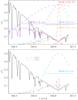 |
Fig. 1 Average observed and theoretical Ca profiles with different filters. Top panel: average observed Ca profile at disc centre (black line). Purple/blue/orange/red dashed lines: Gaussians with FWHM of 1 nm, 0.3 nm, 0.22 nm, and 0.03 nm, respectively, centred at 396.85 nm. Purple/blue/orange/red solid lines: multiplication of the observed profile with the filter transmission. Bottom panel: multiplication of NLTE FALC/FALF profiles (blue-dash-triple-dotted/red-dash-dotted lines) with a 0.3 nm filter. |
To simulate the Hinode Ca imaging data, we multiplied all spectrally resolved observed line profiles with Gaussians of FWHM = 0.22 nm (Carlsson et al. 2007) and 0.3 nm (Tsuneta et al. 2008), respectively (cf. Fig. 1, called broad-band imaging in the following). For the simulation of images taken with a Lyot-type filter, we multiplied the spectra observed with the default POLIS Ca CCD with a transmission profile of FWHM = 0.03 nm (called narrow-band imaging in the following). Finally, for the comparison with the filter images of FWHM = 1 nm, we multiplied the Ca spectra observed with the PCO 4000 camera inside of POLIS with the transmission profile of the corresponding filter.
Applying the respective filters to the average spectrum observed at disc centre (top panel of Fig. 1) reveals that for the narrow-band filter, only wavelengths at and near the line core are sampled, with the maximum of the transmitted intensity at the line core. In contrast, the maximum of the transmitted intensity is found far away from the line core or even the H1 intensity minima for all broad-band filters. The spectral wavelength range in which the transmitted intensity in the line wing is higher than in the line core is also significantly wider than the line-core region itself for broad-band imaging. In the following, the synthetic broad-band data corresponding to the filter with a FWHM of 0.3 nm will be used as being representative for the Hinode Ca imaging data, because the differences between the two broad-band filters of 0.22 nm and 0.3 nm FWHM are minor (cf. Fig. 10 below).
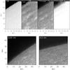 |
Fig. 2 Overview of the observations at the solar limb. Top panel, left to right: 2D maps obtained from the spectra in the outer wing (OW), the line core (Icore, linear display), the synthetic Ca broad-band imaging data (linear display), and the same in logarithmic and clipped display. Bottom panel, left to right: contrast-enhanced Ca ii K Lyot-filter and Hinode Ca ii H broad-band filter images at the solar limb. |
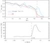 |
Fig. 3 Intensity and relative core contribution on radial cuts normalized to the intensity at disc centre. Top panel: average intensity in OW (red line), Ca line core Icore (blue line) and synthetic Ca broad-band imaging data (black line). Bottom panel: relative contribution of the line core to the broad-band filter intensity. The dashed vertical lines denote the location of the limb. |
As additional reference apart from the observed spectra we used Ca ii H profiles synthesized from the solar atmospheric models FALC and FALF (Fontenla et al. 2006) in non-local thermal equilibrium (NLTE) with the RH code (Uitenbroek 2000). Beck et al. (2013b) discussed the match of such NLTE profiles with individual and average observed Ca spectra. These synthetic NLTE profiles were only multiplied with the transmission profile of the 0.3 nm filter (lower panel of Fig. 1). For both synthetic profiles, the maximum of the transmitted intensity is located near the Ca line core, but the spectral extent of the emission peaks is smaller than the wavelength range in the line wing that shows a transmitted intensity of comparable amplitude. To estimate the relative contributions of line wing and line core to the total intensity transmitted by the Hinode broad-band filter, we integrated the transmitted intensity from the outer wing up to 396.824 nm (H1V) for the former, and from 396.824 to 396.874 nm for the latter. For the contribution from the red wing, which is not covered in the standard POLIS spectra, we assumed the same contribution as for the blue wing. On the disc, the contribution of Hϵ at 397 nm to the total intensity is negligible (cf. Appendix A). The relative contribution of the Ca line core to the total intensity transmitted through the filter is about 10% for the FAL profiles.
3. Results
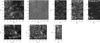 |
Fig. 4 Disc centre observations with different filter widths. Top row, left to right: Ca ii K Lyot image (0.03 nm), Hinode/FG broad-band Ca ii H image (0.3 nm), MFBD-reconstructed Ca image (1 nm), co-spatial MOMFBD line-core image of Fe i at 630.25 nm and the unsigned wavelength-integrated Stokes V signal of this line recorded with the GFPI. Bottom row, left to right: synthetic images derived by applying the corresponding filters of the top row to Ca spectra observed at disc centre. The synthetic image for the 1-nm-wide filter was obtained from the Ca spectra taken with a PCO camera inside of POLIS at a different time. All images are scaled individually inside their full dynamical range. |
3.1. Limb observations
For the limb observations, the intensity in the outer wing (OW, at about 396.397 nm; cf. Rezaei et al. 2007; Beck et al. 2008) of the Ca line and the line-core intensity Icore of Ca ii H (fixed wavelength at 396.85 nm) are shown in the top panel of Fig. 2, together with the synthetic Hinode broad-band Ca imaging data. The latter map is shown twice with different display ranges (linear and logarithmic with clipping). Unlike in the Ca line-core image, the off-limb structures in the synthetic Ca imaging data cannot be seen in the linear display mode because of the strong intensity decrease beyond the limb (compare with Fig. 4 of DW12). The off-limb intensity in the line-core image is rather uniform with a minor variation along the limb.
The lower two panels of Fig. 2 show a Ca ii K image near the limb taken with the 0.03-nm-wide Lyot filter and a broad-band Ca ii H image from Hinode for comparison. Both images were treated with an un-sharp masking to remove the radial intensity gradient and to enhance small-scale structures. Both filter images and the synthetic Ca broad-band image show a characteristic grainy structure of about 1 Mm extent that is absent from the Ca ii H line-core image. Note that the Ca line-core image has exactly the same spatial resolution as the synthetic Ca broad-band image, therefore, the observed differences between the two images are real and cannot be caused by any spatial resolution effects.
The upper panel of Fig. 3 shows the average intensity in the OW, the Ca line core and the synthetic Ca broad-band imaging data on radial cuts perpendicular to the limb. In the OW, the intensity drops to zero beyond the limb, while Icore shows a local intensity maximum at about 2 Mm height above the limb. The limb location was determined visually in the OW map. The intensity of the synthetic Ca broad-band image (black line) decreases monotonically from about 10% of disc-centre intensity right at the limb to 2% at a height of 7 Mm above the limb. Thus, the residual intensity in the synthetic Ca broad-band imaging data is only about 5% of the intensity at disc centre for the height range that can be attributed to off-limb spicules.
The lower panel of Fig. 3 shows that off the limb the line-core region (396.824 to 396.874 nm) contributes dominantly to the total synthetic Hinode broad-band filter intensity. The line-core contribution to the filter reaches only a maximum of about 50% because the Ca line width off the limb exceeds the 50 pm range attributed to the Ca line core here (cf. Fig. 5 of Beck & Rezaei 2011a). However, the relative contribution of the line core drops rapidly near the limb and remains at about 10% on the disc.
3.2. Disc centre observations
Figure 4 compares a set of Ca images taken with different filter widths (0.03 nm, 0.3 nm and 1 nm) at disc centre. The spatial structuring changes significantly from one image to the next. The Lyot-filter image shows spatially extended areas of low intensity of up to 10′′ diameter (cf. Rezaei et al. 2008), and an enhanced intensity around the network. Granular structure is absent. The Hinode Ca image is spatially much more uniform and exhibits an inverse granulation pattern on which a few isolated small-scale brightenings are overlayed. The image taken with the broadest of the Ca filters (1 nm) shows similar isolated small-scale brightenings, but the global pattern has changed from inverse to regular granulation instead. A comparison of the latter image with the simultaneous, co-spatial line-core image and the unsigned wavelength-integrated Stokes V signal, ∫ | V(λ) | dλ, of the Fe i line at 630.25 nm line (denoted by Stokes | V | in the following) extracted from the GFPI spectra (rightmost two panels in the top row of Fig. 4) reveals the strong imprint of photospheric magnetic fields on both the line-core intensity image (cf. Puschmann et al. 2007) and the Ca imaging data for a filter with a FWHM of 1 nm, while the Fe i line-core image shows a background pattern of inverse granulation again. The bright features in the 1-nm Ca filter image are significantly smaller than in the line-core image of the photospheric line and show no intensity enhancements in their surroundings, while both images have a similar spatial resolution (Puschmann & Beck 2011).
The maps in the lower row show the corresponding images obtained by applying the respective filters of the upper row to observed Ca spectra. The change of the background pattern from the absence of granulation through inverse granulation towards regular granulation is well reproduced by the synthetic images. The synthetic Lyot-type and 0.3 nm-filter images were obtained from the same set of spectra and therefore have exactly the same spatial resolution. The extent of the enhanced intensity (haze) at and around the magnetic photospheric network (cf. with the Stokes | V | map in Fig. 5) reduces significantly for the 0.3-nm-wide filter and is absent from the 1-nm-filter images.
Figure 5 shows maps of line parameters derived from the Ca spectra observed with POLIS at disc centre, the synthetic broad-band image, Stokes | V | and the line-core intensity of the Fe i line at 630.25 nm observed with the second channel of POLIS, and the difference image of the synthetic Ca broad-band and the Fe i line-core map (compare with DW12, his Fig. 1, and RE09, their Fig. 7). For the difference image, the relative intensities of the Fe line-core map in the full field of view (FOV) were re-scaled by a linear regression to the intensity range of the synthetic Ca broad-band imaging data. The difference image highlights regions with a relative intensity excess in the broad-band Ca imaging data over the Fe line-core map. To visualize the haze around the network, we laid cuts through the Fe line-core map, the synthetic Ca broad-band image and the Ca line-core map (Fig. 6) after balancing their dynamical range in the same way by linear regression. The haze is visible as a weak intensity enhancement of the synthetic Ca broad-band image over the Fe line-core intensity. The Ca line-core image usually exceeds both of the other quantities over an even larger area.
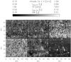 |
Fig. 5 Overview maps of the POLIS observation at disc centre. Bottom row, left to right: OW, Icore of Ca ii H and Stokes | V | signal of the Fe i line 630.25 nm. Top row, left to right: Icore of Fe i at 630.25 nm, synthetic Ca broad-band imaging data and difference image of the latter two. The dotted white lines denote the locations of the cuts shown in Fig. 6. |
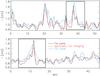 |
Fig. 6 Cuts along the dotted white lines in Fig. 5 through the Fe line-core map (black lines), the synthetic Ca broad-band imaging (red lines) and the Ca line-core intensity map (blue lines). All intensities have been re-scaled to the same dynamical range by linear regression. The black rectangles mark locations of network and their surroundings. |
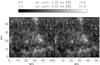 |
Fig. 7 Relative contribution of the line core to the filter intensity at the disc centre. Left/right panel: for filters of FWHM = 0.22 and 0.3 nm, respectively. |
The synthetic Ca imaging data match the line-core intensity of the photospheric Fe i line well, as noted by DW12, but the Ca line-core image shows quite a different pattern. Starting from the locations of the photospheric magnetic flux as outlined in the map of Stokes | V |, elongated slender brightenings of several Mm length can be seen in the Ca line-core intensity (fibrils; Zirin 1974; Marsh 1976; Pietarila et al. 2009; de la Cruz Rodríguez & Socas-Navarro 2011) that also have a counterpart in the line-of-sight (LOS) velocities of the Ca line core (cf. BE09, their Fig. 5).
Comparing the true Ca line-core image (middle bottom panel in Fig. 5, FWHM = 0.0038 nm1) even with a (synthetic) Lyot-type filter image (left column in Fig. 4, FWHM 0.03 nm) shows that the extent of the enhanced intensity around network fields is significantly larger, and consequently, the size of regions with reduced intensity is significantly smaller in the Ca line-core image. The difference image of the synthetic broad-band Ca imaging data and the Fe line-core map shows no traces of fibrils, unlike the Ca line-core image and the LOS velocity map. The comparison of the Ca line-core image with the Stokes | V | signal reveals which of the Ca brightenings are not related to magnetic fields, e.g. the prominent bright grain (cf. Rutten & Uitenbroek 1991; Carlsson & Stein 1997; Beck et al. 2013b) at x,y ~ 50 Mm, 35 Mm. Such features are usually absent in the synthetic broad-band imaging data (top middle panel of Fig. 5), but appear in the synthetic Lyot-filter image (lower-left panel of Fig. 4).
For the average quiet-Sun profile observed at disc centre, about 9% (FALC: 10%, FALF: 13%) of the total intensity transmitted by the broad-band filter comes from the line-core region (396.824 to 396.874 nm). The relative contribution of the line-core region to the filter intensity varies between 4 and 15% across the observed FOV at disc centre (Fig. 7), with an average contribution of 8 ± 1%. For the synthetic filter with 0.22 nm FWHM, the corresponding numbers are between 7 and 21%, with a mean value of 13 ± 1%. The highest values are attained in the centre of the magnetic network (compare Fig. 7 with the Stokes | V | map in Fig. 5), while the lowest values correspond to reversal-free profiles (cf. Rezaei et al. 2008). The enhanced relative contribution of the line core to the total filter intensity on locations of photospheric magnetic fields does, however, not instantly imply a stronger chromospheric contribution to the broad-band filter imaging in the network. On locations of photospheric magnetic fields, the intensity of the Ca line core is raised at all wavelengths, i.e. also outside of the emission core, by a contribution from an atmosphere with a locally increased temperature, but not necessarily a chromospheric temperature rise (e.g. Fig. 17 of Beck et al. 2008).
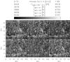 |
Fig. 8 Temperature maps at disc centre. Bottom row, left to right: at optical depths of log τ = −0.6, − 1.6, and − 3.6. Top row, left to right: at log τ = −5.1, and averaged over − 0.6 to − 5.1. The top rightmost panel shows the synthetic Ca broad-band image. The white dashed lines in the temperature map at log τ = −5.1 denote the locations of the spatial cuts shown in Fig. 11. |
Figure 8 shows temperature maps at different atmospheric layers from the photosphere to the lower chromosphere. The temperature was obtained on an optical depth scale related to τ500 nm by applying the inversion approach of Beck et al. (2013a) to the observed Ca spectra that assumes local thermal equilibrium (LTE). Comparing the synthetic Ca imaging data with the temperature maps reveals a close match of the former to the temperature at log τ = −1.6, and an acceptable match to the temperature averaged between log τ = −0.6 and −5.1, but similar to the Ca line-core intensity, the temperature map at log τ = −5.1 shows a different structuring than the synthetic Ca broad-band imaging data. Non-LTE effects should become important in the layers above z ~ 400 km (log τ ~ −3.2; e.g. Rammacher & Ulmschneider 1992), with the main effect of a decoupling between kinetic temperature and emergent intensity. If included in an inversion, NLTE effects would presumably increase the spatial temperature variations relative to the LTE case and therefore additionally reduce the similarity between the temperature maps above log τ ~ − 3.2 and the synthetic Ca imaging data. The visual comparison thus suggests that the intensity in the synthetic Ca imaging data originates from below the formation height of the line core, or log τ = −5.1, respectively, and pertains to a region that shows no clear signature of fibrils in either intensity or velocity maps.
To obtain a quantitative measure of the formation heights that contribute to the synthetic Ca broad-band imaging data, we calculated the intensity response function (cf. Cabrera Solana et al. 2005) R of wavelengths in the Ca ii H line in LTE (lower panel of Fig. 9; see also Carlsson et al. 2007; Pietarila et al. 2009; Jafarzadeh et al. 2013). The values at each wavelength λ were separately normalized to the maximum response R(λ), therefore the response function holds individually for each wavelength. The filter imaging performs, however, an integration in wavelength over an additionally wavelength-dependent intensity I(λ), which yields an unequal contribution of different wavelengths, i.e. a contribution weighted with both I(λ) and the prefilter curve (cf. Fig. 1). The upper panel of Fig. 9 shows the relative intensity response when an average quiet-Sun Ca profile is transmitted through a broad-band filter, i.e. a multiplication of the response function at a given wavelength λ by the transmitted intensity I(λ). The transmitted intensity in the line wing is higher than in the line core, which causes a stronger relative contribution of optical depth layers between log τ = −1 and − 4 than for higher layers (log τ < − 4). The wavelength-integration executed by the broad-band filter imaging then corresponds to an averaging of the intensity-weighted response function over the filter extent. This finally yields an intensity response function with optical depth, but without wavelength dependence (Fig. 10).
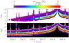 |
Fig. 9 Intensity response functions. Bottom: intensity response of individual wavelengths in Ca ii H to different layers of optical depth. Top: the former multiplied with the intensity spectrum transmitted by a broad-band filter (cf. Fig. 1). |
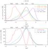 |
Fig. 10 Relative intensity response functions. Top panel: intensity response of synthetic Ca imaging data for filters with FWHM of 0.03 nm, 0.22 nm, 0.3 nm and 1 nm, respectively (red/orange/blue/purple lines). Green-dash-dotted line: intensity response for the FALF profile transmitted through a 0.3 nm filter. Black line: intensity response of the 630.25 nm line core. Bottom panel: response for a 0.3 nm filter and the 630.25 nm line core normalized to maximal response (blue/black line), and their difference (red line). |
We used the tabulated relation between optical depth and geometrical height of the Harvard Smithsonian Reference Atmosphere (Gingerich et al. 1971) to provide approximate formation heights in absolute geometrical units in contrast to a derivation of the height scale from the inversion results themselves, as done in Puschmann et al. (2005, 2010). The response function for the 1-nm-wide filter peaks at about 100 km, with a monotonically decreasing contribution from atmospheric layers above. The two broad-band Ca filters with 0.3 nm and 0.22 nm peak at about log τ = −2 (z ~ 200 km, similar to the 247 km obtained by Carlsson et al.2007) and have only small contributions from layers above log τ = −3. Their relative contributions reduce again monotonically with height in the atmosphere. The difference between transmitting the average observed Ca profile (blue line) or the synthetic FALF profile (green dash-dotted line) through a 0.3 nm filter is minor, even if the latter has a slightly larger contribution above log τ < − 3. A Lyot-type narrow-band filter, on the other hand, has significant contributions of layers up to 800 km, although the contribution peaks at about 600 km. The very line core of Ca ii H (line not drawn) would peak at the upper end of the optical depth scale, i.e. log τ = −6 (z ~ 1500 km), in the LTE approximation. The line core of the Fe i line at 630.25 nm behaves similar to, e.g., the 0.3 nm filter, but has a smaller contribution from upper atmospheric layers than this filter (Fig. 10). The contribution curves compare well with the visual appearance in Figs. 4 and 5: granular background pattern for the 1-nm-wide filter, inverse granulation at 0.22 to 0.3 nm, and absence of granulation for 0.03 nm. The relative contribution from heights above 800 km are 13, 4, 3 and about 1%, for a 0.03, 0.22, 0.3 and 1-nm-wide filter, respectively.
To determine where the difference intensity between the Fe line-core image and a 0.3-nm-wide filter originates from, we normalized these two response functions to their highest value instead of the total area. This allows one to roughly quantify the contribution height range of the difference image (lower panel of Fig. 10) because both functions peak at about the same height. The difference curve shows two local maxima at about 150 km and 400–500 km, respectively. About 11% of the difference originate from layers above 800 km, 67% from between 200 to 800 km and 16% from heights below 200 km. Thus both the response of a 0.3-nm-wide filter and the difference image between such a filter and a Fe line-core image have at maximum about 10% contribution from atmospheric layers above 800 km.
4. Summary and discussion
The interpretation of the broad-band (FWHM of 0.3 nm) Ca ii H filter imaging data of the Hinode Solar Optical Telescope (SOT) as a chromospheric measure, as done for example in Katsukawa et al. (2007), Mitra-Kraev et al. (2008), Pérez-Suárez et al. (2008), Guglielmino et al. (2008), Socas-Navarro et al. (2009), Yurchyshyn et al. (2010), Park & Chae (2012) or Gupta et al. (2013), requires that chromospheric layers dominate the total wavelength-integrated filter intensity. While beyond the solar limb this is ensured, the situation for observations on the solar disc is quite different. McIntosh & de Pontieu (2009) and de Pontieu et al. (2009) used a high-pass filter on Hinode Ca ii H imaging data, excluding frequencies below 18 mHz (periods > 60 s) to retain only what they called “upper chromospheric activity”. Characteristic intensity de-correlation times reach 60 secs already at heights of about 400 km (cf. Fig. 13 in Beck et al. 2008). Therefore, the effectiveness of such a high-pass filtering is not instantly clear. Reardon et al. (2009) found no good resemblance between broad-band Ca imaging and the line core of Ca ii IR spectra either on a temporal average or in their temporal evolution considering frequencies up to 15 mHz.
We found that the off-limb intensity in broad-band imaging data that can be attributed to upper chromospheric features such as spicules seen at heights of about 1 Mm or more above the limb is only about 5% of the intensity on the disc (Fig. 3). The off-limb intensity stems exclusively from emission in the line-core region of Ca ii H (cf. the average off-limb profiles in Beck & Rezaei 2011a) and Hϵ (cf. Appendix A) and cannot contain any contribution from photospheric radiation. This is, however, the result of an integration along a LOS roughly parallel to the solar limb, hence the solar surface, i.e. it adds up emission over an extended spatial distance at a roughly constant height in the atmosphere. The integrated intensity in the Ca line core for a LOS that is perpendicular to the solar surface will be significantly lower, but it requires a detailed calculation such as in Judge & Carlsson (2010) to accurately determine the amount. The investigation of the relative contribution of the Hϵ line at 397 nm to broad-band imaging shows that the line depth of the latter line in absorption on the disc for a vertical LOS is significantly lower than its amplitude of emission for a horizontal LOS. The total off-limb emission of 5% in the synthetic filter image thus is an upper limit for its contribution to a LOS at disc centre.
On the disc, on average only about 10% of the intensity that a broad-band filter transmits correspond to the line-core region (Fig. 1), which covers formation heights from the temperature minimum upwards. The maximal contribution of the line-core region of about 15% is attained at the centre of the magnetic network. Together with the off-limb filter intensity, this puts an upper limit of 15% as the maximal chromospheric, hence spicular, contribution to broad-band Ca filter imaging data at disc centre. The true spicular contribution to the broad-band filter imaging data could be quite overestimated by this. On the one hand, the complete Ca line-core region shows an increased intensity on magnetic locations – which are implicitly taken as locations of spicules here – which implies an increased temperature throughout all of the atmosphere, i.e. also at photospheric layers (Beck et al. 2008). On the other hand, the Ca line core at disc centre shows an absorption profile with overlaid emission, so it cannot be caused only by spicular emission. Since spicules exhibit emission profiles with about 5% of the intensity at the centre of the disc and the relative contribution of the line-core region to the total filter intensity to the filter is 15% at maximum, the effective contribution of spicules to a broad-band filter image could in reality be below 1% at disc centre. A similar estimate is provided by the intensity response function, where only about 3% of the relative contribution come from heights above 800 km for a 0.3-nm-wide filter.
A comparison with Ca line-core images, synthetic maps for various filter widths and temperature maps at different optical depth layers reveals that synthetic Ca broad-band imaging data match the line-core intensity of the photospheric Zeeman-sensitive Fe i line at 630.25 nm and the temperature at layers (far) below log τ = −4. The synthetic Ca broad-band imaging data lack the traces of fibrillar structures that appear in the Ca line-core intensity and LOS velocity above log τ = −4. Even a Lyot-type filter image shows at most weak indications of fibrillar structures. Imaging data with a 1-nm-wide Ca filter provide only information on solar atmospheric layers below the formation height of the line cores of photospheric lines (Figs. 4 and 10). It would thus be better to use some Lyot-type filter in the blue imaging channel of the GREGOR Fabry-Pérot Interferometer (Puschmann et al. 2012a,b,c) instead of such a broad filter in future observations. This would allow nearly chromospheric context imaging in addition to the photospheric spectropolarimetric data taken with the GFPI. The future integration of the Blue Imaging Solar Spectrometer (BLISS, Puschmann et al. 2012b, 2013) will then also allow the parallel recording of Ca ii H spectra at the 1.5 meter GREGOR telescope (Schmidt et al. 2012).
The intensity response function weighted by an average quiet-Sun Ca profile transmitted through a broad-band Ca filter locates the main contributions at about log τ = −2 (z ~ 200 km). The relative contribution reduces monotonically with height. A quantitative estimate of the formation height for the difference image between the line-core intensity of the Fe i line at 630.25 nm and broad-band Ca filter imaging has the strongest contributions between 200 and 800 km, and roughly equally strong contributions from above 800 km and below 200 km.
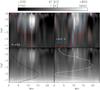 |
Fig. 11 Spatial cuts through temperature maps at disc centre. Bottom row: modulus of the temperature. Top row: relative temperature fluctuations after subtraction of the average temperature stratification. Left column: cut in y. Right column: cut in x. The black and white line in the bottom row indicate the response of a 0.3-nm-wide filter and the difference image of broad-band Ca imaging and Fe i line-core intensity, respectively. |
With a maximal contribution of about 10% for layers above 800 km, we therefore suggest that for observations at disc centre the broad-band Hinode Ca imaging data trace mainly upper photospheric layers (z ≪ 600 km) dominated by reverse granulation (cf. Figs. 4 and 5), but not upper chromospheric structures (z > 1 Mm), as was also concluded by RE09. A chromospheric contribution (z > 800 km) of up to 10% still does not allow one to use such data for studying the chromosphere at disc centre because it is impossible to isolate the corresponding information from the other 90% of contribution to the integrated intensity image.
Now, if the identification of the faint haze around the photospheric magnetic network with type II spicules in DW12 is thus strongly unlikely, the question remains what causes the haze instead. The results of the LTE inversion of the Ca ii H spectra provide a different possible explanation for the haze. Figure 11 shows the modulus of the temperature and the relative temperature variations on two spatial cuts across a network element (see also Fig. 16 of Beck et al. 2013b). The locations of the cuts are indicated by the white dashed lines in the temperature map at log τ = −5.1 of Fig. 8. Especially in the relative temperature fluctuations, a thermal canopy appears next to the photospheric flux concentrations located at x ~ 12 Mm in the left panel and at x ~ 10 Mm in the right panel. These thermal canopies extend up to a few Mm away from the location of the photospheric magnetic fields and appear at layers between log τ ~ − 3 up to − 6, which corresponds to heights between 500 – 600 km up to 2 Mm. Similar thermal canopies were recently identified by de la Cruz Rodríguez et al. (2013) in numerical simulations and observations of Ca ii IR spectra. With the location of the maximum intensity response below log τ = −4 (z ~ 600 km, bottom left panel of Fig. 11), the Hinode Ca imaging data are thus presumably sampling the lower end of these thermal canopies, which yield the haze around the photospheric magnetic network in the imaging data. The intensity response of the difference image of broad-band Ca imaging and photospheric Fe i line-core intensity peaks at the lower boundary of the thermal canopies (bottom right panel of Fig. 11).
5. Conclusions
The broad-band (FWHM ~ 0.3 nm) Ca filter imaging data of the Hinode SOT are dominated by upper photospheric layers (z < 600 km) in observations at disc centre. The faint haze of increased intensity around the photospheric network is most likely not related to entirely chromospheric structures such as spicules. We suggest that the haze instead traces thermal canopies below a height of 1 Mm that are related to concentrated photospheric magnetic flux. Any direct measurement of spicules with broad-band Ca filter imaging at disc centre should be impossible given the dominant intensity contribution (about 90%) of the line wings, hence photospheric layers to the intensity transmitted by a broad-band interference filter.
Online material
Appendix A: Contribution of Hϵ to the Hinode broad-band Ca filter
The 0.3-nm-wide Hinode Ca prefilter was selected to record intensity images from wavelengths around the Ca ii H line core. However, close to the Ca ii H line core at 396.85 nm, one can also find one of the Balmer lines, namely Hϵ at about 397 nm. Hϵ is a chromospheric line like Hα, but shows only a small line depth on the disc (cf. the on-disc spectra in the second panel from the top in Fig. A.1). Here we investigate the amount that emission in Hϵ contributes to off-limb data taken with a broad-band Ca prefilter.
The Ca ii H spectra recorded with the PCO 4000 camera cover a wider spectral range than the default POLIS Ca CCD. In addition to the data set on disc center used above, we also have some spectra near and beyond the limb taken on 30 June 2010 available (top panel of Fig. A.1). The stray-light correction for these data was made by subtracting a fraction of an average off-limb profile (cf. Martínez González et al. 2012), with the necessary fraction being determined from the residual intensity in the blue line wing far away from the chromospheric lines. The Hinode broad-band Ca prefilter extends far enough into the Ca line wing to also cover the chromospheric Hϵ line at 397 nm (middle two panels of Fig. A.1). Beyond the limb, the Hϵ line goes into emission. The amplitude of the Hϵ emission exceeds that of Ca ii H in some height range above the limb (d ~ 0 to 3 Mm; third panel from the top in Fig. A.1).
We estimated the relative contribution of Ca ii H and Hϵ to the total synthetic filter intensity for a 0.3-nm-wide prefilter centred on the Ca ii H line core by calculating the fraction of intensity that comes from the wavelength ranges marked in the top panel of Fig. A.1 (396.721 to 396.939 nm and 396.939 to 397.156 nm for Ca ii H and Hϵ, respectively). The contribution of Hϵ slightly exceeds that of Ca ii H (bottom panel of Fig. A.1) close to the limb (d ~ 0 Mm; >50% contribution). However, the stray-light correction included a step function with zero correction on the disc and full correction beyond the – manually set – limb position, so the results close to the assumed limb position (| d | < 0.3 Mm) might depend to some extent on the stray-light correction and the chosen limb location. Profiles at d ~ 1 Mm should have a clean and uncritical stray-light correction and therefore should be fully reliable. These profiles still show a larger emission amplitude in Hϵ than in Ca ii H (third panel from the top in Fig. A.1). The emission amplitude of Hϵ decreases faster with increasing limb distance than that of Ca ii H, which exceeds the former for d > 3 Mm. The relative contribution of Hϵ to the Hinode broad-band Ca filter decreases from about 50% at the limb to about 20% at d = 5 Mm and remains at this value for higher heights. For the typical height range of spicules (0 to 5–6 Mm), the relative contribution of Hϵ is about 1/3 of the total filter intensity. This contribution is significant and should be taken into account in any future detailed modelling of the Hinode Ca imaging data such as done in
Judge & Carlsson (2010), where Hϵ was not yet included. The Hϵ line is located in the wing of the filter transmission curve where its slope is steep, which makes the amount of transmitted intensity also sensitive to the Doppler shifts of Hϵ and not only to the amplitude of its emission.
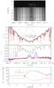 |
Fig. A.1 Relative contributions of Ca ii H and Hϵ to the intensity transmitted through the Hinode broad-band Ca filter. Top panel: average Ca ii H spectra near the limb. The vertical dotted and dashed lines denote the wavelength ranges attributed to Ca ii H and Hϵ, respectively. Second panel from the top: average observed on-disc (thick black line) and FTS spectrum (red line), and 0.3-nm-wide prefilter curve (dashed line, scaled arbitrarily). Third panel from the top: observed spectra at different limb distances. Bottom panel: relative contributions of Ca ii H (black line) and Hϵ (red line) to a 0.3-nm-wide prefilter. |
Sampling-limited spectral resolution.
Acknowledgments
The VTT is operated by the Kiepenheuer-Institut für Sonnenphysik (KIS) at the Spanish Observatorio del Teide of the Instituto de Astrofísica de Canarias (IAC). The POLIS instrument has been a joint development of the High Altitude Observatory (Boulder, USA) and the KIS. C.B. acknowledges partial support by the Spanish Ministry of Science and Innovation through project AYA2010–18029 and JCI-2009-04504. R.R. acknowledges financial support by the DFG grant RE 3282/1-1. We thank the referee for pointing out the importance of Hϵ to us.
References
- Barthol, P., Gandorfer, A., Solanki, S. K., et al. 2011, Sol. Phys., 268, 1 [NASA ADS] [CrossRef] [Google Scholar]
- Beck, C., & Rezaei, R. 2011a, A&A, 531, A173 [NASA ADS] [CrossRef] [EDP Sciences] [Google Scholar]
- Beck, C., & Rezaei, R. 2011b, VizieR Online Data Catalog: J/A+A/531/173 [Google Scholar]
- Beck, C., & Rezaei, R. 2012, in Magnetic Fields from the Photosphere to the Corona, eds. T. R. Rimmele, A. Tritschler, F. Wöger, et al., ASP Conf. Ser., 463, 257 [Google Scholar]
- Beck, C., Schmidt, W., Kentischer, T., & Elmore, D. 2005, A&A, 437, 1159 [NASA ADS] [CrossRef] [EDP Sciences] [Google Scholar]
- Beck, C., Mikurda, K., Bellot Rubio, L. R., Kentischer, T., & Collados, M. 2007, in Modern solar facilities – advanced solar science, eds. F. Kneer, K. G. Puschmann, & A. D. Wittmann, 55 [Google Scholar]
- Beck, C., Schmidt, W., Rezaei, R., & Rammacher, W. 2008, A&A, 479, 213 [NASA ADS] [CrossRef] [EDP Sciences] [Google Scholar]
- Beck, C., Khomenko, E., Rezaei, R., & Collados, M. 2009, A&A, 507, 453 (BE09) [NASA ADS] [CrossRef] [EDP Sciences] [Google Scholar]
- Beck, C., Rezaei, R., & Fabbian, D. 2011, A&A, 535, A129 [NASA ADS] [CrossRef] [EDP Sciences] [Google Scholar]
- Beck, C., Rezaei, R., & Puschmann, K. G. 2012, A&A, 544, A46 [NASA ADS] [CrossRef] [EDP Sciences] [Google Scholar]
- Beck, C., Rezaei, R., & Puschmann, K. G. 2013a, A&A, 549, A24 [NASA ADS] [CrossRef] [EDP Sciences] [Google Scholar]
- Beck, C., Rezaei, R., & Puschmann, K. G. 2013b, A&A, 553, A73 [NASA ADS] [EDP Sciences] [Google Scholar]
- Beckers, J. M. 1968, Sol. Phys., 3, 367 [NASA ADS] [Google Scholar]
- Bello González, N., & Kneer, F. 2008, A&A, 480, 265 [NASA ADS] [CrossRef] [EDP Sciences] [Google Scholar]
- Cabrera Solana, D., Bellot Rubio, L. R., & del Toro Iniesta, J. C. 2005, A&A, 439, 687 [NASA ADS] [CrossRef] [EDP Sciences] [Google Scholar]
- Carlsson, M., & Stein, R. F. 1997, ApJ, 481, 500 [Google Scholar]
- Carlsson, M., Hansteen, V. H., de Pontieu, B., et al. 2007, PASJ, 59, 663 [NASA ADS] [CrossRef] [Google Scholar]
- de la Cruz Rodríguez, J., & Socas-Navarro, H. 2011, A&A, 527, L8 [NASA ADS] [CrossRef] [EDP Sciences] [Google Scholar]
- de la Cruz Rodríguez, J., de Pontieu, B., Carlsson, M., & Rouppe van der Voort, L. H. M. 2013, ApJ, 764, L11 [NASA ADS] [CrossRef] [Google Scholar]
- de Pontieu, B., McIntosh, S., Hansteen, V. H., et al. 2007, PASJ, 59, 655 [Google Scholar]
- de Pontieu, B., McIntosh, S. W., Hansteen, V. H., & Schrijver, C. J. 2009, ApJ, 701, L1 [NASA ADS] [CrossRef] [Google Scholar]
- de Wijn, A. G. 2012, ApJ, 757, L17 (DW12) [NASA ADS] [CrossRef] [Google Scholar]
- Fontenla, J. M., Avrett, E., Thuillier, G., & Harder, J. 2006, ApJ, 639, 441 [NASA ADS] [CrossRef] [Google Scholar]
- Gingerich, O., Noyes, R. W., Kalkofen, W., & Cuny, Y. 1971, Sol. Phys., 18, 347 [NASA ADS] [CrossRef] [Google Scholar]
- Guglielmino, S. L., Zuccarello, F., Romano, P., & Bellot Rubio, L. R. 2008, ApJ, 688, L111 [NASA ADS] [CrossRef] [Google Scholar]
- Gupta, G. R., Subramanian, S., Banerjee, D., Madjarska, M. S., & Doyle, J. G. 2013, Sol. Phys., 282, 67 [NASA ADS] [CrossRef] [Google Scholar]
- Jafarzadeh, S., Solanki, S. K., Feller, A., et al. 2013, A&A, 549, A116 [NASA ADS] [CrossRef] [EDP Sciences] [Google Scholar]
- Judge, P. G., & Carlsson, M. 2010, ApJ, 719, 469 [NASA ADS] [CrossRef] [Google Scholar]
- Judge, P. G., Tritschler, A., & Chye Low, B. 2011, ApJ, 730, L4 [NASA ADS] [CrossRef] [Google Scholar]
- Katsukawa, Y., Berger, T. E., Ichimoto, K., et al. 2007, Science, 318, 1594 [NASA ADS] [CrossRef] [Google Scholar]
- Kentischer, T. J. 1995, A&AS, 109, 553 [NASA ADS] [Google Scholar]
- Kentischer, T. J., Schmidt, W., Sigwarth, M., & von Uexküll, M. 1998, A&A, 340, 569 [NASA ADS] [Google Scholar]
- Kosugi, T., Matsuzaki, K., Sakao, T., et al. 2007, Sol. Phys., 243, 3 [NASA ADS] [CrossRef] [Google Scholar]
- Langangen, Ø., de Pontieu, B., Carlsson, M., et al. 2008, ApJ, 679, L167 [NASA ADS] [CrossRef] [Google Scholar]
- Lyot, B. 1944, Ann. Astrophys., 7, 31 [NASA ADS] [Google Scholar]
- Marsh, K. A. 1976, Sol. Phys., 50, 37 [NASA ADS] [CrossRef] [Google Scholar]
- Martínez González, M. J., Asensio Ramos, A., Manso Sainz, R., Beck, C., & Belluzzi, L. 2012, ApJ, 759, 16 [NASA ADS] [CrossRef] [Google Scholar]
- McIntosh, S. W., & de Pontieu, B. 2009, ApJ, 706, L80 [NASA ADS] [CrossRef] [Google Scholar]
- Mitra-Kraev, U., Kosovichev, A. G., & Sekii, T. 2008, A&A, 481, L1 [NASA ADS] [CrossRef] [EDP Sciences] [Google Scholar]
- Öhman, Y. 1938, Nature, 141, 157 [NASA ADS] [CrossRef] [Google Scholar]
- Park, S., & Chae, J. 2012, Sol. Phys., 280, 103 [NASA ADS] [CrossRef] [Google Scholar]
- Pérez-Suárez, D., Maclean, R. C., Doyle, J. G., & Madjarska, M. S. 2008, A&A, 492, 575 [NASA ADS] [CrossRef] [EDP Sciences] [Google Scholar]
- Pietarila, A., Hirzberger, J., Zakharov, V., & Solanki, S. K. 2009, A&A, 502, 647 [NASA ADS] [CrossRef] [EDP Sciences] [Google Scholar]
- Puschmann, K. G., & Beck, C. 2011, A&A, 533, A21 [NASA ADS] [CrossRef] [EDP Sciences] [Google Scholar]
- Puschmann, K. G., & Sailer, M. 2006, A&A, 454, 1011 [NASA ADS] [CrossRef] [EDP Sciences] [Google Scholar]
- Puschmann, K. G., Ruiz Cobo, B., Vázquez, M., Bonet, J. A., & Hanslmeier, A. 2005, A&A, 441, 1157 [NASA ADS] [CrossRef] [EDP Sciences] [Google Scholar]
- Puschmann, K. G., Kneer, F., Seelemann, T., & Wittmann, A. D. 2006, A&A, 451, 1151 [NASA ADS] [CrossRef] [EDP Sciences] [Google Scholar]
- Puschmann, K. G., Kneer, F., & Domínguez Cerdeña, I. 2007, in Modern solar facilities – advanced solar science, eds. F. Kneer, K. G. Puschmann, & A. D. Wittmann (Universitätsverlag Göttingen), 151 [Google Scholar]
- Puschmann, K. G., Ruiz Cobo, B., & Martínez Pillet, V. 2010, ApJ, 720, 1417 [NASA ADS] [CrossRef] [Google Scholar]
- Puschmann, K. G., Balthasar, H., Bauer, S.-M., et al. 2012a, in Magnetic Fields from the Photosphere to the Corona, eds. T. R. Rimmele, A. Tritschler, F. Wöger, et al., ASP Conf. Ser., 463, 423 [NASA ADS] [Google Scholar]
- Puschmann, K. G., Balthasar, H., Beck, C., et al. 2012b, in Ground-based and Airborne Instrumentation for Astronomy IV, SPIE Conf. Ser., 8446, 79 [Google Scholar]
- Puschmann, K. G., Denker, C., Kneer, F., et al. 2012c, Astron. Nachr., 333, 880 [NASA ADS] [Google Scholar]
- Puschmann, K. G., Denker, C., Balthasar, H., et al. 2013, Opt. Eng. 52 (8), 081606 [Google Scholar]
- Rammacher, W., & Ulmschneider, P. 1992, A&A, 253, 586 [NASA ADS] [Google Scholar]
- Reardon, K. P., Uitenbroek, H., & Cauzzi, G. 2009, A&A, 500, 1239 (RE09) [NASA ADS] [CrossRef] [EDP Sciences] [Google Scholar]
- Rezaei, R., Schlichenmaier, R., Beck, C. A. R., Bruls, J. H. M. J., & Schmidt, W. 2007, A&A, 466, 1131 [NASA ADS] [CrossRef] [EDP Sciences] [Google Scholar]
- Rezaei, R., Bruls, J. H. M. J., Schmidt, W., et al. 2008, A&A, 484, 503 [NASA ADS] [CrossRef] [EDP Sciences] [Google Scholar]
- Rouppe van der Voort, L., Leenaarts, J., de Pontieu, B., Carlsson, M., & Vissers, G. 2009, ApJ, 705, 272 [NASA ADS] [CrossRef] [Google Scholar]
- Rutten, R. J., & Uitenbroek, H. 1991, Sol. Phys., 134, 15 [NASA ADS] [CrossRef] [Google Scholar]
- Schmidt, W., von der Lühe, O., Volkmer, R., et al. 2012, Astron. Nachr., 333, 796 [NASA ADS] [CrossRef] [Google Scholar]
- Schröter, E. H., Soltau, D., & Wiehr, E. 1985, Vistas Astron., 28, 519 [Google Scholar]
- Sekse, D. H., Rouppe van der Voort, L., & de Pontieu, B. 2012, ApJ, 752, 108 [NASA ADS] [CrossRef] [Google Scholar]
- Skomorovsky, V. I., Kushtal, G. I., & Sadokhin, V. P. 2012, in Ground-based and Airborne Instrumentation for Astronomy IV, SPIE Conf. Ser., 8446 [Google Scholar]
- Socas-Navarro, H., McIntosh, S. W., Centeno, R., de Wijn, A. G., & Lites, B. W. 2009, ApJ, 696, 1683 [NASA ADS] [CrossRef] [Google Scholar]
- Sterling, A. C. 2000, Sol. Phys., 196, 79 [NASA ADS] [CrossRef] [Google Scholar]
- Sterling, A. C., Moore, R. L., & DeForest, C. E. 2010, ApJ, 714, L1 [NASA ADS] [CrossRef] [Google Scholar]
- Tritschler, A., Schmidt, W., Langhans, K., & Kentischer, T. 2002, Sol. Phys., 211, 17 [NASA ADS] [CrossRef] [Google Scholar]
- Tsuneta, S., Ichimoto, K., Katsukawa, Y., et al. 2008, Sol. Phys., 249, 167 [NASA ADS] [CrossRef] [Google Scholar]
- Uitenbroek, H. 2000, ApJ, 536, 481 [NASA ADS] [CrossRef] [Google Scholar]
- van Noort, M., Rouppe van der Voort, L., & Löfdahl, M. G. 2005, Sol. Phys., 228, 191 [NASA ADS] [CrossRef] [Google Scholar]
- Wang, J., Ai, G., Song, G., et al. 1995, Sol. Phys., 161, 229 [NASA ADS] [CrossRef] [Google Scholar]
- Yurchyshyn, V. B., Goode, P. R., Abramenko, V. I., et al. 2010, ApJ, 722, 1970 [NASA ADS] [CrossRef] [Google Scholar]
- Zirin, H. 1974, Sol. Phys., 38, 91 [NASA ADS] [CrossRef] [Google Scholar]
All Figures
|
Fig. 1 Average observed and theoretical Ca profiles with different filters. Top panel: average observed Ca profile at disc centre (black line). Purple/blue/orange/red dashed lines: Gaussians with FWHM of 1 nm, 0.3 nm, 0.22 nm, and 0.03 nm, respectively, centred at 396.85 nm. Purple/blue/orange/red solid lines: multiplication of the observed profile with the filter transmission. Bottom panel: multiplication of NLTE FALC/FALF profiles (blue-dash-triple-dotted/red-dash-dotted lines) with a 0.3 nm filter. |
| In the text | |
|
Fig. 2 Overview of the observations at the solar limb. Top panel, left to right: 2D maps obtained from the spectra in the outer wing (OW), the line core (Icore, linear display), the synthetic Ca broad-band imaging data (linear display), and the same in logarithmic and clipped display. Bottom panel, left to right: contrast-enhanced Ca ii K Lyot-filter and Hinode Ca ii H broad-band filter images at the solar limb. |
| In the text | |
|
Fig. 3 Intensity and relative core contribution on radial cuts normalized to the intensity at disc centre. Top panel: average intensity in OW (red line), Ca line core Icore (blue line) and synthetic Ca broad-band imaging data (black line). Bottom panel: relative contribution of the line core to the broad-band filter intensity. The dashed vertical lines denote the location of the limb. |
| In the text | |
|
Fig. 4 Disc centre observations with different filter widths. Top row, left to right: Ca ii K Lyot image (0.03 nm), Hinode/FG broad-band Ca ii H image (0.3 nm), MFBD-reconstructed Ca image (1 nm), co-spatial MOMFBD line-core image of Fe i at 630.25 nm and the unsigned wavelength-integrated Stokes V signal of this line recorded with the GFPI. Bottom row, left to right: synthetic images derived by applying the corresponding filters of the top row to Ca spectra observed at disc centre. The synthetic image for the 1-nm-wide filter was obtained from the Ca spectra taken with a PCO camera inside of POLIS at a different time. All images are scaled individually inside their full dynamical range. |
| In the text | |
|
Fig. 5 Overview maps of the POLIS observation at disc centre. Bottom row, left to right: OW, Icore of Ca ii H and Stokes | V | signal of the Fe i line 630.25 nm. Top row, left to right: Icore of Fe i at 630.25 nm, synthetic Ca broad-band imaging data and difference image of the latter two. The dotted white lines denote the locations of the cuts shown in Fig. 6. |
| In the text | |
|
Fig. 6 Cuts along the dotted white lines in Fig. 5 through the Fe line-core map (black lines), the synthetic Ca broad-band imaging (red lines) and the Ca line-core intensity map (blue lines). All intensities have been re-scaled to the same dynamical range by linear regression. The black rectangles mark locations of network and their surroundings. |
| In the text | |
|
Fig. 7 Relative contribution of the line core to the filter intensity at the disc centre. Left/right panel: for filters of FWHM = 0.22 and 0.3 nm, respectively. |
| In the text | |
|
Fig. 8 Temperature maps at disc centre. Bottom row, left to right: at optical depths of log τ = −0.6, − 1.6, and − 3.6. Top row, left to right: at log τ = −5.1, and averaged over − 0.6 to − 5.1. The top rightmost panel shows the synthetic Ca broad-band image. The white dashed lines in the temperature map at log τ = −5.1 denote the locations of the spatial cuts shown in Fig. 11. |
| In the text | |
|
Fig. 9 Intensity response functions. Bottom: intensity response of individual wavelengths in Ca ii H to different layers of optical depth. Top: the former multiplied with the intensity spectrum transmitted by a broad-band filter (cf. Fig. 1). |
| In the text | |
|
Fig. 10 Relative intensity response functions. Top panel: intensity response of synthetic Ca imaging data for filters with FWHM of 0.03 nm, 0.22 nm, 0.3 nm and 1 nm, respectively (red/orange/blue/purple lines). Green-dash-dotted line: intensity response for the FALF profile transmitted through a 0.3 nm filter. Black line: intensity response of the 630.25 nm line core. Bottom panel: response for a 0.3 nm filter and the 630.25 nm line core normalized to maximal response (blue/black line), and their difference (red line). |
| In the text | |
|
Fig. 11 Spatial cuts through temperature maps at disc centre. Bottom row: modulus of the temperature. Top row: relative temperature fluctuations after subtraction of the average temperature stratification. Left column: cut in y. Right column: cut in x. The black and white line in the bottom row indicate the response of a 0.3-nm-wide filter and the difference image of broad-band Ca imaging and Fe i line-core intensity, respectively. |
| In the text | |
|
Fig. A.1 Relative contributions of Ca ii H and Hϵ to the intensity transmitted through the Hinode broad-band Ca filter. Top panel: average Ca ii H spectra near the limb. The vertical dotted and dashed lines denote the wavelength ranges attributed to Ca ii H and Hϵ, respectively. Second panel from the top: average observed on-disc (thick black line) and FTS spectrum (red line), and 0.3-nm-wide prefilter curve (dashed line, scaled arbitrarily). Third panel from the top: observed spectra at different limb distances. Bottom panel: relative contributions of Ca ii H (black line) and Hϵ (red line) to a 0.3-nm-wide prefilter. |
| In the text | |
Current usage metrics show cumulative count of Article Views (full-text article views including HTML views, PDF and ePub downloads, according to the available data) and Abstracts Views on Vision4Press platform.
Data correspond to usage on the plateform after 2015. The current usage metrics is available 48-96 hours after online publication and is updated daily on week days.
Initial download of the metrics may take a while.