| Issue |
A&A
Volume 551, March 2013
|
|
|---|---|---|
| Article Number | A38 | |
| Number of page(s) | 22 | |
| Section | Interstellar and circumstellar matter | |
| DOI | https://doi.org/10.1051/0004-6361/201117161 | |
| Published online | 18 February 2013 | |
Ortho-H2 and the age of prestellar cores⋆
1
LERMA, UMR 8112 du CNRS, Observatoire de Paris, 61, Av. de
l′Observatoire,
75014
Paris,
France
e-mail: This email address is being protected from spambots. You need JavaScript enabled to view it.
2
LERMA, UMR 8112 du CNRS, Ecole Normale Supérieure, 24 rue Lhomond,
75231
Paris Cedex 05,
France
3
Institut de Chimie des Milieux et des Matériaux de Poitiers, UMR
CNRS 6503, Université de Poitiers, 86022
Poitiers Cedex,
France
4
Laboratoire Interdisciplinaire Carnot de Bourgogne, UMR 6303 du
CNRS, Université de Bourgogne, 21078
Dijon Cedex,
France
5
UFR Sciences et Techniques, Université de Franche-Comté,
25030
Besançon Cedex,
France
6
Instituto de Física Fundamental, CSIC, Serrano 123, 28006
Madrid,
Spain
7
Institut de Planétologie et d’Astrophysique de Grenoble, UMR 5274
du CNRS, Université Joseph Fourier, BP 53, 38041
Grenoble Cedex 09,
France
Received:
29
April
2011
Accepted:
28
November
2012
Abstract
Prestellar cores form from the contraction of cold gas and dust material in dark clouds before they collapse to form protostars. Several concurrent theories exist to describe this contraction but they are currently difficult to distinguish. One major difference is the timescale involved in forming the prestellar cores: some theories advocate nearly free-fall speed via, e.g., rapid turbulence decay, while others can accommodate much longer periods to let the gas accumulate via, e.g., ambipolar diffusion. To tell the difference between these theories, measuring the age of prestellar cores could greatly help. However, no reliable clock currently exists. We present a simple chemical clock based on the regulation of the deuteration by the abundance of ortho–H2 that slowly decays away from the ortho-para statistical ratio of 3 down to or less than 0.001. We use a chemical network fully coupled to a hydrodynamical model that follows the contraction of a cloud, starting from uniform density, and reaches a density profile typical of a prestellar core. We compute the N2D+/N2H+ ratio along the density profile. The disappearance of ortho-H2 is tied to the duration of the contraction and the N2D+/N2H+ ratio increases in the wake of the ortho-H2 abundance decrease. By adjusting the time of contraction, we obtain different deuteration profiles that we can compare to the observations. Our model can test fast contractions (from 104 to 106 cm-3 in ~0.5 My) and slow contractions (from 104 to 106 cm-3 in ~5 My). We have tested the sensitivity of the models to various initial conditions. The slow-contraction deuteration profile is approximately insensitive to these variations, while the fast-contraction deuteration profile shows significant variations. We found that, in all cases, the deuteration profile remains clearly distinguishable whether it comes from the fast collapse or the slow collapse. We also study the para-D2H+/ortho-H2D+ ratio and find that its variation is not monotonic, so it does not discriminate between models. Applying this model to L183 (=L134N), we find that the N2D+/N2H+ ratio would be higher than unity for evolutionary timescales of a few megayears independently of other parameters, such as cosmic ray ionization rate or grain size (within reasonable ranges). A good fit to the observations is only obtained for fast contraction (≤0.7 My from the beginning of the contraction and ≤4 My from the birth of the molecular cloud based on the need to keep a high ortho-H2 abundance when the contraction starts – ortho-H2/para-H2 ≥ 0.2 – to match the observations). This chemical clock therefore rules out slow contraction in L183 and steady-state chemical models, since steady state is clearly not reached here. This clock should be applied to other cores to help distinguish slow and fast contraction theories over a large sample of cases.
Key words: astrochemistry / evolution / ISM: clouds / ISM: molecules / ISM: individual objects: L183 / ISM: abundances
Appendices are available in electronic form at http://www.aanda.org
© ESO, 2013
1. Introduction
Star formation is one of the fundamental problems astrophysics has been tackling ever since it exists. It has subdivided into two or even three branches by recognizing that low mass, intermediate mass and high mass star formations take different paths. Among the three, the low-mass star formation process is understood the best, because there are many more low-mass stars than high-mass stars, therefore there are a number of low-mass star-forming regions close to us that can be studied in detail. However, details of the first steps of this low-mass star formation remain uncertain. What causes the contraction of the prestellar core and its subsequent collapse? Is contraction due to supersonic turbulence fast decay or to slow ambipolar diffusion in a magnetically subcritical cloud? Which initial or evolving conditions set up the final mass of a star? How do multiple systems form? All these questions have been asked long ago and are still present.
It is obviously difficult to measure constraining parameters, such as the magnetic field intensity, the cosmic ray ionization rate, and its partly related dark cloud electronic abundance, which would help for assessing the importance of ambipolar diffusion (see however Crutcher et al. 2010). Because the different prestellar core-making theories imply different timescales, by a factor up to 10, measuring the age of the cores could help distinguish slow and fast theories. Until now, such clocks have not been found. In principle, chemical clocks could be used because many species appear with different timescales: SO and NH3 take at least 1 My to appear, while CS peak abundance is reached ten times faster (Roberts et al. 2004; Flower et al. 2006a), and the SO/CS ratio could be considered as such a clock. Nilsson et al. (2000) have shown, however, that this ratio depended on multiple factors, time evolution being only one of them, and other conditions such as the initial O/C+ ratio would strongly influence the result making the SO/CS ratio an unreliable clock if the other parameters cannot be estimated with some accuracy. The existence of chemical clocks has not yet been established (van Weeren et al. 2009) but the situation is now evolving: we recently presented a chemical model that clearly constrains the age of molecular clouds below 10 My (Pagani et al. 2011).
Recently, we suggested two new clocks to measure the age of prestellar cores (Pagani et al. 2009, 2010b). One is linked to the direct detection and measurement of grown grains in dark clouds (the coreshine effect, Steinacker et al. 2010), which we have shown to be feasible in many clouds (Pagani et al. 2010b). These big grains have built up from interstellar standard grains, and by applying a growth model such as those of Ormel et al. (2009), it should be possible to determine the age of the cloud. As a first example, we made a simple application of the coreshine effect to study the age of clouds in the Gum/Vela region (Pagani et al. 2012b). The other one is linked to chemistry but in a particular case where the chemistry is simple and the initial conditions known or of limited influence. The chemistry is the one that appears in depleted cores where all heavy species have disappeared, including CO (e.g. Caselli et al. 1999; Bergin et al. 2002; Bacmann et al. 2002; Tafalla et al. 2004; Pagani et al. 2005; Ford & Shirley 2011). These depleted cores are well-known for displaying large deuterium enhancements because the deuterium chemistry is greatly favoured once CO has disappeared, as illustrated by the detection of H2D+ itself (e.g. Caselli et al. 2003; Vastel et al. 2006; Caselli et al. 2008; Pagani et al. 2009, hereafter P09), D2H+ (Vastel et al. 2004; Parise et al. 2011) or improbable triply deuterated species like ND3 (Lis et al. 2002; Tak et al. 2002) and CD3OH (Parise et al. 2004).
This chemistry depends not only on the shrinkage of CO probably by two to three orders of
magnitude, but also on the disappearance of ortho-H2. The importance of the
ortho/para spin states of H2 in the deuterium chemistry was first invoked by
Pineau des Forêts et al. (1991), but considering
only para-H2D+. The role of o-H2 on the ortho/para
H2D+ ratio was discussed in detail for the first time by Pagani et al. (1992) and was subsequently expanded to
include D2H+ and  by Flower et al. (2004, 2006b). In P09, we updated the Flower et al.
(2004) chemical model with the complete set of rates involving ortho and para
states of H2,
by Flower et al. (2004, 2006b). In P09, we updated the Flower et al.
(2004) chemical model with the complete set of rates involving ortho and para
states of H2,  and their
isotopologues, as estimated by Hugo et al. (2009).
Sipilä et al. (2010) and Parise et al. (2011) have since developed similar models but the former
focused their studies on the steady-state case, while the latter conclude that the
steady-state case gave a better fit than earlier times. In P09, we assumed full depletion of
heavy species except for N2 and CO whose abundance was a free parameter of the
model. We applied it to reproduce the abundance profile of ortho-H2D+
and the N2D+/N2H+ ratio profile across the
L183 (also known as L134N) main prestellar core that had been derived from the observations of
these species (Pagani et al. 2007). We noted that the
profile could be fitted but that the time needed to reach the observed ratio for each layer
was negatively correlated with its density. Since the evolution speed of chemistry depends
on the collision rate between species which in turn depends on the density of the medium,
the result could be explained by the density gradient along the core. Consequently, it
appeared that the time discrepancy would be solved if the core had not always been as
observed today but started with a lower and probably relatively uniform density and
contracted to its present state. The central part that becomes the denser would evolve
faster and therefore farther than the outer layers in the same time period but not as fast
as if it had always been at the 106 cm-3 level. The conclusion was
that the model was giving a lower limit to the age of the contracting core and that this
limit was set by the slowest evolving layer, i.e., the most external one, with the lowest
density. This lower limit was 2 × 10⁵ years, therefore compatible with even a
free-fall time (~0.5 My for a density of 104 cm-3). Fast contraction
could not be ruled out. Such a lower limit is not particularly useful, however, and a model
that includes both the dynamical evolution and the chemistry is needed to better determine
the age of the prestellar core. We therefore used the chemical model of P09 in the 1 D
chemical and hydrodynamical model of Lesaffre et al.
(2005) to try to follow the deuteration amplification through the density increase
of a model core. We report here the general predictions of this new model and its
application to the L183 case. Though no quantitative estimates were given, it must be noted
that Caselli (2002) has already shown that the
N2D+/N2H+ ratio would increase with the age of
the prestellar core and its collapse advancement.
and their
isotopologues, as estimated by Hugo et al. (2009).
Sipilä et al. (2010) and Parise et al. (2011) have since developed similar models but the former
focused their studies on the steady-state case, while the latter conclude that the
steady-state case gave a better fit than earlier times. In P09, we assumed full depletion of
heavy species except for N2 and CO whose abundance was a free parameter of the
model. We applied it to reproduce the abundance profile of ortho-H2D+
and the N2D+/N2H+ ratio profile across the
L183 (also known as L134N) main prestellar core that had been derived from the observations of
these species (Pagani et al. 2007). We noted that the
profile could be fitted but that the time needed to reach the observed ratio for each layer
was negatively correlated with its density. Since the evolution speed of chemistry depends
on the collision rate between species which in turn depends on the density of the medium,
the result could be explained by the density gradient along the core. Consequently, it
appeared that the time discrepancy would be solved if the core had not always been as
observed today but started with a lower and probably relatively uniform density and
contracted to its present state. The central part that becomes the denser would evolve
faster and therefore farther than the outer layers in the same time period but not as fast
as if it had always been at the 106 cm-3 level. The conclusion was
that the model was giving a lower limit to the age of the contracting core and that this
limit was set by the slowest evolving layer, i.e., the most external one, with the lowest
density. This lower limit was 2 × 10⁵ years, therefore compatible with even a
free-fall time (~0.5 My for a density of 104 cm-3). Fast contraction
could not be ruled out. Such a lower limit is not particularly useful, however, and a model
that includes both the dynamical evolution and the chemistry is needed to better determine
the age of the prestellar core. We therefore used the chemical model of P09 in the 1 D
chemical and hydrodynamical model of Lesaffre et al.
(2005) to try to follow the deuteration amplification through the density increase
of a model core. We report here the general predictions of this new model and its
application to the L183 case. Though no quantitative estimates were given, it must be noted
that Caselli (2002) has already shown that the
N2D+/N2H+ ratio would increase with the age of
the prestellar core and its collapse advancement.
In Sect. 2, we discuss the chemical clock scheme. In Sect. 3, we briefly present the model. In Sect. 4, we discuss the role of ortho-H2, its abundance and evolution in the cloud prior to the prestellar core formation, and in Sect. 5, we show the predictions upon the N2D+/N2H+ ratio profile depending on different initial conditions or rates. In Sect. 6, we analyse the conditions that best reproduce the L183 observations and present our conclusions in Sect. 7. Three appendices are added, the first one (A) shows the impact of the new ortho-to-para H2 conversion rate (presented in Sect. 4), the second one (B) presents a similar study to Sect. 5 but centred on the para-D2H+/ortho-H2D+ ratio, and the third one (C) compiles some useful chemical reaction rates.
2. The chemical clock
One of the main problems with chemical clocks is our ignorance of the initial conditions especially the abundance of the various species in the gas phase. Apart from H2, HD (but see Bell et al. 2011, for a discussion on its fluctuations due to turbulence), and possibly CO, which seems to reach an abundance close to X[CO] = CO/H2 ≈ 1–2 × 10⁻⁴ in most clouds if not depleted, all other species’ abundances are difficult to model without knowing the initial conditions (see Liszt 2009, for a recent discussion of initial conditions).
A second problem is to retrieve the distribution along the line of sight of the observed species to account for density and temperature variations, chemical fluctuations and possibly depletion effects. In this respect, line of sight-averaged depletion measurements of CO are merely a measurement of the size of the undepleted region compared to the size of the depleted core (as soon as CO abundance drops in the core, its contribution to the total CO line intensity becomes unmeasurable directly, as discussed in e.g. Pagani et al. 2005, 2010a), and the correlation between CO depletion and deuterium enrichment obtained with this simple method is not reliable.
Here, we reduce the number of free parameters by considering the ratio of two species with common reactants and by considering the variation of this ratio along a prestellar core profile for which a 1D symmetry is a relatively good approximation. These two species, N2H+ and N2D+ (known as diazenylium and deuterated diazenylium), have N2 as a common parent and their production and destruction follow similar routes. They are also confined to the depleted core of the cloud, and therefore the physical conditions are relatively well-known and the chemistry is simple. There is no line-of-sight interference with other parts of the cloud since these species are readily destroyed by CO when the latter is abundant, and N2 is also relatively slow to form, thus delaying its appearance in the low-density parts of the cloud (Flower et al. 2006a). Therefore these species remain absent from the rest of the cloud (a similar work with DCO+ and HCO+ would be impossible because of the widespread presence of HCO+. See also Caselli 2002, for another discussion of the comparative benefits of N2D+ versus DCO+). While it is easy to model a given abundance for any of these two species (N2D+ and N2H+), they both depend on the unmeasurable abundance of N2, hence their ratio is independent of this unknown quantity and remains a more constraining quantity to match. This ratio alone is however not sufficient to distinguish different models. For each model, we can most often find a solution to match any single ratio. Because the density changes with time and because the chemistry evolution speed depends upon the actual density, the N2D+/N2H+ ratio profile along the density profile is sensitive to the history of the contraction of the cloud as explained in the Introduction and shown with the preliminary results of P09. Therefore the outcome depends on the collapse duration as long as the chemistry has not reached its steady state. Indeed P09 has shown that the N2D+/N2H+ steady state ratios are much higher than the observed ratios in the case of L183 (their Fig. 7) and therefore discrimination is possible.
Initial conditions are not a difficulty in this model apart from the initial H2 OPR, which is not known. The abundance of N2 need not be strictly homogeneous because this should not change the diazenylium ratio, and both diazenylium isotopologues are undetectable before the contraction starts because CO has not depleted yet. As noted above CO efficiently destroys both species. A spectacular such example is reported in Pagani et al. (2010a). Moreover, all the initial conditions are probably homogeneous enough in the region of interest at the beginning of the contraction when the density is relatively low and uniform. Thus, the variation in the diazenylium ratio profile should solely trace the chemical evolution from the beginning of the contraction.
Apart from density, the chemistry evolution speed itself depends on several conditions, which we list below.
-
1.
The H2 OPR at the start. This could be the only problematic initial condition. The lower the ratio, the faster the deuteration of diazenylium occurs.
-
2.
The grain size. The bigger the grains, the less numerous they are and the recombination of H+ (and somewhat
) on
negatively charged grains is less efficient in removing H+ from the gas
phase. In turn, a larger abundance of H+ allows a faster conversion of
ortho-H2 into para-H2 (Gerlich
1990) and an acceleration of the deuteration of diazenylium. -
3.
The cosmic ray ionization rate. The higher the rate, the higher the production of H+ and
, both
converters of ortho-H2 in para-H2. On the whole, a higher
ionization rate means a proportional acceleration of the chemistry.
All these parameters are tested and discussed below, and we will show that, for any reasonable value, they do not change our conclusions.
Because the deuteration of diazenylium relies upon the abundance of the deuterated
isotopologues of , it could be
interesting to also investigate the abundance of these isotopologues. Owing to the paucity
of the observable transitions from the ground (one ground transition for
ortho-H2D+ and one ground transition for
para-D2H+) and the uncertainty on collisional coefficients (Hugo et al. 2009), studying them is, however, much more
difficult. For the sake of completeness, we present in Appendix B the results of our model for the
para-D2H+/ortho-H2D+ ratio in a similar
fashion to those of N2D+/N2H+, which we present
in Sect. 5.
3. Numerical method
The code we use is described in detail in Lesaffre et al. (2005). It solves the equations of hydrodynamics coupled to cooling, chemistry and simplified radiative transfer on grains. The system is 1D with spherical geometry. In the present study, it is discretized with 200 Lagrangian zones that are initially logarithmically spaced in radius.
The starting conditions of our simulations are a homogeneous sphere with uniform composition, size 0.1 pc (=20 000 AU), and mass 1 M⊙. As the system tries to relax to a stable Bonnor-Ebert configuration, the external pressure is continuously increased, which eventually leads to gravitational collapse. We stop the computation when the central H nuclei density reaches ~106 cm-3, which corresponds to the typical prestellar core central densities.
As the cloud first relaxes towards hydrostatic equilibrium, it experiences a few rebounds. On some occasions, these rebounds can trigger spherically convergent shocks that stall the code as they asymptotically reach the centre. To avoid this unwanted transient behaviour, we make use of an additional friction term in the velocity equation. The timescale for this friction is 10 My, which is short enough to avoid the unwanted shocks but long enough so that it does not affect the collapse.
The chemical network used in Lesaffre et al. (2005)
was mainly designed to account for the major coolants (CO, H2O, OH,
H2) of the multiphase interstellar medium with a minimum number of reactions
(120 reactions and 35 species). However, in the present study, we limit the computation to
the early phases of the collapse which experience very low temperatures around 10 K. In
these conditions, CO remains the only efficient coolant and we are thus free to reduce the
cooling-motivated part of our network to the simple reactions of adsorption and desorption
of the CO molecule. We then incorporate the full deuteration network of P09 and extend it to
include reactions with atomic D that were neglected in P09, unlike all the other models
derived from Walmsley et al. (2004), which do include
these reactions. These reactions with D (such as + D →
H2D+ + H) have a sizeable influence mostly at steady state when
atomic deuterium becomes important. In P09, we concentrate on a 7 K gas for which we
computed all the rates we needed or selected them in tables. Since the temperature is
self-consistently evaluated here (see below), we have to replace tabulated coefficients with
Kooij/Arrhenius expressions
(k = α(T/300)βe−γ/T cm3 s-1
where T is the temperature in Kelvin and α,β, and
γ the coefficients to be adjusted to fit the tabulated values) to be able
to follow the evolution of the chemical rates with temperature. This concerns all of the
Hugo reaction rates (Hugo et al. 2009, values are
fitted only between 5 and 20 K in this paper) and the dissociative recombination rates from
P09. They are given in Appendix C. CO is either a
constant (free) parameter or its time-dependent depletion/desorption is taken into account
(see Sect. 5.3.3; note that the N2
abundance is still kept constant as an adjustable parameter, though). The resulting network
has 35 independent species for about 400 chemical reactions. We homogenized the treatment of
the grains throughout the code: they are now treated as single-size grains with an average
(adjustable) radius of 0.1 μm.
The radiative transfer on the grains is done as in Lesaffre
et al. (2005), and the temperature of the grains depends on the respective coupling
between the grains, the local radiation field, and the gas. The core is supposed to be
buried in a cloud with AV = 10 mag attenuation from the surface.
Although the UV field only plays a minor role in the heating of the core, this envelope will
have reprocessed the external radiation into longer wavelengths, and we need to model the
heating of the grains via this external radiation field. To this purpose we use the same
approximations as in Zucconi et al. (2001). We fit
the following analytical expression to the calculated heating of grains due to external
radiation: 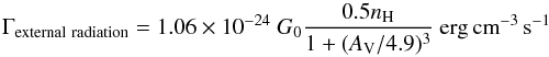 (1)where
AV is the local value of the attenuation from the surface
(which increases towards the centre from AV = 10 mag at the
outer boundary of the computational domain). We assume a standard external radiation field
and set G0 = 1. Compared to Lesaffre et al. (2005), we also slightly improve on the treatment of the dust
temperature by no longer assuming thermal equilibrium but computing the time evolution of
the dust temperature, including the thermal inertia of the grains. However, because this
inertia is very small, the results do not change, and the only noticeable effect of this
modification is to help improve the numerical convergence. The temperature of the gas itself
is controlled mainly by the balance between the grains heat exchange, the cosmic ray heating
and the CO cooling. The gas temperature does not always follow the grain temperature,
especially when the density is still low. This will be illustrated and discussed in
Sect. 5.2.
(1)where
AV is the local value of the attenuation from the surface
(which increases towards the centre from AV = 10 mag at the
outer boundary of the computational domain). We assume a standard external radiation field
and set G0 = 1. Compared to Lesaffre et al. (2005), we also slightly improve on the treatment of the dust
temperature by no longer assuming thermal equilibrium but computing the time evolution of
the dust temperature, including the thermal inertia of the grains. However, because this
inertia is very small, the results do not change, and the only noticeable effect of this
modification is to help improve the numerical convergence. The temperature of the gas itself
is controlled mainly by the balance between the grains heat exchange, the cosmic ray heating
and the CO cooling. The gas temperature does not always follow the grain temperature,
especially when the density is still low. This will be illustrated and discussed in
Sect. 5.2.
4. The importance of the ortho-H2 abundance at collapse start
Some chemical paths are sensitive to the presence of ortho-H2. It is true for
the first steps in ammonia formation (Le Bourlot
1991), and it is true for the first steps in the deuterium chemistry as first
discussed by Pineau des Forêts et al. (1991) and
Pagani et al. (1992), and further developed by
Walmsley et al. (2004), Flower et al. (2006b), and P09. It plays, however, no role in the warm
deuterium chemistry (based on CH ),
which has been observed by Parise et al. (2009). The
decay of ortho-H2 is a slow process, because of its presumably large initial
abundance. It is therefore the limiting factor in the deuteration process, in other words,
the one that gives the age of the core. We showed in P09 that its abundance has to drop
below ~1% of that of para-H2 to allow for large deuterium enrichments and the
time it took to decay to that level was compatible with the free-fall time. However, the
core probably does not start to form as soon as all atomic hydrogen has been converted to
molecular hydrogen, i.e., as soon as the molecular cloud is considered to be formed. Even if
molecular hydrogen has been produced with the largest possible OPR, namely 3, the question
arises whether in the cloud, the time has been long enough to significantly let
ortho-H2 decay before the prestellar core starts to form. Here we discuss the
initial OPR when H2 is formed on the grains and its decrease with time in the
cloud prior to the core contraction.
),
which has been observed by Parise et al. (2009). The
decay of ortho-H2 is a slow process, because of its presumably large initial
abundance. It is therefore the limiting factor in the deuteration process, in other words,
the one that gives the age of the core. We showed in P09 that its abundance has to drop
below ~1% of that of para-H2 to allow for large deuterium enrichments and the
time it took to decay to that level was compatible with the free-fall time. However, the
core probably does not start to form as soon as all atomic hydrogen has been converted to
molecular hydrogen, i.e., as soon as the molecular cloud is considered to be formed. Even if
molecular hydrogen has been produced with the largest possible OPR, namely 3, the question
arises whether in the cloud, the time has been long enough to significantly let
ortho-H2 decay before the prestellar core starts to form. Here we discuss the
initial OPR when H2 is formed on the grains and its decrease with time in the
cloud prior to the core contraction.
4.1. The initial ortho-para H2 ratio at formation time
The 4.5 eV energy release of the H2 formation reaction is large enough to
populate many levels of both ortho and para species: it is hence generally accepted,
though not totally certain, that the OPR is 3:1 when H2 forms on grains. A
first laboratory confirmation has recently been brought by the experiment of Watanabe et al. (2010) conducted on amorphous solid
water. The ortho-para conversion of H2 can then occur in the gas phase and onto
the surface of dust grains (Le Bourlot 2000). The
conversion rate on a solid surface is, however, highly uncertain (Watanabe et al. 2010; Chehrouri et al.
2011). Once released in the gas phase, H2 tends to relax towards its
thermal equilibrium state but never reaches it because at trace abundance levels,
ortho-H2 destruction is compensated by fresh H2 formed onto grains
from residual H and from destruction of ions, such as
and
H2D+, which can release an ortho-H2 (Le Bourlot 1991; Flower
et al. 2006b). This equilibrium value is three to four orders of magnitude
greater than the thermal equilibrium value at 10 K (10-3 – a few
10-5 compared to 10-7, Flower
et al. 2006b; P09; Parise et al. 2011). It
is thus necessary to model the chemical evolution of the H2 OPR to understand
the evolution of dark clouds. We therefore adopt an H2 OPR of three at the
formation time of the molecule and now discuss the conversion processes in the gas phase
prior to the collapse start.
4.2. The new H2 + H+ reaction rate
Radiative transitions between the ortho and para forms of H2 are known to be
very slow, with an interconversion lifetime greater than the age of the Universe for the
J = 1–0 transition (Pachucki &
Komasa 2008). Inelastic collisions are unable to change the spin state of
H2 either. Therefore only reactions with cations, mostly H+ and
, can perform such
an exchange. The H2 + reaction rate
has been statistically estimated by Hugo et al.
(2009), and recently, we performed an accurate, fully quantum calculation of the
H2 + H+ reaction rate (Honvault
et al. 2011a,b, 2012). The Kooij/Arrhenius rate formula for the
ortho-H2(J = 1) + H+ →
para-H2(J = 0) + H+ reaction is
 cm3 s-1
(from Honvault et al. 2011b)1. At 10 K, the new rate for this reaction is 62% lower than the one
previously estimated by Gerlich (1990),
1.13 × 10⁻¹⁰ and 2.972 × 10⁻¹⁰ cm3 s-1,
but it is 43% lower than the one used even at 10 K in Le
Bourlot (1991), Walmsley et al. (2004),
Flower et al. (2006b), and P09; i.e., 2
× 10-10 cm3 s-1, which is the rate value that was
only valid above 20 K in Gerlich (1990) Eq. (10).
Both the H2 + and the
H2 + H+ reactions have rates an order of magnitude lower than the
Langevin rate. As we show below, in the depleted core, H+ can become the
dominant cation and rule the decay of ortho-H2.
cm3 s-1
(from Honvault et al. 2011b)1. At 10 K, the new rate for this reaction is 62% lower than the one
previously estimated by Gerlich (1990),
1.13 × 10⁻¹⁰ and 2.972 × 10⁻¹⁰ cm3 s-1,
but it is 43% lower than the one used even at 10 K in Le
Bourlot (1991), Walmsley et al. (2004),
Flower et al. (2006b), and P09; i.e., 2
× 10-10 cm3 s-1, which is the rate value that was
only valid above 20 K in Gerlich (1990) Eq. (10).
Both the H2 + and the
H2 + H+ reactions have rates an order of magnitude lower than the
Langevin rate. As we show below, in the depleted core, H+ can become the
dominant cation and rule the decay of ortho-H2.
4.3. The evolution of the H2 OPR in the undepleted and low-density phase of dark clouds
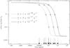 |
Fig. 1 Ortho-H2 abundance variation with time for 3 different values of ζ, the cosmic ray ionization rate. Crosses and arrows indicate the time it takes to reach an OPR of 1 (full arrows), 0.1 (dashed arrows), and 0.01 (dotted arrows) for a starting value of 3. The calculations are done for a temperature of 10 K and a density of n(H + 2H2) = 2 × 104 cm-3. |
Though the timescale for converting the bulk of atomic hydrogen to molecular hydrogen is
still a debated question, we can conventionally set the birth of the molecular cloud at
the time when this conversion is almost complete. From that moment, ortho-H2 is
slowly changing to para-H2, and the question arises as to how long this takes.
To address this question, we merged one of the recent Ohio State University (OSU) reaction
files available (osu_01_2009) with our own deuterium chemistry reaction file and ran the
new file with our modified version of Nahoon (for the original version, see Wakelam et al. 2005), as described in P09, to introduce
the ortho and para states of H2, and their
related isotopologues and ions (H ,
D2, etc.). All important reactions involving H2 or
as reactants in the
OSU file have been adapted to the ortho and para states of these species, but minor
reactions producing H2, such as CH+ + NH2 →
HCN+ + H2, have only been considered to produce
para-H2, which is the most energetically favourable case. We checked that this
approximation is not too strong and found that, after 105 years of model
evolution for example, 99.9% of the production reactions of para-H2 are due to
reactions of ortho-H2 with H+ and
. We ran the model
for a cloud with a density of n(H + 2H2) = 2
× 104 cm-3, 10 K, grain radius of 0.1 μm, and
the standard cosmic ray ionization rate, ζ of
1 × 10-17 s-1, which is in fact near the lower end of the range
of estimated values in the literature (Padovani et al.
2009). We tried different C/O ratios from 0.4 to 1 and, as expected, found no
major difference for the evolution of the H+ and
abundances and
therefore a similar decay rate of the H2 OPR, even though the main species that
react with these two cations are completely different whether the cloud is oxygen-rich or
carbon-rich. In this molecular-undepleted model, the recombination of H+ and
on negatively
charged grains remains a minor route to suppressing these cations, and therefore, grains
with larger size, as witnessed via the coreshine effect (Pagani et al. 2010b), have no influence on the result either. Higher cosmic ray
ionization rates have a predictable effect: they increase the production of H+
and and therefore
accelerate the decay of ortho-H2. Figure 1
shows the variation in ortho-H2 abundance with time for three different values
of ζ (1, 3, and 10 × 10-17 s-1). For the lowest
of the three, the OPR remains above one during one million years and drops below 1% in ten
million years. If we increase ζ by a factor of 10, the timescale also
drops by a factor of 10. In P09, only an initial OPR of 3 at the beginning of the
prestellar core phase was considered to model the production of deuterated species, and
the high OPR ratio was the limiting factor to the emergence of these species (see P09
their Fig. 8). Any lower OPR, either because H2 production on grains depart
from the statistical ratio or because the cloud is old enough for a given cosmic ray
ionization rate, would greatly accelerate the apparition of several deuterated species,
especially DCO+, and they would reach unobserved high abundances all over the
cloud, not only in the depleted cores (Pagani et al.
2011). OPR starting values below 0.1 are therefore excluded, and for values close
to 0.1, either clouds have a very short lifetime or the cosmic ray ionization rate is
lower than 1 × 10-17 s-1, which might be difficult to explain
(Padovani et al. 2009). It therefore seems most
probable that at the moment that dark clouds form and become molecular, the H2
OPR is between >0.1 and 3. In B68, Troscompt et al. (2009) constrain the H2 OPR below 1, from
H2CO anomalous absorption observations.
,
D2, etc.). All important reactions involving H2 or
as reactants in the
OSU file have been adapted to the ortho and para states of these species, but minor
reactions producing H2, such as CH+ + NH2 →
HCN+ + H2, have only been considered to produce
para-H2, which is the most energetically favourable case. We checked that this
approximation is not too strong and found that, after 105 years of model
evolution for example, 99.9% of the production reactions of para-H2 are due to
reactions of ortho-H2 with H+ and
. We ran the model
for a cloud with a density of n(H + 2H2) = 2
× 104 cm-3, 10 K, grain radius of 0.1 μm, and
the standard cosmic ray ionization rate, ζ of
1 × 10-17 s-1, which is in fact near the lower end of the range
of estimated values in the literature (Padovani et al.
2009). We tried different C/O ratios from 0.4 to 1 and, as expected, found no
major difference for the evolution of the H+ and
abundances and
therefore a similar decay rate of the H2 OPR, even though the main species that
react with these two cations are completely different whether the cloud is oxygen-rich or
carbon-rich. In this molecular-undepleted model, the recombination of H+ and
on negatively
charged grains remains a minor route to suppressing these cations, and therefore, grains
with larger size, as witnessed via the coreshine effect (Pagani et al. 2010b), have no influence on the result either. Higher cosmic ray
ionization rates have a predictable effect: they increase the production of H+
and and therefore
accelerate the decay of ortho-H2. Figure 1
shows the variation in ortho-H2 abundance with time for three different values
of ζ (1, 3, and 10 × 10-17 s-1). For the lowest
of the three, the OPR remains above one during one million years and drops below 1% in ten
million years. If we increase ζ by a factor of 10, the timescale also
drops by a factor of 10. In P09, only an initial OPR of 3 at the beginning of the
prestellar core phase was considered to model the production of deuterated species, and
the high OPR ratio was the limiting factor to the emergence of these species (see P09
their Fig. 8). Any lower OPR, either because H2 production on grains depart
from the statistical ratio or because the cloud is old enough for a given cosmic ray
ionization rate, would greatly accelerate the apparition of several deuterated species,
especially DCO+, and they would reach unobserved high abundances all over the
cloud, not only in the depleted cores (Pagani et al.
2011). OPR starting values below 0.1 are therefore excluded, and for values close
to 0.1, either clouds have a very short lifetime or the cosmic ray ionization rate is
lower than 1 × 10-17 s-1, which might be difficult to explain
(Padovani et al. 2009). It therefore seems most
probable that at the moment that dark clouds form and become molecular, the H2
OPR is between >0.1 and 3. In B68, Troscompt et al. (2009) constrain the H2 OPR below 1, from
H2CO anomalous absorption observations.
5. The model results
We present first the density profile evolution for both a fast and a slow collapse with average conditions. This sets up a frame with which we compare the N2D+/N2H+ ratio profile variation between the two types of models and subsequently the impact of the variations in different parameters on these profiles.
5.1. The density profile
The 1D model starts with a constant proton density set at 104 H cm-3, a (depleted) CO abundance of X[CO] = CO/H2 = 2 × 10⁻⁶, and a temperature of 10 K. All the hydrogen is molecular from the start, and therefore the initial proton density is equivalent to a particle density of 5900 (H2 + He) cm-3. We apply either a low external pressure (pext/kB = 2.8 × 10⁴ K cm-3, where kB is the Boltzmann constant), increasing slowly with a growth timescale of 107 years (see Lesaffre et al. 2005, Sect. 2.1) to induce a slow collapse, or an external pressure about three times higher (pext/kB = 8 × 10⁴ K cm-3) but constant in time to induce a fast collapse, but low enough to avoid a shock front. Depending on the parameters (e.g., the cooling of the cloud depends on the CO abundance), the fast collapse reaches a density of ~106 cm-3 in a few hundred thousand years, comparable to the free-fall time, while the slow collapse is typically ten times slower (Fig. 2), taking ~5 My to reach the same density. This timescale is comparable to the timescale predicted for models of prestellar core formation by ambipolar diffusion (Tassis & Mouschovias 2007). In the slow collapse model, we start with an external pressure slightly below the internal pressure of the cloud, estimated at thermal balance between heating and cooling, so, the cloud starts with a small expansion before contracting. In Fig. 2, we have selected three representative density profiles, which are quite similar for both models. The main difference is that during the first couple of million years, during the slow collapse, the cloud oscillates around a density of a few 104 cm-3 after the small expansion, before starting to contract quasi-statically. The first slow collapse profile is traced just after the end of the oscillation, which occurs ~1 My after the start of the model. At 700 yr, the profile is identical for both types of collapse and traces the initial state, i.e. 104 cm-3. Hereafter, we will call these models the fast model and the slow model. The time intervals to reach given central densities can change slightly between models when we vary the different input parameters to be tested, but the change is of the order of 15% maximum except when the heating or the cooling are modified (e.g. CO abundance variation, because CO is the main coolant of the cloud and therefore its presence helps accelerate the contraction, or ζ increase, which increases the heating input to the cloud), in which case we readjust the initial external pressure to return close to the 0.5 and 5 My duration of the models.
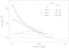 |
Fig. 2 Density profile evolution with a low, growing, external pressure (slow collapse, dashed lines) and with a high, constant, external pressure (fast collapse, full lines). The conditions after 700 yr of evolution are still identical and traced only once. The increasing ages follow the increasing central densities. |
 |
Fig. 3 Column density profile evolution with a low, growing, external pressure (slow collapse, dashed lines) and with a high, constant, external pressure (fast collapse, full lines). The conditions after 700 yr of evolution are still identical and traced only once. The increasing ages follow the increasing central column densities. |
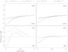 |
Fig. 4 Evolution of the dust (top row) and gas (bottom row) temperatures with time for the slow (right-hand side) and fast (left-hand side) models. The results are traced for the same density profiles as those in Fig. 2. The above-mentioned values indicate the peak central densities. |
5.2. Grain and gas temperatures
In the early phases, the gas thermal balance is dominated by CO cooling and photo-electric heating. The cosmic ray heating throughout the whole cloud amounts to a smaller contribution. On the other hand, the grain temperature is controlled by the radiative balance between the external radiative heating and the grain emissivity. Both temperatures (grain and gas) are then independent of each other. This remains true in the envelope throughout all runs. However, when the core is dense enough to be shielded from external photons, the grain heating becomes dominated by the collisional exchange with the gas and the compressional heating becomes the main source of heat for the gas. At that point, the compressional heating is transferred to the grains via collisions and is then evacuated by the radiation off the grains. As the density increases, the grain and gas temperatures become closer and closer to the cosmic microwave background radiation temperature (2.725 K). Figure 4 shows the evolution of the gas and dust temperatures during the contraction. The bump at radius 0.03 pc in the gas temperature profile of the first snapshot (dashed line, 2 × 104 cm-3 case) of the fast case is due to the compressional heating of a pressure wave which is still propagating inward at this time, while the density is still too low to couple the gas and the dust efficiently. Owing to the spherical convergence towards the centre, this bump later steepens to reach 23 K at its maximum when it hits the centre. However, this temperature rise lasts only for a short time (the central region, <0.01 pc, remains above 15 K for 4 × 10⁴ years only) and is not seen to significantly affect the chemical composition of the gas. The pressure wave dies out shortly after it moves back outwards. When the CO depletion is treated self-consistently, the pressure bump effect is even more attenuated, because the enhanced CO cooling forces temperature to a lower level as the pressure wave passes before CO becomes strongly depleted. No surge is seen in the slow case.
5.3. Model predictions
We first compare the deuteration profile for the slow and fast models in between them, and then present their sensitivity to different parameters for each of them separately by comparison with the first two (fast and slow) models taken as references.
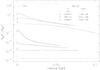 |
Fig. 5 Evolution of the N2D+/N2H+ ratio with time for the slow (dashed lines) and fast (full lines) models. The dotted line traces the slow/fast ratio for the last epoch (corresponding to a peak density of 2 × 106 cm-3). The results are traced for the same density profiles as those in Fig. 2. |
5.3.1. The reference models
Figure 5 shows the N2D+/N2H+ ratio for both models with X[CO] = 2 × 10⁻⁶ (equivalent to a depletion factor between 50 and 100 for a standard undepleted CO abundance between 1 and 2 × 10⁻⁴, Dickman 1978; Pineda et al. 2010. This value is close to typical depletion values found in the literature, such as in Tafalla et al. 2002 or Pagani et al. 2005), X[N2] = 3 × 10⁻⁷, both uniform and constant from the start (this value is representative of the values we found in P09. As its abundance plays a negligible role in the model, N2 will always be kept constant and uniform), a grain radius of 0.1 μm, an H2 OPR of 3, and a cosmic ray ionization rate of 1 × 10-17 s-1. The dust-to-gas mass ratio is 0.01 and the dust density is 3 g cm-3, the values usually adopted in chemical models. There is a large difference between the two models. The slow model has reached steady state in the outer layers before the density profile has reached its 106 cm-3 peak density and the difference in the ratio profile between slow and fast models is variable, ranging from 70 to 200 for the final density profile. As expected the models can help to distinguish slow and fast collapse theories with an unambiguous N2D+/N2H+ ratio profile variation.
This pair of models will be the reference for further comparisons below. For each model, slow or fast, we compare the new model with the one presented here in the next figures (new model = full lines, reference model = dashed line except where stated differently). To keep the figures readable, we compare the fast and slow models separately but plot them next to each other on identical scales.
5.3.2. The temperature sensitivity
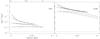 |
Fig. 6 Evolution of the N2D+/N2H+ ratio with temperature for the slow (right) and fast (left) models. In the reference model, the temperature of the chemical network is the temperature of the gas. The two other cases are for constant temperature imposed on the chemical network. To see the differences better, the reference model has been drawn with the full line mode (from respectively the slow and fast cases displayed in Fig. 5). |
During the contraction of the cloud, the gas and dust temperatures evolve as a result of imbalance between heating and cooling processes (see Sects. 3 and 5.2). The gas temperature influences those rates in the chemical network that are temperature dependent. Because the gas temperature profile that is self-consistently computed by the model differs from the gas temperature profile constrained by our N2H+ observations and radiative transfer modelling of L183 (Pagani et al. 2007, though L183 might not be a reference case in terms of the temperature profile by itself), we have tested what would happen if we kept the chemical network temperature constant at low values (between 7 K and 15 K). Figure 6 shows that the N2D+/N2H+ ratio is slightly flatter with fixed temperatures as a function of radius for the fast case, and for the slow case it is basically unchanged with a slightly different equilibrium value towards the centre, which can be linked to the final temperature (similar exemples are given in Parise et al. 2011). As we mention in Sect. 5.2, the pressure wave also has little effect on the chemistry, past the transient event in the fast case. Overall the variation is negligible, and the actual temperature profile is not a major source of uncertainty on the diazenylium deuteration enrichment estimate.
5.3.3. The CO abundance impact
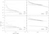 |
Fig. 7 Evolution of the N2D+/N2H+ ratio with time for the slow (right) and fast (left) models as a function of CO depletion (depletion multiplied by 2 in the top row, X[CO] = 1 × 10⁻⁶, divided by 5 in the bottom row, X[CO] = 1 × 10⁻⁵). The dashed lines trace the reference results (from respectively the slow and fast cases displayed in Fig. 5). The dotted line traces the new versus reference model ratio for the last epoch (corresponding to a peak density of 2 × 106 cm-3) in each frame. The results are traced for the same density profiles as those in Fig. 2. |
Constant CO abundance
The impact of CO abundance on the diazenylium ratio is displayed in Fig. 7. From the reference models, we have either
decreased the CO abundance (or increased the depletion) by a factor of 2
(X[CO] = 1 × 10⁻⁶, depletion factor between 100 and
200) or increased it by a factor of 5 (X[CO] = 1 × 10⁻⁵,
depletion factor between 10 and 20), to cover the usual range of local depletion
factors found in the literature (e.g. Caselli et al.
1999; Bergin et al. 2002; Bacmann et al. 2002; Tafalla et al. 2004; Pagani et al.
2005). The fast model gives a stronger deuteration level (gain ≈ 2–4) when
reaching the peak density if CO is depleted further or a much lower deuteration (drop
up to 30) if CO is less depleted. This is due to a higher fraction of
H2D+ being diverted to react with CO instead of HD (and
therefore a diminished production of the D2H+ and
deuteration vectors). The effect is therefore cumulative which explains the
amplification between the CO increase and the spectacular deuteration profile drop.
The slow model shows little sensitivity to the decrease in CO abundance but the factor
5 increase has a more dramatic effect. The final deuteration profile drops by up to a
factor of 8. This is one of the two cases where the
N2D+/N2H+ ratio remains below five in
the slow model, which could marginally fit some observations, especially if the peak
density is still low. However, the slow model leaves ample time for CO to deplete by
more than the factor 10–20 used here, and therefore this situation might be uncommon.
With a freeze-out timescale
τfo = 5 × 10⁹/nH2 years
(Bergin & Tafalla 2007), a depletion
factor of 20 is reached in 1.5 My for a density as low as
1 × 104 cm-3.
Dynamic CO depletion.
We now follow the dynamical depletion of CO during the contraction starting from a
CO/H2 relative abundance of 1 × 10⁻⁴ (Fig. 8). If the CO depletion mechanism is understood
relatively well, its desorption is much less certain (e.g. Öberg et al. 2005; Bisschop et al.
2006; Roberts et al. 2007; Öberg et al. 2009). Therefore it did not seem safe
to force desorption evolution on the model in this present study, especially since a
full model would need to include all species not depleted at the start with a large
chemical network to follow their overall disappearance along with CO in the
contracting and depleting core, which is beyond the scope of the present model. Even
limiting the depleting species to CO and N2 is a problem since their very
different depletion profile behaviour is not explained by recent models and laboratory
work, (see Öberg et al. 2005; Bisschop et al. 2006; Pagani et al. 2012a). However, the slow disappearance of CO must
slow the deuteration of N2H+ down, and we need to check the
importance of the effect to evaluate its impact on the model’s behaviour. We have
therefore added two rates in the chemical model, one to describe the sticking
probability of CO on the grains upon collision (which we set to 1, following the
laboratory work of Bisschop et al. 2006, which
gives a lower limit of 0.87 ± 0.05), and the other to describe the CO desorption upon
the cosmic ray impact on the dust grains. More details are given in Lesaffre et al. (2005, their Sect. 3.1.2). The CO
abundance evolution is displayed in the two upper boxes of Fig. 8. In the centre, the depletion can reach a factor of ~500 but in
the outer parts of the prestellar core, the depletion is less than a factor of 2.5 in
the fast case (after 0.5 My) and about a factor of 5 in the slow case (after a
few My). Such slopes are possibly seen in a few Taurus cases (Tafalla et al. 2002, 2004)
but do not seem to fit the model in B68 (Bergin et al.
2006), or the L1506C case (Pagani et al.
2010a), which shows a steep drop in CO abundance even for relatively low
density and extinction. Therefore this dynamical CO model may represent some real
cases but not all of them. Because CO is more abundant by more than an order of
magnitude in the outer parts compared to the reference model, its destruction of
and
H2D+ prevents an efficient deuteration of
N2H+. In the fast case, the deuteration is 2 to 14 times lower
for the final density profile. In the slow case, though the production of
D2H+ and are
slowed down by the higher CO abundance, these species eventually build up enough to
almost produce the same level of deuteration. For the final density profile, the
CO abundance is lower than in the reference case in the central 0.015 pc, and hence we
find a higher level of deuteration. The N2H+ and
N2D+ abundances are, however, somewhat reduced in the outer
parts of the core because of the higher abundance of CO (but since N2
chemistry is not dealt with, this has few implications).
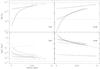 |
Fig. 8 Evolution of the N2D+/N2H+ ratio when CO depletion is varied compared to constant depletion, for the slow (right) and fast (left) models. CO variation is shown in the upper graphics, constant depleted CO appears as long dashed lines. In the bottom row, the dashed lines trace the reference results (from Fig. 5) and the dotted line traces the new versus reference model ratio for the last epoch (corresponding to a peak density of 2 × 106 cm-3) in each frame. |
5.3.4. The N2 abundance impact
As expected, we found no influence whatsoever on the diazenylium ratio when varying the N2 abundance from 1 × 10⁻⁹ to 5 × 10⁻⁷. The main impact is to change the diazenylium isotopologue abundances.
5.3.5. The H2 OPR impact
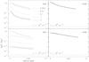 |
Fig. 9 Evolution of the N2D+/N2H+ ratio with the H2 OPR values at the beginning of core contraction for the slow (right) and fast (left) models. The bottom row corresponds to the density profile with peak density of 105 cm-3 and the top row to the profile with peak density of 2 × 106 cm-3 (from Fig. 2). Initial OPR values are listed in the top left image. The full lines (OPR = 3) also trace the reference results (from Fig. 5). |
The reference models both started with an H2 OPR of 3. Though we do not expect OPR ratios lower than ~0.1 typically at the start of the contraction (see Sect. 4.3), we have tested the effect of different initial OPR values from 1 down to 0.003 (Fig. 9). To avoid crowding in Fig. 9, we display only the two highest density profiles (peak densities of 105 and 106 cm-3) in two different frames for five OPR values (0.003, 0.01, 0.1, 1, and 3). The slow model is totally insensitive to initial OPR variations, which indicates that the cloud is old enough to have already converted most of its ortho-H2 to para-H2, bringing maximum deuteration capability even for high initial OPRs. The slow model is evolving with its chemistry in a steady-state situation before density becomes really high. For the fast model, the variation is more dramatic. For OPR ≤ 0.01, the model is close to chemical steady-state and hardly discernable from the slow model (observational uncertainties would be much larger than their differences). This is not surprising since the main slow evolving chemical species is the ortho-H2, everything else adjusting rapidly to its new value. Therefore if the model starts at such low OPRs, full deuteration is expected from the start as shown in P09 (and DCO+ would be detectable all over the cloud as discussed in Pagani et al. 2011).
5.3.6. The cosmic ray impact
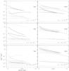 |
Fig. 10 Evolution of the N2D+/N2H+ ratio when the cosmic ray ionization rate is divided by 3 (bottom row), multiplied by 3 (middle row) and by 10 (top row) for the slow (right) and fast (left) models. The dotted line traces the new versus the reference model ratio for the last epoch (corresponding to a peak density of 2 × 106 cm-3) in each frame. The dashed lines trace the reference results (from Fig. 5). |
The cosmic ray ionization rate is not well known and seems to vary from place to place or from the diffuse medium to the dense medium (Padovani et al. 2009). As mentioned above (Sect. 4.3), a cosmic ray ionization rate below 1 × 10-17 s-1 seems improbable, and increasing the rate will accelerate the decay of ortho-H2. We tested one case with a lower rate though (3 × 10-18 s-1), and two cases with a higher rate (3 × 10-17 s-1 and 1 × 10-16 s-1, Fig. 10). Decreasing the rate slows down the chemistry because fewer ions are produced, while the chemistry is ion-driven. It is slowed so much that deuteration drops by a factor as high as 100. This is also the only situation for which the slow case does not reach equilibrium before the density has neared 1 × 105 cm-3. However, once the equilibrium has been reached, the deuteration of diazenylium is twice as high as in the standard case because of the lack of electrons to destroy the various deuterated ions. Increasing the cosmic ray ionization rate by as little as a factor of 3 has also a major impact on the chemical evolution of the cloud. The ortho-H2 abundance drops faster and the N2D+/N2H+ ratio increases faster for the fast model. The slow model is again evolving in steady-state mode, but the equilibrium settles lower than in the reference case. This is due to the higher electron abundance, directly proportional to the cosmic ray ionization rate, which increases the recombination efficiency of the cations and therefore prevents these cations from proceeding farther along the deuteration path. When increasing the cosmic ray ionization rate up to 1 × 10-16 s-1, the electron density increases further, so the deuterium profiles become even lower. In such cases, for moderate densities, the slow model deuteration level may become compatible with some observations.
5.3.7. The grain size impact
Grain size in dark clouds is an open subject that might improve with the combination of 3D radiative transfer dust models and diffraction observations from optical to mid-infrared (Steinacker et al. 2010; Pagani et al. 2010b; Juvela et al. 2012). A standard grain size of 0.1 μm is usually assumed in chemical models, but this is a strong approximation that might not be valid. In typical models, ~90% of the grains are negatively charged regardless of their size, and following Draine & Sutin (1987), the grains are in principle able to carry only one electron. Therefore the average size of the grains determines the density number of charged grains and their ability to neutralize H+ ions. For molecule-rich models (i.e. models without depletion), the recombination on grains is negligible, and the grain size does not matter. However, here recombination has a major impact, therefore the question is what size of grains should we use in prestellar cores. Following our recent coreshine results, 50% of a large sample of prestellar cores have large grains (Pagani et al. 2010b), but on the other hand, Ormel et al. (2009) show that the grain size distribution shows a double peak profile (before it reaches a steady state between coagulation and fragmentation), with one peak of growing size grains and one peak of constant small size grains of comparable importance. While the growing size grains fraction can explain the coreshine effect, the small size grains will maintain a large number of grains, hence of negatively charged grains. We have therefore explored the behaviour of our model with grains of 0.05 μm and 0.3 μm radius.
Increasing the grain size increases the abundance of H+, as less negatively charged grains are available for recombination with H+. In turn, the ortho-to-para H2 conversion efficiency increases and deuteration efficiency follows. Like in the previous case, the fast case deuteration efficiency is higher (Fig. 11). However, the lower density number of grains also absorb fewer electrons, and the number of free electrons remains higher, which brings us back to the previous situation, too. A higher cosmic ray ionization rate or bigger grains have the same kind of influence on the deuteration efficiency in depleted cores. If we decrease the grain size, smaller grains are more numerous, and will interact more often with H+ and the ortho-to-para H2 conversion efficiency will diminish. Opposite effects are seen as expected, however the effect is very weak.
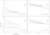 |
Fig. 11 Evolution of the N2D+/N2H+ ratio when the grain size is multiplied by 3 (bottom row) or divided by 2 (top row) for the slow (right) and fast (left) models. The dashed lines trace the reference results (from Fig. 5). The dotted line traces the new versus reference model ratio for the last epoch (corresponding to a peak density of 2 × 106 cm-3) in each frame. |
5.3.8. Slow versus fast models: a summary
Overall, the slow model has a relatively weak dependence upon all the possible initial conditions we have tested, while the fast model is sensitive to them but always remains distinct in its predictions from the slow model. Therefore, if the observations are found to fit one of these models best (without many possibilities of adjustment for the slow model, with some flexibility for the fast one), we will be able to tell whether the deuteration of N2H+ is compatible with rapid or slow collapse, independently of the initial conditions. Only two cases could prevent us from concluding: if the initial H2 OPR is already below 1–10% before the cloud starts to collapse, or, if the cosmic ray ionization rate is high. But that might have other consequences, which can be tested like the presence of DCO+ all over the cloud (Pagani et al. 2011).
For the sake of completeness, we also compared the deuteration evolution using the old ortho-to-para conversion rate from Gerlich (1990) to our new one (see Sect. 4.2). Overall, the deuteration efficiency has dropped by a factor of 3 with the new, slower rate in the fast model, while our new rate has no influence in the slow model case, as with most of the other parameters (see Appendix A).
6. The L183 case: discussion
We now compare these models to our L183 observations in the same manner as in P09 but with a 1D evolving model instead of a juxtaposition of layers of different and constant densities. We first searched the closest density profile (Fig. 12). The fit is not very good, which does not come as a surprise since the collapse model displays a density slope close to ρ ∝ r-2 from r = 0.003 pc (=600 AU) outward, while we showed that our data are compatible with ρ ∝ r-1 (Pagani et al. 2004) up to 0.02 pc = 4000 AU), a feature seemingly difficult to explain apart from some possible logotropic models (see Pagani et al. 2004, for a discussion). The three successive steps of the model calculations traced in Fig. 12 show that only the very inner part of the density profile keeps increasing after a while. It is therefore difficult to fit our observed density profile precisely, even allowing for a factor of 2 variation in the density values, and we decided to take the profile that best fits the inner density part of our data, i.e. to stop the model when its peak density reaches ~2 × 10⁶ H2 molecules cm-3. As discussed above (Sect. 5.1), the density profile remains basically the same in the density regime we are interested in here, whether coming from a slow collapse or from a fast collapse model.
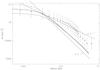 |
Fig. 12 Comparison between models and the L183 observed density profile (from Pagani et al. 2007). The error bar represents a variation by a factor of 2, not a real error estimate. The dashed, full, and dotted lines are the three successive steps from one of the models. The x axis is the cylindrical radius. |
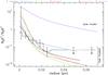 |
Fig. 13 Comparison between different models output for the peak density matching the observations and the N2D+/N2H+ local abundance ratio derived from the L183 observations (from Pagani et al. 2007). The error bars represent the maximum (resp. minimum) ratios using the maximum (resp. minimum) N2D+ abundance profile compared to the minimum (resp. maximum) N2H+ abundance profile as displayed in Fig. 4b of Pagani et al. (2007). The 7 models are listed in Table 1. The x axis is the cylindrical radius. |
Figure 13 shows the N2D+/N2H+ ratio for seven different models compared to the ratio derived from the analysis of the observations (Pagani et al. 2007). Table 1 indicates the main differences between the models. Only the fast collapse models can pretend to match the observations. If the fast model in the standard case (0.1 μm size grains, ζ = 1 × 10-17 s-1, fixed CO depletion by a factor of 50, H2 OPR = 3) does not produce enough deuteration (not shown here), small changes in one of the parameters can bring a reasonable fit to the observations. Either a 50% increase in the cosmic ionization rate (model 5), a stronger depletion by a factor of 4 (model 3), a grain size increase by a factor of 2 (model 1), or a slight deceleration of the contraction speed (model 4, collapse time increased by 30%) are enough to get a profile comparable to the observed one. A lower H2 OPR (0.5, model 6) similarly matches the observations. We tested the limits beyond which the model clearly does not fit the observations anymore and found that slowing down the collapse to make it last 0.8 My (collapse time increased by 60%) produces too much deuteration or that a starting H2 OPR of 0.2 was only marginally compatible with the observations. With ζ = 1 × 10-17 s-1, it takes about 3.5 My to go from an OPR of 3 to an OPR of 0.2. This sets an upper limit to the cloud age since its formation (which we define as the moment where most of atomic H is converted into H2) of ~4 My, i.e., a limit even lower than what we obtained from the absence of DCO+ outside prestellar cores in dark clouds (Pagani et al. 2011). Another interesting model is model 2, which combines both variable depletion profile and big grains, which could be closer to the actual situation than the other cases, though depletion is not yet measured precisely in the L183 core. Model 2 is the closest to the N2D+/N2H+ observed profile.
Because most slow models show little difference among them when reaching densities above 106 cm-3, we have shown only one typical case (model 7). Its predictions are far above the observations. In any case, it predicts an N2D+/N2H+ ratio above unity for most of the core and one order of magnitude too large at all radial distances. Therefore it seems impossible to adjust a slow-collapse model to our observations. This also excludes fast-collapse models for which the deuteration becomes too high, e.g. models where the initial H2 OPR ratio is already below 0.1, or with cosmic ray ionization rates too high.
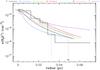 |
Fig. 14 Comparison between different models output for the peak density matching the observations and the H2D+ local density derived from the observations. The error bars represent the range of possible values fitting the observations (Fig. 3 of P09). The 7 models are listed in Table 1. |
The fit is also relatively good with ortho-H2D+ (Fig. 14). The average abundance is correct for the different
fast models and even for the slow model, but the profile is somewhat higher in the outer
parts than observed. The best model (model 2) for the
N2D+/N2H+ ratio is the worst one for the
abundance of H2D+. In the outer parts of the core, the models predict
too much H2D+. Despite this H2D+ abundance that
is too high beyond 0.03 pc, the Diazenylium fractionation remains slightly too low
(Fig. 13). This contradiction is only apparent
because the conversion of
to is lagging behind
since the density is too low in the outer part of the model, and the chemical model still
peaks on the production of H2D+ more than on its conversion
to D2H+ and . This species
(H2D+) is not the only deuteration partner of N2, and
therefore its abundance is not forcibly linked to the diazenylium fractionation (see
Sect. 3.3 in P09). This is why its similar abundance profile for the slow case is not linked
to the too high diazenylium deuteration profile of Fig. 13. Therefore the ortho-H2D+ abundance profile does not
distinguish between slow or fast models.
7. Conclusions
To observe the diazenylium fractionation profile across prestellar cores is a possible way to establish the ages of these cores. Deuteration enrichment is bound to increase in cold clouds, leading to a predictable diazenylium ratio profile. This should allow estimation of the ages of all prestellar cores that undergo CO depletion.
L183 is compatible with a fast collapse model starting with a high H2 OPR. An OPR ≥ 0.2 sets an upper limit to the beginning of the collapse of 3.5 My after the formation of the molecular cloud, and the fast collapse itself typically lasts 0.5 My (and ≤0.7 My). Therefore, the deuterated profile of diazenylium in L183 sets an upper limit of 4 My to the age of the core since the formation of the cloud. This result is not compatible with the slowest of the ambipolar diffusion-based contraction models and confirms the results found by Lee & Myers (1999). It also confirms that steady-state chemistry is not reached in prestellar cores and, in particular, in L183, so steady-state chemical models should be avoided at this stage of star formation.
Online material
Appendix A: The new H2 + H+ rate impact
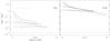 |
Fig. A.1 Evolution of the N2D+/N2H+ ratio with the old H2 + H+, for the slow (right) and fast (left) models. The dashed lines trace the reference results (from Fig. 5). The dotted line traces the new versus reference model ratio for the last epoch (corresponding to a peak density of 2 × 106 cm-3) in each frame. |
It is interesting to check the importance of the new ortho-to-para conversion rate of H2 on the deuteration efficiency because this conversion rate is the prime ruler among chemical reaction rates on the evolutionary time of the chemistry. Figure A.1 shows the deceleration of the deuteration with the new rate (which is the reference case, i.e. the dashed lines) compared to the old rate (Gerlich 1990, which is the test case here, i.e. the full lines). The difference in deuteration is a factor of 3 for the fast case. There is, however, almost no difference for the slow case, which has already reached steady state, even more so with the old, faster rate.
Appendix B: The D2H+/H2D+ ratio
We study in this appendix the sensitivity of the
para-D2H+/ortho-H2D+ (hereafter PDOH)
ratio to the different parameter variations we have studied in the main text. The
difficulty observing those lines from the ground makes them of limited interest as a
tool for studying cold cores, but they are nevertheless interesting values when such
observations have been achieved, because these are basically the only
isotopologues observable from the ground. Their ortho and para counterparts are above 1
THz and are difficult to detect due to the large energy difference between the upper and
ground levels, which is incompatible with the low temperature needed to have these
species produced in large quantities. Their detection in absorption would require a
strong background source, not available in all the presently known PSCs. Among the rare
detections, an interesting mapping of D2H+ has been reported by
Parise et al. (2011).
The parameters are varied in the same order as in Sect. 5 for the N2D+/N2H+ modelling.
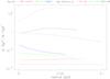 |
Fig. B.1 Evolution of the para-D2H+/ortho-H2D+ ratio with time for the slow (dashed lines) and fast (full lines) reference models. The dotted line traces the slow/fast ratio for the last epoch (corresponding to a peak density of 2 × 106 cm-3). The results are traced for the same density profiles as those in Fig. 2 |
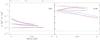 |
Fig. B.2 Evolution of the para-D2H+/ortho-H2D+ ratio with temperature for the slow (right) and fast (left) models. In the reference model, the temperature of the chemical network is the temperature of the gas. The two other cases are for constant temperature imposed on the chemical network. To better see the differences, the reference model has been drawn with the full line mode (from respectively the slow and fast cases displayed in Fig. B.1). The results are traced for the same density profiles as those in Fig. 2. |
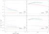 |
Fig. B.3 Evolution of the para-D2H+/ortho-H2D+ ratio with time for the slow (right) and fast (left) models as a function of CO depletion (depletion multiplied by 2 in the top row, divided by 5 in the bottom row). The dashed lines trace the reference results (from respectively the slow and fast cases displayed in Fig. B.1). The dotted line traces the new versus reference model ratio for the last epoch (corresponding to a peak density of 2 × 106 cm-3) in each frame. The results are traced for the same density profiles as those in Fig. 2. |
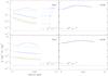 |
Fig. B.4 Evolution of the para-D2H+/ortho-H2D+ ratio with the H2 OPR for the slow (right) and fast (left) models. The bottom row corresponds to the density profile with peak density of 105 cm-3 and the top row to the profile with peak density of 2 × 106 cm-3 (from Fig. 2). OPR values are listed in the top left image. The dashed lines trace the reference results (from Fig. B.1). |
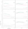 |
Fig. B.5 Evolution of the para-D2H+/ortho-H2D+ ratio when the cosmic ray ionization rate is multiplied by 3 (bottom row) and by 10 (top row) for the slow (right) and fast (left) models. The dotted line traces the new versus reference model ratio for the last epoch (corresponding to a peak density of 2 × 106 cm-3) in each frame. The dashed lines trace the reference results (from Fig. B.1). |
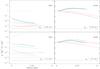 |
Fig. B.6 Evolution of the para-D2H+/ortho-H2D+ ratio when the grain size is multiplied by 3 (bottom row) or divided by 2 (top row) for the slow (right) and fast (left) models. The dashed lines trace the reference results (from Fig. B.1). The dotted line traces the new versus reference model ratio for the last epoch (corresponding to a peak density of 2 × 106 cm-3) in each frame. |
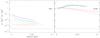 |
Fig. B.7 Evolution of the para-D2H+/ortho-H2D+ ratio with the old H2 + H+, for the slow (right) and fast (left) models. The dashed lines trace the reference results (from Fig. B.1). The dotted line traces the new versus reference model ratio for the last epoch (corresponding to a peak density of 2 × 106 cm-3) in each frame. |
Comments on the different figures.
Unlike the N2D+/N2H+ ratio evolution
with time, the PDOH ratio evolution is not forcibly monotonic because both species are
transient from to
, and the
two species are directly connected via chemical reactions (for
N2D+ and N2H+, this is true only for
reactions with H and D atoms, which play a minor role). Indeed, in the reference case
(Fig. B.1), this PDOH ratio first increases at
all radial distances in a similar manner and then, in the slow case, drops in the
inner 0.02 pc part with time. For the final density profile, the ratio is 5 to
300 times higher in the slow case than in the fast case. The latter has clearly not
reached steady state.
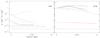 |
Fig. B.8 Evolution of the para-D2H+/ortho-H2D+ ratio when CO depletion is varying compared to constant depletion, for the slow (right) and fast (left) models. The dashed lines trace the reference results (from Fig. B.1) and the dotted line traces the new versus reference model ratio for the last epoch (corresponding to a peak density of 2 × 106 cm-3) in each frame. |
The sensitivity to temperature is slightly greater than for the N2D+/N2H+ ratio in the slow case (compare Figs. B.2a and 6) in a non-obvious fashion. The sensitivity to CO abundance follows expectations (Fig. B.3). When CO abundance increases, it reacts with a larger quantity of H2D+ ions, directly competing with HD to form HCO+ and DCO+ rather than D2H+. It is also visible in the slow process when the CO abundance is increased.
The initial OPR ratio at collapse start has the same influence on the PDOH ratio as on the N2D+/N2H+ ratio (Figs. B.4 vs. 9); i.e., as the initial OPR ratio is lowered, the chemistry approaches the steady state more and more. The slow case is already in steady-state and does not show any change at all.
Figure B.5 (cosmic ray ionization rate dependence) shows a strongly non-linear behaviour along the core radius and when the cosmic ray ionization rate is increased. In the fast collapse case, for ζ = 1 × 10-16 s-1, steady state is reached when arriving at the highest density after passing by a higher ratio value in the centre. The ratio has therefore not evolved monotonically.
For an average grain smaller than 0.1 μm, we find results similar to the N2D+/N2H+ ratio case (Figs. B.6 vs. 11), with a small decrease in the deuteration efficiency for the fast case and almost no change for the slow case. For large grains, the fast case shows a strong amplification, and for the slow case, the behaviour is non-linear, marking a small increase first and then a small decrease in the ratio.
The last two cases (sensitivity to the old H2 + H+ reaction rate, Fig. B.7, and to variable CO depletion, Fig. B.8) show the same behaviours as those reported for the N2D+/N2H+ ratio cases (Figs. A.1 and 8).
Overall, in the fast collapse case, the PDOH ratio remains almost always below 1 while it varies from 1 in the centre to ~5 at distances around 0.03–0.05 pc away from it for the slow case but some ambiguity can appear in several cases. In both the fast and the slow cases, the variation in the PDOH ratio can be non-monotonic and therefore not a good constraint to differentiate between the models.
Appendix C: Kooij/Arrhenius expression of the Hugo H + H2 isotopologues reaction rates and of the
H
isotopologues dissociative recombination rates2
+ H2 isotopologues reaction rates and of the
H
isotopologues dissociative recombination rates2
Hugo et al. (2009) fit their
+
H2 isotopologue reaction rate tables with the Arrhenius formula
(K = αe−β/T cm3 s-1).
However, they have validated their fits only in the 5–20 K temperature range. By
employing the more complete Kooij/Arrhenius formula
(K = α(T/300 K)βe−γ/T cm3 s-1)
and adjusting the coefficients by hand, we can provide a fit extending up to 50 K, the
maximum temperature given in Hugo et al. (2009)
tables, to a sufficient precision (<±10%). To compute the
Kooij/Arrhenius coefficients, we loaded the tabulated values (between 5 and 50 K), and
fitted the first two terms of the formula (α,β) by eye after
multiplying the rate by
eγ/T for the endothermic
reactions. We minimized the errors to keep them to a few % only over all the temperature
range. Figures C.1–C.3 show two examples of a fit. Figures C.1–C.2 show the fitting of an
endothermic reaction. At very low temperatures, the endothermic reaction coefficients
become low enough to drop below 10-20 and are zeroed in Hugo et al. (2009) reaction files. These values therefore remain
zeroed when corrected for the endothermicity (Fig. C.1) and cannot be recovered and used for the fit. The fit extrapolation is,
however, good enough, and its possible error is largely attenuated by the strong
endothermic correction (Fig. C.2), which makes the
rate drop quickly. In some cases, the Kooij formula cannot fit the data. Figure C.3 shows such a case for an exothermic reaction. The
fit is minimized so that the maximum error is the same in the middle and at the two ends
of the slope. The error remains lower than ±10% for all rates within the 5–50 K range
compared to the tabulated values. The Kooij/Arrhenius coefficients are given in
Table C.1.
In Table C.2, we present the Kooij/Arrhenius
coefficients of the dissociative recombination rates of the
isotopologues from P09.
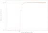 |
Fig. C.1 Fit for the reaction m- |
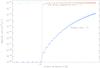 |
Fig. C.2 Same as Fig. C.1 but with a different Y-scale. The original rate is plotted in dark blue and the fit in cyan is the green fit equation with the endothermic correction (e−206/Tkin) reintroduced. The fit is good even for the departing first non-zeroed rates at low Tkin. |
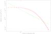 |
Fig. C.3 Fit for the reaction o-D2H+ + HD →
o- |
Kooij/Arrhenius coefficients of the +
H2 isotopologues reactions.
continued.
Kooij/Arrhenius coefficients of the dissociative recombination rates of the
isotopologues from P09.
Note the erratum: the constant coefficient is 1.82 × 10⁻¹⁰ cm-3 instead of 6.51 × 10⁻¹⁰ cm-3 (Honvault et al. 2012).
If authors want to use these parameterized rates, they should still quote the original works by Hugo et al. (2009) and P09 for the two sets, respectively.
Acknowledgments
T.G.L. would like to thank the Spanish Ministry of Science and Innovation for support under grants FIS2010-18132, FIS2011-29596-C02-01 and Consolider Ingenio 2010 CSD2009-00038. P.L. acknowledges support from the French embassy in the UK when he worked as overseas fellow at Churchill college, Cambridge, when this work was initiated in 2009. We thank the referee, B. Parise for a careful reading of the manuscript and many constructive criticisms and discussions that helped to improve the paper.
References
- Bacmann, A., Lefloch, B., Ceccarelli, C., et al. 2002, A&A, 389, L6 [NASA ADS] [CrossRef] [EDP Sciences] [Google Scholar]
- Bell, T. A., Willacy, K., Phillips, T. G., Allen, M., & Lis, D. C. 2011, ApJ, 731, 48 [NASA ADS] [CrossRef] [Google Scholar]
- Bergin, E. A., & Tafalla, M. 2007, ARA&A, 45, 339 [NASA ADS] [CrossRef] [Google Scholar]
- Bergin, E. A., Alves, J., Huard, T., & Lada, C. J. 2002, ApJ, 570, L101 [NASA ADS] [CrossRef] [Google Scholar]
- Bergin, E. A., Maret, S., Tak, F. F. S. V. D., et al. 2006, ApJ, 645, 369 [NASA ADS] [CrossRef] [MathSciNet] [Google Scholar]
- Bisschop, S. E., Fraser, H. J., Öberg, K. I., van Dishoeck, E. F., & Schlemmer, S. 2006, A&A, 449, 1297 [NASA ADS] [CrossRef] [EDP Sciences] [Google Scholar]
- Caselli, P. 2002, Planet. Space Sci., 50, 1133 [NASA ADS] [CrossRef] [Google Scholar]
- Caselli, P., Walmsley, C. M., Tafalla, M., Dore, L., & Myers, P. C. 1999, ApJ, 523, L165 [NASA ADS] [CrossRef] [Google Scholar]
- Caselli, P., van der Tak, F. F. S., Ceccarelli, C., & Bacmann, A. 2003, A&A, 403, L37 [NASA ADS] [CrossRef] [EDP Sciences] [Google Scholar]
- Caselli, P., Vastel, C., Ceccarelli, C., et al. 2008, A&A, 492, 703 [NASA ADS] [CrossRef] [EDP Sciences] [Google Scholar]
- Chehrouri, M., Fillion, J., Chaabouni, H., et al. 2011, Phys. Chem. Chem. Phys. (Incorporating Faraday Transactions), 13, 2172 [NASA ADS] [CrossRef] [Google Scholar]
- Crutcher, R. M., Wandelt, B., Heiles, C., Falgarone, E., & Troland, T. H. 2010, ApJ, 725, 466 [NASA ADS] [CrossRef] [Google Scholar]
- Dickman, R. L. 1978, ApJS, 37, 407 [NASA ADS] [CrossRef] [Google Scholar]
- Draine, B. T., & Sutin, B. 1987, ApJ, 320, 803 [NASA ADS] [CrossRef] [Google Scholar]
- Flower, D., Forêts, G. P. D., & Walmsley, M. 2004, A&A, 427, 887 [NASA ADS] [CrossRef] [EDP Sciences] [Google Scholar]
- Flower, D., Forêts, G. P. D., & Walmsley, M. 2006a, A&A, 456, 215 [NASA ADS] [CrossRef] [EDP Sciences] [Google Scholar]
- Flower, D., Forêts, G. P. D., & Walmsley, M. 2006b, A&A, 449, 621 [NASA ADS] [CrossRef] [EDP Sciences] [Google Scholar]
- Ford, A. B., & Shirley, Y. L. 2011, ApJ, 728, 144 [NASA ADS] [CrossRef] [Google Scholar]
- Gerlich, D. 1990, JCP, 92, 2377 [Google Scholar]
- Honvault, P., Jorfi, M., González-Lezana, T., Faure, A., & Pagani, L. 2011a, Phys. Rev. Lett., 107, 023201 [NASA ADS] [CrossRef] [Google Scholar]
- Honvault, P., Jorfi, M., González-Lezana, T., Faure, A., & Pagani, L. 2011b, Phys. Chem. Chem. Phys., 131, 19089 [CrossRef] [Google Scholar]
- Honvault, P., Jorfi, M., González-Lezana, T., Faure, A., & Pagani, L. 2012, Phys. Rev. Lett., 108, 109903 [NASA ADS] [CrossRef] [Google Scholar]
- Hugo, E., Asvany, O., & Schlemmer, S. 2009, JCP, 130, 164302 [Google Scholar]
- Juvela, M., Pelkonen, V.-M., White, G. J., et al. 2012, A&A, 544, A14 [NASA ADS] [CrossRef] [EDP Sciences] [Google Scholar]
- Le Bourlot, J. 1991, A&A, 242, 235 [NASA ADS] [Google Scholar]
- Le Bourlot, J. 2000, A&A, 360, 656 [Google Scholar]
- Lee, C. W., & Myers, P. C. 1999, ApJS, 123, 233 [NASA ADS] [CrossRef] [Google Scholar]
- Lesaffre, P., Belloche, A., Chièze, J.-P., & André, P. 2005, A&A, 443, 961 [NASA ADS] [CrossRef] [EDP Sciences] [Google Scholar]
- Lis, D. C., Roueff, E., Gerin, M., et al. 2002, ApJ, 571, L55 [NASA ADS] [CrossRef] [Google Scholar]
- Liszt, H. S. 2009, A&A, 508, 783 [NASA ADS] [CrossRef] [EDP Sciences] [Google Scholar]
- Nilsson, A., Hjalmarson, Å., Bergman, P., & Millar, T. J. 2000, A&A, 358, 257 [NASA ADS] [Google Scholar]
- Öberg, K. I., van Broekhuizen, F., Fraser, H. J., et al. 2005, ApJ, 621, L33 [NASA ADS] [CrossRef] [Google Scholar]
- Öberg, K. I., van Dishoeck, E. F., & Linnartz, H. 2009, A&A, 496, 281 [NASA ADS] [CrossRef] [EDP Sciences] [Google Scholar]
- Ormel, C. W., Paszun, D., Dominik, C., & Tielens, A. G. G. M. 2009, A&A, 502, 845 [NASA ADS] [CrossRef] [EDP Sciences] [Google Scholar]
- Pachucki, K., & Komasa, J. 2008, Phys. Rev. A, 77, 030501 [NASA ADS] [CrossRef] [Google Scholar]
- Padovani, M., Galli, D., & Glassgold, A. E. 2009, A&A, 501, 619 [NASA ADS] [CrossRef] [EDP Sciences] [Google Scholar]
- Pagani, L., Salez, M., & Wannier, P. G. 1992, A&A, 258, 479 [NASA ADS] [Google Scholar]
- Pagani, L., Bacmann, A., Motte, F., et al. 2004, A&A, 417, 605 [NASA ADS] [CrossRef] [EDP Sciences] [Google Scholar]
- Pagani, L., Pardo, J.-R., Apponi, A. J., Bacmann, A., & Cabrit, S. 2005, A&A, 429, 181 [NASA ADS] [CrossRef] [EDP Sciences] [Google Scholar]
- Pagani, L., Bacmann, A., Cabrit, S., & Vastel, C. 2007, A&A, 467, 179 [NASA ADS] [CrossRef] [EDP Sciences] [Google Scholar]
- Pagani, L., Vastel, C., Hugo, E., et al. 2009, A&A, 494, 623 (P09) [NASA ADS] [CrossRef] [EDP Sciences] [Google Scholar]
- Pagani, L., Ristorcelli, I., Boudet, N., et al. 2010a, A&A, 512, A3 [Google Scholar]
- Pagani, L., Steinacker, J., Bacmann, A., Stutz, A. M., & Henning, T. 2010b, Science, 329, 1622 [NASA ADS] [CrossRef] [PubMed] [Google Scholar]
- Pagani, L., Roueff, E., & Lesaffre, P. 2011, ApJ, 739, L35 [NASA ADS] [CrossRef] [Google Scholar]
- Pagani, L., Bourgoin, A., & Lique, F. 2012a, A&A, 548, L4 [CrossRef] [EDP Sciences] [Google Scholar]
- Pagani, L., Lefèvre, C., Bacmann, A., & Steinacker, J. 2012b, A&A, 541, A154 [NASA ADS] [CrossRef] [EDP Sciences] [Google Scholar]
- Parise, B., Castets, A., Herbst, E., et al. 2004, A&A, 416, 159 [NASA ADS] [CrossRef] [EDP Sciences] [Google Scholar]
- Parise, B., Leurini, S., Schilke, P., et al. 2009, A&A, 508, 737 [NASA ADS] [CrossRef] [EDP Sciences] [Google Scholar]
- Parise, B., Belloche, A., Du, F., Güsten, R., & Menten, K. M. 2011, A&A, 526, A31 [NASA ADS] [CrossRef] [EDP Sciences] [Google Scholar]
- Pineau des Forêts, G., Flower, D. R., & McCarroll, R. 1991, MNRAS, 248, 173 [NASA ADS] [Google Scholar]
- Pineda, J. L., Goldsmith, P. F., Chapman, N., et al. 2010, ApJ, 721, 686 [NASA ADS] [CrossRef] [Google Scholar]
- Roberts, H., Herbst, E., & Millar, T. J. 2004, A&A, 424, 905 [NASA ADS] [CrossRef] [EDP Sciences] [Google Scholar]
- Roberts, J. F., Rawlings, J. M. C., Viti, S., & Williams, D. A. 2007, MNRAS, 382, 733 [NASA ADS] [CrossRef] [Google Scholar]
- Sipilä, O., Hugo, E., Harju, J., et al. 2010, A&A, 509, A98 [NASA ADS] [CrossRef] [EDP Sciences] [Google Scholar]
- Steinacker, J., Pagani, L., Bacmann, A., & Guieu, S. 2010, A&A, 511, A9 [NASA ADS] [CrossRef] [EDP Sciences] [Google Scholar]
- Tafalla, M., Myers, P. C., Caselli, P., Walmsley, M., & Comito, C. 2002, ApJ, 569, 815 [NASA ADS] [CrossRef] [Google Scholar]
- Tafalla, M., Myers, P. C., Caselli, P., & Walmsley, M. 2004, A&A, 416, 191 [NASA ADS] [CrossRef] [EDP Sciences] [Google Scholar]
- Tak, F. F. S. V. D., Schilke, P., Müller, H. S. P., et al. 2002, A&A, 388, L53 [NASA ADS] [CrossRef] [EDP Sciences] [Google Scholar]
- Tassis, K., & Mouschovias, T. C. 2007, ApJ, 660, 388 [NASA ADS] [CrossRef] [Google Scholar]
- Troscompt, N., Faure, A., Maret, S., et al. 2009, A&A, 506, 1243 [NASA ADS] [CrossRef] [EDP Sciences] [Google Scholar]
- van Weeren, R. J., Brinch, C., & Hogerheijde, M. R. 2009, A&A, 497, 773 [NASA ADS] [CrossRef] [EDP Sciences] [Google Scholar]
- Vastel, C., Phillips, T. G., Caselli, P., Ceccarelli, C., & Pagani, L. 2006, Roy. Soc. London Philos. Trans. Ser. A, 364, 3081 [Google Scholar]
- Vastel, C., Phillips, T. G., & Yoshida, H. 2004, ApJ, 606, L127 [NASA ADS] [CrossRef] [Google Scholar]
- Wakelam, V., Selsis, F., Herbst, E., & Caselli, P. 2005, A&A, 444, 883 [NASA ADS] [CrossRef] [EDP Sciences] [Google Scholar]
- Walmsley, M., Flower, D., & Forêts, G. P. D. 2004, A&A, 418, 1035 [NASA ADS] [CrossRef] [EDP Sciences] [Google Scholar]
- Watanabe, N., Kimura, Y., Kouchi, A., et al. 2010, ApJ, 714, L233 [NASA ADS] [CrossRef] [Google Scholar]
- Zucconi, A., Walmsley, M., & Galli, D. 2001, A&A, 376, 650 [NASA ADS] [CrossRef] [EDP Sciences] [Google Scholar]
All Tables
Kooij/Arrhenius coefficients of the dissociative recombination rates of the
isotopologues from P09.
All Figures
|
Fig. 1 Ortho-H2 abundance variation with time for 3 different values of ζ, the cosmic ray ionization rate. Crosses and arrows indicate the time it takes to reach an OPR of 1 (full arrows), 0.1 (dashed arrows), and 0.01 (dotted arrows) for a starting value of 3. The calculations are done for a temperature of 10 K and a density of n(H + 2H2) = 2 × 104 cm-3. |
| In the text | |
|
Fig. 2 Density profile evolution with a low, growing, external pressure (slow collapse, dashed lines) and with a high, constant, external pressure (fast collapse, full lines). The conditions after 700 yr of evolution are still identical and traced only once. The increasing ages follow the increasing central densities. |
| In the text | |
|
Fig. 3 Column density profile evolution with a low, growing, external pressure (slow collapse, dashed lines) and with a high, constant, external pressure (fast collapse, full lines). The conditions after 700 yr of evolution are still identical and traced only once. The increasing ages follow the increasing central column densities. |
| In the text | |
|
Fig. 4 Evolution of the dust (top row) and gas (bottom row) temperatures with time for the slow (right-hand side) and fast (left-hand side) models. The results are traced for the same density profiles as those in Fig. 2. The above-mentioned values indicate the peak central densities. |
| In the text | |
|
Fig. 5 Evolution of the N2D+/N2H+ ratio with time for the slow (dashed lines) and fast (full lines) models. The dotted line traces the slow/fast ratio for the last epoch (corresponding to a peak density of 2 × 106 cm-3). The results are traced for the same density profiles as those in Fig. 2. |
| In the text | |
|
Fig. 6 Evolution of the N2D+/N2H+ ratio with temperature for the slow (right) and fast (left) models. In the reference model, the temperature of the chemical network is the temperature of the gas. The two other cases are for constant temperature imposed on the chemical network. To see the differences better, the reference model has been drawn with the full line mode (from respectively the slow and fast cases displayed in Fig. 5). |
| In the text | |
|
Fig. 7 Evolution of the N2D+/N2H+ ratio with time for the slow (right) and fast (left) models as a function of CO depletion (depletion multiplied by 2 in the top row, X[CO] = 1 × 10⁻⁶, divided by 5 in the bottom row, X[CO] = 1 × 10⁻⁵). The dashed lines trace the reference results (from respectively the slow and fast cases displayed in Fig. 5). The dotted line traces the new versus reference model ratio for the last epoch (corresponding to a peak density of 2 × 106 cm-3) in each frame. The results are traced for the same density profiles as those in Fig. 2. |
| In the text | |
|
Fig. 8 Evolution of the N2D+/N2H+ ratio when CO depletion is varied compared to constant depletion, for the slow (right) and fast (left) models. CO variation is shown in the upper graphics, constant depleted CO appears as long dashed lines. In the bottom row, the dashed lines trace the reference results (from Fig. 5) and the dotted line traces the new versus reference model ratio for the last epoch (corresponding to a peak density of 2 × 106 cm-3) in each frame. |
| In the text | |
|
Fig. 9 Evolution of the N2D+/N2H+ ratio with the H2 OPR values at the beginning of core contraction for the slow (right) and fast (left) models. The bottom row corresponds to the density profile with peak density of 105 cm-3 and the top row to the profile with peak density of 2 × 106 cm-3 (from Fig. 2). Initial OPR values are listed in the top left image. The full lines (OPR = 3) also trace the reference results (from Fig. 5). |
| In the text | |
|
Fig. 10 Evolution of the N2D+/N2H+ ratio when the cosmic ray ionization rate is divided by 3 (bottom row), multiplied by 3 (middle row) and by 10 (top row) for the slow (right) and fast (left) models. The dotted line traces the new versus the reference model ratio for the last epoch (corresponding to a peak density of 2 × 106 cm-3) in each frame. The dashed lines trace the reference results (from Fig. 5). |
| In the text | |
|
Fig. 11 Evolution of the N2D+/N2H+ ratio when the grain size is multiplied by 3 (bottom row) or divided by 2 (top row) for the slow (right) and fast (left) models. The dashed lines trace the reference results (from Fig. 5). The dotted line traces the new versus reference model ratio for the last epoch (corresponding to a peak density of 2 × 106 cm-3) in each frame. |
| In the text | |
|
Fig. 12 Comparison between models and the L183 observed density profile (from Pagani et al. 2007). The error bar represents a variation by a factor of 2, not a real error estimate. The dashed, full, and dotted lines are the three successive steps from one of the models. The x axis is the cylindrical radius. |
| In the text | |
|
Fig. 13 Comparison between different models output for the peak density matching the observations and the N2D+/N2H+ local abundance ratio derived from the L183 observations (from Pagani et al. 2007). The error bars represent the maximum (resp. minimum) ratios using the maximum (resp. minimum) N2D+ abundance profile compared to the minimum (resp. maximum) N2H+ abundance profile as displayed in Fig. 4b of Pagani et al. (2007). The 7 models are listed in Table 1. The x axis is the cylindrical radius. |
| In the text | |
|
Fig. 14 Comparison between different models output for the peak density matching the observations and the H2D+ local density derived from the observations. The error bars represent the range of possible values fitting the observations (Fig. 3 of P09). The 7 models are listed in Table 1. |
| In the text | |
|
Fig. A.1 Evolution of the N2D+/N2H+ ratio with the old H2 + H+, for the slow (right) and fast (left) models. The dashed lines trace the reference results (from Fig. 5). The dotted line traces the new versus reference model ratio for the last epoch (corresponding to a peak density of 2 × 106 cm-3) in each frame. |
| In the text | |
|
Fig. B.1 Evolution of the para-D2H+/ortho-H2D+ ratio with time for the slow (dashed lines) and fast (full lines) reference models. The dotted line traces the slow/fast ratio for the last epoch (corresponding to a peak density of 2 × 106 cm-3). The results are traced for the same density profiles as those in Fig. 2 |
| In the text | |
|
Fig. B.2 Evolution of the para-D2H+/ortho-H2D+ ratio with temperature for the slow (right) and fast (left) models. In the reference model, the temperature of the chemical network is the temperature of the gas. The two other cases are for constant temperature imposed on the chemical network. To better see the differences, the reference model has been drawn with the full line mode (from respectively the slow and fast cases displayed in Fig. B.1). The results are traced for the same density profiles as those in Fig. 2. |
| In the text | |
|
Fig. B.3 Evolution of the para-D2H+/ortho-H2D+ ratio with time for the slow (right) and fast (left) models as a function of CO depletion (depletion multiplied by 2 in the top row, divided by 5 in the bottom row). The dashed lines trace the reference results (from respectively the slow and fast cases displayed in Fig. B.1). The dotted line traces the new versus reference model ratio for the last epoch (corresponding to a peak density of 2 × 106 cm-3) in each frame. The results are traced for the same density profiles as those in Fig. 2. |
| In the text | |
|
Fig. B.4 Evolution of the para-D2H+/ortho-H2D+ ratio with the H2 OPR for the slow (right) and fast (left) models. The bottom row corresponds to the density profile with peak density of 105 cm-3 and the top row to the profile with peak density of 2 × 106 cm-3 (from Fig. 2). OPR values are listed in the top left image. The dashed lines trace the reference results (from Fig. B.1). |
| In the text | |
|
Fig. B.5 Evolution of the para-D2H+/ortho-H2D+ ratio when the cosmic ray ionization rate is multiplied by 3 (bottom row) and by 10 (top row) for the slow (right) and fast (left) models. The dotted line traces the new versus reference model ratio for the last epoch (corresponding to a peak density of 2 × 106 cm-3) in each frame. The dashed lines trace the reference results (from Fig. B.1). |
| In the text | |
|
Fig. B.6 Evolution of the para-D2H+/ortho-H2D+ ratio when the grain size is multiplied by 3 (bottom row) or divided by 2 (top row) for the slow (right) and fast (left) models. The dashed lines trace the reference results (from Fig. B.1). The dotted line traces the new versus reference model ratio for the last epoch (corresponding to a peak density of 2 × 106 cm-3) in each frame. |
| In the text | |
|
Fig. B.7 Evolution of the para-D2H+/ortho-H2D+ ratio with the old H2 + H+, for the slow (right) and fast (left) models. The dashed lines trace the reference results (from Fig. B.1). The dotted line traces the new versus reference model ratio for the last epoch (corresponding to a peak density of 2 × 106 cm-3) in each frame. |
| In the text | |
|
Fig. B.8 Evolution of the para-D2H+/ortho-H2D+ ratio when CO depletion is varying compared to constant depletion, for the slow (right) and fast (left) models. The dashed lines trace the reference results (from Fig. B.1) and the dotted line traces the new versus reference model ratio for the last epoch (corresponding to a peak density of 2 × 106 cm-3) in each frame. |
| In the text | |
|
Fig. C.1 Fit for the reaction m- |
| In the text | |
|
Fig. C.2 Same as Fig. C.1 but with a different Y-scale. The original rate is plotted in dark blue and the fit in cyan is the green fit equation with the endothermic correction (e−206/Tkin) reintroduced. The fit is good even for the departing first non-zeroed rates at low Tkin. |
| In the text | |
|
Fig. C.3 Fit for the reaction o-D2H+ + HD →
o- |
| In the text | |
Current usage metrics show cumulative count of Article Views (full-text article views including HTML views, PDF and ePub downloads, according to the available data) and Abstracts Views on Vision4Press platform.
Data correspond to usage on the plateform after 2015. The current usage metrics is available 48-96 hours after online publication and is updated daily on week days.
Initial download of the metrics may take a while.