| Issue |
A&A
Volume 550, February 2013
|
|
|---|---|---|
| Article Number | A37 | |
| Number of page(s) | 15 | |
| Section | Interstellar and circumstellar matter | |
| DOI | https://doi.org/10.1051/0004-6361/201219905 | |
| Published online | 23 January 2013 | |
Water deuterium fractionation in the high-mass hot core G34.26+0.15⋆,⋆⋆
1
Max-Planck-Institut für Radioastronomie, Auf dem Hügel 69, 53121
Bonn, Germany
e-mail: This email address is being protected from spambots. You need JavaScript enabled to view it.
2
Harvard-Smithsonian Center for Astrophysics,
60 Garden Street, Cambridge, MA
02138,
USA
Received:
27
June
2012
Accepted:
9
November
2012
Abstract
Context. Water is an essential molecule in oxygen chemistry and the main constituent of grain icy mantles. The formation of water can be studied through the HDO/H2O ratio. Thanks to the launch of the Herschel satellite and the advance of sensitive submillimeter receivers on ground telescopes, many H2O and HDO transitions can now be observed, enabling more accurate studies of the level of water fractionation.
Aims. Using these new technologies, we aim at revisiting the water fractionation studies toward massive star-forming regions. We present here a detailed study toward G34.26+0.15, a massive star-forming region associated with compact HII regions.
Methods. We present observations of five HDO lines obtained with the APEX telescope. Two of those transitions are ground-state transitions. Two of the three high-excitation lines were additionally observed at higher angular resolution with the SMA. We analyzed these observations using the 1D radiative transfer code RATRAN and adopting different physical profiles from two different models.
Results. Although the inner and outer fractional abundances relative to
H2 can be best constrained to be XHDOin(T > 100 K) = (5−7) × 10-8(3σ)
and XHDOout(T ≤ 100 K) = (0.3−2) × 10-11(3σ),
the line profile of the 893 GHz ground transition cannot be well reproduced. This line
profile is shown to be very sensitive to the velocity field. To better constrain the
velocity field, it is necessary to observe the HDO line at 893 GHz with high angular
resolution. The H2O abundance is deduced from one high-excitation and one
ground transition  O line. The D/H ratios of water are
3.0 × 10⁻⁴ in the inner region and (1.9−4.9) × 10-4 in the outer
region of the core. The HDO fractional abundance in the inner and outer regions are
different by more than four orders, which implies that the sublimation is very similar in
low- and high-mass protostars. The D/H ratios of water in G34.26 + 0.15 are close to the
value obtained for the same source in a previous study, and similar to those in other
high-mass sources, but lower than those in low-mass protostars, suggesting the possibility
that the dense and cold pre-collapse phase is shorter for high-mass star-forming regions.
O line. The D/H ratios of water are
3.0 × 10⁻⁴ in the inner region and (1.9−4.9) × 10-4 in the outer
region of the core. The HDO fractional abundance in the inner and outer regions are
different by more than four orders, which implies that the sublimation is very similar in
low- and high-mass protostars. The D/H ratios of water in G34.26 + 0.15 are close to the
value obtained for the same source in a previous study, and similar to those in other
high-mass sources, but lower than those in low-mass protostars, suggesting the possibility
that the dense and cold pre-collapse phase is shorter for high-mass star-forming regions.
Key words: astrochemistry / stars: massive / stars: protostars / HII regions / ISM: molecules
Based on observations with the APEX telescope and the SMA. APEX is a collaboration between the Max-Planck-Institut für Radioastronomie, the European Southern Observatory, and the Onsala Space Observatory. The Submillimeter Array (SMA) is a joint project between the Smithsonian Astrophysical Observatory and the Academia Sinica Institute of Astronomy and Astrophysics, and is funded by the Smithsonian Institution and the Academia Sinica.
Appendix A is available in electronic form at http://www.aanda.org
Member of the International Max Planck Research School (IMPRS) for Astronomy and Astrophysics at the Universities of Bonn and Cologne.
© ESO, 2013
1. Introduction
Details of the APEX HDO observations toward G34.26+0.15
In the past decades, the abundance of deuterated molecules has been shown to be significantly enhanced in low-temperature environments (e.g. Snell & Wootten 1977; Wootten et al. 1982; Roueff et al. 2000; Loinard et al. 2001) compared to the D/H elemental ratio in the interstellar medium (~1.5 × 10⁻⁵, Linsky 2003). The level of deuterium fractionation of molecules is a potentially good tracer of their formation process. This characteristic was demonstrated and used to infer chemical routes of formation for, e.g., methanol (Parise et al. 2004, 2006) and ammonia (Roueff et al. 2005).
Water is an important molecule, because it is the main constituent of grain mantles and an essential molecule in the oxygen chemistry in dense interstellar clouds. It can be formed by three mechanisms: dissociative recombination in gas phase by ion-molecule chemistry (Bergin et al. 2000), combination of atoms on the surface of cold dust grains at low temperature (Tielens & Hagen 1982; Cuppen et al. 2010), and gas phase reaction at high temperature (>250 K) (Wagner & Graff 1987; van der Tak et al. 2006). To constrain the formation process of water, studying the D/H ratio of water is a promising method, because the three scenarios would result in different fractionation.
The D/H ratio of water has been studied toward several hot-cores (Jacq et al. 1990; Pardo et al. 2001; van der Tak et al. 2006) and low-mass protostars (Parise et al. 2005a; Liu et al. 2011). The studies of the high-mass hot cores, Orion IRc2 and AFGL 2591, and the low-mass protostars, IRAS16293-2422 and NGC1333-IRAS2A, suggest that the HDO emission mainly originates in the envelope and with different HDO/H2O ratios in the two different environments (~10-2 for low-mass cases and ~10-4 for high-mass cases). In addition, the D/H ratios of water are significantly lower than the formaldehyde and methanol fractionation in the same sources (Parise et al. 2006; Turner 1990), which might be surprising if all species formed simultaneously on dust surfaces. This low deuterium enrichment of water, if confirmed, is a very valuable constraint for astrochemical models that strive to explain the chemical processes involved in the formation of water.
Previous studies have shown that the distribution of the HDO abundance can be constrained in low-mass protostellar envelopes with the radiative transfer analysis of several HDO lines, which span different energy conditions (Parise et al. 2005b; Liu et al. 2011).
While some detailed studies that also involve the ground transitions of HDO have recently been performed toward low-mass star-forming regions (Parise et al. 2005a; Liu et al. 2011; Coutens et al. 2012), most of the water fractionation studies in high-mass hot cores were performed more than ten years ago, when the submillimeter spectrum was still extremely difficult to observe. Thanks to the advance of sensitive submillimeter receivers, such as those on the APEX telescope, and to the launch of Herschel, it is now possible to carry out much more detailed radiative transfer analyses of HDO and H2O. We aim here to carry out such a detailed study on one massive protostellar object, G34.26+0.15, to constrain the formation of water in a high-mass hot core.
G34.26+0.15 is a well-studied hot core associated with an ultra-compact HII region. The HDO/H2O ratio has been derived to be 1.1 × 10⁻⁴ toward this source from the analysis of one HDO and one H2O transition line (Gensheimer et al. 1996). With the five transition lines including the ground-state lines in the submillimeter-wave range (241, 225, 266, 464, and 893 GHz with APEX) and with higher angular resolution observations (241 and 225 GHz with SMA), we can study the HDO abundance and distribution at the core scale. This source was one of the targets of the WISH Key Program (van Dishoeck et al. 2011) with the Herschel telescope, ensuring that information on the abundance of water is available (Wyrowski et al. 2010). This hot core has been the target of molecular line surveys and showed high levels of deuterium fractionation (Hatchell et al. 1998b; Jacq et al. 1990; Gensheimer et al. 1996). The D/H ratios of formaldehyde and HCN toward G34.26 are ~1% and ~0.1% (Roberts & Millar 2007; Hatchell et al. 1998a).
This paper is organized as follows. In Sect. 2 we present the observations. We present the observational results and the radiative transfer modeling in Sects. 3 and 4. The discussion and conclusion are given in Sects. 5 and 6.
2. Observations
2.1. Single-dish observations
HDO observations were carried out with the APEX telescope. We observed the 225, 241, 266,
464, and 893 GHz lines (Table 1) toward G34.26+0.15
at the hot core position
α2000 = 18h53m18 57 and
δ2000 = 01o14m583 in September 2010. The focus was checked
on Saturn, and the local pointing on G34.26+0.15 itself. We used the wobbler-switching
mode with a throw of 240′′. Table 1 lists the
characteristics of the HDO observations. The temperature scale here was converted from
57 and
δ2000 = 01o14m583 in September 2010. The focus was checked
on Saturn, and the local pointing on G34.26+0.15 itself. We used the wobbler-switching
mode with a throw of 240′′. Table 1 lists the
characteristics of the HDO observations. The temperature scale here was converted from
 to Tmb using
the beam efficiencies indicated in Table 1, which
we took from the APEX1 website. The beam efficiency
for CHAMP+ was measured in July 2010 on Mars.
to Tmb using
the beam efficiencies indicated in Table 1, which
we took from the APEX1 website. The beam efficiency
for CHAMP+ was measured in July 2010 on Mars.
2.2. Interferometer observations
The observations were carried out on April 26 and May 10, 2011 with the Submillimeter Array (SMA) on Mauna Kea, Hawaii. We used the 230 GHz receivers to observe the 225 and 241 GHz lines as well as the 1.3 mm continuum simultaneously. The primary-beam size (HPBW) of the 6-m-diameter antennas at 230 GHz was measured to be ~54′′. The phase tracking center of this observation is the same as for the APEX observations. The spectral correlator covers 4 GHz bandwidth in each of the two sidebands separated by 10 GHz. The frequency coverages are 225.76−229.73 GHz in the lower sideband and 237.73−241.71 GHz in the upper sideband. Each band is divided into 48 chunks. A hybrid resolution mode was set with 512 channels per chunk (16.2 kHz resolution) for the HDO JK − K+ = 31,2−22,1 (s47), and 256 channels per chunk (32.4 kHz) for the HDO JK − K+ = 21, 1−21,2 (s46).
The visibility data were calibrated using the MIR software package, which was originally developed for the Owens Valley Radio Observatory. The absolute flux density scale was determined from observations of Neptune for all data. The pair of nearby compact radio sources 1743-038 and 1911-201 was used to calibrate relative amplitude and phase. We used 3C279 to calibrate the bandpass.
The calibrated visibility data were Fourier transformed and CLEANed using the MIRIAD
package. The map was made using uniform weighting. The synthesized beam size was
3 4 × 25 with a position angle of –64°. The
continuum map was obtained by averaging all line-free channels in the two bands except
chunks s44-s48 because they have different frequency resolution.
4 × 25 with a position angle of –64°. The
continuum map was obtained by averaging all line-free channels in the two bands except
chunks s44-s48 because they have different frequency resolution.
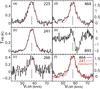 |
Fig. 1 a)–e) HDO spectra observed with APEX. The red lines indicate the results of the Gaussian fit. f) Comparison of the HDO 464 and 241 GHz spectra. The numbers in the plots indicate the observed frequencies (in GHz). The gray vertical lines are at VLSR = 58 km s-1. |
Properties of the HDO lines.
3. First results
3.1. Single-dish observations
The spectra observed toward G34.26+0.15 are presented in Fig. 1. All transitions are detected. They all appear in emission, except for the 893 GHz line, which shows a complex profile, dominated by an absorption component. This is because the 893 GHz line is a ground transition and has a high critical density. The line profiles of the three high-excitation transitions (225, 241, and 266 GHz) are close to Gaussian and their linewidths are ~6.3−6.7 km s-1, obtained from a Gaussian fit. Not only are the profiles of 225 and 241 GHz HDO lines very similar, but their intensities are very close to each other. The linewidth of the 464 GHz HDO line is slightly wider than the high-excitation lines (~7.2 km s-1), although this does not appear to be significant, owing to the large error bars, and as shown in Fig. 1f, which displays the superposition of the 464 and 241 GHz line profiles. It is found that the difference between these two spectra is still within the 3σ noise level, and that there is no obvious evidence for the existence of a broad component in the 464 GHz line, as was found in some ground transition H2O lines (Kristensen et al. 2010b; Chavarría et al. 2010).
Table 2 lists the properties of the observed HDO
lines. Using the integrated line intensities, we performed a rotation diagram analysis
assuming that the lines are optically thin and in local thermodynamic equilibrium (LTE)
(Goldsmith & Langer 1999). We considered only
the three high-excitation lines, because the two ground-state lines are suggested to be
optically thick (see Sect. 4.3). We assumed a 1″ source size, as suggested from the
interferometric observations (Table 3). Because
this size is smaller than the three observational beams, the derived column density and
source size are degenerate, and the temperature does not depend on the size assumption.
The resulting rotation diagram is displayed in Fig. 2. The rotation temperature obtained is
~ K, which is consistent with the estimates
of the kinetic temperature (160 ± 30 K) from the analysis of OCS, CH3OH, SO,
and HC3N (Mookerjea et al. 2007). The
derived total molecular column density of the hot HDO is
4.1 × 1017 cm-2 averaged on the assumed 1′′ extended source.
K, which is consistent with the estimates
of the kinetic temperature (160 ± 30 K) from the analysis of OCS, CH3OH, SO,
and HC3N (Mookerjea et al. 2007). The
derived total molecular column density of the hot HDO is
4.1 × 1017 cm-2 averaged on the assumed 1′′ extended source.
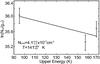 |
Fig. 2 HDO rotation diagram. The detected lines are shown as crosses with error bars. The size of the error bars corresponds to 20% of the intensity due to the calibration uncertainty. |
Results of the SMA observations
3.2. Interferometer observations
3.2.1. Continuum at λ = 1.3 mm
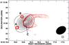 |
Fig. 3 Overlay of the 1.3 mm continuum emission observed with the SMA (black contours)
with the red contours of the 43.3 GHz free-free continuum emission observed by
Avalos et al. (2006). Contour levels are
from 3σ by steps of 6σ, with 1σ
= 0.1 Jy beam-1 for the SMA images and at −4, −3, 3, 4, 5, 6, 8, 10,
12, 15, 20, 40, 60, 100, 200, 400, and 800 times the noise, with
1σ = 1.04 mJy beam-1 for the 43.3 GHz images. The
synthesized beams of the SMA (black) and free-free emission (red) images are shown
in the lower right of the plot. The synthesized beam of the 2-cm image is
1 |
The total continuum flux retrieved within the SMA primary beam is 8.0 Jy. The continuum emission is found to be slightly resolved (Table 3). Figure 3 shows an overlay of the 1.3 mm continuum image with the free-free continuum emission observed by Avalos et al. (2006). The continuum peak detected at 1.3 mm does not coincide with HII regions A and B, but is roughly consistent with HII region C within the beam size (detail see Fig. 4). At 107 GHz, the integrated continuum intensity of 6.7 Jy is suggested to be dominated by free-free emission and only ~10% can be contributed from dust (Mookerjea et al. 2007). To date, neither the turnover point of free-free emission nor the spectral index are clear. Thus, if the free-free emission is already optically thin at a wavelength longer than 3 mm, the free-free emission will contribute ~6 Jy to the emission at 1.3 mm. In other words, the detected continuum flux with the SMA is the combination of free-free and dust emission. Figure 4 also supports this argument, because the peak of the 1.3 mm continuum is located between the peak of the free-free emission (from which it is offset by ~0.3″) and the HDO peak. This point will be important when modeling the emission with RATRAN (which models only the dust continuum).
3.2.2. Spectral lines
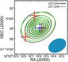 |
Fig. 4 HDO 225 GHz (black contours) and HDO 241 GHz (green-dashed contours) integrated map observed with the SMA. The contour levels are from 3σ by steps of 6σ, with 1σ = 1.5 Jy beam-1. The red crosses indicate the peak of the 24 GHz free-free continuum emission (A, B, and C positions from Heaton et al. 1989) and the peak (maximum pixel) of the 1.3 mm continuum observed with the SMA is shown with the dark blue cross. The blue ellipse indicates the beam size. |
The observational results for the two HDO lines are listed in Table 3. The integrated intensity maps of the two HDO lines (Fig. 4) show that their emission distributions are similar, suggesting that the emission comes from the same gas. In addition, the emission is not coincident with the A and B compact HII regions. The peak of the HDO emission is offset from the 1.3 mm dust continuum peak by approximately 0.3−0.4′′ (Table 3), under the theoretically positional error of approximately 0.04′′ with a signal-to-noise ratio (S/N) of 43. We believe that this offset is significant, because the continuum and the lines were observed simultaneously. This offset seems to be much smaller than the offset (2′′) observed for CH3CN by Watt & Mundy (1999), and on the lower end of the different offsets observed for different molecules (CH3OH, SO, and OCS) by Mookerjea et al. (2007). Those molecules have lower critical densities2 compared to the two HDO lines, so excitation effects might partly explain the discrepancy between the distribution of the molecules.
Comparing the results observed with APEX, we find that the missing flux of the HDO 225 GHz and 241 GHz line emission are ~37.1% and ~36.4%, suggesting that most HDO emission is coming from the center of the molecular cloud core, which is consistent with the fact that the line shapes are very similar. Here, the SMA map was convolved with the beam size of APEX. The calibration uncertainties of APEX and SMA are usually considered to be ~20% and 5−15%. It is difficult to believe that the apparent missing flux is real, because that would require that these high-excitation HDO lines show some extended emission, which is very unlikely in view of their critical density and energy. Indeed, the differences in fluxes between the SMA and APEX spectra can be also caused by the side lobes in the SMA images. Because the declination (δ2000) of our source is around 1 degree, the side lobes are quite strong and cannot be easily removed thoroughly. The negative side lobes will lower the obtained integrated flux (SMA) in this case. We therefore assume that the flux discrepancy is only originating in the uncertainty of the calibration and imaging of the data.
We resolved the CN 2–1 hyperfine structure of J = 3/2−1/2 and J = 5/2−3/2. All CN absorption lines show redshifted absorption; we discuss in more detail in Sect. 5.2.2.
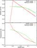 |
Fig. 5 Comparison of the physical profiles of the two different models toward G34.26+0.15 (Nomura & Millar 2004; Rolffs et al. 2011). |
4. Modeling
4.1. Physical profiles of the source
To analyze the HDO data, we used the 1 D Monte Carlo code RATRAN, developed by Hogerheijde & van der Tak (2000). The radiative transfer model takes as input the physical (n, T) profiles of the source. The heating source of the hot core and its density structure are not clearly understood toward G34.26+0.15, because there is no high angular resolution study (≤ 1″) in the submillimeter band. It has been argued that the hot core could be externally heated by this HII region (Mookerjea et al. 2007), because the hot core lies off the cometary-shaped HII region (Watt & Mundy 1999). This cometary-shape may be caused by the bow shock produced by the wind from a young star that moves at supersonic speed through an ambient molecular cloud (Wood & Churchwell 1989; van Buren et al. 1990; Watt & Mundy 1999) or by the champagne outflow (Andersson & Garay 1986; Fey et al. 1992; Carral & Welch 1992; Gaume et al. 1994). The separations between the HII region and the emission peaks of most N- and O-bearing molecules are ≤1″ (Mookerjea et al. 2007, see Fig. 3). However, recent studies with HCN, HCO+, CO, and their isotopes observed with APEX show no evidence for this scenario and, moreover, the results show self-absorption and strong red asymmetries, which suggest an in-falling source with internal heating (Rolffs et al. 2011). In addition, the studies of the NH3 (32−22) line observed with SOFIA also present a clear in-fall absorption in the spectra which are well reproduced also with Rolffs’ model (Wyrowski et al. 2012). This may be because they probe larger scales and the structures of the heating area are too small to be resolved in their observations (Rolffs et al. 2011). Therefore, the external heating structures could be internal in the model. Neither our APEX nor our SMA data have a sufficiently high resolution to probe the scale of the heating region; therefore, the two models we adopted here have the temperature structures derived by the inner heating source.
We use in the following the physical profiles of two different models (Nomura & Millar 2004; Rolffs et al. 2011, Fig. 5).
Nomura’s model is constrained by the observed spectral energy distribution (SED) data at
wavelengths from far-infrared to millimeter. Most data are from Chini et al. (1987) and were observed with the ESO 1 m telescope, except
for an additional point at around 3 mm (Nomura &
Millar 2004, see Fig. 1c). The 3-mm data point is taken from Watt & Mundy (1999) and were observed with BIMA
(Nomura, private communication). As in Nomura’s study, the model with the column density
of N = 1025 cm-2 is used here. The density and
temperature profiles of the Rolffs model aim to reproduce the radial intensity profile
from LABOCA data (345 GHz continuum). We adopted the opacity and velocity field setting of
the Rolffs model for both models (opacity: ice mantle coagulation at a density of
105 cm-3, Ossenkopf & Henning
1994; velocity field: 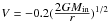 , Rolffs
et al. 2011). The turbulent linewidth, db, is set to be 3.0 km s-1.
The adopted distance is 3.7 kpc (Kuchar & Bania
1994). The HDO collisional rates used in this study are computed by Faure et al. (2012) for para-H2 and
ortho-H2 separately. In the modeling, we assumed that the ortho-to-para ratio
of H2 is in LTE in each cell of the core.
, Rolffs
et al. 2011). The turbulent linewidth, db, is set to be 3.0 km s-1.
The adopted distance is 3.7 kpc (Kuchar & Bania
1994). The HDO collisional rates used in this study are computed by Faure et al. (2012) for para-H2 and
ortho-H2 separately. In the modeling, we assumed that the ortho-to-para ratio
of H2 is in LTE in each cell of the core.
Fitting parameters and their results.
4.2. Modeling procedure
The HDO emission was modeled with a jump model, where the fractional abundances of
deuterated water, relative to H2, in the inner part of the source
(T > 100 K, assumed evaporation temperature) and in the outer
part (T ≤ 100 K) are two free parameters,
X and
X
and
X . We made two sets of comparisons, one with
the APEX data and the other with the SMA data. For comparison with the APEX data, the
modeled maps were convolved with the APEX beam. For comparison with the SMA data, we used
MIRIAD to create mock observations based on the modeled data. We first inserted the values
of the observed parameters (epoch, rest frequency, and the coordinate of the observed
reference position) into the blank header of the modeled data. Then, we multiplied the
modeled image by the SMA primary beam. Afterward, we applied the (u,
v) sampling retrieved from the SMA data to the modeled image and
inverted the resulting (u, v) data to obtained the
simulated maps/spectra. We then performed χ2 analyses for
X
. We made two sets of comparisons, one with
the APEX data and the other with the SMA data. For comparison with the APEX data, the
modeled maps were convolved with the APEX beam. For comparison with the SMA data, we used
MIRIAD to create mock observations based on the modeled data. We first inserted the values
of the observed parameters (epoch, rest frequency, and the coordinate of the observed
reference position) into the blank header of the modeled data. Then, we multiplied the
modeled image by the SMA primary beam. Afterward, we applied the (u,
v) sampling retrieved from the SMA data to the modeled image and
inverted the resulting (u, v) data to obtained the
simulated maps/spectra. We then performed χ2 analyses for
X ranging from 1 × 10⁻⁹ to
4 × 10⁻⁷ and for X ranging from 1 × 10-15 to
2 × 10-11 for the Rolffs model and for
X ranging from 1 × 10-12 to
5 × 10⁻⁹ and for X ranging from 1 × 10-17 to
5 × 10⁻¹⁰ for the Nomura model. We intend to also model the line velocity
profiles and all spectra, including the spectra from the SMA data. Here the definition
of χ2 is
ranging from 1 × 10⁻⁹ to
4 × 10⁻⁷ and for X ranging from 1 × 10-15 to
2 × 10-11 for the Rolffs model and for
X ranging from 1 × 10-12 to
5 × 10⁻⁹ and for X ranging from 1 × 10-17 to
5 × 10⁻¹⁰ for the Nomura model. We intend to also model the line velocity
profiles and all spectra, including the spectra from the SMA data. Here the definition
of χ2 is  , where the sum is over each channel in
each spectrum. The σ within this χ2 analysis
includes the statistical errors and uncertainties in flux calibration (~10% for 225
and 241 GHz observed with SMA, ~30% for 893 GHz and ~20% for other lines
observed with APEX), but does not include any uncertainty in the adopted collisional rate
coefficients used in the excitation calculation (Faure
et al. 2012).
, where the sum is over each channel in
each spectrum. The σ within this χ2 analysis
includes the statistical errors and uncertainties in flux calibration (~10% for 225
and 241 GHz observed with SMA, ~30% for 893 GHz and ~20% for other lines
observed with APEX), but does not include any uncertainty in the adopted collisional rate
coefficients used in the excitation calculation (Faure
et al. 2012).
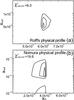 |
Fig. 6 X |
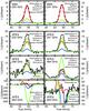 |
Fig. 7 Comparison of the observed spectra with the results of our best-fit models for the
two different physical profiles. The observed line emission is shown as black
histograms in each spectrum. The red, green, and blue lines show the best-fit
results of the Rolffs model, the Nomura model with all spectra, and the Nomura model
excluding the HDO spectrum at 893 GHz (X |

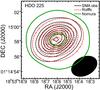 |
Fig. 8 Overlay of the HDO 225 GHz integrated map observed with the SMA (black contours) with the simulated ones of the best-fit results of the Rolffs model and of the Nomura model excluding the HDO spectrum at 893 GHz. The red and green contours show the integrated HDO 225 GHz map of the best-fit results of the Rolffs model and of the Nomura model excluding the HDO spectrum at 893 GHz. These two integrated maps are simulated to be observed with the uv-coverage of the SMA observations. All contour levels are from 3σ by steps of 5σ, with 1σ = 1.5 Jy beam-1. The black ellipse indicates the beam size. |
4.3. Results
The black solid lines in Fig. 6 present the contours
delimitating the 1σ (68.3%), 2σ (95.4%) and
3σ (99.7%) confidence intervals. These contours are derived with the
method described in Lampton et al. (1976), who
showed that the  random variable follows a
χ2 distribution with p variables,
p being the number of parameters. Here p = 2
(Xin and Xout), so that these contours correspond to
χ2 =
random variable follows a
χ2 distribution with p variables,
p being the number of parameters. Here p = 2
(Xin and Xout), so that these contours correspond to
χ2 =  +2.3,
+6.17 and
+11.8. Here we used 1σ,
2σ, and 3σ in analogy with Gaussian-distributed random
variables.
+2.3,
+6.17 and
+11.8. Here we used 1σ,
2σ, and 3σ in analogy with Gaussian-distributed random
variables.
The fitting parameters and obtained results are listed in Table 4. The observed spectra are overlaid with the modeling results of the
best fit in Fig. 7. Here the system velocity of
58 km s-1 is assumed (VLSR). The minimum
 are not close to 1, which indicates that
the spectra are not well reproduced by the two different physical models. This is also
obvious in Fig. 7. When the Rolffs model is adopted
(red lines in Fig. 7), the emission at 225, 241, and
266 GHz is not high enough at the large scale to fit the observed data (APEX data), but
the most compact emission in the 225 and 241 GHz lines is well reproduced (SMA data). At
the same time, the simulated spectra at 464 and 893 GHz are optically thick
(τ = 2.1 and τ = 24.1 at lines and source center) and
the line profile in 893 GHz spectrum does not fit the observed spectrum either. In
Fig. 7, the blue and green lines indicate the
results of the best-fit model using the Nomura physical profile, the green line was
obtained excluding the spectrum at 893 GHz from the χ2
analysis. In this case, the fractional abundances are 2 × 10⁻⁹ and
5 × 10-12 for the inner and outer region. This model fails to reproduce the
central emission observed with the SMA.
are not close to 1, which indicates that
the spectra are not well reproduced by the two different physical models. This is also
obvious in Fig. 7. When the Rolffs model is adopted
(red lines in Fig. 7), the emission at 225, 241, and
266 GHz is not high enough at the large scale to fit the observed data (APEX data), but
the most compact emission in the 225 and 241 GHz lines is well reproduced (SMA data). At
the same time, the simulated spectra at 464 and 893 GHz are optically thick
(τ = 2.1 and τ = 24.1 at lines and source center) and
the line profile in 893 GHz spectrum does not fit the observed spectrum either. In
Fig. 7, the blue and green lines indicate the
results of the best-fit model using the Nomura physical profile, the green line was
obtained excluding the spectrum at 893 GHz from the χ2
analysis. In this case, the fractional abundances are 2 × 10⁻⁹ and
5 × 10-12 for the inner and outer region. This model fails to reproduce the
central emission observed with the SMA.
Comparing the results reproduced by the two models (red and blue), we find that the best
fit based on the Rolffs model is closer to the observed data
( ). The fitting problems in the ground
transitions (464 and 893 GHz) are slightly less severe than for the Nomura model (see
Fig.7). Moreover, from the comparison of the two
fitting results of the Nomura model (blue and green), we find that the absorption in the
893 GHz spectra and emission in 464 GHz are too strong if we try to increase the emission
in the high-excitation lines to fit the spectra (225, 241, 266 GHz). Indeed, the continuum
flux reproduced with the Nomura model (~49 K) is much higher than the real flux
(~13.0 K). This is also found in Appendices A.2. and A.3. Figure 8 shows the angular distribution of the 225 GHz line from the SMA
observation and the two models. Here again the model based on the Rolffs profiles fits the
data much better. This is similar for the 241 GHz line and is therefore not shown.
). The fitting problems in the ground
transitions (464 and 893 GHz) are slightly less severe than for the Nomura model (see
Fig.7). Moreover, from the comparison of the two
fitting results of the Nomura model (blue and green), we find that the absorption in the
893 GHz spectra and emission in 464 GHz are too strong if we try to increase the emission
in the high-excitation lines to fit the spectra (225, 241, 266 GHz). Indeed, the continuum
flux reproduced with the Nomura model (~49 K) is much higher than the real flux
(~13.0 K). This is also found in Appendices A.2. and A.3. Figure 8 shows the angular distribution of the 225 GHz line from the SMA
observation and the two models. Here again the model based on the Rolffs profiles fits the
data much better. This is similar for the 241 GHz line and is therefore not shown.
The model based on the Rolffs centrally heated core reproduces the SMA observed line distribution well. This does not exclude the possibility that the heating of the very central dust core is external, but it shows that even at the resolution of our SMA data, we do not see clear evidence of a non-spherically symmetric heating of the envelope, and that the large-scale properties of the envelope can therefore be derived using such a model. Distinguishing between internal and external heating at small scales would require observations with much higher angular resolution.
Based on the superior results obtained with the Rolffs profiles, we focus on the Rolffs model below and try to reproduce the lines with a two-jump model of the HDO abundance distribution. Finally, we modify Rolffs physical structure to try to fit the observed data. The results of the two-jump model and modified models are discussed in Sects. 5.1 and 5.2 and in Appendices A.2. and A.3.
5. Discussion
5.1. Two-jump model
To reproduce more emission in the high-excitation lines and decrease the emission in the 893 GHz line, we modeled the spectra with a two-jump model instead of a one-jump model. The additional jump was arbitrarily set to be located at T = 200 K. Figure 9 show the results of four testing models. The adopted HDO fractional abundances of the models are listed in Table 5. The red lines indicate the results of the original best-fit one-jump model, which underestimates the high-excitation lines. The two-jump models (2J-1 and 2J-3) are found to be somewhat better for these transitions (Fig. 9). This suggests that the two-jump model can produce higher emission in the high-excitation lines. This property has already been found for Sgr B2 (M) (Comito et al. 2010) and this is due to the very high critical density of these lines (see Table 1). Moreover, although we decreased the HDO fractional abundance in the second inner region of the core in model 2J-2 and 2J-4 by a factor of 2, the emission in the 893 GHz line is little affected (<1σ). In addition, the line shapes of different lines do not change from model to model. Therefore, the results suggest that adopting a two-jump model can help in increasing the emission in the high-excitation lines, but cannot improve the 893 and 464 GHz line shapes. We note, however, that because the inner part is very compact, the enhancement of the high-excitation lines in the APEX beam when increasing the HDO abundance in this inner part is linked to an even faster relative enhancement of the flux in the SMA beam. As a consequence, one cannot increase the inner HDO abundance too much, even if the effect on the APEX lines is almost unnoticeable.
Parameters of the models.
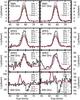 |
Fig. 9 Comparison of the observed spectra and those simulated with different models. The red lines are the spectra of the original one-jump model. |
5.2. Modified physical profiles
In the previous sections, we have seen that the observed spectra are not perfectly reproduced using the Rolffs physical profile, even with a two-jump model. This is also the case for some HCN lines (see Fig. 5 in Rolffs et al. 2011). We now investigate how the model can be improved by modifying the physical profiles from the Rolffs model. We first investigate where the HDO emission and absorption take place by means of a shell analysis and then test the effect of modfying the physical profiles of the Rolffs model.
5.2.1. Shell analysis and modified density/temperature profiles
To analyze the discrepancy between the best-fit model and the observed data, we performed a shell analysis by sequentially turning the abundance of HDO in the innermost shells to 0 and then simulating new spectra (Fig. A.1). The results of this study are shown in Appendix A.1. We find that the emission of all transitions (even the 893 GHz line) originates in the inner region, whereas the absorption originates in the outer region. This explains why it is impossible to improve the line profile of the 893 GHz within the frame of a jump model. Improvement can therefore only be achieved by modifying the physical profiles (density, temperature, velocity) of the source. In Appendices A.2 and A.3, we show that modifications of the density and temperature profiles are unable to improve the quality of the fit. In the next section, we investigate the effect of modifying the velocity field.
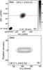 |
Fig. 10 Integrated moment-0 map of CN 2-1 J = 5/2−3/2 F = 7/2−5/2 line (blended with the F = 5/2−3/2 and F = 3/2−1/2 lines) overlaid with the dust continuum map a). The red line indicates the cut for the position-velocity (P − V) diagram. The P − V diagram of the CN line b). Both are observed with SMA. The contours in a) are −0.67, −1.34, −2.01, −2.68, −3.35, and −4.02 and in b) they are −0.97, −1.94, −2.91, −3.88, −4.86, and −5.83. The P − V diagram is cut at the position of the observed center and position angle of 0. |
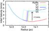 |
Fig. 11 Comparison of the velocity profiles of the four different modified models (green, blue, purple, and light-blue) and the one of the Rolffs original model (red). |
5.2.2. Modified velocity profile
– Modified infall velocity field So far, we used the velocity profile provided by Rolffs et al. (2011) for all modeling. This is a modified free-fall velocity field. However, the line shape in the 893 GHz spectra cannot be simply reproduced by our present model, which might imply that there is an additional velocity field in the core.
Figure 10 shows the moment-0 map overlaid with
the dust continuum map (a) and the position-velocity diagram (b) of the CN 2–1
absorption line observed with the SMA simultaneously to the HDO lines. Clearly, the
distribution of the CN absorption is consistent with that of the dust continuum, as in
the case of HDO. Moreover, the central velocity of the position-velocity diagram of the
CN absorption is about 61 km s-1, not 58 km s-1. This redshifted
absorption has already been found for many molecules, for instance NH3, CO,
13CO, and HCO+ (Heaton et al.
1989; Gómez et al. 2000; Wyrowski et al. 2012). Thus, it is possible that the
gas that produces the absorption feature in the HDO 893 GHz spectra has a similar
velocity distribution. Therefore we tried to modify the velocity field by adding a
3 km s-1 difference from the outer region to the inner region of the core
(Fig. 11). The results are shown in Fig. 12. The spectra are simulated with the fixed
fractional abundances 6 × 10⁻⁸ (X) and 5 × 10-12
(X ) (best-fit model). The additional
velocity (3 km s-1) widens the emission of the optically thin lines (225,
241, and 266 GHz) somewhat, which enables a better fit of the line-width of the SMA
lines. The opacities of the HDO 464 and 893 GHz lines are reduced and the 464 GHz line
becomes optically thinner in models V3 and V4 (τ = 1.3 and 0.8).
Moreover, the peak positions of the absorption in the simulated 893 GHz spectra
gradually approach those of the observed 893 GHz spectra. Therefore, carefully modifying
the velocity field might be a good way to improve the fits. However, the detailed
velocity profile around the boundary region of the core cannot be constrained from our
data now. To obtain better modeling results, it is necessary to observing the HDO line
map at 893 GHz with high angular resolution. In addition, this result also suggests that
studying the HDO spectrum at 893 GHz can help us to understand the velocity field of the
core.
) (best-fit model). The additional
velocity (3 km s-1) widens the emission of the optically thin lines (225,
241, and 266 GHz) somewhat, which enables a better fit of the line-width of the SMA
lines. The opacities of the HDO 464 and 893 GHz lines are reduced and the 464 GHz line
becomes optically thinner in models V3 and V4 (τ = 1.3 and 0.8).
Moreover, the peak positions of the absorption in the simulated 893 GHz spectra
gradually approach those of the observed 893 GHz spectra. Therefore, carefully modifying
the velocity field might be a good way to improve the fits. However, the detailed
velocity profile around the boundary region of the core cannot be constrained from our
data now. To obtain better modeling results, it is necessary to observing the HDO line
map at 893 GHz with high angular resolution. In addition, this result also suggests that
studying the HDO spectrum at 893 GHz can help us to understand the velocity field of the
core.
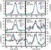 |
Fig. 12 Comparison of the observed and modeled spectra using the velocity profiles V1-V4 (Fig. 11) and the same HDO fractional abundance as in the best fit. The red lines are the spectra modeled with the best-fit model using the original Rolffs physical profile. The observed and fitting spectra at 241 GHz are very similar to the those at 225 GHz; therefore, only the spectra at 225 GHz are plotted here. |
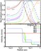 |
Fig. 13 HDO normalized population of the selected levels of the Rolffs original model a) and comparison of the turbulent velocity fields of the four models (db1 – db4) and the turbulent velocity fields of the original model (red) b). |
– Modified turbulence velocity width Because the line profiles are also affected by gas
motions, the turbulence is also responsible for the line emission/absorption widths. The
assumption that turbulence varies over the core has already been used for analyzing the
spectra lines toward several massive sources and brought nicely fitting results (Herpin et al. 2009). Our previous study shows that
the width of all simulated 893 spectra is obviously much wider than that of the observed
spectrum, while the widths of the high-excitation lines are well fitted. Thus, we
modified the turbulent velocity field by changing the parameter db in the model. In the
Fig. 13a, the distribution of the populations of
the upper level of high-excitation lines (31,2, 22,0, and
22,1) is different from those of the ground-transition lines
(11,1 and 10,1). The peaks of the high-excitation line
populations are mainly located in the layer 15−16
(1.4 × 10⁻² − 1.7 × 10⁻² pc) and those of the
ground-transition lines are placed in the layer 21−24
(6.4 × 10⁻² − 1.0 × 10⁻¹ pc). We used these
considerations for elaborating our new db settings with the aim to narrow down the width
of the simulated 893 spectra without significantly affecting the width of the
high-excitation lines. Figure 13b illustrates our
different db settings. The HDO fractional abundances in the model db1 – db4 are fixed
with the values of the best-fit model: X and
X
and
X .
.
Comparing the spectra at 893 GHz with those of the previous best-fit model (Fig. 14), we find that the line profile has significantly
improved much in db2 – db4. The width of the absorption part is narrower than before and
more similar to the observed one. Moreover, we have better fits compared to previous
spectra at 266 GHz and the opacity is reduced in the 464 GHz spectra. In addition, the
model db2 is 5.5, which is better than
that of the Rolffs original model (6.0), showing that the fits can be improved by
modifying the turbulent velocity field. We also performed χ2
analyses for the same range of X and
X in Sect. 4.2 based on model db2. The
fractional abundances of the new best-fit in this test are still the same as in our
previous results (X and
X
and
X ). This implies that the turbulence
velocity is not constant throughout the envelope of G34.26+0.15. However, the widths at
225 and 241 GHz are narrower than the previous and observed ones, suggesting that the db
in the inner region of the core is not wide enough in the models. Here again, high
angular resolution data at 893 GHz would be very helpful.
). This implies that the turbulence
velocity is not constant throughout the envelope of G34.26+0.15. However, the widths at
225 and 241 GHz are narrower than the previous and observed ones, suggesting that the db
in the inner region of the core is not wide enough in the models. Here again, high
angular resolution data at 893 GHz would be very helpful.
– Composition of the turbulent and infall velocity field effects Because modifying the infall velocity field can help to move the peak of the absorption at 893 GHz (model V1), and modifying the turbulence velocity field can narrow this absorption, we ran models with modified velocity (V1 and db2). The result is shown in Fig. 15. Obviously, we can now reproduce part of the emission and all the absorption with better width and proper position, which allows us to study the fractional abundance in the outer region of the core. On the other hand, as expected, the emission at 893 GHz is not reproduced properly, because it originates from the inner region of the core (T > 100 K) and the model V1 only changes the velocity field in the outer region of the core (T < 100 K). Additional constraints in this direction will hopefully come from interferometeric data.
In conclusion, we have shown that it is possible to improve the original best-fit model by modifying the velocity field of the source. This improvement is obtained while keeping the fractional abundance of HDO to the value we derived with the original velocity setup of Rolffs et al. (2011). This study confirms the validity of the fractional abundance of HDO derived from the best-fit model in Sect. 4.3. Further steps toward constraining the velocity field and therefore a better HDO model will need high angular resolution observations of, e.g., the HDO 893 GHz line.
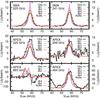 |
Fig. 14 Same as Fig. 12, but for the models with different settings of the turbulent velocity field (db1 – db4). |
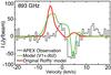 |
Fig. 15 Comparison of the observed spectrum, the one of the best-fit model simulated with Rolffs’ original physical profile, and the one reproduced with the modified turbulent and infall velocity fields (V1 and db2). The fractional abundance adopted here is the one of the best-fit model. |
5.3. HDO/H2O ratio
O is always used to trace H2O,
because H2O is easily optically thick. Here we compare the emission and
absorption of the two para-O lines 313 − 220 and
111 − 000 (Gensheimer et al.
1996; Wyrowski et al. 2010) with our HDO
results. Because the analysis of the HDO lines suggests that high-excitation lines can
trace and constrain the inner fractional abundance quite well (Parise et al. 2005b; Liu et al.
2011), we can also analyze the high-excitation
O 313 − 220 line
(Eu = 204.7 K) (Gensheimer
et al. 1996) to study the O fractional abundance in the inner region
of the core. We reproduced the reported integrated flux and line width (20.5 K and
8.4 km s-1 listed in Table 2 in Gensheimer
et al. 1996) of this O line with RATRAN using a one-jump model
based on the Rolffs original profiles. The resulting fractional abundance of the
para-O in the inner region of the core is
(1.0 ± 0.7) × 10-7 (3σ). Thus, the HDO/H2O is
3.0 × 10⁻⁴ with the assumption that the standard ortho/para ratio is 3 and
the 18O/16O ratio is 500. This ratio is consistent with the estimate
of 1.1 × 10⁻⁴ with an uncertainty of a factor of 4 (Gensheimer et al. 1996). Here, the adopted db for this high-excitation
O line is 4.5 km s-1 instead of
3 km s-1, because the width of this O line is wider than that of the
high-excitation HDO lines (8.4 km s-1 for the
O line compared to
~6−7 km s-1 for the HDO lines). The different properties of the
velocity field of the high-excitation O line may indicate that some part of the
emission does not come from the quiescent envelope and the high-excitation HDO lines may
not probe exactly the same gas. Therefore, the derived D/H ratio of water in the inner
region here should be a lower limit.
Figure 16 displays the two spectra of the
ground-state 11,1 − 00,0 transition of HDO and
O. The line shapes are very similar,
suggesting they may originate from the same gas. Under the two assumptions that the
excitation temperature of the line is negligible with respect to the temperature of the
background continuum source and that only the ground state of the molecule is populated,
the total column density of the absorbing HDO/O can then be computed from (Comito et al. 2003; Tarchi et al. 2004)  (1)where Δv is the line width
and gl and
gu are the statistical weights of the
lower and upper level. The optical depth of the absorbed line can be determined by
(1)where Δv is the line width
and gl and
gu are the statistical weights of the
lower and upper level. The optical depth of the absorbed line can be determined by
 (2)where TL is the
brightness temperature of the line and TC is the brightness
temperature of the continuum. The line parameters from the Gaussian fit and the estimated
values are listed in Table 6. The estimated total
column densities are 1.8 × 1012 cm-2 for HDO and
1.8 × 1012 cm-2 for para-O. Because the profiles of these two lines
are very similar to each other, we assumed that both of them are originating from the same
gas. Therefore, the [HDO]/[H2O] ratio is ~4.9 × 10⁻⁴, assuming
that the standard ortho/para ratio is 3 and the 18O/16O ratio is
500. However, the abundance of para-O might be underestimated here, because the
emitted area of the continuum at 1101 GHz might be larger than that of the
O due to the large Herschel
beam. Assuming that the dust emissivity spectral index β is 2 as
for the interstellar medium (Draine & Lee 1984;
Schnee et al. 2010), the derived continuum flux
at 1101 GHz of the core seen with APEX will be 2.8 K in the Herschel beam
and the estimated total column O density becomes
4.7 × 1012 cm-2. Then the obtained D/H ratio of water is
~1.9 × 10⁻⁴, which is close to what we obtained for the inner region of
the core. We note that this value is uncertain, as the absorption takes place on top of
emission in both cases, which we have ignored here.
(2)where TL is the
brightness temperature of the line and TC is the brightness
temperature of the continuum. The line parameters from the Gaussian fit and the estimated
values are listed in Table 6. The estimated total
column densities are 1.8 × 1012 cm-2 for HDO and
1.8 × 1012 cm-2 for para-O. Because the profiles of these two lines
are very similar to each other, we assumed that both of them are originating from the same
gas. Therefore, the [HDO]/[H2O] ratio is ~4.9 × 10⁻⁴, assuming
that the standard ortho/para ratio is 3 and the 18O/16O ratio is
500. However, the abundance of para-O might be underestimated here, because the
emitted area of the continuum at 1101 GHz might be larger than that of the
O due to the large Herschel
beam. Assuming that the dust emissivity spectral index β is 2 as
for the interstellar medium (Draine & Lee 1984;
Schnee et al. 2010), the derived continuum flux
at 1101 GHz of the core seen with APEX will be 2.8 K in the Herschel beam
and the estimated total column O density becomes
4.7 × 1012 cm-2. Then the obtained D/H ratio of water is
~1.9 × 10⁻⁴, which is close to what we obtained for the inner region of
the core. We note that this value is uncertain, as the absorption takes place on top of
emission in both cases, which we have ignored here.
Line parameters and continuum temperature corresponding to the frequency of each line.
Comparison of HDO fractional abundance between different sources.
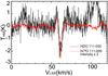 |
Fig. 16 Comparison of the HDO at 893 GHz (black) with
H |

The comparison of the HDO fractional abundances between different sources is shown in Table 7. The water deuterium fractionation toward the two low-mass protostars, NGC1333 IRAS 2A and IRAS 16293-2422, have been studied with several HDO transitions (Liu et al. 2011; Parise et al. 2005a; Coutens et al. 2012). Most transitions were also used in this work.
The abundance of HDO jumps by more than four orders of magnitude at the 3σ confidence level in G34.26+0.15. Similarly to this work, jump models are widely used to analyze the HDO and H2O spectra of other high- and low-mass sources in Table 7, except for Orion KL. Ices are therefore also shown to evaporate from the grains in the inner part of the envelope in protostars of different masses. However, the D/H ratios of water in G34.26+0.15 is much lower than in low-mass protostars and similar to that in AFGL 2591 and other high-mass sources, such as Ori-IRc2, G31.41+0.31, and G10.47+0.03A (van der Tak et al. 2006; Gensheimer et al. 1996). In addition, the D/H ratios of formaldehyde and HCN in G34.26+0.15 are also lower than those in low-mass protostars. This can be explained if the dense and cold pre-collapse phase only lasts a short time and less CO freezes onto grain mantles. This hypothesis has been confirmed in the high-mass source AFGL 2591 (van der Tak et al. 2006).
Figure 17 shows the diagram of HDO/H2O vs. HDCO/H2CO and the values are taken from Table 7. It is found that the fractionation of water is at least ~2.4 times lower than that of formaldehyde. This under-fractionation of water is found to be the most extreme for G34.26+0.15. One possible explanation is that if two molecules are mainly formed on the grain surface, the different deuterium fractionation can be due to the different pathways of each ice formation in translucent clouds: using a very simple chemical network on the grains, Cazaux et al. (2011) showed that the deuteration of formaldehyde is sensitive to the gas D/H ratio during the cloud collapse, while the deuteration of water depends on the dust temperature when ices form. More realistic models including water formation routes involving O2 and O3 also predict a higher fractionation of formaldehyde than water (Du et al. in prep.). However, recent studies showed that formaldehyde can also be formed in the gas phase from photodissociation reactions of grain species (Roueff et al. 2006). Formaldehyde can also efficiently be fractionated in the gas phase up to warm temperatures (~70 K), through the CH2D+ route (Turner 2001; Roueff et al. 2007; Parise et al. 2009). It is therefore likely that the HDCO/H2CO ratio observed in the gas is not directly the result of grain chemistry. A better comparison would be with methanol fractionation, which is generally thought to form essentially on the grains.
Confirming the observed trend of under-fractionation of water would require observationally characterizing the deuterium fractionation (for both water and methanol) toward a bigger sample of sources, spanning a large mass interval. This under-deuteration of water with respect to other species is an important feature, which should be reproduced by astrochemical models aiming at explaining deuterium fractionation.
6. Conclusion
We presented five HDO transitions observed with APEX and two HDO high-excitation
transitions observed with SMA toward the high-mass protostar, G34.26+0.15. With the 1D
radiative transfer code RATRAN, and the physical profiles obtained from Rolffs et al. (2011), we derived the HDO fractional
abundances relative to H2 in the inner and outer region of the core to be
X (T > 100 K) and
X (T ≤ 100 K). This
result shows that the HDO abundance is enriched in the inner region because of the
sublimation of the ice in the same way as for other studied low- and high-mass sources, such
as NGC1333 IRAS 2A, IRAS 16293-2422, and AFGL 2591 (Liu
et al. 2011; Parise et al. 2005a; Coutens et al. 2012; van
der Tak et al. 2006).
(T ≤ 100 K). This
result shows that the HDO abundance is enriched in the inner region because of the
sublimation of the ice in the same way as for other studied low- and high-mass sources, such
as NGC1333 IRAS 2A, IRAS 16293-2422, and AFGL 2591 (Liu
et al. 2011; Parise et al. 2005a; Coutens et al. 2012; van
der Tak et al. 2006).
Although the abundance can be constrained, the HDO line profiles are not well reproduced, especially for the ground-state lines. We found that the fitted emission can be improved with two-jump models, suggesting the enhancement of the fractional abundance in the hot core. Modifying the physical profile, we showed that the velocity field is responsible for the HDO line profile at 893 GHz. Higher angular resolution observations of the HDO 893 GHz line are needed to constrain the velocity profiles of deuterated water in G34.26+0.15.
The H2O abundance is estimated from one high-excitation and one ground transition para-H18O line (Gensheimer et al. 1996; Wyrowski et al. 2010). The D/H ratios of water are 3.0 × 10⁻⁴ in the inner region and (1.9−4.9) × 10-4 in the outer region of the core. The deduced HDO/H2O ratios in G34.26+0.15 are similar to those in other high-mass sources, such as AFGL 2591 (van der Tak et al. 2006), and are much lower than in low-mass star-forming regions, suggesting the possibility that the dense and cold pre-collapse phase is short for high-mass stars. Water is also found to be less fractionated than other molecules such as formaldehyde and methanol. This confirms this characteristic, which was observed previously in other sources, and provides a challenge for chemical models of deuterium fractionation on grain surfaces.
Online material
Appendix A: Model analysis
A.1. Shell analysis
To analyze the discrepancy between the best-fit model based on the Rolffs physical profiles and the observed data for the two ground transitions (464 and 893 GHz), we first constrained the physical shells responsible for the emission and absorption features. To this end, we simulated new spectra by sequentially turning the abundance of HDO in the innermost shells to 0 (Fig. A.1). The jump around 0.02 pc is at the shell whose temperature is about 100 K (jump model) The green dashed line represents the model where the HDO abundance is zero in all inner regions of the core (model SH6). Figure A.2 presents the synthetic spectra obtained with these different models (SH1 – SH6). Obviously there is almost no emission in any spectrum with model SH6, suggesting that all emission, including the emission in the 893 GHz spectrum, is produced in the inner region of the core. Therefore, although loweringn the abundance in the inner region can help to reduce the emission in the 893 GHz line, it will also decrease the emission in other high-excitation lines (225, 241, and 266 GHz). On the other hand, the absorption in the 893 GHz spectrum is entirely produced in the outer region of the core and its line-width is wider than the observed one, implying that the assumed turbulent linewidth is wider than the observed one. Thus, we cannot adequately reproduce all spectra with the Rolffs original physical profiles.
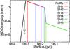 |
Fig. A.1 Original and modified molecular density profiles. The black line shows the original molecular density profile. Different colors indicate different molecular density profiles of models SH1 to SH6. |
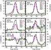 |
Fig. A.2 Comparison of the observed spectra with the results of 6 different shell models (Fig. A.1). Different colors indicate the simulated lines of models SH1 to SH6. The observed and simulated spectra at 241 GHz are very similar to the spectra at 225 GHz; therefore, only the spectra at 225 GHz are plotted here. |
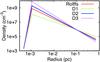 |
Fig. A.3 Comparison of the density profile of the three different modified models (blue, green, and pink) and original Rolffs’ model (red). |
A.2. Modified density profile
From previous test, it was found that the emission in the 893 GHz spectrum cannot be
managed by the Rolffs physical profiles, but only by changing the HDO abundance. We
therefore modified in the first place the density profile of the Rolffs model.
Figure A.3 compares the density profiles of
three different modified models and original the Rolffs model (red line). Here we
modified the density power law index (p), keeping the density at 0.1 pc fixed. The
indices are 1.1 for model D1 (green), 1.7 for model D2 (dark-blue), and 2 for model D3
(purple). Modifying the density profile has a direct impact on the distribution of the
continuum emission. The comparison of the radial profiles of the continuum emission of
different models at multi-wavelength bands (225, 241, 335, and 848 GHz) is shown in
Fig. A.4. Ignoring the misfitting parts within
the beam (orange) and considering that free-free emission most likely also
significantly contributes to the continuum emission, model D1 and the Rolffs model
better reproduce the continuum emission in the 225 and 241 GHz bands than other
models. For the 335 and 848 GHz band, the Rolffs model and all modified models are
superior to the Nomura model. The best-fit results of each model are shown in
Fig. A.5 (model D1:
1.0 × 10⁻⁷(X and
and
 ; model D2:
 and
and
 ; model D3:
 and
and
 ). Comparing all spectra, we find that
model D3 produced intensity similar to the Rolffs model in high-excitation lines and
less emission in the 893 GHz line. However, the 464 and 893 GHz lines are optically
thicker (τ = 2.9 at 464 GHz and τ = 29.6 at 893 GHz)
than the lines produced by the Rolffs model. The high opacities result in
self-absorption in the 464 and 893 GHz spectra (less emission). Moreover, results (464
and 893 GHz spectra) simulated with models D1 and D2 are very similar to the results
produced with the original Rolffs model. Thus, we find that these models are not
significantly better than the original the Rolffs model. In other words, the fits
cannot be improved by simply modifying the density profile.
). Comparing all spectra, we find that
model D3 produced intensity similar to the Rolffs model in high-excitation lines and
less emission in the 893 GHz line. However, the 464 and 893 GHz lines are optically
thicker (τ = 2.9 at 464 GHz and τ = 29.6 at 893 GHz)
than the lines produced by the Rolffs model. The high opacities result in
self-absorption in the 464 and 893 GHz spectra (less emission). Moreover, results (464
and 893 GHz spectra) simulated with models D1 and D2 are very similar to the results
produced with the original Rolffs model. Thus, we find that these models are not
significantly better than the original the Rolffs model. In other words, the fits
cannot be improved by simply modifying the density profile.
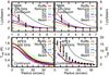 |
Fig. A.4 Radial profiles of the continuum emission at 225 (SMA), 241 (SMA), 356 (LABOCA, Rolffs et al. 2011), and 848 GHz (SABOCA, Wyrowski et al., in prep.) The modified models are overlaid in different colors (model D1 – green, D2 – dark-blue, and D3 – purple). The red and grey lines are reproduced profiles from the original Rolffs’ and Nomura’s models. The beam is shown as a orange dashed Gaussian. The errorbars represent only the deviation from a circular shape. |
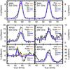 |
Fig. A.5 Comparison of the observed spectra with the best-fit results of 3 different models with modified density profiles (Fig. A.3). The red lines are the best-fit model of the original Rolffs profile. The observed and simulated spectra at 241 GHz are very similar to those at 225 GHz; therefore, only the spectra at 225 GHz are plotted here. |
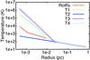 |
Fig. A.6 Comparison of the temperature profiles of the four different modified models (blue, green, light blue and purple) and the one of the original Rolffs model (red). |
A.3. Modified temperature profile
To decrease the emission in 893 GHz spectra and maintain the emission in high-excitation lines (225, 241, 266 GHz), modifying the temperature profile is a possible way. We increased the temperature in the very inner region (models T1, T3, and T4) of the core and decreased the fractional abundance in the inner region of the core. The modified and original temperature profiles are shown in Fig. A.6. Model T2 contrasts with other models.
Like for changing the density profile, modifying the temperature profile also influences the continuum emission. Figure A.7 compares the radial profiles of the continuum emission of different models in the four bands. Again, we find that the Rolffs model and all modified models are superior to the Nomura model in all bands. For the 225 and 241 GHz band, model T2 and the Rolffs model fit better, because the dust continuum is less than 25% of the total continuum flux, implying that increasing the temperature in the central region of the core is a poor solution. In the 335 and 848 GHz bands, T1, T2, and the Rolffs models are superior to others. The indistinguishable continuum at 848 GHz is due to a combination of optical depth and beam dilution effect: the temperature profile is changed only in the very central region of the core where the opacity is high and the beam size is much larger than the scale of the modified region (beam is ~7.4″ at 848 GHz and 2 × 10⁻² pc corresponds to ~1.1″). For 241 and 225 GHz, the angular resolution is sufficiently high and the opacity sufficiently low to detect the very inner region of the core.
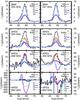 |
Fig. A.8 Comparison of the observed spectra and those reproduced with the fixed fractional abundances of models T1 to T4. The red lines are the best-fit model with the Rolffs original density profile. |
To compare the effect on the spectra, Fig. A.8
shows the fitting results of the different modified models with a fixed HDO fractional
abundance in the inner and outer region (X and
X). The fitting spectra of the T1 and T4
models are similar to spectra of the Rolffs model in the high-excitation spectra at
225 and 241 GHz, while the T2 model produces less emission in all spectra. However,
models T1, T3, and T4 produce much poorer fits to the two ground-transition spectra,
and T2 already becomes optically thick (τ = 3.4) at 464 GHz. Hence,
simply modifying the temperature profiles does not improve the agreement between the
model and the observations.
At 100 K, their critical densities are 1.1 × 10⁵, 3.8 × 10⁶, 6.6 × 10⁴, and 5.3 × 103 cm-3, calculated using the values of the Einstein coefficient and the collision rates tabulated (Green 1986; Pottage et al. 2004; Kristensen et al. 2010a; Green 1994; Green & Chapman 1978; Schöier et al. 2005) in the LAMDA database.
Acknowledgments
The authors warmly thank the anonymous referee and M. Walmsley for very constructive comments and suggestions, which greatly improved this paper. We are grateful to R. Rolffs for many fruitful discussions as well as to F. Herpin for some interesting ideas. We also would like to thank M. Hogerheijde and F. van der Tak for their help in dealing with RATRAN. The authors are grateful to the WISH team for providing access to the H2O data. F.-C. Liu and B. Parise are funded by the German Deutsche Forschungsgemeinschaft, DFG Emmy Noether project number PA1692/1-1.
References
- Andersson, M., & Garay, G. 1986, A&A, 167, L1 [NASA ADS] [Google Scholar]
- Avalos, M., Lizano, S., Rodríguez, L. F., Franco-Hernández, R., & Moran, J. M. 2006, ApJ, 641, 406 [NASA ADS] [CrossRef] [Google Scholar]
- Bergin, E. A., Melnick, G. J., Stauffer, J. R., et al. 2000, ApJ, 539, L129 [NASA ADS] [CrossRef] [Google Scholar]
- Bergin, E. A., Phillips, T. G., Comito, C., et al. 2010, A&A, 521, L20 [NASA ADS] [CrossRef] [EDP Sciences] [Google Scholar]
- Carral, P., & Welch, W. J. 1992, ApJ, 385, 244 [NASA ADS] [CrossRef] [Google Scholar]
- Cazaux, S., Caselli, P., & Spaans, M. 2011, ApJ, 741, L34 [NASA ADS] [CrossRef] [Google Scholar]
- Chavarría, L., Herpin, F., Jacq, T., et al. 2010, A&A, 521, L37 [NASA ADS] [CrossRef] [EDP Sciences] [Google Scholar]
- Chini, R., Kruegel, E., & Wargau, W. 1987, A&A, 181, 378 [NASA ADS] [Google Scholar]
- Comito, C., Schilke, P., Gérin, M., et al. 2003, A&A, 402, 635 [NASA ADS] [CrossRef] [EDP Sciences] [Google Scholar]
- Comito, C., Schilke, P., Rolffs, R., et al. 2010, A&A, 521, L38 [NASA ADS] [CrossRef] [EDP Sciences] [Google Scholar]
- Condon, J. J. 1997, PASP, 109, 166 [NASA ADS] [CrossRef] [Google Scholar]
- Coutens, A., Vastel, C., Caux, E., et al. 2012, A&A, 539, A132 [NASA ADS] [CrossRef] [EDP Sciences] [Google Scholar]
- Cuppen, H. M., Ioppolo, S., Romanzin, C., & Linnartz, H. 2010, Phys. Chem. Chem. Phys. (Incorporating Faraday Transactions), 12, 12077 [NASA ADS] [CrossRef] [Google Scholar]
- Draine, B. T., & Lee, H. M. 1984, ApJ, 285, 89 [Google Scholar]
- Faure, A., Wiesenfeld, L., Scribano, Y., & Ceccarelli, C. 2012, MNRAS, 420, 699 [NASA ADS] [CrossRef] [MathSciNet] [Google Scholar]
- Fey, A. L., Claussen, M. J., Gaume, R. A., Nedoluha, G. E., & Johnston, K. J. 1992, AJ, 103, 234 [NASA ADS] [CrossRef] [Google Scholar]
- Gaume, R. A., Fey, A. L., & Claussen, M. J. 1994, ApJ, 432, 648 [NASA ADS] [CrossRef] [Google Scholar]
- Gensheimer, P. D., Mauersberger, R., & Wilson, T. L. 1996, A&A, 314, 281 [NASA ADS] [Google Scholar]
- Goldsmith, P. F., & Langer, W. D. 1999, ApJ, 517, 209 [NASA ADS] [CrossRef] [Google Scholar]
- Gómez, Y., Rodríguez-Rico, C. A., Rodríguez, L. F., & Garay, G. 2000, Rev. Mex. Astron. Astronfis, 36, 161 [NASA ADS] [Google Scholar]
- Green, S. 1986, ApJ, 309, 331 [NASA ADS] [CrossRef] [Google Scholar]
- Green, S. 1994, ApJ, 434, 188 [NASA ADS] [CrossRef] [Google Scholar]
- Green, S., & Chapman, S. 1978, ApJS, 37, 169 [NASA ADS] [CrossRef] [Google Scholar]
- Hatchell, J., Millar, T. J., & Rodgers, S. D. 1998a, A&A, 332, 695 [NASA ADS] [Google Scholar]
- Hatchell, J., Thompson, M. A., Millar, T. J., & MacDonald, G. H. 1998b, A&AS, 133, 29 [NASA ADS] [CrossRef] [EDP Sciences] [Google Scholar]
- Heaton, B. D., Little, L. T., & Bishop, I. S. 1989, A&A, 213, 148 [NASA ADS] [Google Scholar]
- Herpin, F., Marseille, M., Wakelam, V., Bontemps, S., & Lis, D. C. 2009, A&A, 504, 853 [NASA ADS] [CrossRef] [EDP Sciences] [Google Scholar]
- Hogerheijde, M. R., & van der Tak, F. F. S. 2000, A&A, 362, 697 [NASA ADS] [Google Scholar]
- Jacq, T., Walmsley, C. M., Henkel, C., et al. 1990, A&A, 228, 447 [NASA ADS] [Google Scholar]
- Kristensen, L. E., van Dishoeck, E. F., van Kempen, T. A., et al. 2010a, A&A, 516, A57 [NASA ADS] [CrossRef] [EDP Sciences] [Google Scholar]
- Kristensen, L. E., Visser, R., van Dishoeck, E. F., et al. 2010b, A&A, 521, L30 [NASA ADS] [CrossRef] [EDP Sciences] [Google Scholar]
- Kuchar, T. A., & Bania, T. M. 1994, ApJ, 436, 117 [NASA ADS] [CrossRef] [Google Scholar]
- Lampton, M., Margon, B., & Bowyer, S. 1976, ApJ, 208, 177 [NASA ADS] [CrossRef] [Google Scholar]
- Linsky, J. L. 2003, Space Sci. Rev., 106, 49 [NASA ADS] [CrossRef] [Google Scholar]
- Liu, F.-C., Parise, B., Kristensen, L., et al. 2011, A&A, 527, A19 [NASA ADS] [CrossRef] [EDP Sciences] [Google Scholar]
- Loinard, L., Castets, A., Ceccarelli, C., Caux, E., & Tielens, A. G. G. M. 2001, ApJ, 552, 163 [Google Scholar]
- Mangum, J. G., Plambeck, R. L., & Wootten, A. 1991, ApJ, 369, 169 [NASA ADS] [CrossRef] [Google Scholar]
- Mookerjea, B., Casper, E., Mundy, L. G., & Looney, L. W. 2007, ApJ, 659, 447 [NASA ADS] [CrossRef] [Google Scholar]
- Nomura, H., & Millar, T. J. 2004, A&A, 414, 409 [NASA ADS] [CrossRef] [EDP Sciences] [MathSciNet] [Google Scholar]
- Ossenkopf, V., & Henning, T. 1994, A&A, 291, 943 [NASA ADS] [Google Scholar]
- Pardo, J. R., Cernicharo, J., Herpin, F., et al. 2001, ApJ, 562, 799 [NASA ADS] [CrossRef] [Google Scholar]
- Parise, B., Castets, A., Herbst, E., et al. 2004, A&A, 416, 159 [NASA ADS] [CrossRef] [EDP Sciences] [Google Scholar]
- Parise, B., Caux, E., Castets, A., et al. 2005a, A&A, 431, 547 [NASA ADS] [CrossRef] [EDP Sciences] [Google Scholar]
- Parise, B., Ceccarelli, C., & Maret, S. 2005b, A&A, 441, 171 [NASA ADS] [CrossRef] [EDP Sciences] [Google Scholar]
- Parise, B., Ceccarelli, C., Tielens, A. G. G. M., et al. 2006, A&A, 453, 949 [NASA ADS] [CrossRef] [EDP Sciences] [Google Scholar]
- Parise, B., Leurini, S., Schilke, P., et al. 2009, A&A, 508, 737 [NASA ADS] [CrossRef] [EDP Sciences] [Google Scholar]
- Pottage, J. T., Flower, D. R., & Davis, S. L. 2004, MNRAS, 352, 39 [NASA ADS] [CrossRef] [Google Scholar]
- Roberts, H., & Millar, T. J. 2007, A&A, 471, 849 [NASA ADS] [CrossRef] [EDP Sciences] [Google Scholar]
- Rolffs, R., Schilke, P., Wyrowski, F., et al. 2011, A&A, 527, A68 [NASA ADS] [CrossRef] [EDP Sciences] [Google Scholar]
- Roueff, E., Tiné, S., Coudert, L. H., et al. 2000, A&A, 354, L63 [NASA ADS] [Google Scholar]
- Roueff, E., Lis, D. C., van der Tak, F. F. S., Gérin, M., & Goldsmith, P. F. 2005, A&A, 438, 585 [NASA ADS] [CrossRef] [EDP Sciences] [Google Scholar]
- Roueff, E., Dartois, E., Geballe, T. R., & Gerin, M. 2006, A&A, 447, 963 [NASA ADS] [CrossRef] [EDP Sciences] [Google Scholar]
- Roueff, E., Parise, B., & Herbst, E. 2007, A&A, 464, 245 [NASA ADS] [CrossRef] [EDP Sciences] [Google Scholar]
- Schnee, S., Enoch, M., Noriega-Crespo, A., et al. 2010, ApJ, 708, 127 [Google Scholar]
- Schöier, F. L., van der Tak, F. F. S., van Dishoeck, E. F., & Black, J. H. 2005, A&A, 432, 369 [NASA ADS] [CrossRef] [EDP Sciences] [Google Scholar]
- Snell, R. L., & Wootten, H. A. 1977, ApJ, 216, L111 [NASA ADS] [CrossRef] [Google Scholar]
- Tarchi, A., Greve, A., Peck, A. B., et al. 2004, MNRAS, 351, 339 [NASA ADS] [CrossRef] [Google Scholar]
- Tielens, A. G. G. M., & Hagen, W. 1982, A&A, 114, 245 [NASA ADS] [Google Scholar]
- Turner, B. E. 1990, ApJ, 362, L29 [Google Scholar]
- Turner, B. E. 2001, ApJS, 136, 579 [Google Scholar]
- van Buren, D., Mac Low, M.-M., Wood, D. O. S., & Churchwell, E. 1990, ApJ, 353, 570 [NASA ADS] [CrossRef] [Google Scholar]
- van der Tak, F. F. S., Walmsley, C. M., Herpin, F., & Ceccarelli, C. 2006, A&A, 447, 1011 [NASA ADS] [CrossRef] [EDP Sciences] [Google Scholar]
- van Dishoeck, E., Blake, G., Jansen, D., & Groesbeck, T. 1995, ApJ, 447, 760 [NASA ADS] [CrossRef] [Google Scholar]
- van Dishoeck, E. F., Kristensen, L. E., Benz, A. O., et al. 2011, PASP, 123, 138 [NASA ADS] [CrossRef] [Google Scholar]
- Wagner, A. F., & Graff, M. M. 1987, ApJ, 317, 423 [NASA ADS] [CrossRef] [Google Scholar]
- Watt, S., & Mundy, L. G. 1999, ApJS, 125, 143 [NASA ADS] [CrossRef] [Google Scholar]
- Wood, D. O. S., & Churchwell, E. 1989, ApJS, 69, 831 [NASA ADS] [CrossRef] [Google Scholar]
- Wootten, A., Loren, R. B., & Snell, R. L. 1982, ApJ, 255, 160 [NASA ADS] [CrossRef] [Google Scholar]
- Wyrowski, F., van der Tak, F., Herpin, F., et al. 2010, A&A, 521, L34 [NASA ADS] [CrossRef] [EDP Sciences] [Google Scholar]
- Wyrowski, F., Güsten, R., Menten, K. M., Wiesemeyer, H., & Klein, B. 2012, A&A, 542, L15 [NASA ADS] [CrossRef] [EDP Sciences] [Google Scholar]
All Tables
Line parameters and continuum temperature corresponding to the frequency of each line.
All Figures
|
Fig. 1 a)–e) HDO spectra observed with APEX. The red lines indicate the results of the Gaussian fit. f) Comparison of the HDO 464 and 241 GHz spectra. The numbers in the plots indicate the observed frequencies (in GHz). The gray vertical lines are at VLSR = 58 km s-1. |
| In the text | |
|
Fig. 2 HDO rotation diagram. The detected lines are shown as crosses with error bars. The size of the error bars corresponds to 20% of the intensity due to the calibration uncertainty. |
| In the text | |
|
Fig. 3 Overlay of the 1.3 mm continuum emission observed with the SMA (black contours)
with the red contours of the 43.3 GHz free-free continuum emission observed by
Avalos et al. (2006). Contour levels are
from 3σ by steps of 6σ, with 1σ
= 0.1 Jy beam-1 for the SMA images and at −4, −3, 3, 4, 5, 6, 8, 10,
12, 15, 20, 40, 60, 100, 200, 400, and 800 times the noise, with
1σ = 1.04 mJy beam-1 for the 43.3 GHz images. The
synthesized beams of the SMA (black) and free-free emission (red) images are shown
in the lower right of the plot. The synthesized beam of the 2-cm image is
1 |
| In the text | |
|
Fig. 4 HDO 225 GHz (black contours) and HDO 241 GHz (green-dashed contours) integrated map observed with the SMA. The contour levels are from 3σ by steps of 6σ, with 1σ = 1.5 Jy beam-1. The red crosses indicate the peak of the 24 GHz free-free continuum emission (A, B, and C positions from Heaton et al. 1989) and the peak (maximum pixel) of the 1.3 mm continuum observed with the SMA is shown with the dark blue cross. The blue ellipse indicates the beam size. |
| In the text | |
|
Fig. 5 Comparison of the physical profiles of the two different models toward G34.26+0.15 (Nomura & Millar 2004; Rolffs et al. 2011). |
| In the text | |
|
Fig. 6 X |
| In the text | |
|
Fig. 7 Comparison of the observed spectra with the results of our best-fit models for the
two different physical profiles. The observed line emission is shown as black
histograms in each spectrum. The red, green, and blue lines show the best-fit
results of the Rolffs model, the Nomura model with all spectra, and the Nomura model
excluding the HDO spectrum at 893 GHz (X |
| In the text | |
|
Fig. 8 Overlay of the HDO 225 GHz integrated map observed with the SMA (black contours) with the simulated ones of the best-fit results of the Rolffs model and of the Nomura model excluding the HDO spectrum at 893 GHz. The red and green contours show the integrated HDO 225 GHz map of the best-fit results of the Rolffs model and of the Nomura model excluding the HDO spectrum at 893 GHz. These two integrated maps are simulated to be observed with the uv-coverage of the SMA observations. All contour levels are from 3σ by steps of 5σ, with 1σ = 1.5 Jy beam-1. The black ellipse indicates the beam size. |
| In the text | |
|
Fig. 9 Comparison of the observed spectra and those simulated with different models. The red lines are the spectra of the original one-jump model. |
| In the text | |
|
Fig. 10 Integrated moment-0 map of CN 2-1 J = 5/2−3/2 F = 7/2−5/2 line (blended with the F = 5/2−3/2 and F = 3/2−1/2 lines) overlaid with the dust continuum map a). The red line indicates the cut for the position-velocity (P − V) diagram. The P − V diagram of the CN line b). Both are observed with SMA. The contours in a) are −0.67, −1.34, −2.01, −2.68, −3.35, and −4.02 and in b) they are −0.97, −1.94, −2.91, −3.88, −4.86, and −5.83. The P − V diagram is cut at the position of the observed center and position angle of 0. |
| In the text | |
|
Fig. 11 Comparison of the velocity profiles of the four different modified models (green, blue, purple, and light-blue) and the one of the Rolffs original model (red). |
| In the text | |
|
Fig. 12 Comparison of the observed and modeled spectra using the velocity profiles V1-V4 (Fig. 11) and the same HDO fractional abundance as in the best fit. The red lines are the spectra modeled with the best-fit model using the original Rolffs physical profile. The observed and fitting spectra at 241 GHz are very similar to the those at 225 GHz; therefore, only the spectra at 225 GHz are plotted here. |
| In the text | |
|
Fig. 13 HDO normalized population of the selected levels of the Rolffs original model a) and comparison of the turbulent velocity fields of the four models (db1 – db4) and the turbulent velocity fields of the original model (red) b). |
| In the text | |
|
Fig. 14 Same as Fig. 12, but for the models with different settings of the turbulent velocity field (db1 – db4). |
| In the text | |
|
Fig. 15 Comparison of the observed spectrum, the one of the best-fit model simulated with Rolffs’ original physical profile, and the one reproduced with the modified turbulent and infall velocity fields (V1 and db2). The fractional abundance adopted here is the one of the best-fit model. |
| In the text | |
|
Fig. 16 Comparison of the HDO at 893 GHz (black) with
H |
| In the text | |
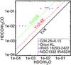 |
Fig. 17 Diagram of HDO/H2O vs. HDCO/H2CO. Data are taken from Table 7. |
| In the text | |
|
Fig. A.1 Original and modified molecular density profiles. The black line shows the original molecular density profile. Different colors indicate different molecular density profiles of models SH1 to SH6. |
| In the text | |
|
Fig. A.2 Comparison of the observed spectra with the results of 6 different shell models (Fig. A.1). Different colors indicate the simulated lines of models SH1 to SH6. The observed and simulated spectra at 241 GHz are very similar to the spectra at 225 GHz; therefore, only the spectra at 225 GHz are plotted here. |
| In the text | |
|
Fig. A.3 Comparison of the density profile of the three different modified models (blue, green, and pink) and original Rolffs’ model (red). |
| In the text | |
|
Fig. A.4 Radial profiles of the continuum emission at 225 (SMA), 241 (SMA), 356 (LABOCA, Rolffs et al. 2011), and 848 GHz (SABOCA, Wyrowski et al., in prep.) The modified models are overlaid in different colors (model D1 – green, D2 – dark-blue, and D3 – purple). The red and grey lines are reproduced profiles from the original Rolffs’ and Nomura’s models. The beam is shown as a orange dashed Gaussian. The errorbars represent only the deviation from a circular shape. |
| In the text | |
|
Fig. A.5 Comparison of the observed spectra with the best-fit results of 3 different models with modified density profiles (Fig. A.3). The red lines are the best-fit model of the original Rolffs profile. The observed and simulated spectra at 241 GHz are very similar to those at 225 GHz; therefore, only the spectra at 225 GHz are plotted here. |
| In the text | |
|
Fig. A.6 Comparison of the temperature profiles of the four different modified models (blue, green, light blue and purple) and the one of the original Rolffs model (red). |
| In the text | |
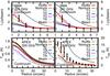 |
Fig. A.7 Same as Fig. A.4, but for the modified temperature models. |
| In the text | |
|
Fig. A.8 Comparison of the observed spectra and those reproduced with the fixed fractional abundances of models T1 to T4. The red lines are the best-fit model with the Rolffs original density profile. |
| In the text | |
Current usage metrics show cumulative count of Article Views (full-text article views including HTML views, PDF and ePub downloads, according to the available data) and Abstracts Views on Vision4Press platform.
Data correspond to usage on the plateform after 2015. The current usage metrics is available 48-96 hours after online publication and is updated daily on week days.
Initial download of the metrics may take a while.