| Issue |
A&A
Volume 658, February 2022
|
|
|---|---|---|
| Article Number | A193 | |
| Number of page(s) | 19 | |
| Section | Interstellar and circumstellar matter | |
| DOI | https://doi.org/10.1051/0004-6361/202140577 | |
| Published online | 24 February 2022 | |
SOFIA/GREAT observations of OD and OH rotational lines towards high-mass star forming regions
1
Laboratoire d’astrophysique de Bordeaux, Univ. Bordeaux, CNRS, B18N, allée Geoffroy Saint-Hilaire,
33615
Pessac,
France
e-mail: This email address is being protected from spambots. You need JavaScript enabled to view it.
2
Max-Planck-Institut für Radioastronomie,
Auf dem Hügel 69,
53121
Bonn,
Germany
3
I. Physikalisches Institut der Universität zu Köln,
Zülpicher Strasse 77,
50937
Köln,
Germany
Received:
16
February
2021
Accepted:
26
November
2021
Abstract
Context. Only recently, OD, the deuterated isotopolog of hydroxyl, OH, has become accessible in the interstellar medium; spectral lines from both species have been observed in the supra-Terahertz and far infrared regime. Studying variations of the OD/OH abundance amongst different types of sources can deliver key information on the formation of water, H2O.
Aims. With observations of rotational lines of OD and OH towards 13 Galactic high-mass star forming regions, we aim to constrain the OD abundance and infer the deuterium fractionation of OH in their molecular envelopes. For the best studied source in our sample, G34.26+0.15, we were able to perform detailed radiative transfer modelling to investigate the OD abundance profile in its inner envelope.
Methods. We used the Stratospheric Observatory for Infrared Astronomy (SOFIA) to observe the 2Π3∕2 J = 5∕2−3∕2 ground-state transition of OD at 1.3 THz (215 μm) and the rotationally excited OH line at 1.84 THz (163 μm). We also used published high-spectral-resolution SOFIA data of the OH ground-state transition at 2.51 THz (119.3 μm).
Results. Absorption from the 2Π3∕2 OD J = 5∕2−3∕2 ground-state transition is prevalent in the dense clumps surrounding active sites of high-mass star formation. Our modelling suggests that part of the absorption arises from the denser inner parts, while the bulk of it as seen with SOFIA originates in the outer, cold layers of the envelope for which our constraints on the molecular abundance suggest a strong enhancement in deuterium fractionation. We find a weak negative correlation between the OD abundance and the bolometric luminosity to mass ratio, an evolutionary indicator, suggesting a slow decrease of OD abundance with time. A comparison with HDO shows a similarly high deuterium fractionation for the two species in the cold envelopes, which is of the order of 0.48% for the best studied source, G34.26+0.15.
Conclusions. Our results are consistent with chemical models that favour rapid exchange reactions to form OD in the dense cold gas. Constraints on the OD/OH ratio in the inner envelope could further elucidate the water and oxygen chemistry near young high-mass stars.
Key words: stars: formation / HII regions / ISM: molecules / submillimeter: ISM
© T. Csengeri et al. 2022
 Open Access article, published by EDP Sciences, under the terms of the Creative Commons Attribution License (https://creativecommons.org/licenses/by/4.0), which permits unrestricted use, distribution, and reproduction in any medium, provided the original work is properly cited.
1 Introduction
The hydroxyl radical, OH, is a key molecule to our understanding of interstellar chemistry, in particular to constrain chemical pathways leading to the formation of water, a prime molecule of interest for star- and planet formation (for a review see van Dishoeck et al. 2013). Tracing its deuterated form, OD, promises to place additional constraints on formation routes through the establishment of the deuterium fractionation within protostellar envelopes.
The OH radical has been observed in various environments, first through its radio lines corresponding to transitions between rotational energy levels split by the magnetic hyperfine structure (hfs) of the molecule (see e.g. Weinreb et al. 1963 and Weaver & Williams 1964). Cesaroni & Walmsley (1991) discussed observations of multiple hfs transitions and modelled their excitation, which generally is not governed by local thermodynamic equilibrium (LTE). As shown in their energy level diagrams in Fig. 1, the rotational transitions of OH (and those of OD) lie in the supra-THz regime at >1.3 THz and are only accessible from space and with airborne facilities. The first observations of rotational transitions of OH were performed with the Kuiper Airborne Observatory (Storey et al. 1981; Melnick et al. 1987; Betz & Boreiko 1989) and have been followed by the Infrared Space Observatory (Ceccarelli et al. 1998; Giannini et al. 2001; Nisini et al. 2002), all with modest spectral resolution of tens of km s−1. Only recently, observations of rotational transitions of OH have become accessible at higher spectral resolution with the Heterodyne Instrument for the Far-Infrared aboard Herschel (HIFI; Wampfler et al. 2011, 2013) and the German Receiver for Astronomy at Terahertz Frequencies (GREAT) on SOFIA (Csengeri et al. 2012; Wiesemeyer et al. 2012, 2016; Parise et al. 2012). With this receiver, the ground-state rotational line of its deuterated form, OD, was first detected in absorption towards the envelope of the low-mass protostar IRAS 16293−2422 (Parise et al. 2012).
The OH molecule is a key component in the water chemistry pathway. At low temperatures, both species are intimately related, forming in the gas phase via dissociative recombination of the oxonium ion, H3O+ (Neau et al. 2000; Jensen et al. 2000 and references therein). The latter is synthesised through a sequence of molecular hydrogen abstraction reactions (Dalgarno 1994) and is therefore sensitive to the molecular gas fraction. At high temperatures, OH forms through gas phase reactions from the reaction between atomic oxygen and hydrogen molecules, and through successive hydrogenation is converted into water (Charnley 1997; Harada et al. 2010; van Dishoeck et al. 2014). The reaction of OH + H2 ⇌ H2O + H, which is endothermic by 920 K, is sensitive to the ratio of atomic O and H and thus depends strongly on the local conditions, such as the temperature and UV field. OH is also a by-product of H2O photodissociation, making it a sensitive tracer of the radiation field. This, for example, results in the high OH abundances in the densemolecular envelopes of (ultra)compact HII regions (see e.g. Cesaroni & Walmsley 1991; Csengeri et al. 2012). The formation of OH is also dependent on the cosmic ray ionisation rate and the gas density (Wakelam et al. 2010).
Since OH is chemically linked to the formation of water, to measure the OD/OH ratio in star forming regions presents a promising tool to constrain the formation conditions of water. For the first time, we can observationally constrain this ratio, which is expected to probe the chemical formation pathway for these molecules, as deuterium enhancement (i.e. fractionation) is strongly dependent on the chemical route and its formation conditions (e.g. Croswell & Dalgarno 1985; Roberts & Herbst 2002). Since deuterium is of solely primordial origin (Peebles 1966) and is destroyed in stars through fusion to 3He, a better understanding of its fractionation into OD may ultimately help to set constraints on star formation history.
Making use of the capabilities of the SOFIA/GREAT receiver, we investigated the OD/OH ratio towards a sample of 13 Galactic high-mass, star forming regions. Most of our targets are well-known Galactic massive star-forming regions subject to extensive studies (e.g. van der Tak et al. 2006; Wyrowski et al. 2016; König et al. 2017). They cover a range of evolutionary stages, characterized by clumps hosting embedded ultra-compact HII (UCHII) regions and internally heated hot molecular cores, as well as quiescent massive sources. Our classification of the evolutionary stage of the sample is based on the type of embedded sources associated with them. In short, sources associated with compact radio emission from the CORNISH catalogue Purcell et al. (2013) or Walsh et al. (1998) are listed as UCHII regions. Parallel or already prior to this stage clumps appear as infrared-bright luminous sources due to the internally heated gas, often referred to as infrared bright massive clumps (cf. Csengeri et al. 2016; König et al. 2017). This stage is frequently characterised by rich molecular emission mainly originating from complex organic molecules leading to the emergence of hot cores. Many of our targets are well-characterised rich molecular hot cores that we also indicated in Table 1. The two quiescent sources G23.21–0.3 and G34.41+0.2 lack bright emission at mid-infrared wavelengths and are likely to correspond to the earliest stages in the evolutionary sequence leading to high-mass star and cluster formation. For this sample of sources, this classification approach is in agreement with a classification based on the physical properties of the clumps, using their bolometric luminosity (Lbol) and clump mass (cf. König et al. 2017). We list the sources and give a summary of the observed lines and transitions in Table 1.
This paper is organised as follows. In Sect. 2, we introduce the observed data and the used datasets, and in Sect. 3 we present our observational results. We perform a detailed non-local thermodynamic equilibrium (non-LTE) radiative transfer modelling in Sect. 4 and discuss our results in Sect. 5.
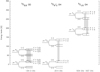 |
Fig. 1 Ground state and first excited energy levels of the 2Π3∕2 OD, OH, and 2Π1∕2 OH states. Greyarrows mark the transitions discussed in this study, whose frequencies are given at the bottom. The zero level of the energy scale refers to the vibrational ground states (2658 and 1941 K for OH and OD, respectively). |
2 Observations and data reduction
2.1 SOFIA/GREAT observations
We used the high spectral resolution GREAT receiver1 (Heyminck et al. 2012; Risacher et al. 2016) on board the Stratospheric Observatory for Infrared Astronomy (SOFIA; Young et al. 2012) to observe rotational transitions of the OD and OH lines. Our primary focus was the 2 Π3∕2 ground-state (J = 5∕2−3∕2) transition of2OD at 1391.5 GHz, which was complemented towards the majority of our sample by observations of the 2 Π1∕2 excited-state (J = 3∕2−1∕2) Λ-doublet transitions of OH at 1834.7 (163.4 μm) and 1837.8 GHz (163.1 μm), respectively.
The observations were carried out as part of GREAT consortium guaranteed observing time in the observatory’s Cycle 1, and Cycle 4 programmes. Best spectroscopic baselines were obtained by means of the chop-and-nod procedure (double-beam switching), with chop amplitudes of 30′′ –60′′, operated at a frequency of 1 Hz. Owing to the double-sideband reception of GREAT, the selection of the sideband and intermediate frequency was optimized with regard to the atmospheric transmission (so as to avoid ozone features) and to receiver sensitivity. In Cycle 1 for OD, the signal was recorded at 1391.5 GHz using the L1 band of GREAT tuned in the upper side-band, and for the 2 Π1∕2 excited-state OH line using the L2 band at 1837.8 GHz tuned in the upper side-band. The 2.5 GHz wide intermediate frequency band was tuned to 1.7 GHz offset, allowing us to simultaneously cover the 1834.7 GHz Λ-doublet pair in the image band. In Cycle 4, the 2Π1∕2 excited-state OH line was observed using the GREAT low frequency array module (LFA) array and was also tuned to 1837.8 GHz in the upper side-band. We also recorded the 2 Π3∕2 ground-state 18OH line at 2494.7 GHz towards G34.26+0.15 and G351.58−0.4 using the Ma channel of GREAT (Heyminck et al. 2012) in Cycle 1 in July 2013. The receiver was tuned to 2494.420 GHz in the upper side band.
We used the extended fast Fourier transform spectrometers (XFFTS) as backends with 2.5 GHz bandwidth and 76 kHz spectral resolution in Cycle 1, and the FFTS4G in Cycle 4 providing a 4 GHz bandwidth. The median single-sideband system temperature was ~1200 K at 1391.5 GHz, and ~1600 K at 1834.7 GHz (Rayleigh-Jeans equivalent antenna temperatures at systemic velocity). The pointing was established with the optical guide cameras providing an accuracy of 2–3′′, and linked to the instrument reference frame by peaking up on Mars or Jupiter right after each reinstallation of the GREAT receiver system. The observed lines for each source are listed in Table 1, and a detailed summary of the observed transitions is listed in Table 2.
The data were calibrated using standard procedures based on the KOSMA/GREAT calibrator (Guan et al. 2012), and for the data analysis we used the GILDAS2 software. The transmission correction was based on the AM atmosphere model3, scaling the measured total power by a forward efficiency of 97%. We fine-tuned the correction for the ozone features by scaling their column densities in AM by factors of order unity until they disappeared against the continuum signal. The data was then converted to a Rayleigh-Jeans equivalent main-beam brightness temperature (Tmb,RJ) scale using a beam efficiency of 67% at both frequencies for Cycle 1, and of 70% for the 1837.8 GHz observations in Cycle 4. For the 18OH line, we used a beam efficiency of 70%.
For the OD line, we obtained the continuum emission by means of a dedicated double-sideband calibration. The Λ-doublet pair of the 2Π1∕2 excited-state OH lines originates from different sidebands and was therefore calibrated considering the different atmospheric transmission in the image and signal bands. The spectra from the signal and image band calibration were then stitched together at an emission-free velocity to obtain a composite spectrum with the respective atmospheric calibration for the spectral features from both the signal and image band.
For both the 2Π3∕2 OD (J = 5/2–3/2) and the 2Π3∕2 OH (J = 3/2–1/2) lines, the spectra were first summed up to define windows excluding the lines for the baseline fitting. Then we used a polynomial baseline to fit the continuum emission and subtracted the fitted continuum from each scan individually. The spectra were then averaged with noise weighting and were smoothed to ~0.65 and 0.75 km s−1 at 1391.5 and 1837.8 GHz, respectively. We reach an average noise of 84 and 87 mK for these velocity resolutions. The half-power beam width (HPBW) is ~20′′ at 1391.5 GHz, 16′′ at 1837.8 GHz. The same procedure has been applied for the 18OH line; however, the baseline variations needed a more careful treatment for G34.26+0.15 due to instrumental effects (see Appendix C).
Target sources and observed species.
2.2 Archival SOFIA data
To put better constraints on the origin of the emission, we used data resulting from SOFIA observations of the 2 Π3∕2, J = 5∕2−3∕2 OH rotational ground-state transition at 2514 GHz from Wiesemeyer et al. (2012, 2016). The observational setup and data reduction steps are similar to those described above. The final spectra were smoothed to 0.9 km s−1 velocity resolution and have a median noise level of ~0.3 K. The HPBW is 12′′ at 2514 GHz.
2.3 Archival Herschel data
To compare the OD and HDO line profiles, we used spectra of the HDO (JK,A = 11,1−00,0) line at 893.6 GHz (Coutens et al. 2014) observed by the Herschel/HIFI instrument, where available. In addition to this, to assist the detailed modelling of G34.26+0.15, we also used a spectrum of the p-H O (11,1−00,0) line at 1101.698 GHz (Flagey et al. 2013). These observations were made in the framework of the Probing Interstellar Molecules with Absorption Line Studies (PRISMAS) Guaranteed Time Key programme (Gerin et al. 2010; Neufeld et al. 2010). PRISMAS observations employed a dual-beam-switching pointed observing mode with a reference position of ~3′ from the source. We obtained the level 2.5 data products from the Herschel Science Archive and processed the data with the IRAM/GILDAS software. We averaged the horizontal and vertical polarisations and summed up the spectra from the three different local oscillator (LO) tunings that have been used to identify line contamination from the image band. We fitted the spectral baseline over a narrow velocity range around the rest velocities (vlsr) of the sources and assumed a sideband gain ratio of unity to correct for the double-sideband receiver. We then used a beam efficiency of 74% (Roelfsema et al. 2012) to convert the spectra to a main beam brightness temperature scale.
For G327.29−0.6, we used the HDO (JK,A = 11,1−00,0) line at 893.6 GHz from the WISH (van Dishoeck et al. 2021) programme also observed with the Herschel/HIFI instrument. The data were processed in the same way as above, with the exception that in this case a single frequency setup was used to cover the line.
Molecules and their transitions.
2.4 Archival APEX data
Towards the source G351.58−0.4, the complementary data for the HDO (JK,A = 11,1−00,0) line at 893.6 GHz were observed with the Atacama Pathfinder Experiment Telescope (APEX, Güsten et al. 2006) using the CHAMP+ receiver (Liu 2017).
3 Results
3.1 The OD 2Π3∕2 (J = 5/2 – 3/2) transition
3.1.1 Detection rates
As an example, in Fig. 2 we show the line-to-continuum ratio spectrum (Tl ∕Tc) of the OD 2 Π3∕2 ground-state (J = 5∕2−3∕2) transition at 1391.5 GHz for the quiescent source G23.21-0.3. Spectra for the rest of our sources are shown in Fig. 3. The lines typically exhibit a Gaussian profile that is a blend of the six hfs components of the Λ-doublet transition spanning a velocity range of ~4.2 km s−1 (see also Table 2).
The OD line is detected towards nine of the 13 targets (69%) on the 3.5−22σ level. In many cases, it appears as a strong and narrow absorption feature. We first fitted the spectra with a single or a two-component Gaussian to extract the line parameters and evaluate the detection rate. The fitted line parameters are summarised in Table 3, which also includes the measured continuum emission near the OD line frequency accounting for the double-sideband reception of the signal. Among the non-detections, some sources may show a weak feature close to our signal-to-noise criterion; for example, towards W33A an absorption feature around 2σrms is observed close to the expected LSR velocity (vlsr). In addition, towards W28A the features around the expected vlsr could also be consistent with a weak and broad absorption component and also a line in emission at the 2σrms level. The line profiles of these components would resemble those of the 2 Π3∕2 OH line towards this source analysed in Leurini et al. (2015), although we caution that in our data the baseline quality for this source is inferior to that of the other sources.
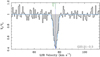 |
Fig. 2 Example of the OD 2Π3∕2 ground-state(J = 5∕2−3∕2) absorption towards the quiescent source G23.21-0.3. The spectra are normalised to the (single side-band) continuum level, and thus show the line to continuum ratio. The rest frequency is set to the strongest hyperfine transition, F = 7/2−–5/2+, at 1391494.70 MHz. The blue dotted line marks the systemic LSR velocity of the source, and the grey dotted line shows the value of1. The blue line shows a single component Gaussian fit to the spectrum. The positions and the relative strength of the hyperfine components are shown in green. |
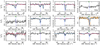 |
Fig. 3 Overview of the OD 2Π3∕2 ground-state(J = 5∕2−3∕2) transition towards the sample. The spectra are normalised to the continuum level and thus show the line-to-continuum ratio. The rest frequency is set to the strongest hyperfine transition, F=7/2−−5∕2+, at 1391494.70 MHz. The vertical blue dotted line marks the systemic LSR velocity of the source (Table 1), horizontal grey dotted line shows the intensity ratio of 1. The light blue line shows a single or a two-component Gaussian fit to the spectrum. The positions and the relative strength of the hyperfine components are shown in green. The red spectra correspond to the HDO (JK,A = 11,1−00,0) line at 893.6GHz from Herschel/HIFI, the orange spectrum shows the same line observed with the APEX telescope. The source name is labelled in the lower right corner of each panel. |
3.1.2 The velocity components of OD absorption
In Figs. 2 and 3, we show the vlsr of the sources from Table 1. The OD 2Π3∕2 (J = 5∕2−3∕2) absorption is typically redshifted compared to the source’s vlsr, which is clearly the case for G34.26+0.15, G351.58–0.4, G10.47+0.03 and W31C, corresponding to 44% of the detections. For these sources, the HDO (JK,A=11,1−00,0) line is also seen similarly redshifted, as well as the NH3 (J = 32+−22−) transition from Wyrowski et al. (2016). The rest velocity at the peak of the absorption is on average ~1.5 km s−1 redshifted for both the OD 2Π3∕2 (J = 5∕2−3∕2) and NH3 (J = 32+−22−) lines.
The OD2Π3∕2 (J = 5∕2−3∕2) absorption feature coincides well with the source systemic velocity for G35.20–0.7, W51e2 and G327.29–0.6, while the NH3 (J = 32+−22−) line is detected as redshifted by Wyrowski et al. (2016). Considering the errors of the fit, which are larger by several factors for the OD line compared to the NH3 line, we find that the vlsr of OD and NH3 are also consistent for these sources.
The OD2Π3∕2 (J = 5∕2−3∕2) absorption is seen blueshifted as comparedto the source’s vlsr towards W49N, often interpreted as a P-Cygni profile due to expanding gas. The same kinematic feature has already been noted by Wyrowski et al. (2016) using the NH3 (J = 32+−22−) line, and it is likely related to the expanding shell structure of this source (Peng et al. 2010). The OD 2 Π3∕2 (J = 5∕2−3∕2) absorption seen towards W49N needs to be fitted with two velocity components; one corresponds to the typically observed narrow absorption feature at the systemic velocity like for the other sources, while the other absorption feature is seen over a broad velocity range of Δv = 11 km s−1. This could be explained if it was associated with outflowing gas at lower velocities than the source’s vlsr.
We detect and resolve two velocity components in absorption towards W51e2, one at the vlsr of the main cloud, and a second component associated with the more diffuse foreground cloud unrelated to W51 Main at ~70 km s−1 (Mookerjea et al. 2014). This is surprising because this gas has been considered to originate from a layer of diffuse gas in front of the W51 Main complex, unrelated to its star formation activity and should have a much lower column density.
It is clear that OD is predominantly found towards massive envelopes of star forming regions in various evolutionary stages. However, considering its detection both in the (presumably) more diffuse medium of the 70 km s−1 component of W51e2 and in outflowing gas from W49N, it appears that it could also be present in sources that have different physical conditions.
3.1.3 The velocity structure of the line
Due to the hyperfine structure of the line, the Gaussian fit overestimates the velocity dispersion. Therefore, we also fit the spectra using the GILDAS/CLASS HFS fitting tool that takes into account the hfs splitting and is based on the assumption that the hfs components have the same excitation temperature. This fit constrains the vlsr and the line width (Δv) relatively well; however, the line opacity (τ) is poorly constrained due to the blending of the components causing large errors in the opacity estimate. To overcome this, we used the line opacity estimated from the line-to-continuum ratio discussed in Sect. 3.1.4 and fixed this value for the HFS fit. The values obtained this way are reported in Table 3.
Comparing the results of the HFS fit to those of a simple Gaussian fit, the HFS fitting reveals that the blending of the six hfs components broadens the line widths considerably, typically by up to a factor of two compared to a simple Gaussian fit to the blended features. In general, the OD absorption is a typically narrow feature with a line width, Δv, between 2.2 and 11.1 km s−1, a mean of 4.2, and a median of 3.2 km s−1. The broadest component is detected towards W49N, and it is likely associated with the outflowing material that is also seen in the 2 Π3∕2 excited OH line (Sect. 3.2). The emission component seen towards W31C is somewhat broader or blueshifted than the absorption component, suggesting either a higher level of turbulent broadening compared to the absorption feature or a different velocity component. This blueshifted component at approximately − 8 km s−1 has also been seen in the o-NH3 (J = 20−10) line at 1214.9 GHz (Persson et al. 2010).
The line width from the OD absorption line is, on average, 4.9 km s−1 with a median of 3.6 km s−1. This is considerably narrower than that of the C17O (J = 3−2) line from Giannetti et al. (2014), which is found to be, on average, 5.7 km s−1 (with a median of 5.8 km s−1). The dispersion on the line-width estimates from the C17O (J = 3−2) line exhibit, however, a considerably smaller dispersion of1.7 km s−1, while the OD line widths have a standard deviation of 3 km s−1 over the sample. This suggests that the OD 2Π3∕2 (J = 5∕2−3∕2) line tends to trace a somewhat more quiescent gas compared to that of the C17O (J = 3−2) line.
Fitresults and gas parameters estimated from the 2Π3∕2 OD J=5/2–3/2 line.
3.1.4 OD column density
The OD 2Π3∕2 (J = 5∕2−3∕2) line is detected in absorption towards all sources, and an emission component is only seen towards W31C with a 3.5 σrms detection measured over the peak brightness temperature of the line. In contrast to the low-mass protostar, IRAS 16293−2422 (Parise et al. 2012), the OD absorption towards massive Galactic star forming regions does not appear to be highly saturated; instead, it is typically optically thin. The deepest absorption with Tl ∕Tc ratios of 0.6 and 0.7 is seen towards G23.21−0.3 and G351.58−0.4, respectively.
The deepest absorption together with the smallest line-widths are observed towards sources that are typically the youngest, like G23.21−0.3, or that are still dominated by a massive, but relatively cold envelope, such as G351.58−0.4, G327.29−0.6. The total optical depth is τtot = ∑iτi, where i corresponds to the hfs component of the line, and we estimated it using the formula 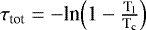 , where Tl corresponds to the main beam brightness temperature of the line and Tc is the continuum temperature accounting for the double-sideband reception of the signal. We find that the values for τtot range between 0.04 and 1.29, with a median of 0.15 and a mean of 0.34, implying that the absorption is typically optically thin. The largest optical depths (τtot) measured towards G351.58−0.4 and G23.21−0.3 are 1.29 and0.89, respectively. The smallest values are seen towards the broad absorption component of W49N, and the 70 km s−1 diffuse cloud component of W51e2.
Adopting the collisional rate coefficients of OH also for OD (see Sect. 4), we find that the 2 Π3∕2 OD J =5∕2−3∕2 line has a very high critical density, ncrit of > 108 cm−3. Such a highvolume density is unlikely to be present in the gas in which the OD absorption originates. Therefore, LTE conditions are unlikely to apply. Moreover, the upper level energy (hν∕k = 67 K) largely exceeds the temperature of the cosmic microwave background. Therefore, it is safe to assume that for all sources the vast majority of OD molecules are in the rotational ground state. The total column density of the molecule can then be estimated as (e.g. Comito et al. 2003)  , where νi is the transition frequency and Aul, i the Einstein-coefficient of transition i. Δvi is the equivalent width of the line, which relates to its full width at half maximum ΔvFWHM reported in Table 4 via
  . gl, i and gu, i are the lower and upper state degeneracies, and τi is the optical depth at the line centre of the i hfs component. The summation extends over the observed Λ-doublet component and applies a correction for the OD population in the other one so as to obtain Ntot. We find values between 3.9 × 10¹² and 6.9 × 1013 cm−2, where the lowest values are typically measured towards the more evolved sources hosting UCHII regions, and the highest values towards the sources that are dominated by a significant amount of cold dust corresponding to quiescent regions and hot cores. This conclusion is fairly robust against our assumption of a complete ground-state population: we repeated the analysis assuming an excitation temperature of 20 K instead, and the deviation in the deduced Ntot is within or close to our fit errors.
Fitresults of the 2Π1∕2 OH J = 3/2–1/2 line.
3.2 The 2Π1∕2 OH (J = 3/2–1/2) transition
We observed the rotationally excited 2Π1∕2 OH (J = 3/2−1/2) transition at 1834.7 GHz towards ten sources of the sample, and show both Λ-doublet transitions in Fig. 4. Two sources without an OD detection, W51d and G31.41+0.2, as well as the quiescent source, G23.21−0.3, and the UCHII region, W51e2, have not been observed in this line. Furthermore, the excited OH line is not detected towards G351.58−0.4 and G327.29−0.6. Towards W33A, only one of the Λ doublets falls in the band.
The remaining sources show relatively bright emission in the 2 Π1∕2 OH (J = 3/2−1/2) line. The Λ doublets have three hfs components (Table 2), the 1834.7 GHz line has an isolated hfs component separated by 11.5 km s−1, which appears as a distinct feature in the spectra. The largest velocity shift for the other Λ-doublet component at 1837.8 GHz is separated by 1.9 km s−1, so all its three hfs components appear blended in the spectra.
The OH line profiles frequently exhibit a broad velocity component likely associated with outflowing high-velocity gas, which is very pronounced in W49N, W28A, and W33A. Towards G10.47+0.03, the outflow component appears to be in absorption. Previously, outflowing gas has been found in excited OH towards the high-mass star forming region W3 IRS 5, where Wampfler et al. (2011) also detected both the envelope and outflow components. Our previous SOFIA/GREAT observations of this excited OH line did not have a high enough signal-to-noise ratio (S/N) to be sensitive to weaker broad components (Csengeri et al. 2012). Low spectral resolution observations with Herschel similarly suggest that the exited OH line can be frequently associated with emission from the high velocity outflowing gas (cf. Yang et al. 2018). The high-velocity outflowing gas of W28A has been studied in detail, including the OH data shown here, in Leurini et al. (2015).
In addition to the broad velocity component, a narrow component associated with the envelope is always present. Furthermore, the line profiles towards G34.26+0.15 suggest that both the emission and absorption components are present in the excited OH line, similarly to what is seen in other high density gas tracers (cf. Wyrowski et al. 2016). The spectra towards G10.47+0.03 are a mixture of a narrow emission component and a broader absorption component from the outflowing gas, as discussed above. The double-peaked profile towards W49N suggests absorption from lower-excitation gas in the envelope.
Similarly to our previous work in Csengeri et al. (2012), we used the HFS method of CLASS to fit the lines. We did this separately for the Λ doublets in the signal and image side band, respectively, and list the average of these results in Table 4 and display them in Fig. 4. Except for W49N, where three components were needed, typically one narrow and a broader component was sufficient to fit the data. The brightest emission is seen towards sources that appear typically weak in the ground-state OD line.
The average FWHM line width for the 2Π1∕2 OH (J = 3/2−1/2) line is 10.3 km s−1 for all the sample considering the narrowest components, where two velocity components were fitted. This is more than two times larger than that of the OD 2Π3∕2 (J = 5∕2−3∕2) line, where for the sources also observed in the 2Π1∕2 OH (J = 3∕2−1∕2) line we find an average line-width of 3.6 km s−1.
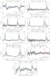 |
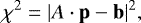
Fig. 4 Overview of OH 2Π1∕2 (J = 3∕2−1∕2) transition towards the sample. The blue dotted line marks the systemic LSR velocity of the source in the signal band. The positions of the hfs lines are labelled in red in the signal and in green in the image band. The HFS fit to the spectra is shown in light blue. The velocity resolution is 0.75 km s−1 for all sources, except for G351.58−0.4, where we show the spectrum at a velocity resolution of 1.5 km s−1. |
Fit parameters from RATRAN modelling of the OH and OD lines.
4 Line modelling with RATRAN
4.1 The physical structure of the envelope
To estimate the abundance distribution of OD and to compare it to that of OH throughout the envelope, we use the non-LTE radiative transfer code RATRAN (Hogerheijde & van der Tak 2000). Following the work of Wyrowski et al. (2016), we constrained the physical structure of the envelope (such as size and the density profile) with the 870 μm dust emission as observed in the APEX Telescope Large Area Survey of the Galaxy (ATLASGAL, Schuller et al. 2009). This implies that we assume that the densities are high enough for the gas and dust to be in thermal equilibrium, which is a reasonable assumption for high-mass protostellar envelopes embedded in massive clumps with high densities. The corresponding parameters of the physical properties are listed in Table 5 for sources with a detection in the ground-state OD line. This allowed us to model six sources.
Our models use a spherical geometry with a power-law profile for the density, n, as a function of radius, r, given by n(r) ~ rαn, and a temperature, T, profile of T(r) ~ r−0.4. The line width is obtained from the C17O (3–2) data for these sources (Giannetti et al. 2014). The velocity gradient through the envelope is constrained by NH3 observations and the models of Wyrowski et al. (2016). The physical structure of the model for G34.26+0.15 is illustrated in Fig. 5, where the bottom panel shows the modelled abundance profiles for OH and OD (see Sect. 4.2). We used the recent collisional rate coefficients from Kłos et al. (2017) for OH for collisions with H2, and adopted these coefficients for OD (see Appendix D for the validity of this approach). We then varied the OH and OD abundances (X(OH) and X(OD)), respectively.
Radiative heating from (high-mass) protostars leads to a radial increase in temperature towards the centre of the envelope (e.g. Wolfire & Cassinelli 1986; Goldreich & Kwan 1974). At low temperatures (< ~20 K), the chemistry is determined by grain surface processes. Triggered by the ignited young stellar object, molecules are desorbed. This greatly changes gas-phase abundances, which are further modified by gas-phase reactions. More importantly, deuterium fractionation of several species is expected to be different in gas-phase reactions compared to grain surface processes (e.g. Roberts & Millar 2007), leading to different molecular abundances in the inner (hot) and outer (cold) regions of envelopes. Since the grain mantles are expected to be mostly composed of water ice, the typical temperature (and thus radius) determining the change of abundances is related to the water evaporation temperature around 100 K (Fraser et al. 2001).
Using 1D, non-LTE radiative transfer modelling, our aim is to estimate the OD abundance in the envelope and to probe what fraction of the OD originates from the hot inner regions and the cold outer envelope. Then, assuming that OH and OD are part of the same gas, we constrained their abundances throughout the envelope and thereby determined the deuterium fractionation by DOD = X(OD)∕X(OH).
For our models, the ground-state 2Π3∕2 OH line seen in absorption should, in principle, provide the best constraint on the OH abundance in the outer envelope. However, as discussed in detail by Wiesemeyer et al. (2016), this line is largely optically thick and is severely blended with absorption from diffuse gas along the line of sight (cf. Wiesemeyer et al. 2012, 2016). Therefore, we can only check whether our models are consistent with these observations. However, towards G34.26+0.15 we obtained archival data from SOFIA covering the 2 Π3∕2 18OH (J = 5∕2−3∕2) ground-state transition at 2494.6950 GHz. This line shows an emission spike at ~50 km s−1 due to a telluricline, which, against strong continuum sources, makes the calibration locally challenging (see Fig. 6 and Wiesemeyer et al. 2012 for details). Nevertheless, we also included the 18OH line in our models assuming an isotopic ratio of 16O/18O = 400 (Wilson 1999).
The 2Π1∕2 OH (J = 3∕2−1∕2) excited-state transition has an upper energy level of 270 K compared to the 67 K of the 2 Π3∕2 OD (J = 5∕2−3∕2) transition, and so it is clearly a more sensitive probe of the warmer inner regions. Nevertheless, we also consider this line to further constrain our models, allowing us to estimate the total OH column density in the envelope.
Summary of RATRAN model parameters and results towards G34.26+0.15.
4.2 G34.26+0.15: Non-LTE modelling of OH, OD, HDO, and H O using RATRAN
4.2.1 Modelling constraints
The source G34.26+0.15 exhibits a profile with redshifted self-absorption in the excited-state OH line, and its source structure is relatively well constrained. Hence, it is for this source that we can perform a more detailed modelling in order to test different OD abundance profiles. The simplest model (A) corresponds to a constant abundance profile through the envelope, while models B, C, and D introduce an abundance jump of OD above a temperature (TJ) of 50, 100, and 200 K, respectively (Fig. 5, bottom panel). OD originating from the warm inner envelope is expected to show up in emission in the blueshifted part of the spectrum, allowing us to constrain the deuterium fractionation in this source for both the inner, warm, and outer cold envelope (appearing in absorption). We list the model parameters, radius (rJ), and temperature(TJ) corresponding to the abundance jump, together with the range of abundances and the modelling results, in Table 6.
For model A, we created a grid of parameters for the OH abundance, X(OH), between 10−10 and 1 × 10⁻⁸. We modelled the deuterium fractionation DOD = X(OD)∕X(OH) between 10−4 and 5 × 10⁻¹. These ranges were sampled by 20 points on a logarithmic scale. For models B and C, we used the result from model A to fix the OH abundance and the deuterium fractionation in the outer envelope, and we varied DODin as listed in Table 6 in an inner radius between rJ = 0′′.2 and 5′′, which translates to physical scales of ~320 and 8000 au, respectively. After performing the calculations with RATRAN, we convolved the modelled spectra with the beam of the telescope at the respective frequencies shown in Table 2 and the hfs structure assuming LTE conditions, meaning we adopted the relative hfs intensities according to their rates of spontaneous emission or absorption4. The models have been compared to the observations and were evaluated by a reduced χ2 method.
For the other molecules shown in Fig. 6, we used the same physical model as for OH and OD, and we used the abundance of Wyrowski et al. (2016) for NH3, and a constant abundance profile for HDO and H O. Since we used the revised distance estimate of 1.4 kpc based on maser parallax measurements (Kurayama et al. 2011) for G34.26+0.15, compared to Coutens et al. (2014), we find that we need to scale their abundances of HDO and H
 O for the outer envelope by factors of 5 and 1.5, respectively, in order to obtain a good fit to the data5.
4.2.2 Constant deuteration profile towards G34.26+0.15
Our first result for G34.26+0.15 is that already a constant OH and OD abundance profile throughout the entire envelope (model A) gives a good fit to all the lines shown in Fig. 6. Our best fit gives an OD abundance, X(OD), of 6.2 × 10⁻¹¹, and we find that an OH abundance, X(OH), of 1.3 × 10⁻⁸ is consistent with the observed 2 Π3∕2 OH ground-state absorption and the 2Π1∕2 excited-state line6. This model corresponds to a constant deuterium fractionation of 4.8 × 10⁻³ throughout the envelope. Our fit reproduces the 1834 GHz Λ-doublet pair of the 2Π1∕2 OH excited line relatively well, although it somewhat over estimates the absorption component. On the other hand, the fit to the 1837 GHz Λ doublet is less good: it underestimates the emission component, and, as for the ground-state-line Λ-doublet pair, it overestimates the absorption component.
Using the same physical model, we also fitted the HDO and p-H O (J = 11,1−00,0) lines with a constant abundance profile of X(HDO) = 1.6 × 10⁻¹¹ and X(H
 O) = 7.8 × 10⁻¹² (corresponding to X(H2O) = 3.1 × 10⁻⁹ assuming an isotopic ratio of 16O/18O = 400). These lines were modelled in detail by Coutens et al. (2014), who adopted a distance of 3.3 kpc for the source, almost two times larger than what we used here based on Wyrowski et al. (2016). It is already interesting that we obtain a good fit to these lines without an abundance jump, suggesting that these observations are not sensitive to the hot inner regions. However, our models require an X(H2O) more than three times lower compared to Coutens et al. (2014) for the outer envelope. In Fig. 6, we also show the observations and the model of the NH3 J = 32,1−22,0 line from Wyrowski et al. (2016) as a comparison. Our results therefore suggest a deuterium fractionation of
  for OD, very similar to that of HDO/H2O of
 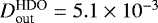 constrained by our modelling here.
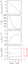 |
Fig. 5 Physical structure of models for G34.26+0.15. Bottom panel shows the OH (red) and OD (grey) abundance variations in the envelope for the different models. For a better visibility, the OD abundance in the inner envelope (X(OD)in) is shifted for the different models. All models test the same abundance range. |
4.3 Impact of evaporation
Due to water ice evaporation, a change in the abundance profile and deuterium fractionation can be expected (see also Coutens et al. 2014 and Sect. 5.3). Therefore, we also tested models introducing a change in deuterium fractionation at a given temperature (TJ). In models B, C, and D we varied the temperature of the abundance jump (TJ = 50, 100, 200 K) and varied the deuterium fractionation in the hot inner regions compared to the outer envelope ( ) in a range of 10−4−5 × 10⁻¹.
In Fig. 7, we show the results of our model B with TJ = 50 K that introduces the abundance jump at a few thousands of au in the envelope, which is comparable to the physical scale of water evaporation found by Coutens et al. (2014). These models show a noticeable change in the blueshifted component of OD seen in emission as a result of the velocity gradient over this source. As we see below, given our sensitivity limit, this is the only model that can put a constraint on the OD column density in the inner regions at rin ~ 11 000 au. Our results suggest that the observations are consistent with a deuterium fractionation in the inner envelope ( ) of up to ~5 × 10⁻³, which would imply that a jump of deuterium fractionation up to a factor of 2 could remain undetected in our observations. However, a strong deuterium enhancement towards the inner regions is clearly excluded by these models. This suggests that the OD abundance in the inner regions cannot be significantly higher than in the outer regions, and thus it does not favour an enhancement in deuterium fractionation in the inner regions compared to the cold envelope. A firmer constraint on the deuterium fractionation towards the innermost regions can only be obtained by observations of higher energy transitions of OD.
We notice that models C and D do not introduce any noticeable change in the model results compared to model A, and additional calculations show that for ‘jump’ temperatures TJ ≥ 60 K, the hot emitting region becomes too small in angular size (≤ 3′′ corresponding to 4800 au) and their emission or absorption is heavily diluted in the SOFIA beam.
We also find that at abundances slightly higher than the values we investigate here, the emission of OH and OD becomes optically thick, and hence it cannot provide a view of the inner regions. Instead, as the higher energy transitions get excited, they should provide a better probe of the inner regions. This fact is somewhat compensated by the velocity structure of the source for G34.26+0.15 and G351.58−0.4 (Fig. 5), allowing us to probe deeper into the envelope due to the accelerated infall, which results in red-shifted velocities closer to the source. For G34.26+0.15 (in contrast to Coutens et al. (2014), whose best fitting models use a temperature of 200 K for anabundance jump), due to the revised distance for this source, our models at the same temperature correspond to a considerably more compact hotter region within 270 au. The Coutens et al. (2014) best fit corresponds to an extent of 1.7′′ (thus 6600 au) in their models, meaning to a value similar to that of our low TJ models.
4.4 Other sources
Above, we discuss the radiative transfer modelling of G34.26+0.15 in detail. For the other sources, we refrained from such a comprehensive modelling in this work due to the lack of a similarly detailed knowledge about the source structure and the lack of sufficient ancillary data in the form of HDO and H O lines. For some sources, though, we were able to rely on the source model of Wyrowski et al. (2016), and we used this as an input for RATRAN to obtain column density estimates primarily for OD and, where available, for OH based on the excited Λ doublets. All these models assume a constant OD abundance profile throughout the envelope similarly to model A for G34.26+0.15.
The parameters of Wyrowski et al. (2016) use the C17O (3–2) measurements from Giannetti et al. (2014) to define the sources’ LSR velocity. They provide a good model for NH3. We adopted the same line width for the OD ground-state absorption, which worked well for all sources, except for G351.58−0.4, for which we find a two times larger line width from the HFS fitting. Our models require this broader line component to provide a good fit to the OD spectrum (see also Appendix A). Similarly, G35.20–0.7 also requires a larger line width (of 2.6 km s−1) than the previous models; however, in this case we find that a constant OH abundance profile does not give a good fit to the excited OH line. The line profiles suggest self-absorption, and while our models reproduce the line profile, they typically underestimate the line intensity, suggesting that OH could be present in a higher abundance towards the warmer inner regions. We suggest that an increased OH column density in the inner envelope could provide a better fit to the observations. The reported OH column density is therefore an upper limit for the outer envelope, and by increasing its value even the excited OH line would appear only in absorption. Due to the limitations of the models for the OH abundance, we obtain the best constraints on the deuterium fractionation (DOD) for G34.26+0.15.The results of these models are summarised in Table 5.
Altogether, the non-LTE radiative transfer modelling gives constraints on X(OD) towards six sources of the sample. These results agree within a factor of 3 with the ones calculated from the absorption features in Sect. 3.1. The largest differences are seen towards G23.21-0.3 and G327.29−0.6, where the modelling gives nearly three times higher OD abundances.
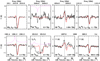 |
Fig. 6 Observed spectra towards G34.25+0.15 are shown in black, and the red line shows the fitted RATRAN model (model A). Dotted line marks the vlsr of the source. Magenta line shows the atmospheric transmission, where the absorption feature in the 18OH spectrum around 50 km s−1 is due to a deliberately uncorrected telluric ozone feature. |
 |
Fig. 7 Results of model B for 2Π3∕2 OD (J = 5/2–3/2) transition of G34.26+0.15 using TJ = 50 K. The different |

5 Discussion
5.1 OD absorption from the cold outer envelope
Absorption from the 2Π3∕2 OD (J = 5∕2−3∕2) ground-state line seems to be prevalent in high-mass star forming regions. It is, however, not exclusively associated with the high column density envelopes, but it is also observed towards various physical components within these regions. It is present in the broad absorption from the outflowing high-velocity gas towards W49N, as well as in the more diffuse gas component seen, for example, towards the 70 km s−1 cloud component around W51e2. In contrast to the low-mass protostar IRAS 16293−2422 (Parise et al. 2012), where the absorption is close to saturation, here the largest optical depths are seen towards the youngest, quiescent sources, and nearby hot cores, where a significant amount of cold dust is still present. These findings are consistent with the chemical models for OD by Croswell & Dalgarno (1985) that predict a high fractionation of OD in the low-density cold gas, while in the dense gas even higher fractionation could be expected depending on the local conditions, such as UV field and fractional ionisation.
Besides the potential outflow and diffuse gas origin, we focus here on the origin of OD within the high-mass protostellar envelopes, that is, the dense gas component. After accounting for the hfs splitting, the line widths we determine are narrow, which is consistent with an origin in the outer envelope where the gas is quiescent. Figure 8 shows a comparison between the measured line-width (Δv) from the OD absorption compared to the estimated total column density. The largest line widths are associated with a more turbulent component of the gas that seems to be less optically thick and have the smallest OD column density in the sample. The largest OD columns show narrow line widths, suggesting an origin from the dense gas of the envelope.
Comparing the vlsr and Δv of the 2 Π3∕2 OD ground-state line with those of the NH3 (J = 32+−22−) absorption at 1.8 THz from Wyrowski et al. (2012, 2016), we notice that the line widths and the line shapes are in general similar (see Appendix B for more details). This further suggests a common origin in the cold absorbing layer of the envelope. Comparing with NH3, in two cases we find a considerably larger line width in the OD line than in the NH3 lines, suggesting a potential contribution from the more inner layers of the envelope. However, there are also other noticeable differences compared to the 1.8 THz NH3 line. In contrast to the narrow OD absorption, NH3 may exhibit velocity components that are not seen in the 2Π3∕2 OD (J = 5∕2−3∕2) line. For example, the broad absorption components seen in NH3 towards the sources G327.29−0.6 and G351.58−0.4 are less pronounced in OD, suggesting either a chemically different environment, or different excitation conditions for this gas component.
The strongest confirmation that the 2Π3∕2 OD (J = 5∕2−3∕2) line originates from the cooler layers of the envelope is given by our detailed radiative transfer modelling of G34.26+0.15. We find that the outer layers of the envelope at typically low temperatures (Td< 80−100 K) and densities below ~ 107 cm−3 are responsible for the absorption feature (Fig. 5). The innermost regions are affected by optical depth effects, the modelled transitions of both OH and OD become optically thick, even before the gas density reaches the critical density (ncr).
With respect to the elemental D/H ratio (~1.5 × 10⁻⁵, e.g. Vidal-Madjar et al. 1983; Linsky 2003), chemical models predict a considerable enhancement of OD in the diffuse gas (Croswell & Dalgarno 1985), where most of the deuterium is expected to be present in atomic form. A significant amount of OD can then be formed through rapid exchange reactions (Roberts et al. 2002); the reaction D + OH ⇌ H + OD is exothermic and has a reaction rate coefficient that is higher at low temperatures (Margitan et al. 1975; Atahan et al. 2005; Wang et al. 2006), leading to a stronger enhancement in OD towards colder gas. The destruction of OD mainly happens through reactions with C+ ions and photodissociation. Our values for the deuterium fractionation in OD, ranging between 4.8 × 10⁻³ and 2.5 × 10⁻², are higher than those predicted for the diffuse gas by these chemical models, and are consistent with a picture where in the dense gas, with less C+ and UV photons the destruction of OD slows down, leading to a stronger deuterium fractionation compared to the diffuse gas.
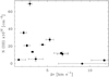 |
Fig. 8 Total column density (N) of the ground-state 2Π3∕2 OD (J = 5∕2−3∕2) line versus the line width (Δv) obtained from the HFS fitting with a fixed total optical depth from the line-to-continuum ratio. |
5.2 Decreasing OD abundance towards the more evolved sources
To investigate the OD abundance variation over our sample of massive clumps in various evolutionary stages, we first used our values for the OD column density, NOD, from Table 3 towards all sources with a detection in the 2 Π3∕2 OD ground-state line. We estimated the H2 column density from the 870 μm beam averaged flux density from the ATLASGAL point source catalogue (Csengeri et al. 2014), because the APEX beam at this frequency is comparable to the beam size of 20′′, corresponding to the OD observations. For the dust temperature (Tdust), we used the values estimated by König et al. (2017) based on fitting the spectral energy distribution (SED) of the dust emission. The Tdust values are found to be between 22.1 and 34.5 K, the temperatures around 30 K are found towards sources hosting embedded UCHII regions. Then, we computed the observationally estimated OD abundance by X(OD) = NOD/NH_2.
We complemented the observationally derived X(OD) estimates (where available) with the results of the radiative transfer modelling (Sect. 4), and hence we can discuss the abundance variations for a sample of nine sources. We find that the highest OD abundances are near the youngest sources of the sample, except for the non-detection towards G34.41+0.2. In particular, G23.21−0.3 and G35.20−0.7 show about an order of magnitude larger abundances than the rest of the sample. Figure 9 shows the distribution of X(OD) as a function of Lbol∕M that we use as a proxy for the evolutionary stage of the clump (see, however, the work of Ma et al. 2013 about Lbol∕M reflecting the mass of the central object). Pearson’s correlation coefficient (ρ) is − 0.56, suggesting a trend of decreasing X(OD) over Lbol∕M. Due to the limited number of sources observed, this correlation is, however, not statistically significant (false alarm probability 16%).
We find that the classification of the sources based on the diagnostic of Lbol∕M does not strictly reflect the evolutionary stage of deeply embedded young stellar objects whose envelopes may just be too compact to impact the Lbol on larger scales. An interesting case is G351.58−0.4, which has a low Lbol∕M, and hence it is expected to be among the younger sources. However, as it shows mid-infrared emission, it has been classified as an infrared bright source in König et al. (2017). Based on radio observations, Culverhouse et al. (2011) find a spectral index consistent with the criteria for UCHII regions from Wood & Churchwell (1989), suggesting that it hosts already formed high-mass star(s). Nevertheless, consistently with its low Lbol∕M, we find a relatively high X(OD), suggesting that the bulk of the gas is chemically young and has not yet been strongly impacted by the star formation process.
Our findings suggest that the OD abundance in the cold dense gas is higher at the onset of the collapse and decreases with time. This is consistent with chemical models predicting that both a higher temperature and stronger radiation field lead to a more efficient destruction of OD. Due to the radiative feedback of newly formed high-mass stars, such conditions occur towards the more advanced evolutionary stages of high-mass star formation. Furthermore, through reactions with O, CO, and C, the OD molecule is destructed in the dense gas; however, these are rather slow processes (Croswell & Dalgarno 1985), suggesting that the lifetime of OD in the cold dense gas is long. The example of G351.58−0.4 suggests that the presence of deeply embedded UCHII regions does not have a strong impact on the OD abundance in the outer layers of the clump, instead the overall Lbol∕M ratio seems more important.
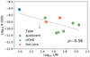 |
Fig. 9 Observed OD abundance (X(OD)) versus Lbol∕M ratio for the entire sample. The colors show the different source types. The grey arrow marks the upper limit estimated for the non-detection of the quiescent source, G34.41. The Pearson correlation coefficient (ρ) is labelled in the figure. |
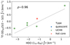 |
Fig. 10 Observed OD and HDO line area measured on the line-to-continuum ratio. The colours show the different source types. |
5.3 OD and HDO: photodissociation and constraints on the water chemistry
The formation and destruction of OH (and OD) are tightly linked to the chemical reaction network of water. Since data for the ground-state HDO line is available for roughly half of the sample, for the more evolved sources, we typically compare and correlate here the observed OD and HDO columns in the cold envelope. From the line shapes shown in Fig. 3, we already notice a resemblance suggesting that the absorptions originate from similar conditions within the envelope. We used the measured area for the 2 Π3∕2 OD (J = 5∕2−3∕2) line from the line-to-continuum ratio (which is directly proportional to the molecular column density in the case of optically thin emission), and perform the same analysis with the HDO ground-state line. Similarly, as in the case for OD, we fitted two velocity components to the HDO line for W49N and W51e2, and we separated the contribution from the outflow and the 70 km s−1 components, respectively. Figure 10 shows the comparison between the OD and HDO absorption from the ground-state transitions. Our results suggest that the OD and HDO column density is correlated; however, we have to note that this result is dominated by the source, G351.58−0.4, which has by far the largest amount of OD and HDO columns. Unfortunately, due to the lack of HDO observations towards a larger number of sources considered young, we cannot conclude whether such a trend holds. However, a tentative correlation between the HDO and OD column would suggest that OD could be a proxy for HDO, and hence H2O, in the outer envelope.
A correlation between OD and HDO might be expected since the formation pathways are tightly linked between OH and H2O. In the cold gas, OH forms together with water as a result of dissociative recombination from H3O+ (Buhr et al. 2010; van Dishoeck et al. 2014). At low temperatures, however, the high water abundance in ices favours a significant contribution from grain surface processes as well (Tielens & Hagen 1982; Roberts & Herbst 2002; Cuppen et al. 2010). On the other hand, at higher temperatures, OH could form through direct reactions between H2 and O if the energy barrier could be overcome (e.g. Elitzur & Watson 1978; Wagner & Graff 1987; van der Tak et al. 2006). A subsequent reaction with H2 then forms followed by H2O. This reaction would essentially convert all OH to H2O, however, the backward reaction proceeds when a strong UV field is present or a high abundance of atomic hydrogen is prevalent. The destruction of OH and H2O is further differentiated by different reaction channels. While H2O is destroyed by an ion-molecule reaction with C+, OH is destroyed by a neutral-neutral reaction with N (Wakelam et al. 2010). More importantly, the equilibrium of the fundamental production and destruction channel of OH + H2 ⇌ H2O + H depends on the local conditions, such as density and temperature. Altogether, this may lead to differences in the OH and H2O abundances throughout the inner envelope. However, when considering the main production channel for H2O, the same reaction for OD + H2 ⇌ HDO + H is likely to be slower (e.g. Thi et al. 2010). Therefore the OD over OH ratio is expected to change once the chemical reaction pathways change in the inner regions. This is expected to lead to a general decrease of HDO/H2O in the hot inner regions, while the OD/OH abundance is expected to increase, and these differences should become more pronounced with time (Coutens et al. 2014).
Based on our radiative transfer modelling of the OH and OD lines, we constrained the deuterium fractionation for OH in the outer envelope. The best estimates are obtained for G34.26+0.15 and G351.58−0.4, which are 4.8 × 10⁻³ and 2.5 × 10⁻², respectively. We obtain an upper limit of the order of 1.5×10⁻² for G35.20−0.7 and a lower limit of 2×10⁻² for G327.29−0.6, which are all sources with low Lbol∕M. Although we do not have a large sample of sources with deuterium fractionation for both OH and H2O, the values collected in Table 5 show that the OD/OH and HDO/H2O values are similar within an order of magnitude. The source G351.58−0.4 shows, however, somewhat larger deuterium fractionation for OD compared to HDO.
While the inner regions are expected to be greatly impacted by the photodissociation of H2O, we cannot put strong constrains on the deuterium fractionation of OD in the hot inner regions here. Our observations exclude, however, a stronger fractionation at regions of a few thousands of au for G34.26+0.15. Observations of higher J transitions of OD could put more constrains on the OD/OH fractionation in the inner region, although large optical depths may prohibit these observations.
6 Conclusions
We report the detection of the 2Π3∕2 OD (J = 5∕2−3∕2) line at 1.3 THz with the SOFIA/GREAT instrument towards a sample of Galactic high-mass star forming regions. We estimate the OD column densities in a range of N(OD) = 4−70 × 1012 cm−2 for these sources, where the highest OD column densities are seen towards the youngest clumps of the sample.
We performed a detailed radiative transfer modelling for one of the best known source of the sample, G34.26+0.15. Our results show that the 2Π3∕2 OD (J = 5∕2−3∕2) absorption originates from the dense and cold outer layers of the envelope. We put constraints on the deuterium fractionation within the inner regions, where, due to sublimation and higher temperatures, gas-phase chemical formation pathways are expected to dominate the chemistry. Although the limits obtained from these models are not stringent, they allow us to exclude a strong enhancement of deuterium fractionation towards the inner envelope.
We estimate the OD molecular abundance in the outer envelope for nine sources of the sample. A correlation with the Lbol∕M ratio - which is used as a proxy for evolutionary stage - shows a tentative slow decrease in the OD abundance with time. This is consistent with chemical models of the cool, dense gas phase, where the main formation of OD proceeds through rapid exchange reactions leading to a strong enhancement of deuterium fractionation. The OD molecule is then destroyed by slow reactions taking place in the outer envelope. Our results suggest that radiation from the deeply embedded heating sources at this stage does not strongly impact the conditions in the envelope.
We find a deuterium fractionation for OD of ~0.5% towards G34.26+0.15 in the outer envelope, which is consistent with estimates from the HDO/H2O ratio. We find a weak correlation between the OD and HDO column in a sample of 6 sources for which ancillary data were available. This suggests that OD could be a proxy for HDO and thus H2O in these sources.
Acknowledgements
We thank the referee for the careful reading of the manuscript and constructive suggestions that improved the paper. Based on observations made with the NASA/DLR Stratospheric Observatory for Infrared Astronomy. SOFIA Science Mission Operations are conducted jointly by the Universities Space Research Association, Inc., under NASA contract NAS2-97001, and the Deutsches SOFIA Institut under DLR contract 50 OK 0901. T.Cs. acknowledges financial support from the French State in the framework of the IdEx Université de Bordeaux Investments for the future Program. The development and operation of GREAT is financed by resources from the participating institutes, by the Deutsche Forschungsgemeinschaft (DFG) within the grant for the Collaborative Research Center 956 as well as by the Federal Ministry of Economics and Energy (BMWI) via the German Space Agency (DLR) under Grants 50 OK 1102, 50 OK 1103 and 50 OK 1104.
Appendix A Model results for G351.58−0.4
In Fig. A.1, we show the results of our RATRAN modelling for G351.58−0.4. As for the other sources, these models assume a constant abundance profile for all species. While the fit for the OD 2 Π3∕2 J = 5/2 – 3/2 transition at 1390.61 GHz is satisfactory, the OH 2Π1∕2 J = 3/2 – 1/2 transition is not well reproduced by this model. As suggested by the NH3 (J = 32+ − 22−) line profile from Wyrowski et al. (2016), the blueshifted component of a broader absorption component is apparent, which also seems to impact the excited-state OH line profiles. Furthermore, our assumption on the constant OH abundance profile may also be inadequate for this source.
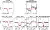 |
Fig. A.1 Same as Fig. 6, but for G351.58−0.4. The observed spectra are shown in black, red line shows the fitted RATRAN model. Dotted line marks the vlsr of the source. The panel for the 2Π3∕2 J=5/2-3/2 transition at 2514 GHz shows the line-to-continuum ratio (Tl∕Tc), all other panels show the line temperature in Kelvins. |
Appendix B Comparison with the NH3 (J = 32+ − 22−) 1.8 THz absorption
We compare the line profiles of the OD 2Π3∕2 J = 5/2 – 3/2 line with the NH3 (J = 32+ − 22−) line in Fig. B.1. For better visibility, the NH3 lines are scaled. We notice that the line profiles are remarkably similar, showing very similar rest velocities. Towards the sources G327.29−0.6 and G351.58−0.4, absorption from a blueshifted broad velocity component, likely due to molecular outflows, is visible in the NH3 line, while it is absent in the ground-state OD line.
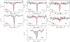 |
Fig. B.1 Comparison between the OD 2Π3∕2 (J = 5∕2 − 3∕2) transition (black) and the NH3 (J = 32+ − 22−) transition (red). |
Appendix C Removal of instrumental artefacts from the 18OH 2Π3∕2 ground-state line
In supra-THz heterodyne spectroscopy, local oscillator (LO) power is precious, and transmission losses in the injection of the generated signal are to be kept at the minimum. The 18OH 2Π3∕2 ground-state line was obtained in 2013, when the LO signals of GREAT (Heyminck et al. 2012) were injected by means of Martin-Pupplet diplexers (e.g. Lesurf 1981). Depending on the tuning, standing waves may arise, causing sinusoidal baselines that are further modulated by the limited frequency passband of the diplexer. Moreover, beyond standing wave features, gain fluctuations can originate in the mixing or subsequent amplification stages. If they are faster than the occurrence of calibration scans, they further deteriorate the baseline quality, especially in observations towards far-infrared, strong continuum sources. These effects together impact the tuning of the Ma band to the 18OH 2Π3∕2 line.
By their nature, these standing waves cannot be removed by a simple Fourier filter, unlike their equivalents occasionally arising between the mixer and the telescope’s secondary mirror. The fitting of high-order polynomial baselines (~10) was found to introduce spurious line profiles at the systemtic velocity and is, likewise, to be avoided. Adjusting sinusoidal waveforms, although numerically somewhat more stable, lacks objectiveness as well. In contrast, differential total power spectra, extracted from the off-source phases of subsequent chop-and-nod sub-scans and typically separated by ~ 1 min, were observed to exhibit similar baseline distortions while being void of the astronomical signal (Higgins et al. 2021, further references therein). In the stable part of the spectral bandpass the aforementioned artefacts are linear in nature, which suggests thenecessity to use a linear combination of such differential off-source total power spectra (hereafter aj, j = 1, 2, ⋯, n) to fit the residual baseline apparent in the averaged on-off spectrum, denoted b. All spectra are represented in an m dimensional vector space, where m is the number of spectral channels considered. For this purpose, we minimised the quantity:
 (C.1)
(C.1)
where the columns of the m × n matrix A are the spectra aj, and where the coefficients of the linear combination minimizing χ2 are denoted as a vector  . Since m > n, the problem to be solved is over-determined; yet, a direct minimisation using normal equations is often numerically unstable, because ambiguous combinations of coefficients p can occur, causing the Jacobian to become singular. However, the solution vector p can be obtained from the easily invertible singular value decomposition (SVD) of matrix A, providing a more stable method to minimise χ2 (e.g. Numerical Recipes, Press et al. 1992). Our baseline fit can then be constructed as
 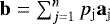 .
.
In practice, we do not directly use the spectra aj, we used smoothed fitting functions instead; this is to avoid excess noise otherwise introduced by the baseline removal. Third order wavelet transforms proved to provide baseline fits with the smallest χ2. Other similarly smoothed variants may yield satisfactory results alike, while higher orders bear the risk of fitting the spectral line as a baseline feature even though the spectra aj do not contain the astronomical signal. As a safeguard against this, we use a weighted fit, modifying Eq. C.1:
 (C.2)
(C.2)
with weights
 (C.3)
(C.3)
centred at υ0 = 60 km s−1. The exact choice of the width Δυ is not critical as long as the putative 18OH absorption line is covered, yet leaving enough spectral baseline on either side (i.e., Δυ = 10 to 15 km s−1). For the computations we use Numerical Recipes routines svdcmp and svbksb to perform the SVD and to calculate p, respectively.
The application of the SVD technique to the baseline removal from the 18OH 2Π3∕2 line is demonstrated in Fig. C.1. After iterative Hanning smoothing to 0.6 km s−1 channel separation, the resulting spectrum features a sensitivity of  mK prior to transmission correction, which equals, within errors, the radiometric noise pertaining to the measured single-sideband system temperature in the relevant part of the bandpass, 6070 K. The obtained spectrum therefore qualifies to define a lower limit to the 16OH∕18OH ratio (Sect. 4 and Fig. 6).
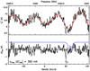 |
Fig. C.1 Spectrum of 18OH 2Π3∕2 before (top) and after (bottom) removal of the SVD derived baseline (red line, top) and transmission correction. The relatively narrow kernel of a telluric O3 line is deliberately left uncorrected. The blue line represents the weight profile used in the χ2 minimisation. |
Appendix D Comparison of RATRAN models with different collisional rate coefficients
In Sect. 4, we used RATRAN to model the OD absorption, and adopted the collisional rate coefficients of OH (Kłos et al. 2017) also for OD. However, recently, collisional rate coefficients for OD with H2 became available (Dagdigian 2021) that also include the hfs splitting. To test the validity of our initial approach, we compared our best fit model for the OD 1391 GHz line (Sect. 4.2) for G34.26+0.15 both using the OH coefficients from Kłos et al. (2017) adapted for OD, and the collisional rate coefficients of OD including the hfs structure from Dagdigian (2021). We show this comparison in Fig. D.1 and see that the difference between the models (red lines) is marginal.
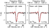 |
Fig. D.1 Comparison of our RATRAN models for the OD 1391 GHz line using the collisional rate coefficients for OD from Dagdigian (2021) (left) and the collisional rate coefficients from OH adapted for OD from Kłos et al. (2017) (right). |
References
- Atahan, S., Alexander, M. H., & Rackham, E. J. 2005, J. Chem. Phys., 123, 204306 [NASA ADS] [CrossRef] [Google Scholar]
- Betz, A. L., & Boreiko, R. T. 1989, ApJ, 346, L101 [NASA ADS] [CrossRef] [Google Scholar]
- Buhr, H., Stützel, J., Mendes, M. B., et al. 2010, Phys. Rev. Lett., 105, 103202 [CrossRef] [Google Scholar]
- Ceccarelli, C., Caux, E., White, G. J., et al. 1998, A&A, 331, 372 [NASA ADS] [Google Scholar]
- Cesaroni, R., & Walmsley, C. M. 1991, A&A, 241, 537 [NASA ADS] [Google Scholar]
- Charnley, S. B. 1997, ApJ, 481, 396 [NASA ADS] [CrossRef] [Google Scholar]
- Comito, C., Schilke, P., Gerin, M., et al. 2003, A&A, 402, 635 [NASA ADS] [CrossRef] [EDP Sciences] [Google Scholar]
- Coutens, A., Vastel, C., Hincelin, U., et al. 2014, MNRAS, 445, 1299 [NASA ADS] [CrossRef] [Google Scholar]
- Croswell, K., & Dalgarno, A. 1985, ApJ, 289, 618 [NASA ADS] [CrossRef] [Google Scholar]
- Csengeri, T., Menten, K. M., Wyrowski, F., et al. 2012, A&A, 542, L8 [NASA ADS] [CrossRef] [EDP Sciences] [Google Scholar]
- Csengeri, T., Urquhart, J. S., Schuller, F., et al. 2014, A&A, 565, A75 [NASA ADS] [CrossRef] [EDP Sciences] [Google Scholar]
- Csengeri, T., Leurini, S., Wyrowski, F., et al. 2016, A&A, 586, A149 [NASA ADS] [CrossRef] [EDP Sciences] [Google Scholar]
- Culverhouse, T., Ade, P., Bock, J., et al. 2011, ApJS, 195, 8 [CrossRef] [Google Scholar]
- Cuppen, H. M., Ioppolo, S., Romanzin, C., & Linnartz, H. 2010, Phys. Chem. Chem. Phys., 12, 12077 [Google Scholar]
- Dagdigian, P. J. 2021, MNRAS, 505, 1987 [CrossRef] [Google Scholar]
- Dalgarno, A. 1994, Adv. Atm. Mol. Opt. Phys., 32, 57 [NASA ADS] [CrossRef] [Google Scholar]
- Elitzur, M., & Watson, W. D. 1978, ApJ, 222, L141 [NASA ADS] [CrossRef] [Google Scholar]
- Flagey, N., Goldsmith, P. F., Lis, D. C., et al. 2013, ApJ, 762, 11 [NASA ADS] [CrossRef] [Google Scholar]
- Fraser, H. J., Collings, M. P., McCoustra, M. R. S., & Williams, D. A. 2001, MNRAS, 327, 1165 [Google Scholar]
- Gerin, M., de Luca, M., Black, J., et al. 2010, A&A, 518, L110 [NASA ADS] [CrossRef] [EDP Sciences] [Google Scholar]
- Giannetti, A., Wyrowski, F., Brand, J., et al. 2014, A&A, 570, A65 [NASA ADS] [CrossRef] [EDP Sciences] [Google Scholar]
- Giannini, T., Nisini, B., & Lorenzetti, D. 2001, ApJ, 555, 40 [Google Scholar]
- Goldreich, P., & Kwan, J. 1974, ApJ, 189, 441 [CrossRef] [Google Scholar]
- Guan, X., Stutzki, J., Graf, U. U., et al. 2012, A&A, 542, L4 [NASA ADS] [CrossRef] [EDP Sciences] [Google Scholar]
- Güsten, R., Nyman, L. Å., Schilke, P., et al. 2006, A&A, 454, L13 [NASA ADS] [CrossRef] [EDP Sciences] [Google Scholar]
- Harada, N., Herbst, E., & Wakelam, V. 2010, ApJ, 721, 1570 [NASA ADS] [CrossRef] [Google Scholar]
- Hatchell, J., Thompson, M. A., Millar, T. J., & MacDonald, G. H. 1998, A&AS, 133, 29 [NASA ADS] [CrossRef] [EDP Sciences] [Google Scholar]
- Heyminck, S., Graf, U. U., Güsten, R., et al. 2012, A&A, 542, L1 [NASA ADS] [CrossRef] [EDP Sciences] [Google Scholar]
- Higgins, R., Kabanovic, S., Pabst, C., et al. 2021, A&A, 652, A77 [NASA ADS] [CrossRef] [EDP Sciences] [Google Scholar]
- Hogerheijde, M. R., & van der Tak, F. F. S. 2000, A&A, 362, 697 [NASA ADS] [Google Scholar]
- Immer, K., Galván-Madrid, R., König, C., Liu, H. B., & Menten, K. M. 2014, A&A, 572, A63 [NASA ADS] [CrossRef] [EDP Sciences] [Google Scholar]
- Jensen, M. J., Bilodeau, R. C., Safvan, C. P., et al. 2000, ApJ, 543, 764 [CrossRef] [Google Scholar]
- Kłos, J., Ma, Q., Dagdigian, P. J., et al. 2017, MNRAS, 471, 4249 [CrossRef] [Google Scholar]
- König, C., Urquhart, J. S., Csengeri, T., et al. 2017, A&A, 599, A139 [Google Scholar]
- Kulczak-Jastrzȩbska, M. 2017, ApJ, 835, 121 [CrossRef] [Google Scholar]
- Kurayama, T., Nakagawa, A., Sawada-Satoh, S., et al. 2011, PASJ, 63, 513 [NASA ADS] [Google Scholar]
- Lesurf, J. C. G. 1981, Infrared Phys., 21, 383 [NASA ADS] [CrossRef] [Google Scholar]
- Leurini, S., Wyrowski, F., Wiesemeyer, H., et al. 2015, A&A, 584, A70 [NASA ADS] [CrossRef] [EDP Sciences] [Google Scholar]
- Linsky, J. L. 2003, Space Sci. Rev., 106, 49 [Google Scholar]
- Liu, F.-C. 2017, PhD thesis, Rheinische Friedrich-Wilhelms-Universität Bonn, Germany [Google Scholar]
- Liu, F.-C., Parise, B., Wyrowski, F., Zhang, Q., & Güsten, R. 2013, A&A, 550, A37 [NASA ADS] [CrossRef] [EDP Sciences] [Google Scholar]
- Ma, B., Tan, J. C., & Barnes, P. J. 2013, ApJ, 779, 79 [Google Scholar]
- Margitan, J. J., Kaufman, F., & Anderson, J. G. 1975, Chem. Phys. Lett., 34, 485 [NASA ADS] [CrossRef] [Google Scholar]
- Melnick, G. J., Genzel, R., & Lugten, J. B. 1987, ApJ, 321, 530 [NASA ADS] [CrossRef] [Google Scholar]
- Mookerjea, B., Vastel, C., Hassel, G. E., et al. 2014, A&A, 566, A61 [NASA ADS] [CrossRef] [EDP Sciences] [Google Scholar]
- Neau, A., Al Khalili, A., Rosén, S., et al. 2000, J. Chem. Phys., 113, 1762 [NASA ADS] [CrossRef] [Google Scholar]
- Neufeld, D. A., Sonnentrucker, P., Phillips, T. G., et al. 2010, A&A, 518, L108 [NASA ADS] [CrossRef] [EDP Sciences] [Google Scholar]
- Nisini, B., Giannini, T., & Lorenzetti, D. 2002, ApJ, 574, 246 [NASA ADS] [CrossRef] [Google Scholar]
- Parise, B., Du, F., Liu, F. C., et al. 2012, A&A, 542, L5 [NASA ADS] [CrossRef] [EDP Sciences] [Google Scholar]
- Peebles, P. J. E. 1966, ApJ, 146, 542 [NASA ADS] [CrossRef] [Google Scholar]
- Peng, T. C., Wyrowski, F., van der Tak, F. F. S., Menten, K. M., & Walmsley, C. M. 2010, A&A, 520, A84 [NASA ADS] [CrossRef] [EDP Sciences] [Google Scholar]
- Persson, C. M., Black, J. H., Cernicharo, J., et al. 2010, A&A, 521, L45 [NASA ADS] [CrossRef] [EDP Sciences] [Google Scholar]
- Pickett, H. M., Poynter, R. L., Cohen, E. A., et al. 1998, J. Quant. Spectr. Rad. Transf., 60, 883 [Google Scholar]
- Press, W. H., Teukolsky, S. A., Vetterling, W. T., & Flannery, B. P. 1992, Numerical Recipes in C. The Art of Scientific Computing (Cambridge: Cambridge University Press) [Google Scholar]
- Purcell, C. R., Hoare, M. G., Cotton, W. D., et al. 2013, ApJS, 205, 1 [Google Scholar]
- Risacher, C., Güsten, R., Stutzki, J., et al. 2016, A&A, 595, A34 [NASA ADS] [CrossRef] [EDP Sciences] [Google Scholar]
- Roberts, H., & Herbst, E. 2002, A&A, 395, 233 [NASA ADS] [CrossRef] [EDP Sciences] [Google Scholar]
- Roberts, H., & Millar, T. J. 2007, A&A, 471, 849 [NASA ADS] [CrossRef] [EDP Sciences] [Google Scholar]
- Roberts, H., Herbst, E., & Millar, T. J. 2002, MNRAS, 336, 283 [NASA ADS] [CrossRef] [Google Scholar]
- Roelfsema, P. R., Helmich, F. P., Teyssier, D., et al. 2012, A&A, 537, A17 [NASA ADS] [CrossRef] [EDP Sciences] [Google Scholar]
- Rolffs, R., Schilke, P., Wyrowski, F., et al. 2011a, A&A, 527, A68 [NASA ADS] [CrossRef] [EDP Sciences] [Google Scholar]
- Rolffs, R., Schilke, P., Zhang, Q., & Zapata, L. 2011b, A&A, 536, A33 [NASA ADS] [CrossRef] [EDP Sciences] [Google Scholar]
- Sánchez-Monge, Á., Cesaroni, R., Beltrán, M. T., et al. 2013, A&A, 552, L10 [NASA ADS] [CrossRef] [EDP Sciences] [Google Scholar]
- Schuller, F., Menten, K. M., Contreras, Y., et al. 2009, A&A, 504, 415 [NASA ADS] [CrossRef] [EDP Sciences] [Google Scholar]
- Storey, J. W. V., Watson, D. M., & Townes, C. H. 1981, ApJ, 244, L27 [NASA ADS] [CrossRef] [Google Scholar]
- Thi, W. F., Woitke, P., & Kamp, I. 2010, MNRAS, 407, 232 [NASA ADS] [CrossRef] [Google Scholar]
- Tielens, A. G. G. M., & Hagen, W. 1982, A&A, 114, 245 [Google Scholar]
- van der Tak, F. F. S., & Menten, K. M. 2005, A&A, 437, 947 [NASA ADS] [CrossRef] [EDP Sciences] [Google Scholar]
- van der Tak, F. F. S., Walmsley, C. M., Herpin, F., & Ceccarelli, C. 2006, A&A, 447, 1011 [NASA ADS] [CrossRef] [EDP Sciences] [Google Scholar]
- van Dishoeck, E. F., Herbst, E., & Neufeld, D. A. 2013, Chem. Rev., 113, 9043 [Google Scholar]
- van Dishoeck, E. F., Bergin, E. A., Lis, D. C., & Lunine, J. I. 2014, in Protostars and Planets VI, eds. H. Beuther, R. S. Klessen, C. P. Dullemond, & T. Henning (Tucson: University of Arizona Press), 835 [Google Scholar]
- van Dishoeck, E. F., Kristensen, L. E., Mottram, J. C., et al. 2021, A&A, 648, A24 [NASA ADS] [CrossRef] [EDP Sciences] [Google Scholar]
- Vidal-Madjar, A., Laurent, C., Gry, C., et al. 1983, A&A, 120, 58 [NASA ADS] [Google Scholar]
- Wagner, A. F., & Graff, M. M. 1987, ApJ, 317, 423 [NASA ADS] [CrossRef] [Google Scholar]
- Wakelam, V., Herbst, E., Le Bourlot, J., et al. 2010, A&A, 517, A21 [NASA ADS] [CrossRef] [EDP Sciences] [Google Scholar]
- Walsh, A. J., Burton, M. G., Hyland, A. R., & Robinson, G. 1998, MNRAS, 301, 640 [Google Scholar]
- Wampfler, S. F., Bruderer, S., Kristensen, L. E., et al. 2011, A&A, 531, L16 [NASA ADS] [CrossRef] [EDP Sciences] [Google Scholar]
- Wampfler, S. F., Bruderer, S., Karska, A., et al. 2013, A&A, 552, A56 [NASA ADS] [CrossRef] [EDP Sciences] [Google Scholar]
- Wang, W., Santos, E., & Brandão, J. 2006, J. Chem. Phys., 124, 074305 [NASA ADS] [CrossRef] [Google Scholar]
- Weaver, H. F., & Williams, D. R. W. 1964, Nature, 201, 380 [CrossRef] [Google Scholar]
- Weinreb,S., Barrett, A. H., Meeks, M. L., & Henry, J. C. 1963, Nature, 200, 829 [NASA ADS] [CrossRef] [Google Scholar]
- Wienen, M., Wyrowski, F., Schuller, F., et al. 2012, A&A, 544, A146 [NASA ADS] [CrossRef] [EDP Sciences] [Google Scholar]
- Wiesemeyer, H., Güsten, R., Heyminck, S., et al. 2012, A&A, 542, L7 [NASA ADS] [CrossRef] [EDP Sciences] [Google Scholar]
- Wiesemeyer, H., Güsten, R., Heyminck, S., et al. 2016, A&A, 585, A76 [NASA ADS] [CrossRef] [EDP Sciences] [Google Scholar]
- Wilson, T. L. 1999, Rep. Prog. Phys., 62, 143 [Google Scholar]
- Wolfire, M. G., & Cassinelli, J. P. 1986, ApJ, 310, 207 [CrossRef] [Google Scholar]
- Wood, D. O. S., & Churchwell, E. 1989, ApJS, 69, 831 [Google Scholar]
- Wyrowski, F., Güsten, R., Menten, K. M., Wiesemeyer, H., & Klein, B. 2012, A&A, 542, L15 [NASA ADS] [CrossRef] [EDP Sciences] [Google Scholar]
- Wyrowski, F., Güsten, R., Menten, K. M., et al. 2016, A&A, 585, A149 [NASA ADS] [CrossRef] [EDP Sciences] [Google Scholar]
- Yang, Y.-L., Green, J. D., Evans, II, N. J., et al. 2018, ApJ, 860, 174 [NASA ADS] [CrossRef] [Google Scholar]
- Young, E. T., Becklin, E. E., Marcum, P. M., et al. 2012, ApJ, 749, L17 [NASA ADS] [CrossRef] [Google Scholar]
GREAT is a development by the MPI für Radioastronomie and KOSMA/Universität zu Köln, in cooperation with the MPI für Sonnensystemforschung and the DLR Institut für Optische Sensorsysteme.
S. Paine, SMA Memo #152, Smithsonian Astrophysical Observatory.
This approximation is not valid for the highly optically thick absorption seen in the ground-state 2 Π3∕2 OH line.
This gives a deuterium fractionation for water vapour in the outer envelope of 5.1 × 10⁻³ instead of 1.5 × 10⁻³ reported in Coutens et al. (2014).
Our model over-predicts the 1.3 THz continuum for the OD 2 Π3∕2 J = 3/2–1/2 transition by 0.65 K (corresponding to 10%), and it under-predicts the continuum by 0.9 K (10%) at 1.8 THz for the OH 2 Π1∕2 J = 5/2–3/2 line. It shows a discrepancy of 3.0 K (corresponding to 50%) for the OH 2 Π3∕2 J = 3/2–1/2 line at 2.5 THz.
All Tables
All Figures
|
Fig. 1 Ground state and first excited energy levels of the 2Π3∕2 OD, OH, and 2Π1∕2 OH states. Greyarrows mark the transitions discussed in this study, whose frequencies are given at the bottom. The zero level of the energy scale refers to the vibrational ground states (2658 and 1941 K for OH and OD, respectively). |
| In the text | |
|
Fig. 2 Example of the OD 2Π3∕2 ground-state(J = 5∕2−3∕2) absorption towards the quiescent source G23.21-0.3. The spectra are normalised to the (single side-band) continuum level, and thus show the line to continuum ratio. The rest frequency is set to the strongest hyperfine transition, F = 7/2−–5/2+, at 1391494.70 MHz. The blue dotted line marks the systemic LSR velocity of the source, and the grey dotted line shows the value of1. The blue line shows a single component Gaussian fit to the spectrum. The positions and the relative strength of the hyperfine components are shown in green. |
| In the text | |
|
Fig. 3 Overview of the OD 2Π3∕2 ground-state(J = 5∕2−3∕2) transition towards the sample. The spectra are normalised to the continuum level and thus show the line-to-continuum ratio. The rest frequency is set to the strongest hyperfine transition, F=7/2−−5∕2+, at 1391494.70 MHz. The vertical blue dotted line marks the systemic LSR velocity of the source (Table 1), horizontal grey dotted line shows the intensity ratio of 1. The light blue line shows a single or a two-component Gaussian fit to the spectrum. The positions and the relative strength of the hyperfine components are shown in green. The red spectra correspond to the HDO (JK,A = 11,1−00,0) line at 893.6GHz from Herschel/HIFI, the orange spectrum shows the same line observed with the APEX telescope. The source name is labelled in the lower right corner of each panel. |
| In the text | |
|
Fig. 4 Overview of OH 2Π1∕2 (J = 3∕2−1∕2) transition towards the sample. The blue dotted line marks the systemic LSR velocity of the source in the signal band. The positions of the hfs lines are labelled in red in the signal and in green in the image band. The HFS fit to the spectra is shown in light blue. The velocity resolution is 0.75 km s−1 for all sources, except for G351.58−0.4, where we show the spectrum at a velocity resolution of 1.5 km s−1. |
| In the text | |
|
Fig. 5 Physical structure of models for G34.26+0.15. Bottom panel shows the OH (red) and OD (grey) abundance variations in the envelope for the different models. For a better visibility, the OD abundance in the inner envelope (X(OD)in) is shifted for the different models. All models test the same abundance range. |
| In the text | |
|
Fig. 6 Observed spectra towards G34.25+0.15 are shown in black, and the red line shows the fitted RATRAN model (model A). Dotted line marks the vlsr of the source. Magenta line shows the atmospheric transmission, where the absorption feature in the 18OH spectrum around 50 km s−1 is due to a deliberately uncorrected telluric ozone feature. |
| In the text | |
|
Fig. 7 Results of model B for 2Π3∕2 OD (J = 5/2–3/2) transition of G34.26+0.15 using TJ = 50 K. The different |
| In the text | |
|
Fig. 8 Total column density (N) of the ground-state 2Π3∕2 OD (J = 5∕2−3∕2) line versus the line width (Δv) obtained from the HFS fitting with a fixed total optical depth from the line-to-continuum ratio. |
| In the text | |
|
Fig. 9 Observed OD abundance (X(OD)) versus Lbol∕M ratio for the entire sample. The colors show the different source types. The grey arrow marks the upper limit estimated for the non-detection of the quiescent source, G34.41. The Pearson correlation coefficient (ρ) is labelled in the figure. |
| In the text | |
|
Fig. 10 Observed OD and HDO line area measured on the line-to-continuum ratio. The colours show the different source types. |
| In the text | |
|
Fig. A.1 Same as Fig. 6, but for G351.58−0.4. The observed spectra are shown in black, red line shows the fitted RATRAN model. Dotted line marks the vlsr of the source. The panel for the 2Π3∕2 J=5/2-3/2 transition at 2514 GHz shows the line-to-continuum ratio (Tl∕Tc), all other panels show the line temperature in Kelvins. |
| In the text | |
|
Fig. B.1 Comparison between the OD 2Π3∕2 (J = 5∕2 − 3∕2) transition (black) and the NH3 (J = 32+ − 22−) transition (red). |
| In the text | |
|
Fig. C.1 Spectrum of 18OH 2Π3∕2 before (top) and after (bottom) removal of the SVD derived baseline (red line, top) and transmission correction. The relatively narrow kernel of a telluric O3 line is deliberately left uncorrected. The blue line represents the weight profile used in the χ2 minimisation. |
| In the text | |
|
Fig. D.1 Comparison of our RATRAN models for the OD 1391 GHz line using the collisional rate coefficients for OD from Dagdigian (2021) (left) and the collisional rate coefficients from OH adapted for OD from Kłos et al. (2017) (right). |
| In the text | |
Current usage metrics show cumulative count of Article Views (full-text article views including HTML views, PDF and ePub downloads, according to the available data) and Abstracts Views on Vision4Press platform.
Data correspond to usage on the plateform after 2015. The current usage metrics is available 48-96 hours after online publication and is updated daily on week days.
Initial download of the metrics may take a while.