| Issue |
A&A
Volume 550, February 2013
|
|
|---|---|---|
| Article Number | A21 | |
| Number of page(s) | 84 | |
| Section | Interstellar and circumstellar matter | |
| DOI | https://doi.org/10.1051/0004-6361/201219890 | |
| Published online | 21 January 2013 | |
Different evolutionary stages in massive star formation
Centimeter continuum and H2O maser emission with ATCA⋆,⋆⋆
1
Osservatorio Astrofisico di Arcetri, INAF, Largo Enrico Fermi 5, 50125
Firenze, Italy
e-mail: This email address is being protected from spambots. You need JavaScript enabled to view it.
2
Istituto di Radioastronomia & Italian ALMA Regional
Centre, via P. Gobetti
101, 40129
Bologna,
Italy
3
Istituto di Fisica dello Spazio Interplanetario, INAF, Area di
Recerca di Tor Vergata, Via Fosso
Cavaliere 100, 00133
Roma,
Italy
4
ESO, Karl
Schwarzschild str. 2, 85748
Garching bei Munchen,
Germany
5
School of Physics, University of New South Wales,
NSW 2052,
Australia
Received:
26
June
2012
Accepted:
30
October
2012
Abstract
Aims. We present Australia Telescope Compact Array (ATCA) observations of the H2O maser line and radio continuum at 18.0 GHz and 22.8 GHz toward a sample of 192 massive star-forming regions containing several clumps already imaged at 1.2 mm. The main aim of this study is to investigate the water maser and centimeter continuum emission (that likely traces thermal free-free emission) in sources at different evolutionary stages, using evolutionary classifications previously published.
Methods. We used the recently comissioned Compact Array Broadband Backend (CABB) at ATCA that obtains images with ~20′′ resolution in the 1.3 cm continuum and H2O maser emission in all targets. For the evolutionary analysis of the sources we used millimeter continuum emission from the literature and the infrared emission from the MSX Point Source Catalog.
Results. We detect centimeter continuum emission in 88% of the observed fields with a typical rms noise level of 0.45 mJy beam-1. Most of the fields show a single radio continuum source, while in 20% of them we identify multiple components. A total of 214 cm continuum sources have been identified, that likely trace optically thin H ii regions, with physical parameters typical of both extended and compact H ii regions. Water maser emission was detected in 41% of the regions, resulting in a total of 85 distinct components. The low angular (~20′′) and spectral (~14 km s-1) resolutions do not allow a proper analysis of the water maser emission, but suffice to investigate its association with the continuum sources. We have also studied the detection rate of H ii regions in the two types of IRAS sources defined in the literature on the basis of the IRAS colors: High and Low. No significant differences are found, with high detection rates (>90%) for both High and Low sources.
Conclusions. We classify the millimeter and infrared sources in our fields in three evolutionary stages following the scheme presented previously: (Type 1) millimeter-only sources, (Type 2) millimeter plus infrared sources, (Type 3) infrared-only sources. We find that H ii regions are mainly associated with Type 2 and Type 3 objects, confirming that these are more evolved than Type 1 sources. The H ii regions associated with Type 3 sources are slightly less dense and larger in size than those associated with Type 2 sources, as expected if the H ii region expands as it evolves, and Type 3 objects are older than Type 2 objects. The maser emission is mostly found to be associated with Type 1 and Type 2 sources, with a higher detection rate toward Type 2, consistent with the results of the literature. Finally, our results on H ii region and H2O maser association with different evolutionary types confirm the evolutionary classification proposed previously.
Key words: stars: formation / stars: massive / Hiiregions / radio continuum: ISM / masers
Appendices are available in electronic form at http://www.aanda.org
Tables 3–5, 7–9 are only, and Table 1 is also available at the CDS via anonymous ftp to cdsarc.u-strasbg.fr (130.79.128.5) or via http://cdsarc.u-strasbg.fr/viz-bin/qcat?J/A+A/550/A21
© ESO, 2013
1. Introduction
The problem of massive star formation (O and B stars with masses ≳8 M⊙) still represents a challenge from both a theoretical and observational point of view. These stars reach the zero-age main sequence (ZAMS) while they still undergo heavy accretion, and their powerful radiation pressure should halt the infalling material, thus inhibiting growth of the stellar mass beyond ~8 M⊙ (e.g., Palla & Stahler 1993). Recently, various studies have proposed a solution to this problem based on non-spherical accretion and high accretion rates (e.g., McKee & Tan 2003; Bonnell et al. 2004; Krumholz et al. 2009; Kuiper et al. 2010). Together with the theoretical efforts, the comprehension of the massive star formation process requires good observational knowledge of the star-forming environment and of the evolutionary steps through which OB star formation occurs.
In 1991, we started a thorough investigation of a sample of luminous IRAS sources, selected on the basis of their far-infrared colors and with the additional constraint of δ > −30° (Palla et al. 1991, 1993). The hypothesis that this sample could contain high-mass young stellar objects (YSOs) in different evolutionary phases has been supported by a large number of observations that we have performed both at low and high angular resolution (Molinari et al. 1996, 1998a,b, 2000, 2002; Brand et al. 2001; Fontani et al. 2004a,b, 2006; Zhang et al. 2001, 2005). We started a similar study in the southern hemisphere, which represents an excellent testbed for these studies thanks to the large number of (massive) star-forming regions that are observable. For this reason, we used the Swedish-ESO Submillimetre Telescope (SEST) to search for CS-line and 1.2 mm continuum emission in a sample of sources with δ < −30° (Fontani et al. 2005; Beltrán et al. 2006). Along the same line, other authors (e.g., Bronfman et al. 1989; Sridharan et al. 2002; Beuther et al. 2002; Fáundez et al. 2004; Hill et al. 2005) have also studied large samples of massive young stellar objects in the millimeter continuum and line emission.
To study a possible evolutionary sequence of the objects, Molinari et al. (2008) performed a detailed analysis of a small subset of our samples from millimeter down to mid-infrared wavelengths. According to these authors, the sources can be divided into three types, in order of increasing age: MM (and MM-S; hereafter Type 1) with dominant millimeter emission and possibly located close to an infrared MSX source, but not coincident with it; IR-P (hereafter Type 2) with both millimeter and infrared emission; and IR-S1/S2 (hereafter Type 3) with only infrared emission but located near a millimeter source. Using a simple model, Molinari et al. (2008) could relate the infrared and millimeter emission to the physical state of the core and explain the distribution of these source types in a mass-luminosity plot in terms of evolution. As illustrated in Fig. 9 of Molinari et al. (2008), Type 1 would correspond to high-mass protostars embedded in dusty clumps, possibly surrounded by infrared emission that could originate from more evolved, nearby lower mass stars (see Faustini et al. 2009), Type 2 would be deeply embedded ZAMS OB stars that still undergo accretion, and Type 3 would be ZAMS OB stars surrounded only by remnants of their parental clumps.
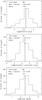 |
Fig. 1 Top: distribution of kinematic distances for the observed fields (see Table 1 for references). Middle: distribution of bolometric luminosities for the fields centered on an IRAS source. Bottom: distribution of the sum of the masses of the millimeter sources within the observed fields (from Beltrán et al. 2006). At the top of each panel we indicate the total number of sources used in the histogram, the mean, the standard deviation, and the median. The vertical dashed lines indicate the median values. |
In this paper, we aim to extend the analysis performed by Molinari et al. (2008) to a larger sample of sources, and add the information of the centimeter continuum emission (likely tracing H ii regions: see e.g., Kurtz et al. 1994; Sánchez-Monge et al. 2008) and H2O masers (which are signposts of the presence of outflows/shocks associated with protostars: e.g., Felli et al. 2007; Moscadelli et al. 2011) to set constraints on the evolutionary scheme. In Sects. 2 and 3 we describe the sample and observations. In Sect. 4 we present the centimeter continuum and maser line results. An analysis of the centimeter continuum sources is presented in Sect. 5, and the evolutionary scenario is discussed in Sect. 6. We end in Sect. 7 with the main conclusions of this work.
Target fields observed by ATCA at 18.0 GHz and 22.8 GHz.
2. Sample
The first step to extend the search for massive YSOs toward the southern hemisphere was to
select a sample of possible candidates from the IRAS Point Source Catalog following the
Palla et al. (1991, 1993) criteria: F60 μm ≥ 100 Jy and
colors satisfying the criteria established by Richards et al. (1987) for compact molecular cores. The sources were divided into two
subsamples based on the IRAS colors: sources with [25−12] > 0.57 and [60−12] > 1.3
were named High (with colors characteristic of sources associated with ultracompact
H ii regions; Wood & Churchwell 1989),
the others were named Low. A sample of 235 IRAS sources, containing 142 Low and 93 High
sources, was observed by Beltrán et al. (2006) at
1.2 mm with the SEST, resulting in a total of 667 millimeter clumps detected. In this paper
we present observations carried out with the Australia Telescope Compact Array (ATCA; see
Sect. 3) toward a large subsample of these millimeter
sources. In total, we observed 192 distinct fields (defined by the full width at half
maximum primary beam of ATCA of ~2 5; see Sect. 3), containing 315 millimeter sources. Out of the total 192 fields, 160 were
centered on an IRAS source (81 Low and 79 High IRAS sources), while the remaining 32 fields
were centered on millimeter clumps (detected with the SEST) located >150′′ from an IRAS
source.
5; see Sect. 3), containing 315 millimeter sources. Out of the total 192 fields, 160 were
centered on an IRAS source (81 Low and 79 High IRAS sources), while the remaining 32 fields
were centered on millimeter clumps (detected with the SEST) located >150′′ from an IRAS
source.
In Fig. 1 we show the distributions of kinematic distances, bolometric luminosities, and masses of the sources observed with ATCA. Note that we only have distance determinations for 189 of the 192 observed fields, most of them obtained from CS-line observations (Fontani et al. 2005; Beltrán et al. 2006, see Table 1). For 96 of these fields there is an ambiguity between near and far distances (see Beltrán et al. 2006). Searching the literature, we were able to solve the ambiguity for 36 fields (using H i line observations; see references in Table 1), for the remaining fields we considered the near distance for the analysis1. The bolometric luminosities were derived only for the 157 fields centered on an IRAS source with distance determination (see middle panel of Fig. 1). Finally, we considered the sum of the masses of the millimeter sources within our observed fields and constructed the distribution of masses. The median values of 4.3 kpc, 2 × 10⁴ L⊙, and 300 M⊙, and the distributions are similar to those obtained for all sources in Beltrán et al. (2006), confirming that our source selection is representative of the whole sample.
3. Observations and data reduction
The 192 selected fields were observed with the ATCA interferometer at Narrabri (Australia) on July 25 and 26, 2009, and October 9 and 10, 2009 (project C1804). In Table 1, we list the observed fields. Column 1 gives the field name, Col. 2 the source type of the IRAS source (High or Low), Col. 3 the kinematic distance adopted, Cols. 4 to 7 give the coordinates of the phase center2 (both in equatorial and galactic systems), Cols. 8 to 13 give the synthesized beams, position angles, and rms noise levels at 18.0 GHz and 22.8 GHz, and Col. 14 indicates the day of observation of the field. Observations were conducted using the recently commissioned Compact Array Broadband Backend (CABB; Wilson et al. 2011), whichi provides a total bandwidth of 4 GHz divided into two sidebands: 2 GHz in the lower sideband (LSB) centered at a frequency of 18.0 GHz, and 2 GHz in the upper sideband (USB) centered at a frequency of 22.8 GHz, covering the H2O (615–523) maser transition at 22.235 GHz (although with low spectral resolution: channel width of 1 MHz, corresponding to ~13.5 km s-1). The array was in the H75 configuration for the four observing runs, resulting in a synthesized beam of ~25′′at 18.0 GHz and ~20′′ at 22.8 GHz.
Observations were conducted in snapshot mode. The typical strategy was to observe each target field for 10 min. This total on-source time was broken up into a series of 3 min snapshots in order to achieve a better coverage of the uv plane. A gain calibrator was observed every 15 min to correct for the phase variations. A total of 14 gain calibrators3 were used for the 192 target observed fields. The absolute flux scale was calibrated daily using PKS B1934−638 as a primary calibrator for all four observing runs. The flux of PKS B1934−638 was assumed to be 1.03 Jy at 20 GHz. Daily bandpass calibration was achieved by observing 0537−441 (with a flux of 8.35 Jy).
The data reduction was made with the MIRIAD software package (Sault et al. 1995). In all cases, data from the antenna located at 6 km from the main array (antenna CA06) were excluded from the data reduction to avoid an increase in the rms noise of the final images. Images of each target field were produced using the CLEAN algorithm with natural weighting. Fields with water maser emission at 22 GHz were self-calibrated. The self-calibration process consisted of identifying the channel with the strongest maser component, self-calibrate it (using the task SELFCAL), and apply the gain solutions to the continuum at 22.8 GHz and 18.0 GHz if both continuum maps improved with the new gain solutions. The mean rms noise is 0.45 mJy beam-1 at 18.0 GHz and 0.40 mJy beam-1 at 22.8 GHz (see Table 1 for the noise in individual fields).
4. Results
4.1. Centimeter continuum emission
In Fig. B.1, we present a panel for each field, showing the centimeter continuum emission at 18.0 GHz (color scale) and 22.8 GHz (contours). In Fig. B.2, we present three panels (in a row) for each field, showing all possible comparisons between maps of the radio continuum emission, the 1.2 mm continuum from SEST (Beltrán et al. 2006), and the 21.8 μm emission from the MSX (Midcourse Space Experiment; Price et al. 1999). We detect centimeter continuum emission above the 5σ level in 169 out of 192 fields, corresponding to a detection rate of 88%. In most of the maps, the centimeter continuum emission comes from a single object, and only a few of them show extended complex emission with multiple peaks. To identify the centimeter sources and derive their properties, we used the following criterion: if the contour at half-maximum of the intensity peak (over 5σ) is closed, we considered it to be an independent source. With this method we identified a total of 214 centimeter continuum sources. There are multiple sources in 38 fields and a single detection (with an angular resolution of ~20′′) in 131 fields. Therefore, in 12% of the 192 observed fields no centimeter continuum emission is detected, in 68% we find a single component, and in 20% of the targets there are multiple sources. In Table 2 we list a summary of the detections in the observed fields, distinguishing between fields that are centered on IRAS sources and fields that are not. We can see that most of the fields with no continuum detection (65%) correspond to fields centered on a millimeter source located far from the IRAS source.
Summary of centimeter continuum detections.
In Table 3, we list all the sources detected and, for completeness, the 23 fields with no
centimeter emission, indicating 5σ upper limits. We give the name of the
region (Col. 1), the number of each centimeter continuum source detected in a field
(Col. 2), the coordinates of the 22.8 GHz detection4
(except where otherwise indicated, in which case the coordinates of the 18.0 GHz source
are reported; Cols. 3 and 4), the peak intensity, integrated flux, observed size and
deconvolved size at 18.0 GHz (Cols. 5 to 8) and at 22.8 GHz (Cols. 9 to 12), and the
association of a water maser with the centimeter source (Col. 12). The angular diameter,
θS, was calculated assuming the sources are Gaussians from
the expression  with FWHP =
2
with FWHP =
2 , where A is the area
inside the polygon corresponding to the contour at half maximum, and HPBW is the
synthesized beam listed in Table 1. For the unresolved sources we considered an upper
limit on the angular diameter of 7′′, i.e., 1/3 of the synthesized beam.
, where A is the area
inside the polygon corresponding to the contour at half maximum, and HPBW is the
synthesized beam listed in Table 1. For the unresolved sources we considered an upper
limit on the angular diameter of 7′′, i.e., 1/3 of the synthesized beam.
In the top panel of Fig. 2, we show the distribution of flux densities for the detected sources. The mean and median values are 47 and 46 mJy at 18.0 GHz, and 40 and 37 mJy at 22.8 GHz. Thus, we are typically measuring fluxes at 22.8 GHz lower than at 18.0 GHz. This can be caused either by the flux density decreases with frequency for the detected sources (as expected in optically thin H ii regions), or by some part of the centimeter emission that is filtered out at shorter wavelengths (as seen by comparing the images in sources like 10184−5748 and 13106−6050).
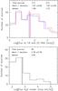 |
Fig. 2 Top: distributions of the flux density of the centimeter continuum sources detected at 18.0 GHz (blue, 212 sources) and 22.8 GHz (red, 213 sources). Note that the number of sources detected at both wavelengths is different, since one source is detected only at 18.0 GHz and two sources are detected only at 22.8 GHz (see Table 3). Bottom: distribution of the integrated flux of the H2O maser emission. The numbers at the top of each panel correspond to the total number of sources, the mean, the standard deviation, and the median values. |
4.2. Water maser emission
Although the main goal of our observations was the study of the centimeter continuum emission, we also observed the H2O maser line at 22.235 GHz. In Table 4, we list the properties of the detected masers: the name of the region, the coordinates, the integrated intensity, and the velocity of the peak of the emission. Owing to the poor spectral resolution (~13.5 km s-1), the maser emission was typically detected in a single channel. Only in a few cases we detected emission in more than one channel: two channels for 16573−4214 2, and three channels for 15579−5303 0 and 16344−4605 0. The integrated intensity was calculated as the sum of the channel intensities multiplied by the corresponding width (13.5 km s-1). Out of the 192 observed fields, 78 show water maser emission (detection rate of 41%), and only four fields show multiple (spatial) components (see Table 4). Assuming a typical linewidth of ≈ 0.5 km s-1 for the water masers (e.g., Gwinn 1994), the dilution factor due to our poor spectral resolution would be ~0.037. Thus, taking into account the mean rms noise level of 18 mJy beam-1 per channel, we are only sensitive to strong (≳2 Jy; assuming 5σ detections) water maser single components. In the bottom panel of Fig. 2, we show the distribution of H2O maser-integrated flux densities. In Figs. B.1 and B.2, the masers are shown as white stars.
5. Analysis
5.1. Physical parameters of H II regions
Assuming that the detected centimeter continuum emission comes from homogeneous optically
thin H ii regions, we calculated the physical parameters (using the formalism of
Mezger & Henderson 1967; and Rubin 1968) and list them in Table 5. The linear radius of
the H ii region (Col. 5) was determined from the deconvolved size listed in
Table 3. We calculated the source-averaged brightness temperature
(TB; Col. 6) using  where
Sν is the integrated flux density,
ΩS is the solid angle of the source, c the speed of light,
kB the Boltzmann constant, and ν the
observing frequency. The emission measure (EM; Col. 8) and the electron
density (ne; Col. 7) were calculated from
where
Sν is the integrated flux density,
ΩS is the solid angle of the source, c the speed of light,
kB the Boltzmann constant, and ν the
observing frequency. The emission measure (EM; Col. 8) and the electron
density (ne; Col. 7) were calculated from
![Mathematical equation: \begin{equation*} \left[\frac{EM}{\mathrm{cm}^{-6}~\mathrm{pc}}\right]\,=\, 1.7\times10^7~\left[\frac{S_\nu}{\mathrm{Jy}}\right] \left[\frac{\nu}{\mathrm{GHz}}\right]^{0.1} \left[\frac{T_\mathrm{e}}{\mathrm{K}}\right]^{0.35} \left[\frac{\theta_\mathrm{S}}{\arcsec}\right]^{-2}, \end{equation*}](/articles/aa/full_html/2013/02/aa19890-12/aa19890-12-eq499.png)
![Mathematical equation: \begin{eqnarray*} \left[\frac{n_\mathrm{e}}{\mathrm{cm}^{-3}}\right] &=& 2.3\times10^6\,\left[\frac{S_\nu}{\mathrm{Jy}}\right]^{0.5} \left[\frac{\nu}{\mathrm{GHz}}\right]^{0.05} \left[\frac{T_\mathrm{e}}{\mathrm{K}}\right]^{0.175} \\ && \times \,\left[\frac{d}{\mathrm{pc}}\right]^{-0.5} \left[\frac{\theta_\mathrm{S}}{\arcsec}\right]^{-1.5}, \end{eqnarray*}](/articles/aa/full_html/2013/02/aa19890-12/aa19890-12-eq500.png) where Te is the
electron temperature assumed to be 104 K, θS is the
angular diameter of the source, and d is the distance. The mass of
ionized gas (Mi; Col. 9) was calculated assuming a spherical
homogeneous distribution as
where Te is the
electron temperature assumed to be 104 K, θS is the
angular diameter of the source, and d is the distance. The mass of
ionized gas (Mi; Col. 9) was calculated assuming a spherical
homogeneous distribution as ![Mathematical equation: \begin{eqnarray*} \left[\frac{M_\mathrm{i}}{M_{\sun}}\right]&=& 3.5\times10^{-12}~\left[\frac{S_\nu}{\mathrm{Jy}}\right]^{0.5} \left[\frac{\nu}{\mathrm{GHz}}\right]^{0.05} \left[\frac{T_\mathrm{e}}{\mathrm{K}}\right]^{0.175} \\ && \times \,\left[\frac{d}{\mathrm{pc}}\right]^{2.5} \left[\frac{\theta_\mathrm{S}}{\arcsec}\right]^{1.5}\cdot \end{eqnarray*}](/articles/aa/full_html/2013/02/aa19890-12/aa19890-12-eq505.png) The number of Lyman-continuum photons per
second (NLy; Col. 10; hereafter Lyman continuum for
simplicity) was calculated from the flux density and kinematic distance as
The number of Lyman-continuum photons per
second (NLy; Col. 10; hereafter Lyman continuum for
simplicity) was calculated from the flux density and kinematic distance as
![Mathematical equation: \begin{equation*} \left[\frac{N_\mathrm{Ly}}{\mathrm{s}^{-1}}\right]\,=\, 8.9\times10^{40}~\left[\frac{S_\nu}{\mathrm{Jy}}\right] \left[\frac{\nu}{\mathrm{GHz}}\right]^{0.1} \left[\frac{T_\mathrm{e}}{10^4\mathrm{K}}\right]^{-0.45} \left[\frac{d}{\mathrm{pc}}\right]^2\cdot \end{equation*}](/articles/aa/full_html/2013/02/aa19890-12/aa19890-12-eq507.png) From the estimated
NLy, using the tables of Panagia (1973) and Thompson (1984) and
assuming that a single ZAMS star is the source of the ionizing photons, we computed the
spectral type of the ionizing source (Col. 11). Similar results (with variations of at
most one subtype) are obtained when using the more recent calculations of Vacca et al.
(1996), Diaz-Miller et al. (1998), or Martins et al. (2005).
From the estimated
NLy, using the tables of Panagia (1973) and Thompson (1984) and
assuming that a single ZAMS star is the source of the ionizing photons, we computed the
spectral type of the ionizing source (Col. 11). Similar results (with variations of at
most one subtype) are obtained when using the more recent calculations of Vacca et al.
(1996), Diaz-Miller et al. (1998), or Martins et al. (2005).
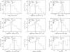 |
Fig. 3 Distributions of a) centimeter luminosity; b) Lyman continuum; c) spectral index; d) electron density; e) emission measure; f) ionized gas mass; g) linear radius of the centimeter source; h) deconvolved angular diameter, θS; and i) peak intensity to flux density ratio, for the centimeter sources detected with ATCA. The numbers at the top of each panel indicate the total number of sources used in the histogram (in some cases we could only use 207 sources, i.e., those with distance determination), and the mean, standard deviation and median values. The vertical dashed line indicates the median value. |
Assuming an uncertainty of 10% on the flux density and angular diameter, one finds that this implies uncertainties of 30% for the emission measure, 20% for the electron density, 20% for the ionized gas mass, and 10% for the Lyman continuum. Note that for extended sources the measured flux density could be a lower limit should the interferometer be filtering extended emission, and the measured size could be underestimated by up to 50% if the source is not Gaussian (see Panagia & Walmsley 1978).
In Col. 12 of Table 5 we give the spectral index (α; Sν ∝ να) estimated from the 18.0 GHz and 22.8 GHz fluxes. However, these values must be taken with caution due to the large uncertainties involved, mainly because the two frequencies are very close and hence the error on α is large. In addition, the 22.8 GHz images could be more affected than the 18.0 GHz images by filtering of extended structures.
In Fig. 3, we show the distribution of the main physical parameters of the centimeter continuum sources. The mean, standard deviation, and median values of each histogram are shown at the top of each panel. In Table 6, we list the median values of these parameters for the whole sample (Col. 3) and for the various classes of objects considered in this paper (Cols. 4−8; see next sections). The median diameters (~0.36 pc), electron densities (~580 cm-3), and emission measures (~7.9 × 104 cm-6 pc) agree with typical values of compact H ii regions (Kurtz 2005), with the observed parameters ranging between those of classical and ultracompact H ii regions.
5.2. Lyman continuum
In Fig. 4 we compare the Lyman continuum, NLy, obtained from the measured radio flux with the bolometric luminosity, Lbol, estimated from the IRAS fluxes (Fontani et al. 2005). We considered a centimeter continuum source to be associated with the IRAS source if their separation is ≤ 60′′ (corresponding to the HPBW of the IRAS satellite at 25 μm). We stress, as explained in Sect. 2, that for those sources for which it was not possible to distinguish between the near and far kinematic distances, the near estimate was arbitrarily assumed.
The red solid curve in Fig. 4 corresponds to the
relationship between NLy and Lbol
expected for an O-B type star. This has been computed by various authors (e.g., Panagia
1973; Thompson 1984; Vacca et al. 1996; Schaerer &
de Koter 1997; Díaz-Miller et al. 1998), resulting in a maximum discrepancy ≲30% among
different calculations. While most points in Fig. 4
fall below the red curve, a significant fraction of the sources happen to lie above it.
This is surprising, as the Lyman continuum from a single star is the maximum value
obtainable for a given bolometric luminosity, as illustrated by the dashed area in the
figure, which corresponds to the expected NLy if
Lbol is due to a stellar cluster. This result has been
obtained by generating a large collection (106) of clusters with sizes ranging
from 5 to 500 000 stars each. The clusters are assembled randomly from a cluster
membership distribution that describes the number of clusters
(Ncl) composed of a given number of stars
(Nst) of the form,  with α = −2. Each cluster
was populated assuming a randomly sampled Chabrier (2005) initial mass function with stellar masses in the range
0.1–120 M⊙. For each cluster we computed the total mass,
bolometric luminosity, maximum stellar mass, and integrated Lyman continuum. The shaded
area in Fig. 4 was produced by plotting at each
bolometric luminosity the range that includes 90% of the simulated clusters.
with α = −2. Each cluster
was populated assuming a randomly sampled Chabrier (2005) initial mass function with stellar masses in the range
0.1–120 M⊙. For each cluster we computed the total mass,
bolometric luminosity, maximum stellar mass, and integrated Lyman continuum. The shaded
area in Fig. 4 was produced by plotting at each
bolometric luminosity the range that includes 90% of the simulated clusters.
How can one explain the presence of so many objects in the forbidden region above the red curve in Fig. 4? A priori several explanations are possible and we discuss them in the following:
-
The radio flux (from which NLy is computed) could be overestimated. In practice, one cannot think of any reason why this should be the case. On the one hand, if the H ii regions were optically thick, density-bound, or dusty, the free-free emission would be reduced and the estimated NLy would be a lower limit. On the other hand, interferometric observations tend to resolve extended emission and rather decrease the measured flux density (and hence the estimated value of NLy). Finally, uncertainties in the flux calibration may reach a few 10%, much less than the observed excess with respect to the single-star curve in Fig. 4 (up to almost 3 orders of magnitude).
-
The bolometric luminosity could be underestimated. Since we derived Lbol from the flux densities reported in the IRAS Point Source Catalog, this explanation is very unlikely. The IRAS HPBW ranges from 0
 5 to 2′ and thus encompasses an area
even larger than that of the observed H ii regions. Consequently, the IRAS
fluxes are more likely overestimating the emission from the relevant sources and the
estimated Lbol is rather an upper limit.
5 to 2′ and thus encompasses an area
even larger than that of the observed H ii regions. Consequently, the IRAS
fluxes are more likely overestimating the emission from the relevant sources and the
estimated Lbol is rather an upper limit. -
The sources in the forbidden region could be Planetary Nebulae (PNe) instead of H ii regions. In this case the value of NLy would be much higher than for a ZAMS star, for the same Lbol. We note that most of the objects above the red curve in Fig. 4 belong to Type 1 and Type 2 (see Sect. 6) and are thus associated with molecular clumps, which appears quite unlikely for an evolved star such as those powering PNe.
-
The source of NLy could be other than a ZAMS star. For example, it has been proposed that UV photons from shocks could be ionizing thermal jets (e.g., Anglada 1996). However, the expected free-free emission at 1.3 cm from such a jet is on the order of 0.1 mJy kpc2, much less than the measured radio luminosities of the objects in the forbidden region – typically 10–106 mJy kpc2. Another possibility is that the UV photons are originating from shocks in the accretion flow onto the protostar/disk system. Although intriguing, this hypothesis is yet to be investigated theoretically and thus must be regarded as purely speculative at present.
Table 6Median values of main physical parameters of the centimeter sources.
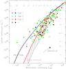
Fig. 4 Lyman continuum, NLy (from Table 5), as a function of the bolometric luminosity, Lbol. Open and filled symbols denote Low and High sources, respectively. The different colors indicate the Type 1 (blue), Type 2 (green), and Type 3 (red), while the black symbols correspond to those centimeter sources not classified in any of the three types (see Sect. 6). The red solid line corresponds to the Lyman continuum of a ZAMS star of a given bolometric luminosity, while the dashed region indicates the expected NLy if Lbol is due to a cluster (see Sect. 5.2 for details). The black solid line corresponds to the Lyman continuum expected from a black-body with the same radius and temperature as a ZAMS star. At the top and right axes we list the spectral type corresponding to a given Lyman continuum and a given bolometric luminosity. The arrow indicates by how much a point should be shifted if its distance is doubled.
-
The distances could be wrong. Indeed, a relatively small error on our distance estimates could significantly affect the position of the corresponding points in Fig. 4. The arrow in this figure indicates by how much a point should be shifted if its distance is doubled. In fact, for many sources we arbitrarily assumed the near kinematic distance, while replacing this with the far distance would certainly move the corresponding points to the right of the red curve. However, even if for all sources above the solid red line the far distance were assumed, still ~50% of them would lie in the forbidden region.
5.3. Source size and electron density relationship
It is interesting to investigate the relationship between density and size in our sample of H ii regions. This is illustrated in Fig. 5, which shows a plot of the electron density, ne, versus the diameter of the H ii region, DH ii, for all our objects. For a given Lyman continuum the relationship between the radius and the electron density of a Strömgren H ii region is fixed. The solid lines drawn in the figure correspond to such a relationship for ZAMS stars of spectral types ranging from B3 to O4. As expected, all points lie in the region spanned by these spectral types.
The result in Fig. 5 is similar to that obtained by
other authors (see e.g. Garay & Lizano 1999;
Martín-Hernández et al. 2003), who noted that the
distribution of the points in the plot appears to be consistent with a steeper
relationship than that expected for a simple Strömgren sphere
( ). However, before drawing this conclusion,
one should take into account any possible observational bias that could affect the
observed distribution of points in that plot. For example, the largest H ii
regions may be resolved out by the interferometric observations, while the smallest could
fall below our sensitivity limit. To take these and other effects into account, we
attempted a more quantitative approach. This consists of comparing the distribution in
Fig. 5 with that obtained assuming that O-B type
stars are distributed in the Galaxy as established by Mottram et al. (2011). The details of our procedure are given in
Appendix A. Here we only stress that with respect
to Mottram et al. we introduced the additional assumption that the number of H ii
regions with electron density ne is given by a function of the
type
). However, before drawing this conclusion,
one should take into account any possible observational bias that could affect the
observed distribution of points in that plot. For example, the largest H ii
regions may be resolved out by the interferometric observations, while the smallest could
fall below our sensitivity limit. To take these and other effects into account, we
attempted a more quantitative approach. This consists of comparing the distribution in
Fig. 5 with that obtained assuming that O-B type
stars are distributed in the Galaxy as established by Mottram et al. (2011). The details of our procedure are given in
Appendix A. Here we only stress that with respect
to Mottram et al. we introduced the additional assumption that the number of H ii
regions with electron density ne is given by a function of the
type  . In practice, our model depends only on
the exponent α and the total number of H ii regions in the
Galaxy, NHII. As shown in Appendix A, we can fit the observed electron density function
. In practice, our model depends only on
the exponent α and the total number of H ii regions in the
Galaxy, NHII. As shown in Appendix A, we can fit the observed electron density function
 and thus obtain the values of the two free
parameters, NHII =
and thus obtain the values of the two free
parameters, NHII =  and α = −0.15 ± 0.1. With
this model one can also estimate the expected distribution of points in the plot of
Fig. 5. This is shown as a color scale, indicating
the number of detectable H ii regions per pixel. Clearly, the expected
distribution is far from homogeneous, and consistent with the distribution of the observed
points. The agreement between model and data can be better appreciated in Figs. A.1 and A.3, where
the best-fit density () and diameter
(
and α = −0.15 ± 0.1. With
this model one can also estimate the expected distribution of points in the plot of
Fig. 5. This is shown as a color scale, indicating
the number of detectable H ii regions per pixel. Clearly, the expected
distribution is far from homogeneous, and consistent with the distribution of the observed
points. The agreement between model and data can be better appreciated in Figs. A.1 and A.3, where
the best-fit density () and diameter
( ) functions are compared to those obtained
from our data.
) functions are compared to those obtained
from our data.
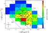 |
Fig. 5 Electron density of the H ii regions detected in our survey versus the corresponding linear diameter. The points denoting the data (listed in Table 5) are overlaid on an image whose intensity (color scale) gives the number of H ii regions expected in each pixel on the basis of the model described in Appendix A. The solid lines correspond to ZAMS stars of spectral types B3, B1, B0, O7, and O4. The cross indicates the 20% error in the electron density and the 10% error in the source size (see Sect. 5.1). |
Although the fit is quite satisfactory, a word of caution is in order. Our findings refer to a sample of objects that is not the result of an unbiased search across the Galactic plane, because our observations were performed toward a limited number of targets selected mostly on the basis of their IRAS colors. However, the adopted selection criteria on the IRAS colors (see Sect. 2) are expected to identify most Galactic H ii regions (and their precursors). It is also worth noting that the number of H ii regions estimated by us (NHII = 15 000) is significantly larger than that obtained by other authors. For instance, Wood & Churchwell (1989) estimated ~1600 embedded O-type stars in the Galaxy, while from the results of Mottram et al. (2011) one may obtain ~8200 Galactic massive young stellar objects and compact H ii regions. However, the former estimate refers only to stars above ~30 000 L⊙ and the latter does not consider extended H ii regions, which can be detected with our observations.
5.4. Background source contamination
Most of the sources in our sample are located in the fourth galactic quadrant, which
covers the range 254° < l < 360°, with a few at
l ≈ 10°. Regarding the galactic latitudes, our sources are confined to
the galactic disk with |b| < 3°, with most of them (85%) restricted to
|b| < 1°. Most of these sources are included in the range of
galactic coordinates covered by recent infrared and submillimeter unbiased surveys (e.g.,
GLIMPSE and MIPSGAL with Spitzer; Hi-GAL with Herschel;
ATLASGAL with APEX) that can be used to construct the spectral energy distributions from
infrared to millimeter wavelengths. This will be the subject of a forthcoming paper
(Sánchez-Monge et al., in prep). The location of our sources within the galactic disk is
consistent with them being associated with star-forming regions, with the centimeter
continuum emission coming from H ii regions (as shown in the previous section).
However, we cannot exclude the possibility that some of the radio continuum sources are in
fact extragalactic sources. Following the appendix of Anglada et al. (1998) and considering our ATCA observations at a
frequency of 20.4 GHz, we can estimate the number of expected background sources as
![Mathematical equation: \begin{equation*} \langle N\rangle =0.041 \left[1-\exp^{-0.109~\theta_\mathrm{FOV}^2}\right] \left(\frac{S_\mathrm{0}}{\mathrm{mJy}}\right)^{-0.75}, \end{equation*}](/articles/aa/full_html/2013/02/aa19890-12/aa19890-12-eq609.png) with θFOV the
field of view in arcmin and S0 the detectable flux density
threshold at the center of the field that we will consider to be 5σ
(~2 mJy). For a field of view of 25, and considering that we have 192
distinct fields, we expect to detect ⟨ N ⟩ ≃ 3 background sources.
Since we have detected a total of 214 centimeter continuum sources, only ~2% of them
could in fact be extragalactic sources.
with θFOV the
field of view in arcmin and S0 the detectable flux density
threshold at the center of the field that we will consider to be 5σ
(~2 mJy). For a field of view of 25, and considering that we have 192
distinct fields, we expect to detect ⟨ N ⟩ ≃ 3 background sources.
Since we have detected a total of 214 centimeter continuum sources, only ~2% of them
could in fact be extragalactic sources.
There are eight sources with high negative spectral indices (<−5) that could be extragalactic non-thermal sources: 10184−5748 0, 10317−5936 0, 13106−6050 0, 13592−6153 0, 14214−6017 0, 15015−5720 0, 16363−4645 0, and 17242−3513 (see Table 5). However, visual inspection of the radio continuum maps reveals that these sources are associated with strong millimeter condensations or infrared sources, and some of them are coincident with or close to H2O masers, suggesting a galactic origin. Also, the spectral indices are too negative even for synchrotron emission from jets found in star-forming regions (e.g., Reid et al. 1995; Carrasco-González et al. 2010). Therefore, these spectral indices are probably the result of filtering out more emission at 22.8 GHz than at 18.0 GHz. Thus, these regions are probably extended and more evolved H ii regions rather than extragalactic sources. Indeed, it is interesting to note that the eight sources with high negative spectral indices correspond to sources located in regions with multiple centimeter sources, suggesting that confusion in combination with the poor uv-coverage of our snapshot observations could complicate the estimate of the flux, eventually resulting in unreliable spectral indices.
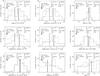 |
Fig. 6 Distributions of a) centimeter luminosity; b) Lyman continuum; c) spectral index; d) electron density; e) emission measure; f) ionized gas mass; g) linear radius of the centimeter source; h) deconvolved angular diameter, θS; and i) peak intensity to flux density ratio, for the centimeter sources associated with Low (dashed line) and High (solid line) regions. The numbers at the top of each panel are as in Fig. 3. The vertical thick lines indicate the median values. |
5.5. Low versus High: centimeter continuum properties
The two groups (High and Low) defined by Palla et al. (1991) to classify the IRAS sources associated with massive star-forming regions have been proposed to include sources in different evolutionary stages, with the High sources being more evolved and more likely associated with UC H ii regions. Several works have studied the molecular and dust content in these two groups of sources. Brand et al. (2001) compared the molecular properties of two samples containing Low and High sources, and reported that molecular clumps associated with Low sources have larger sizes, are less massive, cooler, and less turbulent than High sources. More recently, Fontani et al. (2005) observed different transitions of CS and C17O that trace the dense gas associated with a larger (130) sample of Low sources. These authors found that the temperatures and linewidths estimated for the Low sources were similar to those found toward different samples of High sources (Bronfman et al. 1989; Sridharan et al. 2002; Beuther et al. 2002) with only slightly narrower lines for the Low sources, suggesting that the gas could be more perturbed in High sources because of H ii regions. Beltrán et al. (2006) studied the dust properties by observing the 1.2 mm continuum emission toward a large (235) sample of Low and High sources. The sizes of the clumps, masses, surface densities, and H2 volume densities were similar between the two groups of sources, with only small variations found in the size and mass (slightly larger for High sources). Thus, it seems that there are no clear differences in the molecular and dust properties between High and Low sources.
In this section, we compare the properties of the centimeter emission (that likely traces H ii regions) associated with the two different groups of sources. In our sample – 79 IRAS High sources and 81 IRAS Low sources – the detection rate of centimeter continuum emission is 94% and 93% for High and Low sources, respectively. Thus, there are no differences between both groups regarding the presence of H ii regions. Is there any difference in the physical properties of the H ii regions associated with the High and Low sources? In Fig. 6, we show the distribution of the main physical parameters of the centimeter continuum sources for both groups. The physical properties of the H ii regions in both groups seem to be similar, with values of the electron density, emission measure, flux density, and Lyman continuum slightly higher for High sources (see also the median values listed in the Cols. 4 and 5 of Table 6). Moreover, the plot of the Lyman continuum as a function of the bolometric luminosity (see Fig. 4) does not show large differences between the distribution of High (solid symbols) and that of Low (open symbols) sources. It is worth noting that our detection rates (>90%) seem to contradict those obtained by Molinari et al. (1998a): 43% and 24% for High and Low sources, respectively. However, the higher angular resolution observations of Molinari et al. (~10 times better) could be filtering out the extended H ii regions (still observable in our ATCA observations), which results in a decrease of their detection rates. It is worth noting that Molinari et al. (1996) suggested that Low sources could be contaminated by evolved (and more extended) H ii regions. For the water maser association, Palla et al. (1991) found that the detection rate for High sources (26%) is almost three times higher than that of Low sources (9%). In our sample, we obtain a water maser detection rate of 46% and 33% for the High and Low sources, respectively. A direct comparison of the detection rates between the two works is difficult since the observing conditions (sensitivity and spectral resolution) differ considerably between our observations and those of Palla et al. (1991).
In summary, it seems that the presence of H ii regions or water masers, as well as the properties of the millimeter and dense gas emission, are similar for both groups, suggesting that there may exist more effective criteria to make an evolutionary classification than the infrared colors of Low and High sources. This is discussed in the next section.
6. Evolutionary sequence
6.1. Millimeter and infrared counterparts
In this section, we discuss the association between millimeter and infrared sources with the aim of establishing a classification of the objects based on their emission in the two wavelength regimes. For the millimeter sources, we used the sample of 210 regions, which contain 667 millimeter clumps, studied by Beltrán et al. (2006) with the SEST telescope at 1.2 mm. For the infrared sources we used the MSX Point Source Catalog (Price et al. 1999), which provides information between 8 μm and 21 μm (mid-IR) with an angular resolution (20′′) similar to that of the SEST (24′′) and ATCA (20–25′′) maps. We considered only the MSX sources detected at 21 μm that satisfied one of two additional criteria: (a) quality factor ≥ 3 in the E-band (21.3 μm), i.e., well-detected sources; (b) quality factor 1 or 2 in the E-band, and quality factor ≥ 3 in at least one of the other bands (A: 8.3 μm, C: 12.1 μm, D: 14.7 μm). We used the MSX data instead of other more sensitive and recent surveys (e.g., MIPSGAL at 24 μm) for four reasons: the existence of a point source catalog for the MSX data, which is not yet available for other surveys; the saturation of many regions in our sample in the MIPSGAL images; the similar resolution with our millimeter and centimeter images; and consistency with the method used by Molinari et al. (2008; see next sections).
To determine the association between millimeter and infrared sources, we performed the following analysis. We calculated the angular separation between millimeter and infrared sources and searched for the closest companion of each millimeter source. In the top panel of Fig. 7, we plot the 21 μm-to-1.2 mm flux ratio (hereafter S21 μm / S1.2 mm) versus the angular separation for each pair of millimeter and infrared sources (hereafter Δn). Note that we use a normalized angular separation (to exclude the dependence on distance), computed by dividing the angular separation by the sum of the angular radii of the millimeter and infrared sources. The angular radius is equal to half the angular diameter reported in Beltrán et al. (2006) for the millimeter sources and is assumed to be half the 20′′ HPBW for the MSX sources. We expect is that S21 μm / S1.2 mm could take any value if the millimeter and infrared fluxes come from two different (unrelated) objects, whereas it should span a narrow range of values if the two fluxes belong to the same object (because YSOs have roughly similar spectral energy distributions). We expect that the probability that the MSX source is the real counterpart of the mm source decreases with this separation. This expectation is confirmed by the fact that the flux ratio spans a wider range of values for increasing separation, thus confirming that the MSX source is really associated with the mm source only for sufficiently small Δn. This can be seen in the bottom panel of Fig. 7 (black dots), where the dispersion σr of S21 μm / S1.2 mm appears to decrease below Δn ≃ 0.7, marked by the vertical line in the figure. This normalized separation corresponds approximately to an angular separation between the millimeter and infrared sources of ~15′′ (taking into account the typical sizes of the millimeter sources: ~20−40′′; Beltrán et al. 2006). For a range of distances between 1 and 7 kpc, the resulting spatial separation is ~0.07−0.5 pc.
In addition, we used the Kolmogorov-Smirnov statistical test to compare the S21 μm / S1.2 mm distribution in different bins with the global distribution containing data with Δn > 1. The result is shown by the gray histogram in the bottom panel of Fig. 7, and demonstrates that the distributions for almost all bins with Δn ≲ 1 are statistically different with respect to the global distribution: the test shows that the probability of the distribution in each bin being the same of the global distribution becomes very low (P ≲ 0.3) for Δn ≲ 1. Furthermore, the comparison of the distributions with Δn < 1 and Δn > 1 results in a minimum probability of P ≃ 0.05. The results of the Kolmogorov-Smirnov statistical tests, together with the decrease in the dispersion for Δn ≲ 0.7, are strong evidence of a different behavior between IR-mm associations with respect to the normalized angular separation. We thus conclude that only an IR counterpart satisfying the condition Δn < 0.7 (as a conservative value from the range 0.7–1, corresponding to a spatial separation of 0.07−0.5 pc; see above) is physically associated with the corresponding mm source.
6.2. Source classification
The analysis presented in the previous section allows us to identify three types of YSOs: millimeter sources associated with infrared counterparts, millimeter sources not associated with an infrared source, and infrared sources lying relatively close to millimeter sources (and therefore likely associated with star forming regions) but not associated with them. While the millimeter continuum emission probably comes from dust envelopes around YSOs, we cannot be sure that the same is true for the infrared emission, which could be produced by more evolved objects or background/foreground stars. With the aim of selecting only YSO candidates, we applied the following restriction to our catalog of infrared-only sources: F21 μm ≥ F15 μm and F21 μm ≥ F12 μm in the MSX bands, to ensure an increasing spectral energy distribution at infrared wavelengths typical of YSOs5. In Fig. 8 we plot the ratio S21 μm / S1.2 mm versus the normalized angular separation, taking into account the previous restriction, and considering the sources within the ATCA fields. For millimeter sources without an infrared counterpart we assumed a flux at 21 μm equal to an upper limit four times the rms noise level of the MSX map, and, similarly, for sources only detected at infrared wavelengths we assumed the flux at 1.2 mm to be an upper limit equal to four times the rms noise level of the millimeter map. The resulting plot shows the three different groups of sources: Type 1, only millimeter continuum sources (blue circles), Type 2, millimeter continuum sources associated with an infrared counterpart (green dots), and Type 3, infrared sources located far from a millimeter source (red stars).
These three groups of sources correspond to the classification proposed by Molinari et al. (2008) from a study of the infrared and millimeter properties of a sample of 42 regions. Molinari et al. (2008) checked by eye the infrared and millimeter emission, and by fitting different spectral energy distributions, identified associations between infrared and millimeter sources. A simple model allowed the authors to establish an evolutionary sequence, in order of increasing age going from Type 1 to Type 3 objects. In the sample studied by Molinari et al. (2008) there are 33 millimeter sources taken from Beltrán et al. (2006) that are included in our analysis. Taking into account our method for determining associations between infrared and millimeter sources, and comparing it with the results of Molinari et al. (2008), we conclude that ~80% of the 33 sources agree with respect to the source classification in Type 1, Type 2, or Type 3. Thus, our more automatic classification method, used for the classification in different evolutionary stages of our sources, agrees with the Molinari et al. method, and will be used for further analysis. In Tables 7–9, we list the millimeter and/or infrared sources classified in the three evolutionary stages.
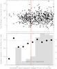 |
Fig. 7 Top: 21 μm-to-1.2 mm flux ratio versus the normalized angular separation between millimeter and infrared sources (see Sect. 6.1 for details). The flux at 21 μm flux is obtained from the MSX catalog and the flux at 1.2 mm is obtained from Beltrán et al. (2006). Bottom: standard deviation in the 21 μm-to-1.2 mm flux ratio versus the normalized angular separation (black dots). The dashed horizontal blue line corresponds to the standard deviation (≃0.57) for data with Δn > 0.7. The gray histogram indicates the probability that the distribution of data within one bin is the same as the global distribution with Δn > 1, using the Kolmogorov-Smirnov statistical test. The red vertical line indicates the normalized angular separation that distinguishes between millimeter and infrared associated and non-associated sources (see Sect. 6.1). |
At this point, we can compare the evolutionary classification derived from the IR–mm analysis with the High–Low classification obtained from the IRAS colors. If we consider the millimeter (SEST) and infrared (MSX) sources located within an IRAS beam (~2′), we find that an IRAS source with Low colors contains 42%, 27%, and 31% of Type 1, Type 2, and Type 3 sources, respectively; while within the beam of a High IRAS source we can find 23%, 37%, and 40% of Type 1, Type 2, and Type 3 sources, respectively. This result agrees with the analysis by Molinari et al. (2008) on a much smaller sample and suggests that less evolved sources (Type 1) are typically found closer to a Low IRAS source than more evolved sources (Type 2 and Type 3). However, evolved objects can also be found associated with Low IRAS sources, as shown by distinct studies (e.g., Molinari et al. 1998a, 2000), and as expected by the high detection rate of H ii regions found associated with Low sources (see Sect. 5.5).
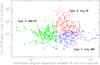 |
Fig. 8 21 μm to 1.2 mm flux ratio versus the normalized angular separation between millimeter and infrared sources. Blue open circles correspond to Type 1 sources (only millimeter emission), green filled circles correspond to Type 2 sources (association between millimeter and infrared emission), and red stars correspond to Type 3 sources (only infrared emission). Blue symbols (millimeter-only sources) are upper limits in which we have considered an upper limit of four times the rms noise in the MSX image. Red symbols (infrared-only sources) are lower limits in which we considered an upper limit of four times the rms noise in the SEST image. |
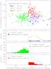 |
Fig. 9 Associations with H ii regions. Top: 21 μm to 1.2 mm flux ratio versus the normalized angular separation between millimeter and infrared sources as in Fig. 8. Blue symbols correspond to Type 1 sources (only millimeter emission), green symbols correspond to Type 2 sources (association between millimeter and infrared emission); and red symbols correspond to Type 3 sources (only infrared emission). Colored filled dots show those objects associated with H ii regions detected with ATCA (see Table 3). The numbers at the top of the panel indicate the percentage of association of H ii regions in each of three groups. Bottom: histograms of the normalized angular separation for the different groups. The solid black lines correspond to all sources of each group and the colored filled histograms correspond those objects associated with H ii regions. |
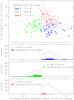 |
Fig. 10 Associations with H2O masers. Top: 21 μm to 1.2 mm flux ratio versus the normalized angular separation between millimeter and infrared sources as in Fig. 9. Colored filled dots show those objects associated with H2O masers detected with ATCA (see Table 4). The numbers at the top of the panel indicate the percentage of association of H2O masers in each of three groups. Bottom: histograms of the normalized angular separation for the different groups. The solid black lines correspond to all sources of each group and the colored filled histograms correspond those objects associated with H2O masers. |
6.3. HII regions and H2O masers
In this section, we investigate the presence of H ii regions and water masers in the three evolutionary stages (see Figs. 9 and 10). We used the same criteria to establish if an H ii region or a water maser is associated with a millimeter or infrared source, i.e., the normalized distance must be <0.7, using the size listed in Table 3 for the H ii regions, and the HPBW at 22 GHz for the water maser (the water maser emission is unresolved in our observations). In Fig. 11, we show a simple sketch that indicates the associations with H ii regions and water masers for the three source types, and in Table 10, we summarize the number of sources and percentages of associations with H ii regions and water masers in the Type 1, Type 2, and Type 3 sources.
Regarding the H ii regions, most of the centimeter continuum sources appear associated with Type 2 and Type 3 objects (corresponding to 72% of all detected sources), and only a low percentage (7%) are associated with Type 1 objects. The remaining 21% correspond to H ii regions not associated with millimeter or infrared sources. These results indicate on the one hand that for the first evolutionary stage (Type 1) the H ii region has not developed yet (only 8% of Type 1 sources are associated with H ii regions; see Fig. 9), and that the massive protostar begins to ionize the surrounding gas when the millimeter core is detectable at infrared wavelengths (75% of Type 2 sources are associated with H ii regions). On the other hand, in the last stages when the infrared source dominates the emission and most of the dusty clump has been destroyed (i.e., Type 3), one would expect that the association of H ii regions with infrared sources would be higher than for Type 2 objects. In contrast, we observe a decrease in the percentage of associations (from 75% to 28%). We investigated if there was a contamination of infrared sources not associated with star formation in our sample of Type 3 objects. From MSX color–color diagrams we do not detect a differentiation between infrared sources associated with H ii regions and not associated infrared sources. In Fig. 12, we show two MSX-color histograms for Type 2 and Type 3 objects. We can see that for each type the distribution of sources associated with H ii regions is similar to the total distribution, and therefore we conclude that no significant contamination of not associated sources should affect the Type 3 sample.
In Fig. 13, we show the distribution of the physical parameters of the H ii regions associated with the three types of objects. It seems that the continuum flux and Lyman continuum is greater in more evolved objects (Type 2 and Type 3) than in the regions associated with only millimeter emission (see last three columns of Table 6). Focusing on the two more evolved types, we can see that the electron density and the emission measure decrease from Type 2 to Type 3, while the size increases, as expected if the H ii regions associated with Type 3 objects are more evolved. Taking this into account, the relatively low percentage of association for Type 3 objects could be understood in terms of the properties of their H ii regions: if the H ii region is larger and has a lower density, our snapshot observations would be inadequate to detect these H ii regions, and accordingly the percentage of associations would appear reduced in comparison with Type 2 objects, the latter being associated with more compact and dense H ii regions, which are more easily detectable in our interferometric observations. The small number of H ii regions associated with Type 1 objects makes it difficult to derive typical values for these H ii regions. However, it is worth noting that the sizes of these centimeter continuum sources are larger than those of Type 2 and Type 3 objects, contrary to what is expected if the H ii regions of Type 1 objects are less evolved. Similarly, low values of the density and emission measure, due to the large sizes, are also unexpected for less evolved H ii regions. An inspection of the maps for these sources reveals that most of these centimeter continuum sources are faint, which results in a poor estimation of the size, and in other cases a faint MSX infrared emission appears at the position of the H ii region, suggesting that there could be some contamination of Type 2 objects. This would imply that the detection rate of H ii regions in the Type 1 group would be lower, as expected if these sources are younger.
In Fig. 14, we report the distribution of normalized distances between the millimeter source and the nearest centimeter continuum source. The distribution for Type 2 objects peaks at smaller normalized distances than for millimeter-only Type 1 objects. In massive YSOs the association with centimeter continuum emission typically indicates the developing of an H ii region and consequently, objects that have reached the ZAMS. The results shown in Fig. 14 agree with the tentative result shown by Molinari et al. (2008) in a smaller sample.
 |
Fig. 11 Sketch showing the number of sources in each of the three types of sources. We indicate the number of sources associated with only H ii regions, only water maser emission, and both H ii regions and water masers. |
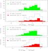 |
Fig. 12 Distributions of the MSX colors [21 μm–8 μm] (two top panels) and [21 μm–12 μm] (two bottom panels) for Type 2 (green histograms) and Type 3 (red histograms) sources. The solid black lines show the total number of sources of each group, and the colored filled histograms show the sources associated with H ii regions. |
Regarding the water maser emission (see Fig. 10), we find that most of the water masers are associated with the earliest stages (67% for Type 1 and 2), and only few of them (7%) are associated with Type 3 objects. The evolution might begin with millimeter-only objects (Type 1) with only some of them associated with water maser emission. As the object evolves and becomes visible in the infrared (Type 2), the number of masers associated with these objects increases by a factor of 2, most of them being associated with H ii regions. Finally, as the object evolves and becomes less embedded, the association with masers also decreases.
The sketch shown in Fig. 11 summarizes the results found in this work: while the H ii region phase is dominant in the Type 2 and Type 3 objectsepsfig, the water masers are most likely associated with the first stages. These results confirm the evolutionary classification proposed by Molinari et al. (2008), in which Type 1 sources would be high-mass protostars embedded in dust clumps with maser emission but still not developing an H ii region, Type 2 sources would correspond to ZAMS OB stars with developed H ii regions, but still embedded in dust condensations and associated with maser emission, and Type 3 sources would be more evolved ZAMS OB stars surrounded only by remnants of their parental clouds and with more extended and less dense H ii regions. This scenario is consistent with the evolutionary schemes presented by Ellingsen et al. (2007) and Breen et al. (2010), in which water masers appear first in the evolution of a massive protostar, coexist with the H ii regions, and disappear while the H ii regions are still detectable. Similarly, the evolutionary stages proposed by Molinari et al. (2008) and this work compare well with the evolutionary classifications described by Beuther et al. (2007) or Zinnecker & Yorke (2007): Type 1 sources would correspond to high-mass starless cores (HMSCs) or young high-mass protostellar objects (HMPOs) that are likely associated with infrared dark clouds (IRDCs) and hot molecular cores (HMCs), Type 2 sources would be mainly evolved HMPOs or final stars associated with ultracompact H ii regions, and Type 3 objects would be final stars associated with compact or classical H ii regions.
Number (and percentage) of sources associated with H ii regions and water masers for Type 1, Type 2, and Type 3.
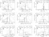 |
Fig. 13 Distributions of a) centimeter luminosity; b) Lyman continuum; c) spectral index; d) electron density; e) emission measure; f) ionized gas mass; g) linear radius of the centimeter source; h) deconvolved angular diameter, θS; and i) peak intensity to flux density ratio, for the centimeter sources in the evolutionary stages Type 1 (gray filled), Type 2 (dashed line), and Type 3 (solid line). The numbers at the top of each panel are as in Fig. 3. The vertical thick lines indicate the median values. |
7. Summary
We have carried out ATCA observations of the H2O maser line and radio continuum emission at 18.0 GHz and 22.8 GHz toward a sample of 192 southern (δ < −30°) massive star-forming regions that contain several clumps already imaged at 1.2 mm (Beltrán et al. 2006). The sample consisted of 160 fields centered on an IRAS source plus 32 fields centered on a millimeter clump located >150′′ from an IRAS source. In total we observed 79 High IRAS sources and 81 Low IRAS sources (according to the criteria of Palla et al. 1991). The main findings obtained in this work are these:
-
We detected centimeter continuum emission in 169 out of 192 fields, corresponding to a detection rate of 88%. In total, 12% of the fields do not show centimeter continuum emission (up to a level of ~2 mJy), in 68% we found a single component (with an angular resolution of ~20′′), and in 20% we found multiple components.
-
For the water maser emission, we detected 85 distinct components in 78 fields, corresponding to a detection rate of 41%. Owing to the poor spectral resolution (12.5 km s-1), we are probably detecting only relatively strong (≳1 Jy) water masers.
-
Assuming that the centimeter continuum emission comes from optically thin H ii regions, we derived the physical parameters obtaining values in agreement with compact H ii regions (diameters ~0.36 pc, electron densities ~580 cm-3, emission measures ~7.9 × 105 cm-6 pc). The derived number of Lyman continuum photons spans a range between 1044 s-1 and 1050 s-1, corresponding to spectral types B5 to O5.
-
No large differences are found when studying the association or physical parameters of the H ii regions in the High and Low groups of sources. We found an H ii region detection rate of 94% and 93% for High and Low sources, respectively, with the electron density and emission measure slightly higher for High sources. For the water maser emission, we found a detection rate of 46% and 33% for High and Low sources. These detection rates differ from previous results (e.g., Palla et al. 1991; Molinari et al. 1998a) probably because of the different observing conditions (sensitivity, angular resolution, and spectral resolution).
-
We compared the Lyman continuum obtained from the measured radio flux with the bolometric luminosity estimated from the IRAS fluxes. Several sources (preferentially associated with the earliest evolutionary stages and with B-type stars) show an excess of Lyman continuum that cannot be easily explained. If the distances, which are the main source of uncertainty in this comparison, are confirmed (or more accurately estimated) and the excess of Lyman continuum is still considerable, we should consider that B-stars could emit in the UV range much stronger than predicted by standard models of stellar atmospheres or that there exists another source of Lyman continuum in addition to the ZAMS star.
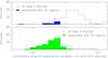
Fig. 14 Histograms of the normalized angular separation between the millimeter continuum source and the nearest H ii region for Type 1 (top panel) and Type 2 (bottom panel) sources.
-
We investigated the relation of the electron density and size of the H ii regions and compared our distribution with that obtained assuming that O-B type stars are distributed in the Galaxy as proposed by Mottram et al. (2011). From this analysis, we estimate the number of compact and extended H ii regions in the Galaxy to be ~15 000.
-
H ii regions are mainly associated (72%) with Type 2 and Type 3 sources, while only 7% are associated with Type 1 objects. Water masers are mainly associated with Type 1 and Type 2 objects: 67% compared to the 7% association with Type 3 sources.
-
H ii regions associated with Type 3 sources are larger in size and less dense than those associated with Type 2 sources, as expected if the H ii region expands as it evolves.
-
The detailed analysis of each group results in an evolutionary trend for the association of H ii regions (8% for Type 1, 75% for Type 2, and 28% for Type 3) and water masers (13% for Type 1, 26% for Type 2, and 3% for Type 3). This scenario is consistent with the evolutionary schemes presented by Ellingsen et al. (2007) and Breen et al. (2010), in which water masers appear first in the evolution of a massive protostar, coexist with the H ii regions, and disappear while the H ii regions are still detectable. Our results of H ii regions and H2O maser associations with different evolutionary types confirm the evolutionary classification proposed by Molinari et al. (2008), which compares well with the evolutionary classifications described by Beuther et al. (2007) and Zinnecker & Yorke (2007). Thus, Type 1 sources, which are associated with the earliest stages in our evolutionary scheme, appear to be good candidates to distinguish between the different theoretical models of massive star formation.
Online material
Appendix A: Model description
The purpose of this appendix is to give an estimate of the number of H ii regions that can be detected in our survey. This obviously depends on the physical parameters of the H ii regions, their distances, and the sensitivity of our observations. We assumed that:
-
the H ii regions are spatially distributed across the Galaxy according to the equation
![Mathematical equation: \appendix \setcounter{section}{1} \begin{eqnarray*} \fvol & = & \frac{\exp\left[-\frac{|z|}{\zd}\right]}{2\zd} \, \frac{\exp\left[-\left(\frac{R-\Ro}{\Rd}\right)^2\right] - \exp\left[-\left(\frac{R-\Ro}{\Rh}\right)^2\right]} {\pi\left[\Rd\left(\Rd+\sqrt{\pi}\Ro\right) - \Rh\left(\Rh+\sqrt{\pi}\Ro\right)\right]} \nonumber \\ & & \Leftrightarrow\ R\ge\Ro \\ \fvol & = & 0 ~~\Leftrightarrow\ ~~R<\Ro, \end{eqnarray*}](/articles/aa/full_html/2013/02/aa19890-12/aa19890-12-eq639.png) which is the same as Eq. (1) of
Mottram et al. (2011), normalized in such a
way that
which is the same as Eq. (1) of
Mottram et al. (2011), normalized in such a
way that  ; here R is the
galactocentric distance, z the height on the Galactic plane,
Ro = 2.2 kpc,
Rd = 6.99 kpc,
Rh = 1.71 kpc, and
zd = 0.039 kpc (from Mottram et al. 2011);
; here R is the
galactocentric distance, z the height on the Galactic plane,
Ro = 2.2 kpc,
Rd = 6.99 kpc,
Rh = 1.71 kpc, and
zd = 0.039 kpc (from Mottram et al. 2011); -
the H ii regions are homogeneous Strömgren spheres ionized by stars with luminosities in the range 103–106 L⊙;
-
the normalized luminosity function (
 ) of the ionizing star(s) is
described by the power law
) of the ionizing star(s) is
described by the power law  with
L1 = 103 L⊙,
L2 = 106 L⊙,
and β = −0.9, as found by Mottram et al. (2011);
with
L1 = 103 L⊙,
L2 = 106 L⊙,
and β = −0.9, as found by Mottram et al. (2011); -
the normalized electron density distribution (
 ) is also described by a power law,
i.e.,
) is also described by a power law,
i.e.,  with
ne1 = 30 cm-3 and
ne2 = 2 × 104 cm-3
to span the range of ne in Fig. 5.
with
ne1 = 30 cm-3 and
ne2 = 2 × 104 cm-3
to span the range of ne in Fig. 5.
Under these assumptions, the number of Galactic H ii regions per unit volume,
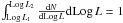
dex in luminosity, and dex in electron density is given by the expression  (A.1)where NHII is
the total number of H ii regions. There are only two free parameters in this
model: the index α and NHII. To find the
corresponding values, we can fit the electron density function obtained from our data
that is represented by the points with error bars in Fig. A.1. The number of H ii regions in each
ne bin of this figure can be calculated from the model in
the following way. The volume of the Galaxy is divided into a suitable number of cells
in cylindrical coordinates. For each of these, Eq. (A.1) is used to calculate the number of H ii regions
contained in that cell, spanning all luminosities in the range
L1–L2, and with density
falling in the chosen bin. In this process, only cells falling in the region surveyed by
us (i.e., those with 254 < l < 360° and
|b| < 10°) were counted. Moreover, for each L the
corresponding Lyman continuum, NLy, was computed assuming
the relationship for a cluster rather than that for a single star (see Sect. 5.1), as it seems unlikely that H ii regions
with linear diameters up to 3 pc may be ionized by only one star. From
ne and NLy one can calculate
the diameter of the Strömgren H ii region,
DH ii, and the corresponding angular diameter
and radio flux measured in the instrumental beam.
(A.1)where NHII is
the total number of H ii regions. There are only two free parameters in this
model: the index α and NHII. To find the
corresponding values, we can fit the electron density function obtained from our data
that is represented by the points with error bars in Fig. A.1. The number of H ii regions in each
ne bin of this figure can be calculated from the model in
the following way. The volume of the Galaxy is divided into a suitable number of cells
in cylindrical coordinates. For each of these, Eq. (A.1) is used to calculate the number of H ii regions
contained in that cell, spanning all luminosities in the range
L1–L2, and with density
falling in the chosen bin. In this process, only cells falling in the region surveyed by
us (i.e., those with 254 < l < 360° and
|b| < 10°) were counted. Moreover, for each L the
corresponding Lyman continuum, NLy, was computed assuming
the relationship for a cluster rather than that for a single star (see Sect. 5.1), as it seems unlikely that H ii regions
with linear diameters up to 3 pc may be ionized by only one star. From
ne and NLy one can calculate
the diameter of the Strömgren H ii region,
DH ii, and the corresponding angular diameter
and radio flux measured in the instrumental beam.
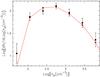 |
Fig. A.1 Electron density function obtained from the data (points with error bars) and best fit from the model (solid line) for α = −0.15 and NHII = 15 000. |
To take into account the bias due to the source selection criteria as well as those introduced by the limited sensitivity of the observations, we took into account only the sources that satisfy the following requirements:
-
L / (4πd2) > 1.6 L⊙ kpc-2, the minimum bolometric flux of the IRAS sources selected by Palla et al. (1991) and Fontani et al. (2005);
-
radio flux above 0.9 mJy beam-1, the mean 3σ sensitivity of our maps;
-
angular diameter below 60′′, the maximum size imaged in our interferometric observations.
The best fit to the electron density function is compared to the data in Fig. A.1. This fit was obtained with
χ2 minimization by varying the two free parameters of the
models over a sufficiently wide range of values. This is illustrated in Fig. A.2, where the χ2 is
plotted as a function of α and NHII. The
thick contour corresponds to the minimum χ2 value (4.64)
plus 2.3, which gives the 1σ confidence level according to Table 1 of
Lampton et al. (1976). We conclude that the best
fit is obtained for NHII =
15 000 and α = −0.15 ± 0.1 As
previously explained, for given ne and
NLy, the H ii region size is univocally
determined. This means that knowledge of the density function
provides us also with the analogous
function for the linear diameter, . The latter is shown in Fig. A.3 and compared to the observed distribution.
Clearly, the two are quite consistent for all diameters, with some discrepancy for the
largest DH ii, where the model appears to
overestimate the measured value. However, the largest H ii regions are also the
most difficult to image with an interferometer, and this may explain this small
discrepancy.
and α = −0.15 ± 0.1 As
previously explained, for given ne and
NLy, the H ii region size is univocally
determined. This means that knowledge of the density function
provides us also with the analogous
function for the linear diameter, . The latter is shown in Fig. A.3 and compared to the observed distribution.
Clearly, the two are quite consistent for all diameters, with some discrepancy for the
largest DH ii, where the model appears to
overestimate the measured value. However, the largest H ii regions are also the
most difficult to image with an interferometer, and this may explain this small
discrepancy.
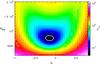 |
Fig. A.2 χ2 obtained by comparing the ne function from the model to that obtained from the data (see Fig. A.1) as a function of the two free parameters, α and NHII. The minimum value (4.64) is obtained for α = −0.15 and NHII = 15 000. The thick contour corresponds to χ2 exceeding the minimum value by 2.3, as recommended by Lampton et al. (1976) to estimate the 1σ confidence level. |
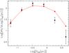 |
Fig. A.3 H ii region diameter function obtained from the data (points with error bars) and from the same model fit (solid line) as in Fig. A.1. |
Appendix B: Figures
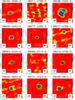 |
Fig. B.1 ATCA continuum images at 18.0 GHz (color scale, units mJy beam-1) and 22.8 GHz (contours). Synthesized beams are indicated at the bottom left (18.0 GHz) and right (22.8 GHz) corners (see Table 1 for values). The primary beam at 22.8 GHz is indicated with the dashed gray circle. When a distance is available, the spatial scale corresponding to 80′′ is indicated at the top of the panel. White stars show the position of water masers (see Table 4). |
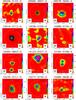 |
Fig. B.1 continued. |
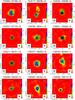 |
Fig. B.1 continued. |
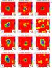 |
Fig. B.1 continued. |
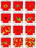 |
Fig. B.1 continued. |
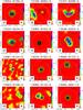 |
Fig. B.1 continued. |
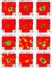 |
Fig. B.1 continued. |
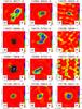 |
Fig. B.1 continued. |
 |
Fig. B.1 continued. |
 |
Fig. B.1 continued. |
 |
Fig. B.1 continued. |
 |
Fig. B.1 continued. |
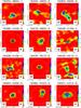 |
Fig. B.1 continued. |
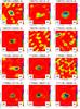 |
Fig. B.1 continued. |
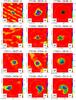 |
Fig. B.1 continued. |
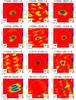 |
Fig. B.1 continued. |
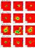 |
Fig. B.2 ATCA, SEST, and MSX maps. For each source we show three panels: left: 21 μm MSX image (color scale) and 1.2 mm SEST image (contours), middle: 1.2 mm SEST image (color scale) and 18.0 GHz ATCA image (contours), and right: 21 μm MSX image (color scale, as in left panel) and 18.0 GHz ATCA image (contours). The spatial scale is shown in sources with distance determination. The primary beam of the ATCA image is shown as a white dashed circle. Water masers are shown as star symbols. |
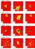 |
Fig. B.2 continued. |
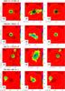 |
Fig. B.2 continued. |
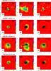 |
Fig. B.2 continued. |
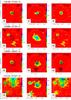 |
Fig. B.2 continued. |
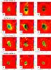 |
Fig. B.2 continued. |
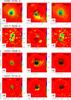 |
Fig. B.2 continued. |
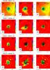 |
Fig. B.2 continued. |
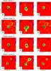 |
Fig. B.2 continued. |
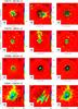 |
Fig. B.2 continued. |
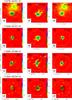 |
Fig. B.2 continued. |
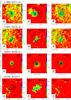 |
Fig. B.2 continued. |
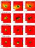 |
Fig. B.2 continued. |
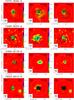 |
Fig. B.2 continued. |
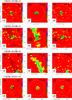 |
Fig. B.2 continued. |
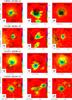 |
Fig. B.2 continued. |
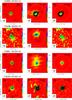 |
Fig. B.2 continued. |
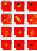 |
Fig. B.2 continued. |
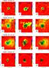 |
Fig. B.2 continued. |
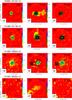 |
Fig. B.2 continued. |
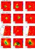 |
Fig. B.2 continued. |
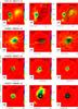 |
Fig. B.2 continued. |
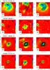 |
Fig. B.2 continued. |
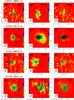 |
Fig. B.2 continued. |
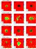 |
Fig. B.2 continued. |
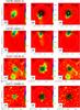 |
Fig. B.2 continued. |
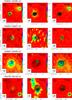 |
Fig. B.2 continued. |
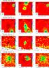 |
Fig. B.2 continued. |
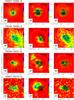 |
Fig. B.2 continued. |
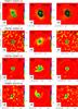 |
Fig. B.2 continued. |
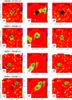 |
Fig. B.2 continued. |
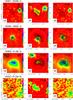 |
Fig. B.2 continued. |
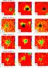 |
Fig. B.2 continued. |
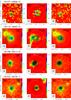 |
Fig. B.2 continued. |
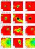 |
Fig. B.2 continued. |
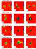 |
Fig. B.2 continued. |
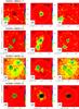 |
Fig. B.2 continued. |
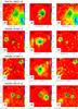 |
Fig. B.2 continued. |
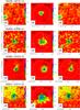 |
Fig. B.2 continued. |
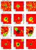 |
Fig. B.2 continued. |
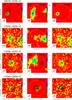 |
Fig. B.2 continued. |
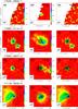 |
Fig. B.2 continued. |
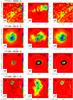 |
Fig. B.2 continued. |
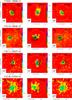 |
Fig. B.2 continued. |
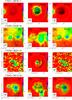 |
Fig. B.2 continued. |
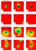 |
Fig. B.2 continued. |
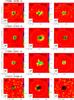 |
Fig. B.2 continued. |
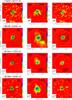 |
Fig. B.2 continued. |
Most of the distance estimates are obtained from spectral line observations pointing toward an IRAS source. We assumed that the millimeter sources detected in the SEST fields surrounding an IRAS source (although not coincident) are located at the same kinematic distance (following the analysis carried out by Beltrán et al. 2006).
In Beltrán et al. (2006) the coordinates of the phase centers reported in their Table 1 for two sources were slightly wrong. The correct coordinates for the SEST observations were α = 16:12:42.7, δ = −51:45:11 for 16085−5138; and α = 17:25:42.0, δ = −36:21:57 for 17221−3619.
The gain calibrators were 0826−373, 1004−50, 1045−62, 1059−63, 1129−58, J1326−5256, 1352−63, 1511−55, 1613−586, 1646−5, 1710−269, 1714−336, 1830−210, and 1923 + 210.
The peak separation in the images at the two frequencies (18.0 GHz and 22.8 GHz) is typically ≲5′′, smaller than the synthesized beam.
Acknowledgments
We thank the anonymous referee for his/her comments. The figures of this paper were made with the software package Greg of GILDAS (http://www.iram.fr/IRAMFR/GILDAS).
References
- Anglada, G. 1996, Radio Emission from the Stars and the Sun, 93, 3 [Google Scholar]
- Anglada, G., Villuendas, E., Estalella, R., et al. 1998, AJ, 116, 2953 [NASA ADS] [CrossRef] [Google Scholar]
- Beltrán, M. T., Brand, J., Cesaroni, R., et al. 2006, A&A, 447, 221 [NASA ADS] [CrossRef] [EDP Sciences] [MathSciNet] [Google Scholar]
- Beuther, H., Schilke, P., Menten, K. M., et al. 2002, ApJ, 566, 945 [NASA ADS] [CrossRef] [Google Scholar]
- Beuther, H., Churchwell, E. B., McKee, C. F., & Tan, J. C. 2007, Protostars and Planets V, 165 [Google Scholar]
- Bonnell, I. A., Vine, S. G., & Bate, M. R. 2004, MNRAS, 349, 735 [NASA ADS] [CrossRef] [Google Scholar]
- Brand, J., Cesaroni, R., Palla, F., & Molinari, S. 2001, A&A, 370, 230 [NASA ADS] [CrossRef] [EDP Sciences] [Google Scholar]
- Breen, S. L., Caswell, J. L., Ellingsen, S. P., & Phillips, C. J. 2010, MNRAS, 406, 1487 [NASA ADS] [Google Scholar]
- Bronfman, L., Alvarez, H., Cohen, R. S., & Thaddeus, P. 1989, ApJS, 71, 481 [NASA ADS] [CrossRef] [Google Scholar]
- Carrasco-González, C., Rodríguez, L. F., Anglada, G., et al. 2010, Science, 330, 1209 [NASA ADS] [CrossRef] [PubMed] [Google Scholar]
- Chabrier, G. 2005, The Initial Mass Function 50 Years Later, 327, 41 [Google Scholar]
- Diaz-Miller, R. I., Franco, J., & Shore, S. N. 1998, ApJ, 501, 192 [NASA ADS] [CrossRef] [Google Scholar]
- Ellingsen, S. P., Voronkov, M. A., Cragg, D. M., et al. 2007, IAU Symp., 242, 213 [NASA ADS] [Google Scholar]
- Faúndez, S., Bronfman, L., Garay, G., et al. 2004, A&A, 426, 97 [NASA ADS] [CrossRef] [EDP Sciences] [Google Scholar]
- Faustini, F., Molinari, S., Testi, L., & Brand, J. 2009, A&A, 503, 801 [NASA ADS] [CrossRef] [EDP Sciences] [Google Scholar]
- Felli, M., Brand, J., Cesaroni, R., et al. 2007, A&A, 476, 373 [NASA ADS] [CrossRef] [EDP Sciences] [Google Scholar]
- Fontani, F., Cesaroni, R., Testi, L., et al. 2004a, A&A, 414, 299 [NASA ADS] [CrossRef] [EDP Sciences] [Google Scholar]
- Fontani, F., Cesaroni, R., Testi, L., et al. 2004b, A&A, 424, 179 [NASA ADS] [CrossRef] [EDP Sciences] [Google Scholar]
- Fontani, F., Beltrán, M. T., Brand, J., et al. 2005, A&A, 432, 921 [NASA ADS] [CrossRef] [EDP Sciences] [Google Scholar]
- Fontani, F., Caselli, P., Crapsi, A., et al. 2006, A&A, 460, 709 [NASA ADS] [CrossRef] [EDP Sciences] [Google Scholar]
- Garay, G., & Lizano, S. 1999, PASP, 111, 1049 [NASA ADS] [CrossRef] [Google Scholar]
- Grave, J. M. C., & Kumar, M. S. N. 2009, A&A, 498, 147 [NASA ADS] [CrossRef] [EDP Sciences] [Google Scholar]
- Green, J. A., & McClure-Griffiths, N. M. 2011, MNRAS, 417, 2500 [NASA ADS] [CrossRef] [Google Scholar]
- Gwinn, C. R. 1994, ApJ, 429, 253 [NASA ADS] [CrossRef] [Google Scholar]
- Hill, T., Burton, M. G., Minier, V., et al. 2005, MNRAS, 363, 405 [NASA ADS] [CrossRef] [Google Scholar]
- Hoare, M. G., Lumsden, S. L., Oudmaijer, R. D., et al. 2004, Milky Way Surveys: The Structure and Evolution of our Galaxy, 317, 156 [Google Scholar]
- Krumholz, M. R., Klein, R. I., McKee, C. F., Offner, S. S. R., & Cunningham, A. J. 2009, Science, 323, 754 [NASA ADS] [CrossRef] [PubMed] [Google Scholar]
- Kuiper, R., Klahr, H., Beuther, H., & Henning, T. 2010, ApJ, 722, 1556 [CrossRef] [Google Scholar]
- Kurtz, S. 2005, in Massive Star Birth: A Crossroads of Astrophysics, eds. R. Cesaroni, M. Felli, E. Churchwell, & M. Walmsley (Cambridge: Cambridge Univ. Press), IAU Symp., 227, 111 [Google Scholar]
- Kurtz, S., Churchwell, E., & Wood, D. O. S. 1994, ApJS, 91, 659 [NASA ADS] [CrossRef] [Google Scholar]
- Lampton, M., Margon, B., & Bowyer, S. 1976, ApJ, 208, 177 [NASA ADS] [CrossRef] [Google Scholar]
- McKee, C. F., & Tan, J. C. 2003, ApJ, 585, 850 [NASA ADS] [CrossRef] [MathSciNet] [Google Scholar]
- Martins, F., Schaerer, D., & Hillier, D. J. 2005, A&A, 436, 1049 [NASA ADS] [CrossRef] [EDP Sciences] [Google Scholar]
- Martín-Hernández, N. L., van der Hulst, J. M., & Tielens, A. G. G. M. 2003, A&A, 407, 957 [NASA ADS] [CrossRef] [EDP Sciences] [Google Scholar]
- Mezger, P. G., & Henderson, A. P. 1967, ApJ, 147, 471 [NASA ADS] [CrossRef] [Google Scholar]
- Moscadelli, L., Cesaroni, R., Rioja, M. J., Dodson, R., & Reid, M. J. 2011, A&A, 526, A66 [NASA ADS] [CrossRef] [EDP Sciences] [Google Scholar]
- Molinari, S., Brand, J., Cesaroni, R., & Palla, F. 1996, A&A, 308, 573 [NASA ADS] [Google Scholar]
- Molinari, S., Brand, J., Cesaroni, R., Palla, F., & Palumbo, G. G. C. 1998a, A&A, 336, 339 [NASA ADS] [Google Scholar]
- Molinari, S., Testi, L., Brand, J., Cesaroni, R., & Palla, F. 1998b, ApJ, 505, L39 [NASA ADS] [CrossRef] [Google Scholar]
- Molinari, S., Brand, J., Cesaroni, R., & Palla, F. 2000, A&A, 355, 617 [NASA ADS] [Google Scholar]
- Molinari, S., Testi, L., Rodríguez, L. F., & Zhang, Q. 2002, ApJ, 570, 758 [NASA ADS] [CrossRef] [Google Scholar]
- Molinari, S., Pezzuto, S., Cesaroni, R., et al. 2008, A&A, 481, 345 [NASA ADS] [CrossRef] [EDP Sciences] [Google Scholar]
- Mottram, J. C., Hoare, M. G., Davies, B., et al. 2011, ApJ, 730, L33 [NASA ADS] [CrossRef] [Google Scholar]
- Palla, F., & Stahler, S. W. 1993, ApJ, 418, 414 [NASA ADS] [CrossRef] [Google Scholar]
- Palla, F., Brand, J., Comoretto, G., Felli, M., & Cesaroni, R. 1991, A&A, 246, 249 [NASA ADS] [Google Scholar]
- Palla, F., Cesaroni, R., Brand, J., et al. 1993, A&A, 280, 599 [NASA ADS] [Google Scholar]
- Panagia, N. 1973, AJ, 78, 929 [NASA ADS] [CrossRef] [Google Scholar]
- Panagia, N., & Walmsley, C. M. 1978, A&A, 70, 411 [NASA ADS] [Google Scholar]
- Price, S. D., Egan, M. P., Mizuno, D. R., Kuchar, T. A., & Carey, S. J. 1999, BAAS, 31, 1515 [NASA ADS] [Google Scholar]
- Reid, M. J., Argon, A. L., Masson, C. R., Menten, K. M., & Moran, J. M. 1995, ApJ, 443, 238 [NASA ADS] [CrossRef] [Google Scholar]
- Richards, P. J., Little, L. T., Heaton, B. D., & Toriseva, M. 1987, MNRAS, 228, 43 [NASA ADS] [CrossRef] [Google Scholar]
- Rubin, R. H. 1968, ApJ, 154, 391 [NASA ADS] [CrossRef] [Google Scholar]
- Sánchez-Monge, Á., Palau, A., Estalella, R., Beltrán, M. T., & Girart, J. M. 2008, A&A, 485, 497 [NASA ADS] [CrossRef] [EDP Sciences] [Google Scholar]
- Sault, R. J., Teuben, P. J., & Wright, M. C. H. 1995, Astronomical Data Analysis Software and Systems IV, 77, 433 [Google Scholar]
- Schaerer, D., & de Koter, A. 1997, A&A, 322, 598 [NASA ADS] [Google Scholar]
- Sridharan, T. K., Beuther, H., Schilke, P., Menten, K. M., & Wyrowski, F. 2002, ApJ, 566, 931 [NASA ADS] [CrossRef] [Google Scholar]
- Thompson, R. I. 1984, ApJ, 283, 165 [NASA ADS] [CrossRef] [Google Scholar]
- Urquhart, J. S., Hoare, M. G., Lumsden, S. L., Oudmaijer, R. D., & Moore, T. J. T. 2008, Massive Star Formation: Observations Confront Theory, 387, 381 [Google Scholar]
- Urquhart, J. S., Hoare, M. G., Lumsden, S. L., et al. 2012, MNRAS, 420, 1656 [NASA ADS] [CrossRef] [Google Scholar]
- Vacca, W. D., Garmany, C. D., & Shull, J. M. 1996, ApJ, 460, 914 [NASA ADS] [CrossRef] [Google Scholar]
- Wilson, W. E., Ferris, R. H., Axtens, P., et al. 2011, MNRAS, 416, 832 [NASA ADS] [CrossRef] [Google Scholar]
- Wood, D. O. S., & Churchwell, E. 1989, ApJS, 69, 831 [NASA ADS] [CrossRef] [Google Scholar]
- Zhang, Q., Hunter, T. R., Brand, J., et al. 2001, ApJ, 552, L167 [NASA ADS] [CrossRef] [Google Scholar]
- Zhang, Q., Hunter, T. R., Brand, J., et al. 2005, ApJ, 625, 864 [NASA ADS] [CrossRef] [Google Scholar]
- Zinnecker, H., & Yorke, H. W. 2007, ARA&A, 45, 481 [NASA ADS] [CrossRef] [Google Scholar]
All Tables
Number (and percentage) of sources associated with H ii regions and water masers for Type 1, Type 2, and Type 3.
All Figures
|
Fig. 1 Top: distribution of kinematic distances for the observed fields (see Table 1 for references). Middle: distribution of bolometric luminosities for the fields centered on an IRAS source. Bottom: distribution of the sum of the masses of the millimeter sources within the observed fields (from Beltrán et al. 2006). At the top of each panel we indicate the total number of sources used in the histogram, the mean, the standard deviation, and the median. The vertical dashed lines indicate the median values. |
| In the text | |
|
Fig. 2 Top: distributions of the flux density of the centimeter continuum sources detected at 18.0 GHz (blue, 212 sources) and 22.8 GHz (red, 213 sources). Note that the number of sources detected at both wavelengths is different, since one source is detected only at 18.0 GHz and two sources are detected only at 22.8 GHz (see Table 3). Bottom: distribution of the integrated flux of the H2O maser emission. The numbers at the top of each panel correspond to the total number of sources, the mean, the standard deviation, and the median values. |
| In the text | |
|
Fig. 3 Distributions of a) centimeter luminosity; b) Lyman continuum; c) spectral index; d) electron density; e) emission measure; f) ionized gas mass; g) linear radius of the centimeter source; h) deconvolved angular diameter, θS; and i) peak intensity to flux density ratio, for the centimeter sources detected with ATCA. The numbers at the top of each panel indicate the total number of sources used in the histogram (in some cases we could only use 207 sources, i.e., those with distance determination), and the mean, standard deviation and median values. The vertical dashed line indicates the median value. |
| In the text | |
|
Fig. 4 Lyman continuum, NLy (from Table 5), as a function of the bolometric luminosity, Lbol. Open and filled symbols denote Low and High sources, respectively. The different colors indicate the Type 1 (blue), Type 2 (green), and Type 3 (red), while the black symbols correspond to those centimeter sources not classified in any of the three types (see Sect. 6). The red solid line corresponds to the Lyman continuum of a ZAMS star of a given bolometric luminosity, while the dashed region indicates the expected NLy if Lbol is due to a cluster (see Sect. 5.2 for details). The black solid line corresponds to the Lyman continuum expected from a black-body with the same radius and temperature as a ZAMS star. At the top and right axes we list the spectral type corresponding to a given Lyman continuum and a given bolometric luminosity. The arrow indicates by how much a point should be shifted if its distance is doubled. |
| In the text | |
|
Fig. 5 Electron density of the H ii regions detected in our survey versus the corresponding linear diameter. The points denoting the data (listed in Table 5) are overlaid on an image whose intensity (color scale) gives the number of H ii regions expected in each pixel on the basis of the model described in Appendix A. The solid lines correspond to ZAMS stars of spectral types B3, B1, B0, O7, and O4. The cross indicates the 20% error in the electron density and the 10% error in the source size (see Sect. 5.1). |
| In the text | |
|
Fig. 6 Distributions of a) centimeter luminosity; b) Lyman continuum; c) spectral index; d) electron density; e) emission measure; f) ionized gas mass; g) linear radius of the centimeter source; h) deconvolved angular diameter, θS; and i) peak intensity to flux density ratio, for the centimeter sources associated with Low (dashed line) and High (solid line) regions. The numbers at the top of each panel are as in Fig. 3. The vertical thick lines indicate the median values. |
| In the text | |
|
Fig. 7 Top: 21 μm-to-1.2 mm flux ratio versus the normalized angular separation between millimeter and infrared sources (see Sect. 6.1 for details). The flux at 21 μm flux is obtained from the MSX catalog and the flux at 1.2 mm is obtained from Beltrán et al. (2006). Bottom: standard deviation in the 21 μm-to-1.2 mm flux ratio versus the normalized angular separation (black dots). The dashed horizontal blue line corresponds to the standard deviation (≃0.57) for data with Δn > 0.7. The gray histogram indicates the probability that the distribution of data within one bin is the same as the global distribution with Δn > 1, using the Kolmogorov-Smirnov statistical test. The red vertical line indicates the normalized angular separation that distinguishes between millimeter and infrared associated and non-associated sources (see Sect. 6.1). |
| In the text | |
|
Fig. 8 21 μm to 1.2 mm flux ratio versus the normalized angular separation between millimeter and infrared sources. Blue open circles correspond to Type 1 sources (only millimeter emission), green filled circles correspond to Type 2 sources (association between millimeter and infrared emission), and red stars correspond to Type 3 sources (only infrared emission). Blue symbols (millimeter-only sources) are upper limits in which we have considered an upper limit of four times the rms noise in the MSX image. Red symbols (infrared-only sources) are lower limits in which we considered an upper limit of four times the rms noise in the SEST image. |
| In the text | |
|
Fig. 9 Associations with H ii regions. Top: 21 μm to 1.2 mm flux ratio versus the normalized angular separation between millimeter and infrared sources as in Fig. 8. Blue symbols correspond to Type 1 sources (only millimeter emission), green symbols correspond to Type 2 sources (association between millimeter and infrared emission); and red symbols correspond to Type 3 sources (only infrared emission). Colored filled dots show those objects associated with H ii regions detected with ATCA (see Table 3). The numbers at the top of the panel indicate the percentage of association of H ii regions in each of three groups. Bottom: histograms of the normalized angular separation for the different groups. The solid black lines correspond to all sources of each group and the colored filled histograms correspond those objects associated with H ii regions. |
| In the text | |
|
Fig. 10 Associations with H2O masers. Top: 21 μm to 1.2 mm flux ratio versus the normalized angular separation between millimeter and infrared sources as in Fig. 9. Colored filled dots show those objects associated with H2O masers detected with ATCA (see Table 4). The numbers at the top of the panel indicate the percentage of association of H2O masers in each of three groups. Bottom: histograms of the normalized angular separation for the different groups. The solid black lines correspond to all sources of each group and the colored filled histograms correspond those objects associated with H2O masers. |
| In the text | |
|
Fig. 11 Sketch showing the number of sources in each of the three types of sources. We indicate the number of sources associated with only H ii regions, only water maser emission, and both H ii regions and water masers. |
| In the text | |
|
Fig. 12 Distributions of the MSX colors [21 μm–8 μm] (two top panels) and [21 μm–12 μm] (two bottom panels) for Type 2 (green histograms) and Type 3 (red histograms) sources. The solid black lines show the total number of sources of each group, and the colored filled histograms show the sources associated with H ii regions. |
| In the text | |
|
Fig. 13 Distributions of a) centimeter luminosity; b) Lyman continuum; c) spectral index; d) electron density; e) emission measure; f) ionized gas mass; g) linear radius of the centimeter source; h) deconvolved angular diameter, θS; and i) peak intensity to flux density ratio, for the centimeter sources in the evolutionary stages Type 1 (gray filled), Type 2 (dashed line), and Type 3 (solid line). The numbers at the top of each panel are as in Fig. 3. The vertical thick lines indicate the median values. |
| In the text | |
|
Fig. 14 Histograms of the normalized angular separation between the millimeter continuum source and the nearest H ii region for Type 1 (top panel) and Type 2 (bottom panel) sources. |
| In the text | |
|
Fig. A.1 Electron density function obtained from the data (points with error bars) and best fit from the model (solid line) for α = −0.15 and NHII = 15 000. |
| In the text | |
|
Fig. A.2 χ2 obtained by comparing the ne function from the model to that obtained from the data (see Fig. A.1) as a function of the two free parameters, α and NHII. The minimum value (4.64) is obtained for α = −0.15 and NHII = 15 000. The thick contour corresponds to χ2 exceeding the minimum value by 2.3, as recommended by Lampton et al. (1976) to estimate the 1σ confidence level. |
| In the text | |
|
Fig. A.3 H ii region diameter function obtained from the data (points with error bars) and from the same model fit (solid line) as in Fig. A.1. |
| In the text | |
|
Fig. B.1 ATCA continuum images at 18.0 GHz (color scale, units mJy beam-1) and 22.8 GHz (contours). Synthesized beams are indicated at the bottom left (18.0 GHz) and right (22.8 GHz) corners (see Table 1 for values). The primary beam at 22.8 GHz is indicated with the dashed gray circle. When a distance is available, the spatial scale corresponding to 80′′ is indicated at the top of the panel. White stars show the position of water masers (see Table 4). |
| In the text | |
|
Fig. B.1 continued. |
| In the text | |
|
Fig. B.1 continued. |
| In the text | |
|
Fig. B.1 continued. |
| In the text | |
|
Fig. B.1 continued. |
| In the text | |
|
Fig. B.1 continued. |
| In the text | |
|
Fig. B.1 continued. |
| In the text | |
|
Fig. B.1 continued. |
| In the text | |
|
Fig. B.1 continued. |
| In the text | |
|
Fig. B.1 continued. |
| In the text | |
|
Fig. B.1 continued. |
| In the text | |
|
Fig. B.1 continued. |
| In the text | |
|
Fig. B.1 continued. |
| In the text | |
|
Fig. B.1 continued. |
| In the text | |
|
Fig. B.1 continued. |
| In the text | |
|
Fig. B.1 continued. |
| In the text | |
|
Fig. B.2 ATCA, SEST, and MSX maps. For each source we show three panels: left: 21 μm MSX image (color scale) and 1.2 mm SEST image (contours), middle: 1.2 mm SEST image (color scale) and 18.0 GHz ATCA image (contours), and right: 21 μm MSX image (color scale, as in left panel) and 18.0 GHz ATCA image (contours). The spatial scale is shown in sources with distance determination. The primary beam of the ATCA image is shown as a white dashed circle. Water masers are shown as star symbols. |
| In the text | |
|
Fig. B.2 continued. |
| In the text | |
|
Fig. B.2 continued. |
| In the text | |
|
Fig. B.2 continued. |
| In the text | |
|
Fig. B.2 continued. |
| In the text | |
|
Fig. B.2 continued. |
| In the text | |
|
Fig. B.2 continued. |
| In the text | |
|
Fig. B.2 continued. |
| In the text | |
|
Fig. B.2 continued. |
| In the text | |
|
Fig. B.2 continued. |
| In the text | |
|
Fig. B.2 continued. |
| In the text | |
|
Fig. B.2 continued. |
| In the text | |
|
Fig. B.2 continued. |
| In the text | |
|
Fig. B.2 continued. |
| In the text | |
|
Fig. B.2 continued. |
| In the text | |
|
Fig. B.2 continued. |
| In the text | |
|
Fig. B.2 continued. |
| In the text | |
|
Fig. B.2 continued. |
| In the text | |
|
Fig. B.2 continued. |
| In the text | |
|
Fig. B.2 continued. |
| In the text | |
|
Fig. B.2 continued. |
| In the text | |
|
Fig. B.2 continued. |
| In the text | |
|
Fig. B.2 continued. |
| In the text | |
|
Fig. B.2 continued. |
| In the text | |
|
Fig. B.2 continued. |
| In the text | |
|
Fig. B.2 continued. |
| In the text | |
|
Fig. B.2 continued. |
| In the text | |
|
Fig. B.2 continued. |
| In the text | |
|
Fig. B.2 continued. |
| In the text | |
|
Fig. B.2 continued. |
| In the text | |
|
Fig. B.2 continued. |
| In the text | |
|
Fig. B.2 continued. |
| In the text | |
|
Fig. B.2 continued. |
| In the text | |
|
Fig. B.2 continued. |
| In the text | |
|
Fig. B.2 continued. |
| In the text | |
|
Fig. B.2 continued. |
| In the text | |
|
Fig. B.2 continued. |
| In the text | |
|
Fig. B.2 continued. |
| In the text | |
|
Fig. B.2 continued. |
| In the text | |
|
Fig. B.2 continued. |
| In the text | |
|
Fig. B.2 continued. |
| In the text | |
|
Fig. B.2 continued. |
| In the text | |
|
Fig. B.2 continued. |
| In the text | |
|
Fig. B.2 continued. |
| In the text | |
|
Fig. B.2 continued. |
| In the text | |
|
Fig. B.2 continued. |
| In the text | |
|
Fig. B.2 continued. |
| In the text | |
|
Fig. B.2 continued. |
| In the text | |
Current usage metrics show cumulative count of Article Views (full-text article views including HTML views, PDF and ePub downloads, according to the available data) and Abstracts Views on Vision4Press platform.
Data correspond to usage on the plateform after 2015. The current usage metrics is available 48-96 hours after online publication and is updated daily on week days.
Initial download of the metrics may take a while.