| Issue |
A&A
Volume 550, February 2013
|
|
|---|---|---|
| Article Number | A21 | |
| Number of page(s) | 84 | |
| Section | Interstellar and circumstellar matter | |
| DOI | https://doi.org/10.1051/0004-6361/201219890 | |
| Published online | 21 January 2013 | |
Online material
Appendix A: Model description
The purpose of this appendix is to give an estimate of the number of H ii regions that can be detected in our survey. This obviously depends on the physical parameters of the H ii regions, their distances, and the sensitivity of our observations. We assumed that:
-
the H ii regions are spatially distributed across the Galaxy according to the equation
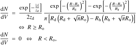 which is the same as Eq. (1) of
Mottram et al. (2011), normalized in such a
way that
which is the same as Eq. (1) of
Mottram et al. (2011), normalized in such a
way that 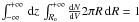 ; here R is the
galactocentric distance, z the height on the Galactic plane,
Ro = 2.2 kpc,
Rd = 6.99 kpc,
Rh = 1.71 kpc, and
zd = 0.039 kpc (from Mottram et al. 2011);
; here R is the
galactocentric distance, z the height on the Galactic plane,
Ro = 2.2 kpc,
Rd = 6.99 kpc,
Rh = 1.71 kpc, and
zd = 0.039 kpc (from Mottram et al. 2011); -
the H ii regions are homogeneous Strömgren spheres ionized by stars with luminosities in the range 103–106 L⊙;
-
the normalized luminosity function (
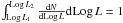 ) of the ionizing star(s) is
described by the power law
) of the ionizing star(s) is
described by the power law  with
L1 = 103 L⊙,
L2 = 106 L⊙,
and β = −0.9, as found by Mottram et al. (2011);
with
L1 = 103 L⊙,
L2 = 106 L⊙,
and β = −0.9, as found by Mottram et al. (2011); -
the normalized electron density distribution (
 ) is also described by a power law,
i.e.,
) is also described by a power law,
i.e., 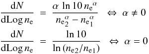 with
ne1 = 30 cm-3 and
ne2 = 2 × 104 cm-3
to span the range of ne in Fig. 5.
with
ne1 = 30 cm-3 and
ne2 = 2 × 104 cm-3
to span the range of ne in Fig. 5.
Under these assumptions, the number of Galactic H ii regions per unit volume,
dex in luminosity, and dex in electron density is given by the expression  (A.1)where NHII is
the total number of H ii regions. There are only two free parameters in this
model: the index α and NHII. To find the
corresponding values, we can fit the electron density function obtained from our data
that is represented by the points with error bars in Fig. A.1. The number of H ii regions in each
ne bin of this figure can be calculated from the model in
the following way. The volume of the Galaxy is divided into a suitable number of cells
in cylindrical coordinates. For each of these, Eq. (A.1) is used to calculate the number of H ii regions
contained in that cell, spanning all luminosities in the range
L1–L2, and with density
falling in the chosen bin. In this process, only cells falling in the region surveyed by
us (i.e., those with 254 < l < 360° and
|b| < 10°) were counted. Moreover, for each L the
corresponding Lyman continuum, NLy, was computed assuming
the relationship for a cluster rather than that for a single star (see Sect. 5.1), as it seems unlikely that H ii regions
with linear diameters up to 3 pc may be ionized by only one star. From
ne and NLy one can calculate
the diameter of the Strömgren H ii region,
DH ii, and the corresponding angular diameter
and radio flux measured in the instrumental beam.
(A.1)where NHII is
the total number of H ii regions. There are only two free parameters in this
model: the index α and NHII. To find the
corresponding values, we can fit the electron density function obtained from our data
that is represented by the points with error bars in Fig. A.1. The number of H ii regions in each
ne bin of this figure can be calculated from the model in
the following way. The volume of the Galaxy is divided into a suitable number of cells
in cylindrical coordinates. For each of these, Eq. (A.1) is used to calculate the number of H ii regions
contained in that cell, spanning all luminosities in the range
L1–L2, and with density
falling in the chosen bin. In this process, only cells falling in the region surveyed by
us (i.e., those with 254 < l < 360° and
|b| < 10°) were counted. Moreover, for each L the
corresponding Lyman continuum, NLy, was computed assuming
the relationship for a cluster rather than that for a single star (see Sect. 5.1), as it seems unlikely that H ii regions
with linear diameters up to 3 pc may be ionized by only one star. From
ne and NLy one can calculate
the diameter of the Strömgren H ii region,
DH ii, and the corresponding angular diameter
and radio flux measured in the instrumental beam.
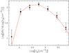 |
Fig. A.1
Electron density function obtained from the data (points with error bars) and best fit from the model (solid line) for α = −0.15 and NHII = 15 000. |
| Open with DEXTER | |
To take into account the bias due to the source selection criteria as well as those introduced by the limited sensitivity of the observations, we took into account only the sources that satisfy the following requirements:
-
L / (4πd2) > 1.6 L⊙ kpc-2, the minimum bolometric flux of the IRAS sources selected by Palla et al. (1991) and Fontani et al. (2005);
-
radio flux above 0.9 mJy beam-1, the mean 3σ sensitivity of our maps;
-
angular diameter below 60′′, the maximum size imaged in our interferometric observations.
The best fit to the electron density function is compared to the data in Fig. A.1. This fit was obtained with
χ2 minimization by varying the two free parameters of the
models over a sufficiently wide range of values. This is illustrated in Fig. A.2, where the χ2 is
plotted as a function of α and NHII. The
thick contour corresponds to the minimum χ2 value (4.64)
plus 2.3, which gives the 1σ confidence level according to Table 1 of
Lampton et al. (1976). We conclude that the best
fit is obtained for NHII =
15 000 and α = −0.15 ± 0.1 As
previously explained, for given ne and
NLy, the H ii region size is univocally
determined. This means that knowledge of the density function
and α = −0.15 ± 0.1 As
previously explained, for given ne and
NLy, the H ii region size is univocally
determined. This means that knowledge of the density function
 provides us also with the analogous
function for the linear diameter,
provides us also with the analogous
function for the linear diameter,  . The latter is shown in Fig. A.3 and compared to the observed distribution.
Clearly, the two are quite consistent for all diameters, with some discrepancy for the
largest DH ii, where the model appears to
overestimate the measured value. However, the largest H ii regions are also the
most difficult to image with an interferometer, and this may explain this small
discrepancy.
. The latter is shown in Fig. A.3 and compared to the observed distribution.
Clearly, the two are quite consistent for all diameters, with some discrepancy for the
largest DH ii, where the model appears to
overestimate the measured value. However, the largest H ii regions are also the
most difficult to image with an interferometer, and this may explain this small
discrepancy.
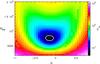 |
Fig. A.2
χ2 obtained by comparing the ne function from the model to that obtained from the data (see Fig. A.1) as a function of the two free parameters, α and NHII. The minimum value (4.64) is obtained for α = −0.15 and NHII = 15 000. The thick contour corresponds to χ2 exceeding the minimum value by 2.3, as recommended by Lampton et al. (1976) to estimate the 1σ confidence level. |
| Open with DEXTER | |
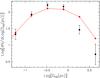 |
Fig. A.3
H ii region diameter function obtained from the data (points with error bars) and from the same model fit (solid line) as in Fig. A.1. |
| Open with DEXTER | |
Appendix B: Figures
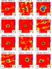 |
Fig. B.1
ATCA continuum images at 18.0 GHz (color scale, units mJy beam-1) and 22.8 GHz (contours). Synthesized beams are indicated at the bottom left (18.0 GHz) and right (22.8 GHz) corners (see Table 1 for values). The primary beam at 22.8 GHz is indicated with the dashed gray circle. When a distance is available, the spatial scale corresponding to 80′′ is indicated at the top of the panel. White stars show the position of water masers (see Table 4). |
| Open with DEXTER | |
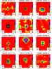 |
Fig. B.1
continued. |
| Open with DEXTER | |
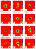 |
Fig. B.1
continued. |
| Open with DEXTER | |
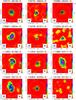 |
Fig. B.1
continued. |
| Open with DEXTER | |
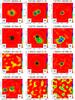 |
Fig. B.1
continued. |
| Open with DEXTER | |
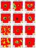 |
Fig. B.1
continued. |
| Open with DEXTER | |
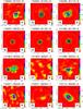 |
Fig. B.1
continued. |
| Open with DEXTER | |
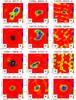 |
Fig. B.1
continued. |
| Open with DEXTER | |
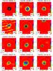 |
Fig. B.1
continued. |
| Open with DEXTER | |
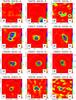 |
Fig. B.1
continued. |
| Open with DEXTER | |
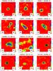 |
Fig. B.1
continued. |
| Open with DEXTER | |
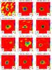 |
Fig. B.1
continued. |
| Open with DEXTER | |
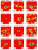 |
Fig. B.1
continued. |
| Open with DEXTER | |
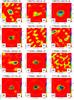 |
Fig. B.1
continued. |
| Open with DEXTER | |
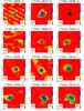 |
Fig. B.1
continued. |
| Open with DEXTER | |
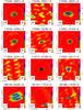 |
Fig. B.1
continued. |
| Open with DEXTER | |
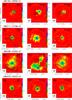 |
Fig. B.2
ATCA, SEST, and MSX maps. For each source we show three panels: left: 21 μm MSX image (color scale) and 1.2 mm SEST image (contours), middle: 1.2 mm SEST image (color scale) and 18.0 GHz ATCA image (contours), and right: 21 μm MSX image (color scale, as in left panel) and 18.0 GHz ATCA image (contours). The spatial scale is shown in sources with distance determination. The primary beam of the ATCA image is shown as a white dashed circle. Water masers are shown as star symbols. |
| Open with DEXTER | |
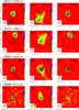 |
Fig. B.2
continued. |
| Open with DEXTER | |
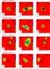 |
Fig. B.2
continued. |
| Open with DEXTER | |
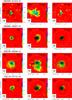 |
Fig. B.2
continued. |
| Open with DEXTER | |
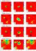 |
Fig. B.2
continued. |
| Open with DEXTER | |
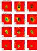 |
Fig. B.2
continued. |
| Open with DEXTER | |
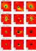 |
Fig. B.2
continued. |
| Open with DEXTER | |
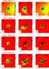 |
Fig. B.2
continued. |
| Open with DEXTER | |
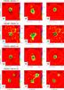 |
Fig. B.2
continued. |
| Open with DEXTER | |
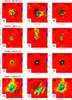 |
Fig. B.2
continued. |
| Open with DEXTER | |
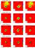 |
Fig. B.2
continued. |
| Open with DEXTER | |
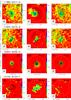 |
Fig. B.2
continued. |
| Open with DEXTER | |
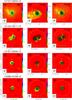 |
Fig. B.2
continued. |
| Open with DEXTER | |
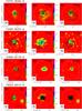 |
Fig. B.2
continued. |
| Open with DEXTER | |
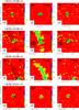 |
Fig. B.2
continued. |
| Open with DEXTER | |
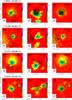 |
Fig. B.2
continued. |
| Open with DEXTER | |
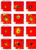 |
Fig. B.2
continued. |
| Open with DEXTER | |
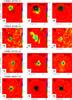 |
Fig. B.2
continued. |
| Open with DEXTER | |
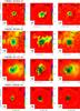 |
Fig. B.2
continued. |
| Open with DEXTER | |
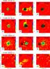 |
Fig. B.2
continued. |
| Open with DEXTER | |
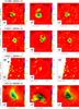 |
Fig. B.2
continued. |
| Open with DEXTER | |
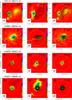 |
Fig. B.2
continued. |
| Open with DEXTER | |
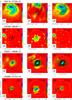 |
Fig. B.2
continued. |
| Open with DEXTER | |
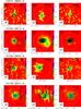 |
Fig. B.2
continued. |
| Open with DEXTER | |
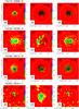 |
Fig. B.2
continued. |
| Open with DEXTER | |
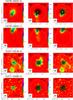 |
Fig. B.2
continued. |
| Open with DEXTER | |
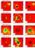 |
Fig. B.2
continued. |
| Open with DEXTER | |
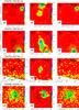 |
Fig. B.2
continued. |
| Open with DEXTER | |
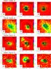 |
Fig. B.2
continued. |
| Open with DEXTER | |
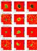 |
Fig. B.2
continued. |
| Open with DEXTER | |
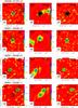 |
Fig. B.2
continued. |
| Open with DEXTER | |
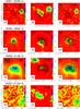 |
Fig. B.2
continued. |
| Open with DEXTER | |
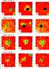 |
Fig. B.2
continued. |
| Open with DEXTER | |
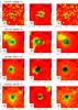 |
Fig. B.2
continued. |
| Open with DEXTER | |
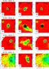 |
Fig. B.2
continued. |
| Open with DEXTER | |
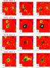 |
Fig. B.2
continued. |
| Open with DEXTER | |
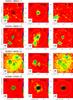 |
Fig. B.2
continued. |
| Open with DEXTER | |
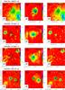 |
Fig. B.2
continued. |
| Open with DEXTER | |
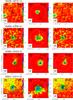 |
Fig. B.2
continued. |
| Open with DEXTER | |
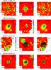 |
Fig. B.2
continued. |
| Open with DEXTER | |
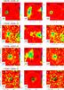 |
Fig. B.2
continued. |
| Open with DEXTER | |
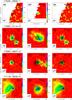 |
Fig. B.2
continued. |
| Open with DEXTER | |
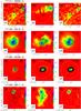 |
Fig. B.2
continued. |
| Open with DEXTER | |
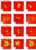 |
Fig. B.2
continued. |
| Open with DEXTER | |
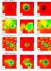 |
Fig. B.2
continued. |
| Open with DEXTER | |
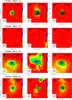 |
Fig. B.2
continued. |
| Open with DEXTER | |
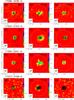 |
Fig. B.2
continued. |
| Open with DEXTER | |
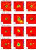 |
Fig. B.2
continued. |
| Open with DEXTER | |
© ESO, 2013
Current usage metrics show cumulative count of Article Views (full-text article views including HTML views, PDF and ePub downloads, according to the available data) and Abstracts Views on Vision4Press platform.
Data correspond to usage on the plateform after 2015. The current usage metrics is available 48-96 hours after online publication and is updated daily on week days.
Initial download of the metrics may take a while.