| Issue |
A&A
Volume 536, December 2011
Planck early results
|
|
|---|---|---|
| Article Number | A22 | |
| Number of page(s) | 24 | |
| Section | Interstellar and circumstellar matter | |
| DOI | https://doi.org/10.1051/0004-6361/201116481 | |
| Published online | 01 December 2011 | |
Planck early results. XXII. The submillimetre properties of a sample of Galactic cold clumps ⋆,⋆⋆
1
Aalto University Metsähovi Radio Observatory, Metsähovintie 114, 02540 Kylmälä, Finland
2
Agenzia Spaziale Italiana Science Data Center, c/o ESRIN, Via Galileo Galilei, Frascati, Italy
3
Astroparticule et Cosmologie, CNRS (UMR7164), Université Denis Diderot Paris 7, Bâtiment Condorcet, 10 rue A. Domon et Léonie Duquet, Paris, France
4
Astrophysics Group, Cavendish Laboratory, University of Cambridge, JJ Thomson Avenue, Cambridge CB3 0HE, UK
5
Atacama Large Millimeter/submillimeter Array, ALMA Santiago Central Offices, Alonso de Cordova 3107, Vitacura, Casilla 763 0355, Santiago, Chile
6
CITA, University of Toronto, 60 St. George St., Toronto, ON M5S 3H8, Canada
7
CNRS, IRAP, 9 Av. colonel Roche, BP 44346, 31028 Toulouse Cedex 4, France
8
California Institute of Technology, Pasadena, California, USA
9
DAMTP, University of Cambridge, Centre for Mathematical Sciences, Wilberforce Road, Cambridge CB3 0WA, UK
10
DSM/Irfu/SPP, CEA-Saclay, 91191 Gif-sur-Yvette Cedex, France
11
DTU Space, National Space Institute, Juliane Mariesvej 30, Copenhagen, Denmark
12
Departamento de Física, Universidad de Oviedo, Avda. Calvo Sotelo s/n, Oviedo, Spain
13
Department of Astronomy and Astrophysics, University of Toronto, 50 Saint George Street, Toronto, Ontario, Canada
14
Department of Earth Sciences and Astronomy, University of Tokyo, Komaba 3-8-1, Meguro, Tokyo 153-8902, Japan
15
Department of Physics & Astronomy, University of British Columbia, 6224 Agricultural Road, Vancouver, British Columbia, Canada
16
Department of Physics, Gustaf Hällströmin katu 2a, University of Helsinki, Helsinki, Finland
17
Department of Physics, Princeton University, Princeton, New Jersey, USA
18
Department of Physics, Purdue University, 525 Northwestern Avenue, West Lafayette, Indiana, USA
19
Department of Physics, University of California, Berkeley, California, USA
20
Department of Physics, University of California, One Shields Avenue, Davis, California, USA
21
Department of Physics, University of California, Santa Barbara, California, USA
22
Department of Physics, University of Illinois at Urbana-Champaign, 1110 West Green Street, Urbana, Illinois, USA
23
Dipartimento di Fisica G. Galilei, Università degli Studi di Padova, Via Marzolo 8, 35131 Padova, Italy
24
Dipartimento di Fisica, Università La Sapienza, P.le A. Moro 2, Roma, Italy
25
Dipartimento di Fisica, Università degli Studi di Milano, Via Celoria, 16, Milano, Italy
26
Dipartimento di Fisica, Università degli Studi di Trieste, Via A. Valerio 2, Trieste, Italy
27
Dipartimento di Fisica,Università di Ferrara, Via Saragat 1, 44122 Ferrara, Italy
28
Dipartimento di Fisica, Università di Roma Tor Vergata, Via della Ricerca Scientifica 1, Roma, Italy
29
Discovery Center, Niels Bohr Institute, Blegdamsvej 17, Copenhagen, Denmark
30
Dpto. Astrofísica, Universidad de La Laguna (ULL), 38206 La Laguna, Tenerife, Spain
31
Eötvös Loránd University, Department of Astronomy, Pázmány Péter sétány 1/A, 1117 Budapest, Hungary
32
European Southern Observatory, ESO Vitacura, Alonso de Cordova 3107, Vitacura, Casilla 19001, Santiago, Chile
33
European Space Agency, ESAC, Planck Science Office, Camino bajo del Castillo s/n, Urbanización Villafranca del Castillo, Villanueva de la Cañada, Madrid, Spain
34
European Space Agency, ESTEC, Keplerlaan 1, 2201 AZ Noordwijk, The Netherlands
35
Helsinki Institute of Physics, Gustaf Hällströmin katu 2, University of Helsinki, Helsinki, Finland
36
INAF - Osservatorio Astrofisico di Catania, Via S. Sofia 78, Catania, Italy
37
INAF - Osservatorio Astronomico di Padova, Vicolo dell’Osservatorio 5, Padova, Italy
38
INAF - Osservatorio Astronomico di Roma, Via di Frascati 33, Monte Porzio Catone, Italy
39
INAF - Osservatorio Astronomico di Trieste, Via G.B. Tiepolo 11, Trieste, Italy
40
INAF/IASF Bologna, Via Gobetti 101, Bologna, Italy
41
INAF/IASF Milano, Via E. Bassini 15, Milano, Italy
42
INRIA, Laboratoire de Recherche en Informatique, Université Paris-Sud 11, Bâtiment 490, 91405 Orsay Cedex, France
43
IPAG (Institut de Planétologie et d’Astrophysique de Grenoble), Université Joseph Fourier, Grenoble 1/CNRS-INSU, UMR 5274, 38041 Grenoble, France
44
Imperial College London, Astrophysics group, Blackett Laboratory, Prince Consort Road, London, SW7 2AZ, UK
45
Infrared Processing and Analysis Center, California Institute of Technology, Pasadena, CA 91125, USA
46
Institut Néel, CNRS, Université Joseph Fourier Grenoble I, 25 rue des Martyrs, Grenoble, France
47
Institut d’Astrophysique Spatiale, CNRS (UMR8617) Université Paris-Sud 11, Bâtiment 121, Orsay, France
48
Institut d’Astrophysique de Paris, CNRS UMR7095, Université Pierre & Marie Curie, 98bis boulevard Arago, Paris, France
49
Institute of Astronomy and Astrophysics, Academia Sinica, Taipei, Taiwan
50
Institute of Astronomy, University of Cambridge, Madingley Road, Cambridge CB3 0HA, UK
51
Institute of Space and Astronautical Science, Japan Aerospace Exploration Agency, 3-1-1 Yoshinodai, Chuo-ku, Sagamihara, Kanagawa, 252-5210, Japan
52 Institute of Theoretical Astrophysics, University of Oslo, Blindern, Oslo, Norway
53
Instituto de Astrofísica de Canarias, C/Vía Láctea s/n, La Laguna, Tenerife, Spain
54
Instituto de Física de Cantabria (CSIC-Universidad de Cantabria), Avda. de los Castros s/n, Santander, Spain
55
Jet Propulsion Laboratory, California Institute of Technology, 4800 Oak Grove Drive, Pasadena, California, USA
56
Jodrell Bank Centre for Astrophysics, Alan Turing Building, School of Physics and Astronomy, The University of Manchester, Oxford Road, Manchester M13 9PL, UK
57
Kavli Institute for Cosmology Cambridge, Madingley Road, Cambridge CB3 0HA, UK
58
LERMA, CNRS, Observatoire de Paris, 61 avenue de l’Observatoire, Paris, France
59
Laboratoire AIM, IRFU/Service d’Astrophysique - CEA/DSM - CNRS - Université Paris Diderot, Bât. 709, CEA-Saclay, 91191 Gif-sur-Yvette Cedex, France
60
Laboratoire Traitement et Communication de l’Information, CNRS (UMR 5141) and Télécom ParisTech, 46 rue Barrault, 75634 Paris Cedex 13, France
61
Laboratoire de Physique Subatomique et de Cosmologie, CNRS/IN2P3, Université Joseph Fourier Grenoble I, Institut National Polytechnique de Grenoble, 53 rue des Martyrs, 38026 Grenoble Cedex, France
62
Laboratoire de l’Accélérateur Linéaire, Université Paris-Sud 11, CNRS/IN2P3, Orsay, France
63
Lawrence Berkeley National Laboratory, Berkeley, California, USA
64
Max-Planck-Institut für Astrophysik, Karl-Schwarzschild-Str. 1, 85741 Garching, Germany
65
MilliLab, VTT Technical Research Centre of Finland, Tietotie 3, Espoo, Finland
66
National University of Ireland, Department of Experimental Physics, Maynooth, Co. Kildare, Ireland
67
Niels Bohr Institute, Blegdamsvej 17, Copenhagen, Denmark
68
Observational Cosmology, Mail Stop 367-17, California Institute of Technology, Pasadena, CA, 91125, USA
69
Optical Science Laboratory, University College London, Gower Street, London, UK
70
SISSA, Astrophysics Sector, Via Bonomea 265, 34136 Trieste, Italy
71
SUPA, Institute for Astronomy, University of Edinburgh, Royal Observatory, Blackford Hill, Edinburgh EH9 3HJ, UK
72
School of Physics and Astronomy, Cardiff University, Queens Buildings, The Parade, Cardiff CF24 3AA, UK
73
Space Sciences Laboratory, University of California, Berkeley, California, USA
74
Spitzer Science Center, 1200 E. California Blvd., Pasadena, California, USA
75
Stanford University, Dept of Physics, Varian Physics Bldg, 382 Via Pueblo Mall, Stanford, California, USA
76
Université de Toulouse, UPS-OMP, IRAP, 31028 Toulouse Cedex 4, France
77
Universities Space Research Association, Stratospheric Observatory for Infrared Astronomy, MS 211-3, Moffett Field, CA 94035, USA
78
University of Granada, Departamento de Física Teórica y del Cosmos, Facultad de Ciencias, Granada, Spain
79
University of Miami, Knight Physics Building, 1320 Campo Sano Dr., Coral Gables, Florida, USA
80
Warsaw University Observatory, Aleje Ujazdowskie 4, 00-478 Warszawa, Poland
Received: 9 January 2011
Accepted: 22 June 2011
Abstract
We perform a detailed investigation of sources from the Cold Cores Catalogue of Planck Objects (C3PO). Our goal is to probe the reliability of the detections, validate the separation between warm and cold dust emission components, provide the first glimpse at the nature, internal morphology and physical characterictics of the Planck-detected sources. We focus on a sub-sample of ten sources from the C3PO list, selected to sample different environments, from high latitude cirrus to nearby (150pc) and remote (2kpc) molecular complexes. We present Planck surface brightness maps and derive the dust temperature, emissivity spectral index, and column densities of the fields. With the help of higher resolution Herschel and AKARI continuum observations and molecular line data, we investigate the morphology of the sources and the properties of the substructures at scales below the Planck beam size. The cold clumps detected by Planck are found to be located on large-scale filamentary (or cometary) structures that extend up to 20pc in the remote sources. The thickness of these filaments ranges between 0.3 and 3pc, for column densities NH2 ~ 0.1 to 1.6 × 1022 cm-2, and with linear mass density covering a broad range, between 15 and 400 M⊙ pc-1. The dust temperatures are low (between 10 and 15K) and the Planck cold clumps correspond to local minima of the line-of-sight averaged dust temperature in these fields. These low temperatures are confirmed when AKARI and Herschel data are added to the spectral energy distributions. Herschel data reveal a wealth of substructure within the Planck cold clumps. In all cases (except two sources harbouring young stellar objects), the substructures are found to be colder, with temperatures as low as 7K. Molecular line observations provide gas column densities which are consistent with those inferred from the dust. The linewidths are all supra-thermal, providing large virial linear mass densities in the range 10 to 300 M⊙ pc-1, comparable within factors of a few, to the gas linear mass densities. The analysis of this small set of cold clumps already probes a broad variety of structures in the C3PO sample, probably associated with different evolutionary stages, from cold and starless clumps, to young protostellar objects still embedded in their cold surrounding cloud. Because of the all-sky coverage and its sensitivity, Planck is able to detect and locate the coldest spots in massive elongated structures that may be the long-searched for progenitors of stellar clusters.
Key words: ISM: clouds / dust, extinction / stars: formation / ISM: structure / submillimeter: ISM / stars: protostars
Appendix A is available in electronic form at http://www.aanda.org
Corresponding author: I. Ristorcelli, e-mail: This email address is being protected from spambots. You need JavaScript enabled to view it.
© ESO, 2011
1. Introduction
The main difficulty in understanding star formation lies in the vast range of scales involved in the process, including not only the gravitationally unstable densest and coldest structures, but also their large-scale environment. The characteristics of star formation, described by the stellar mass distribution, the formation efficiency, the evolutionary timescales, and by the modes of formation (clustered or isolated, spontaneous or triggered) are linked to the properties of the cold cores and those of their Galactic surroundings. Theory predicts that the initial mass function (IMF) is largely determined during the pre-stellar core fragmentation phase, but the latter depends on the properties of the pre-stellar cores, particularly the nature of their support against self-gravity, and their density and temperature distributions. Understanding star formation therefore also requires an understanding of the formation and evolution of dense cores. Turbulence, magnetic fields, and gravity all contribute at sub-parsec scales as well as Galactic scales (see reviews of Bergin & Tafalla 2007; McKee & Ostriker 2007; Ward-Thompson et al. 2007; Crutcher et al. 2009).
So far, ground-based (e.g., Motte et al. 1998; Johnstone et al. 2000) and Herschel (e.g., André et al. 2010; di Francesco et al. 2010; Könyves et al. 2010) observations of nearby star-forming regions have revealed a core mass spectrum with a slope similar to that of the IMF. This intriguing result calls for broader investigations, in particular towards the inner Galaxy, where the Galactic environment differs from that of the Solar neighbourhood, and the star formation efficiency is anticipated to be different.
The physical properties of cold cores are still poorly known, possibly because of the short duration of this phase, but mainly because of observational difficulties. The thermal emission of cold dust, intrinsically weak and blended with that of warmer components, must be sought for in the submillimetre range. A combination of continuum and molecular line studies is also needed to develop a global view of the clouds, from large scales (tens of parsecs) down to the scale of dense cores. During the past decade, the development of sensitive continuum and heterodyne detectors at millimetre and submillimetre wavelengths has significantly increased our knowledge of the properties of the cold dark clouds (see Sect. 1 in Planck Collaboration 2011s,hereafter Paper I). The Planck1 and Herschel satellites now provide a unique opportunity for studying Galactic dust emission and in particular its dense and cold component. The first Herschel surveys have already provided new insights into cold cores, although limited to specific fields (André et al. 2010; Bontemps et al. 2010; Könyves et al. 2010; Men’shchikov et al. 2010; Molinari et al. 2010; Motte et al. 2010; Peretto et al. 2010; Schneider et al. 2010; Stutz et al. 2010; Ward-Thompson et al. 2010; Zavagno et al. 2010).
The Planck satellite (Tauber et al. 2010; Planck Collaboration 2011a) provides complementarity to Herschel by carrying out an all-sky survey that is well suited for the systematic detection of cold cores. In Paper I, we present the first statistical results of the cores from this survey. Combining Planck and IRAS 100 μm data, we have built a preliminary catalogue of 10,783 cold cores (the Cold Core Catalogue of Planck Objects, C3PO). A sub-sample of the most reliable detections is delivered as part of the Planck Early Release Compact Source Catalogue (ERCSC, see Planck Collaboration 2011c), i.e. the Early Cold Cores (ECC) catalogue. The cores from C3PO cover a wide range in properties, with: temperature, from 7K to 19K, with a peak around 13K; density from 102 cm-3 to 105 cm-3, with an average value of 2 × 103 cm-3; mass from 0.4 to 2.4 × 10⁵ M⊙; and size ranging from 0.2 to 18pc. The sources are found to be extended, and more importantly are elongated, with a distribution of aspect ratios extending up to 4 and peaking at twice the beam size of the Planck-HFI instrument. As discussed in Paper I, these properties better match the definition of “clumps” rather than “cores” (see Williams et al. 2000; Bergin & Tafalla 2007). Clumps may contain dense cores, which are likely the precursors of individual or multiple stars. Thus, the main population seen with Planck does not correspond to single pre-stellar cores, but ensembles of cold substructures. A detailed study of the Planck cold objects requires observations at higher resolution. This is the main objective of the Herschel open time key program “Galactic Cold Cores” that is dedicated to following up of a sample of Planck cores.
In this paper we present the first detailed analysis of ten representative sources from the C3PO catalogue. The targets have been selected to cover different types of clump, spanning a wide range of mass, temperature, and density, and located in different environments, ranging from high latitude cirrus to nearby and distant molecular complexes. We combine the Planck data with available ancillary data (in particular IRIS, 2MASS and AKARI) and dedicated follow-up observations with Herschel and ground-based radio telescopes. Using these ancillary data, we seek to confirm the Planck detections and to demonstrate the reliability of the method which used only Planck and IRAS data to determine the source parameters that enter the C3PO catalogue (Paper I) and ECC catalogue (Planck Collaboration 2011c,v). The higher resolution continuum and line data make it possible to examine the internal structure of the Planck sources. They provide the first hints about the process of internal fragmentation and the physical state of the compact cores at scales below the size of the Planck beam. These properties are essential for the interpretation of the full C3PO catalogue and will be a major topic for the projects carrying out follow-up studies of C3PO and ECC catalogue sources.
After describing the observational data set and the source sample selection (Sect. 2), we explain the analysis methods used to derive physical properties for the cores (Sect. 3). The main results are presented in Sect. 4. By fitting spectral energy distributions (SEDs) we derive temperatures, emissivity spectral indices, and column densities for the cores and the surrounding fields, and estimate the linear mass densities, masses and bolometric luminosities of the cores (Sect. 4.1). The small-scale structures within the Planck clumps are studied with the help of Herschel and AKARI data (Sect. 4.3.1), and the gas properties of a few cores are derived from molecular line data (Sect. 4.3.3). Following a discussion of the physical characteristics of the Planck cores, we present our summary and perspectives for the future in Sect. 6.
2. Observations
2.1. The sources
We have selected from the C3PO ten sources with high reliability, signal-to-noise ratio S/N ≥ 8, and low colour temperature, T ≤ 14K (see Paper I). An initial Monte Carlo sampling of the full C3PO catalogue was performed to prepare a candidate list that covered the full range in Galactic position, temperature, flux, and column density. Further selection was made by examining the Planck data and ancillary information from IRIS (Miville-Deschênes & Lagache 2005), 2MASS extinction (Skrutskie et al. 2006), and CO line data from Dame et al. (2001) and NANTEN surveys (e.g., Fukui et al. 1999), as well as IRAS and AKARI point source catalogues and by cross-checking the sources with the SIMBAD database. The selected sources represent different large-scale morphologies and environments, including filaments, isolated and clustered structures and high-latitude cirrus clouds. One key criterion was the knowledge of the source distance, derived either with an extinction method (Marshall et al. 2006), by association with a known molecular cloud complex, or through a kinematic distance estimate (see Paper I). Nine out of the ten sources have already been observed with Herschel as part of the open time key program “Galactic cold cores.” In particular, the sample includes the three targets observed during the Herschel science demonstration phase (SDP, see Juvela et al. 2010, 2011). Half of the sources in the sample are in the Planck ECC. This is mainly due to the criteria used to select the most reliable detections from the C3PO full catalogue (see Paper I): with T < 14K for the colour temperature corresponding to the aperture photometry SED, and a high signal to noise ratio for the source detection (S/N > 15).
The targets are listed in Table 1 and presented in detail in the Appendix. The ten sources that we focus on will hereafter be referred to by the labels S1 through S10.
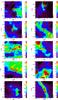 |
Fig.1 Planck-HFI brightness emission maps at 857GHz. The colour scale is in MJysr-1. Note the large dynamic range of the Planck cold clumps from 10MJysr-1 (S2) to 250MJysr-1 (S9). |
Source selection.
2.2. Planck data
Planck (Tauber et al. 2010; Planck Collaboration 2011a) is the third generation space mission to measure the anisotropy of the cosmic microwave background (CMB). It observes the sky in nine frequency bands covering 30–857GHz with high sensitivity and angular resolution from 31′ to 5′. The Low Frequency Instrument (LFI; Mandolesi et al. 2010; Bersanelli et al. 2010; Mennella et al. 2011) covers the 30, 44, and 70GHz bands with amplifiers cooled to 20K. The High Frequency Instrument (HFI; Lamarre et al. 2010; Planck HFI Core Team 2011a) covers the 100, 143, 217, 353, 545, and 857 GHz bands with bolometers cooled to 0.1K. Polarisation is measured in all but the highest two bands (Leahy et al. 2010; Rosset et al. 2010). A combination of radiative cooling and three mechanical coolers produces the temperatures needed for the detectors and optics (Planck Collaboration 2011b). Two data processing centres (DPCs) check and calibrate the data and make maps of the sky (Planck HFI Core Team 2011b; Zacchei et al. 2011). Planck’s sensitivity, angular resolution, and frequency coverage make it a powerful instrument for Galactic and extragalactic astrophysics as well as cosmology. Early astrophysics results are given in Planck Collaboration, 2011h–w.
We use data from the Planck-HFI bands at 857GHz, 545GHz and 353GHz that cover the main peak of the cold dust emission. By restricting ourselves to these highest frequencies, we can perform the analysis at the best angular resolution provided by Planck, i.e., ~4.5′ full width at half-maximum (FWHM).
Figure 1 displays the 857GHz surface brightness maps for each 1° × 1° field. The cores are located at the centres of the maps and show dust emission that ranges from 10 to 220 MJysr-1. They are embedded in extended structures whose shape varies from large filaments (S4, S5, S6, S7 and S10) to more isolated and apparently compact morphologies. Most cores are extended and elongated compared to the Planck beam. As discussed in Paper I, the ellipticity and extension of the cores are not biased by the local beam shape. As an illustration, Fig. A.5 shows the comparison between the local Point Spread Function provided by the FEBeCoP tool (Mitra et al. 2011) with the elliptical Gaussian fit of the sub-sample detections. Typical sizes are from 0.2 to 11pc. Some cores (S2, S8, and S9) are located near bright, warmer regions, where the intensities are higher by up to a factor of 10. In a few cases, the environment exhibits sharp edges, at large scale (see in particular S1, S3 and S7).
The full set of HFI maps (1° × 1° fields from 857 to 100GHz) for each source are shown in Figs. A.1–A.3. These maps have been derived from the HEALPix sky maps (Górski et al. 2005). With the exception of source S2, the cold source at the centre of the maps is usually visible down to 143GHz. At 100GHz the sources become difficult to detect because of the falling intensity of the dust spectrum. Only the Musca filament is clearly visible even at 100GHz, although the surface brightness of the source is low (~0.15 MJysr-1).
Comparison with the 100 μm maps from IRIS (Miville-Deschênes & Lagache 2005) confirms the conclusion of previous submillimetre surveys (using PRONAOS, Archeops, BLAST, and ground-based telescopes) that the cold dust emission is not traced by the 100 μm data, but must be studied using longer wavelengths. The IRIS maps are dominated by the warmer and more extended structure around the cores. This is the basis of the source detection method CoCoCoDeT (Cold Core Colour Detection Tool), that was described in detail in Montier et al. (2010) and in Paper I (Sect. 2.4). It uses as a template the spectrum of the warm emission component estimated from the IRIS 100 μm map. Subtraction of the warm component results in residual maps of the cold emission component from which source fluxes are derived. The detection process is applied independently to the 857, 545, and 353 GHz maps, after smoothing HFI and IRIS data to the same angular resolution of 4.5′. The main steps of the method and the core extraction process are illustrated in the Appendix (in Fig. A.4) for S1. The residual 100 μm signal that remains when a background model is subtracted from the IRIS map (see Paper I) is still needed to constrain the temperature of the cold core SEDs, which typically peak in the range 200–300 μm. The analysis of Sect. 4 will also test the accuracy of this procedure. The coordinates, distances, fluxes densities, and sizes of the selected Planck cores are given in Table 1. The values listed there are taken directly from the C3PO catalogue (see Paper I and Sect. 3.1).
2.3. Herschel observations
The Herschel photometric observations were carried out with the PACS and SPIRE instruments (Pilbratt et al. 2010; Poglitsch et al. 2010; Griffin et al. 2010). Three fields, S8, S9, S10 (corresponding to the source names PCC249, PCC288, and PCC550) were observed in November and December 2009 as part of the Herschel SDP. The other fields were observed between July and September 2010. Most observations were performed separately with PACS (100 and 160 μm) and with SPIRE (250, 350 and 500 μm) in scan mapping mode. Because of the larger field size, S5 and S9 were observed in parallel mode using both instruments simultaneously. The observations employed two orthogonal scanning directions, except for the PACS observations of PCC288 where three scanning directions were used. The data were reduced with Herschel interactive processing environment (HIPE), using the official pipeline with the addition of specialised reduction routines to take advantage of the orthogonal scans for deglitching PACS data and to remove SPIRE scan baselines. The PACS maps were created using the MADmap algorithm (Cantalupo et al. 2010). The SPIRE maps are the product of direct projection onto the sky and averaging of the time ordered data, with a baseline correction.
As for most bolometer observations without an absolute calibrator, the zero level (or offset) of the PACS and SPIRE data are arbitrary. We therefore compared the Herschel and PACS data with the predictions of a model constrained by the Planck and IRAS data. The model uses the all-sky dust temperature maps described in Planck Collaboration (2011o) to infer the average radiation field intensity for each pixel at the common resolution level for the Planck and IRAS data. The DUSTEM model (Compiègne et al. 2010) with the above value for the radiation field intensity was used to predict the expected brightness in the Herschel-SPIRE and PACS bands, using the nearest available Planck or IRAS band for normalisation and taking into account the appropriate colour correction in the Herschel filters. The predicted brightness was correlated with the observed maps smoothed to the Planck and IRAS resolution over the region observed with Herschel and the gain and offsets were derived from this correlation. We have used these gain and offset inter-calibration values in order to convert the maps from Jybeam-1 and Jypix-1 (SPIRE and PACS, respectively) into brightness units (MJysr-1).
2.4. AKARI observations
The AKARI satellite (Murakami et al. 2007) has conducted all-sky surveys at infrared wavelengths centred at 9 μm, 18 μm, 65 μm, 90 μm, 140 μm, and 160 μm. We use the observations made by the FIS instrument in the wide far-infrared bands of 90 μm and 140 μm. The accuracy of the calibration is currently estimated to be 26% at 90 μm and 33% at 140 μm, and the beam sizes of these two bands are ~ 39″ and 58″, respectively. For details of the AKARI far-infrared all sky survey, see Doi et al. (2009).
2.5. Molecular line data
We have carried out “fast” observations of different CO isotopic lines in some 60 Planck cold core candidate fields for the Herschel follow-up programme, five of which are included in the present sample.
The Onsala 20-m telescope was used for 12CO J = 1 → 0, 13CO J = 1 → 0, and C18CO J = 1 → 0 observations in December 2009 and April 2010. An area of a few arcmin in diameter was mapped around the position of the Planck source S3 and the sources in the SDP fields S8 and S9. The observations were carried out in frequency switching mode, with frequency throws of ± 10MHz. The Onsala beam size is approximately ~33″ and the typical rms noise in the 13CO and C18O spectra was below 0.1K per a channel of 0.07 km s-1.
The APEX observations of field S10 were made in July 2010. The size of the 13CO J = 2 → 1 map is ~5′ and the typical rms noise is below 0.2K. The observations were made in position switching mode, using a fixed off position of α = 12h18m58.19s and δ = − 71d42′30.81″ (J2000). The APEX beam size at 220GHz is ~28″.
The IRAM-30m observations were performed in July and October 2010. The EMIR receivers E090 (3mm) and E230 (1mm) were used in parallel with the high resolution correlator (VESPA). The most important parameters for the different settings are given in the Appendix in Table A.1. Maps of 3′ × 3′ were performed using on-the-fly (OTF) mode combined with frequency switching. A summary of the observations and the main results obtained are presented in Sect. 4.3.3.
3. Methods
3.1. Photometry and SEDs
3.1.1. Planck and IRAS photometry
The method for estimating the photometry for the C3PO catalogue has been described in detail in Montier et al. (2010) and Paper I (Sect. 2.4). We recall here only the main steps of the detection and flux extraction process:
-
1.
for each pixel, and for each frequency, the warm backgroundcolour (Cbkg) is estimated as the median value of the ratio of the Planck to 100 μm emission maps (Iν/I100) within a 15′ radius disc;
-
2.
for each Planck frequency, the contribution of the warm component is obtained by extrapolation from 100 μm through
 ;
; -
3.
the cold residual map is computed by subtracting the warm component from the Planck map;
-
4.
the cold source detection is performed using a thresholding method applied on the cold residual map, with the criterion S/N > 4;
-
5.
the source shape is estimated by fitting a 2D elliptical Gaussian to the colour map I857/I100;
-
6.
the flux density at 100 μm is derived by fitting an elliptical Gaussian plus a polynomial surface for the background;
-
7.
the warm template at 100 μm is corrected by removing the source contribution that was estimated in the previous step;
-
8.
aperture photometry at 857, 545, and 353 GHz is performed on the cold residual maps, with the aperture determined by the source shape from step 5.
The photometric uncertainties associated with this method have been estimated with a Monte Carlo analysis (see Paper I, Sect. 2.5); they are 40% for IRAS 100 μm and 8% in the Planck bands. The additional calibration uncertainties to be taken into account are 13.5% and 7%, respectively, for IRIS (Miville-Deschênes & Lagache 2005) and the HFI bands 857, 545, and 353GHz (Planck HFI Core Team 2011b). As described in Paper I, the elliptical Gaussian fit performed in step 5 leads to an estimate of the minor and major axis lengths (σMin and σMaj, respectively), related to the FWHM values, i.e., θMin and θMaj of a Gaussian by  . This method does not include any beam deconvolution. The fluxes and FWHM values are given for each source in Table 1, and the corresponding elliptical fit contours (traced with θMin and θMaj as minor and major axis lengths) are shown in Figs. 3–5.
The 353GHz band includes some contribution from the CO J = 3 → 2 molecular line. The magnitude of this effect has been estimated in Planck HFI Core Team (2011b) using data from 12CO J = 1 → 0 surveys, together with an estimated average line ratio of J = 3 → 2 to J = 1 → 0, and knowledge of the 353GHz band spectral response. The derived correction factor is 171μK in thermodynamic temperature for a CO J = 1 → 0 line area of 1K km s-1. The correction should be small, but the exact effect is hard to estimate for our sources because of the lack of high spatial resolution CO data and because the CO excitation towards cold cores may differ significantly from the average values assumed in deriving the above factor. We therefore present results without making a correction for the CO contribution, but comment on its possible influence later.
3.1.2. Photometry with ancillary data
When using Herschel and AKARI data, the fluxes are estimated at a different resolution and with direct aperture photometry. The maps are convolved to a resolution of 37″ (for Herschel and AKARI 90 μm), 58″ (for Herschel and AKARI 90 μm and 140 μm), or 4.5′ (when including Planck and IRIS data). In each case the aperture has a radius equal to the FWHM of the smoothed data and the background is subtracted using the 30% quantile value within a reference annulus that extends from 1.3 × FWHM to 1.8 × FWHM. In order not to be affected by possible emission from transiently heated grains, the fits employ only data at wavelengths longer than 100 μm. The statistical uncertainty of the flux values is derived from the surface brightness fluctuations in the reference annulus. As above, the calibration uncertainty is taken to be 7% for the Planck channels and 13.5% for IRIS 100 μm. For Herschel we assume a 15% calibration uncertainty for PACS and 12% for SPIRE.
3.2. Estimation of temperatures, spectral indices, and optical depths
Since the dust thermal emission is optically thin in the submillimetre range, the source SEDs can be modelled as a modified blackbody of the form  (1)where Sν is the flux density integrated over the clump solid angle Ωcl (common to all frequencies), τν = NH2μmHκν0(ν/ν0)β is the dust optical depth, and Bν is the Planck function at the dust colour temperature, Tc. Here NH2 is the H2 gas column density, μ = 2.33 the mean mass per particle, mH the mass of the proton, κν0 the mass absorption coefficient at frequency ν0 and β the dust emissivity spectral index. The SED may be rewritten as
 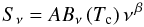 (2)to separate the three quantities (assumed independent) which can be derived from the fit: amplitude A ∝ NH2κν0; spectral index β; and effective temperature Tc. The χ2 minimisation search operates in the (A, Tc, β) space and takes into account the colour corrections for the Planck bands described in Planck HFI Core Team (2011a). In the fitting procedure, we consider only the flux error bars associated with the photometry method, i.e., 40% for IRIS and 8% for HFI bands. In a second step, we compute the final error bars on Tc and β by adding the contribution from calibration uncertainties; these have to be considered separately because the HFI calibration errors are not independent of eachother. In Paper I the size of this effect was estimated using a grid of Tc and β values, and was found to be small ( ≤ 2.5% for Tc and ≤ 2% for β) compared to the uncertainties of the flux extraction method. The final uncertainties in Tc and β are obtained as a quadratic sum of the two contributions. They do not include the correlations between Tc and β inherent in the fitting procedure itself.
Applying the same fitting method pixel by pixel to the IRIS 100 μm and HFI 857, 545, and 353GHz surface brightness images (1° × 1°), we calculate maps of the dust colour temperature and the emissivity index. Here the flux error bars are the quadratic sum of the noise map and the calibration uncertainties. The averaged column densities of the clumps are then derived from the observed flux at ν0 = 857 GHz and the dust colour temperature inferred from the fit: 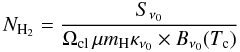 (3)with Ωcl = πσMajσMin.
The value of κν is a main source of uncertainty. Large variations exist between dust models, depending on properties of the dust (see Beckwith et al. 1990; Henning et al. 1995): composition (with or without ice mantles); structure (compact or fluffy aggregates); and size. Both models and observations show that κν increases from the diffuse medium to dense and cold regions by a factor of 3–4 (Ossenkopf & Henning 1994; Kruegel & Siebenmorgen 1994; Stepnik et al. 2003; Juvela et al. 2011; Planck Collaboration 2011u). For this study, we adopt the dust absorption coefficient of Beckwith et al. (1990) inferred for high-density environments (Preibisch et al. 1993; Henning et al. 1995; Motte et al. 1998): 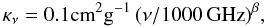 (4)with a fixed emissivity index of β = 2. The reference frequency ν0 = 857GHz chosen to estimate NH2 is such that the extrapolation from 1000GHz with β = 2 (instead of the fitted spectral index) introduces an uncertainty on NH2 of less than 30%. At a distance d, the mass of the clump is simply
  or
or  (5)
(5)
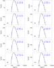 |
Fig. 2 SEDs and fit parameters (T, β) obtained combining Planck HFI and IRIS flux densities integrated over the clump in the cold residual maps. |
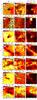 |
Fig. 3 Maps of dust colour temperature, emissivity spectral index and column density for each clump field (the three SDP fields are shown in Juvela et al. (2011) using Herschel maps). The NH2 contours correspond to the ticks on the colour bar. For T and β, the contours are shown respectively at 2K intervals and for β = 1.85. The ellipses trace the FWHMs of the Planck clumps as inferred from the fit (see Table 1). |
4. Results
4.1. Physical parameters derived from Planck and IRIS data
The cold clump SEDs determined using the Planck HFI and IRIS flux densities are shown in Fig. 2. As discussed in Sect. 3.1.1, these SEDs are those of the cold dust residual. The values obtained for the dust temperature and emissivity spectral index are shown in the frames of the figure. Using the method described in Sect. 3.2, we infer the gas column density, bolometric luminosity, and mass of each clump (Table 2). All these parameters (T, β, NH2) are values which are averaged over the line-of-sight and the extent of the cold clumps, which reach the parsec-scale. Denser and/or colder structure is to be expected on smaller scales. These averaged temperatures vary between 10.3 and 14.7K, and the dust emissivity spectral indices range between 1.8 and 2.5.
The column densities are distributed around a mean of 7.5 × 1021 cm-2, with a few of the largest values being above ~1022 cm-2. These relatively moderate column densities also correspond to averaged values over the extent of the clumps. The clumps are likely to be heterogeneous, with denser substructures that will be studied with higher angular resolution data in Sect. 4.3.1. The masses of the sample cover a large range from 3.5 to 1800 M⊙. The highest-mass object, S6, is also the coldest source of the sample, and it is quite extended (~2.9 × 6.7 pc); these properties make this source an interesting candidate for being a high mass star-forming precursor in its early stages. More generally, the sizes of the source sample are rather large, in the range 0.2–11 parsecs, which confirms that they should be better classified as “clumps” rather than “cores,” according to the terminology used for nearby molecular clouds (e.g., Williams et al. 2000; Motte et al. 2007). Scales typically considered for “dense cores” and “clumps” are ~0.1 pc and ~1 pc, respectively.
As noted in Paper I, most of the cold clumps found with the CoCoCoDet procedure are elongated, with aspect ratios significantly larger than unity. The maps of Fig. 1 show that these clumps are not isolated, but are, in many cases, substructures of long filaments, not always straight. Without direct estimates of the density it is difficult to assess that they are actual filaments, denser than their environment. However, their brightness contrast above the background is a few, in the case of S4, S5, S6 and S10, suggesting actual density enhancements given their small thickness. Their length, estimated from their angular size in the maps of Fig. 1 and their distance, ranges from about 5pc for S10 to 18pc for S5.
Because of this, we choose to focus not on the clump mass, that depends on the size of the clump derived from the detection procedure, but on the mass per unit length of the filament at the position of the cold clump. This mass per unit length (or linear mass density) is given by m = 16.7 M⊙ pc-1 N21θMin, where N21 is the clump column density expressed in units of 1021 cm-2 and θMin, the half-power thickness of the clump identified in the Planck maps, is taken as the width of the filament. The linear mass densities are given in Table 2 for all clumps, including those with an aspect ratio only slightly larger than unity. However, they should be considered only as an approximate guide to the linear mass density at the location of the clump.
The linear mass densities vary by a factor ~30 and compare well with those inferred from molecular lines. The range of values (15 to 400 M⊙ pc-1) is characteristic of regions of massive or intermediate-mass star formation, such as Orion and ρ Oph (Hily-Blant et al. 2004). The linear mass densities of the most tenuous filaments (<1 M⊙ pc-1, Falgarone et al. 2001) are not found in the present sub-sample of Planck cold clumps.
Many of the cold clumps detected by Planck therefore appear as cold substructures within larger scale filamentary structures that have length up to ~20 pc in the Planck maps and with parsec-scale thickness (S5, S6, S7). The thinnest filaments found are only a few parsec long and with thickness of a few 0.1pc (S10).
At this stage of the analysis, it is difficult to assess the exact nature of the sources, i.e., discriminating between protostellar objects and starless clumps. We can however use the temperature and bolometric luminosity estimates as first indicators of the evolutionary stage of the sources. Such an approach was proposed by Netterfield et al. (2009) and Roy et al. (2011) in their analysis of the cold cores detected with the balloon-borne experiment, BLAST, in the Cygnus-X and Vela surveys. Among the values obtained for the ratio L/M in our sample (ranging from 0.13 to 0.91 L⊙/ M⊙), it is interesting to note that the three highest (with L/M > 0.6 L⊙/ M⊙) are associated with T > 14K dust sources S2, S8 and S9). As we will see in Sect. 4.3.1, the Planck clumps in these fields harbour warm dust sources, and two of them are associated with young stellar objects.
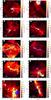 |
Fig.4 Planck 857GHz surface brightness contours on Herschel SPIRE maps at 250 μm. The source S2 has not been observed with Herschel and the displayed image corresponds to the AKARI 90 μm wide filter. As in Fig. 3, the dashed ellipses are tracing the estimated size of the Planck cold clump. |
Clump physical parameters derived from Planck SEDs.
4.2. Colour temperature and spectral index maps
Figure 3 shows the 1° × 1° maps for dust colour temperature and dust spectral index that were estimated using the IRAS 100 μm data and the three highest frequency HFI channels (see Sect. 3.2) without background removal. The three Herschel SDP fields (S8, S9 and S10) are not presented here, because the analysis of T and β was already described in detail in Juvela et al. (2011).
Except for the faint (and not so cold) source S2, a clear signature of cold dust emission is visible directly on these temperature maps at the location of the clumps. The colour temperature characterizing the line-of-sight integrated intensity in the direction of the clump is typically about 14K, warmer by a few Kelvin than the clump temperature deduced from its SED after warm background subtraction. The clumps are embedded within extended structures in the temperature range 16–18K. For reference, dust in the diffuse medium of the local Galactic neighbourhood has a temperature of around 17.5K (Boulanger et al. 1996; Schlegel et al. 1998). In several cases (S4, S5, S6 and S7) the cold clumps appear as the coldest spot (or one of the coldest spots) along filamentary structures, which are already colder than the larger scale environment. The temperature and column density maps are correlated, with the coldest structures corresponding, as expected, to the most opaque parts of the field at the angular resolution probed by Planck. The sharp edges seen in the intensity maps of the fields S1, S3 and S7 are also clearly associated with column density sharp transition. This may be the signature of shock compression and triggering core formation that should be investigated in further studies.
We have compared the results on column densities with extinction measurements. Extinction is calculated with the NICER method (Lombardi & Alves 2001) using stars from the 2MASS catalogue (Skrutskie et al. 2006). The AV maps of the fields are derived assuming an extinction curve that corresponds to RV = 3.1. Preliminary extinction maps are created using nearby fields where IRAS 100 μm data indicates a low dust column density. The AV maps obtained with this method are shown in the Appendix (in Fig. A.6) at 4.5′ resolution. A clear signature is visible, with an increase by about a factor of 2 in AV toward the clumps. The AV values derived (~2–5 mag) are consistent with the previous NH2 estimates of several times 1021 cm-2, derived from the SEDs.
In most fields the colour temperature and the spectral index are seen to be anticorrelated, with high spectral indices being found at the location of the temperature minima. The parameters T and β are known to be connected so that any noise present in the observations tends to produce a similar anticorrelation. However, the spatial coherence of the T and β maps strongly suggests that the results of Fig. 3 are not caused by statistical noise. There is still the possibility of systematic errors, but the similarity of the results obtained in separate fields makes this unlikely. A pure calibration error would change the β and T values in a systematic way but would not significantly affect the dispersion of the spectral index values (Juvela et al. 2011). The line-of-sight temperature variations tend to decrease the observed spectral indices. The effect should be stronger toward the cold clump. The fact that β at those positions is larger than in the diffuse areas suggests that the emissivity index of the grains has increased in the cores more than what is visible in the maps, i.e than that inferred from the line-of-sight integrated SEDs (see Malinen et al. 2011). Therefore, the results support the idea of spatial variation of grain properties that could result from temperature-dependent processes in the dust emission mechanism (Meny et al. 2007; Boudet et al. 2005; Coupeaud et al. 2011, see Paper I discussion). We have estimated the effect of the correction of the CO contribution to the 353 GHz fluxes using the CO data survey from Dame et al. (2001), which covers all sources except S2. This has been performed on the SEDs obtained using the large aperture, which is closer to the angular resolution of the CO data. The results lead to a very small change of the fit parameter values, typically with a ~3% increase of β, and a decrease of the colour temperatures by a few 0.1K.
4.3. Analysis using ancillary data
4.3.1. Herschel and AKARI maps
For all sources we have higher resolution dust continuum data in the form of Herschel (resolution 37″ or better) and/or AKARI (58″ or better) maps. These are used: to examine internal structure of the sources; to derive physical parameters of the Planck sources and compare them with the results of Sect. 4.1; and to study the properties of the structures found at scales below the Planck beam size.
Figure 4 shows Herschel 250 μm data (resolution ~18″) for all, but one, sources. S2 has not been observed with Herschel and we show the AKARI 90 μm map instead (~39″). For comparison, the Planck 857 GHz brightness contours are overplotted and ellipses show the cold clump sizes as derived from elliptical Gaussian fits on the cold residual maps (cf. Paper I and Sect. 3.1.1). A blow-up of the Herschel 250 μm maps is shown in Fig. 5.
In most fields, a significant amount of structure at scales below the Planck resolution is visible. The Musca field (S10) is an exception. The Herschel observations there resolve the filament but do not reveal further structure within the Planck-detected clump. Interestingly, this field is among the closest to the Sun. The other filamentary structures (S4, S5, S6, and S7) break up into numerous smaller bright knots, the brightest often coinciding with the position of the Planck detection. The two cometary shaped clouds (S1 and S3) similarly harbour a number of bright smaller knots and narrow filaments that show up with a large contrast (>2) above an extended background.
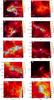 |
Fig. 5 Blow-up of Herschel SPIRE 250 μm maps at the location of the Planck cold clumps localised by their elliptic boundary. The different circles and the annuli refer to the apertures adopted for the photometry used in the SEDs. The large aperture has a 9′ diameter, and the smaller ones correspond to either 74″ (S3 and S5), 116″ (S1, S4, S6, S7, S8 and S9), or 360″ (S10). |
4.3.2. Photometry with Planck, Herschel and AKARI
We have performed fits on the SEDs of selected substructures within the Planck cold clumps to further characterise their inner structure. The aperture photometry is performed after subtraction of a background level estimated as described in Sect. 3. The radius of the largest aperture is 4.5′ (i.e., a diameter of 540″). For the substructures, we use apertures of either 74″ or 116″ diameter. The locations of these apertures are drawn in Fig. 5 and listed in Table 3. The SED fits involve data at wavelengths longer than 100 μm. This removes the problem of a possible contribution from transiently heated grains to the 100 μm flux densities, but also reduces the effects of the line-of-sight temperature variations.
Figure 6 illustrates the various SED estimates for the S1 and S5 fields. It displays the Planck SED as given in the C3PO catalogue (therefore corrected for the warm background contribution) and the aperture photometry using smaller apertures on the brightest substructure of the S1 field (Fig. 5). For the large apertures, the flux densities from Planck and Herschel are in good agreement with each other; in fact it appears that the assumed sources of uncertainty may overestimate the errors. The temperatures obtained for the fixed apertures (Table 3) are the same within the error bars as those derived from the Planck and IRIS data only (Table 2). It is therefore most encouraging that the estimates based only on Planck and IRIS data do not significantly change when the five Herschel bands are added that better cover the short wavelength side of the SED maxima. The modified blackbody parameters derived from the fits are listed in Table 3.
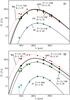 |
Fig.6 Spectral energy distribution of various components in the S1 (upper panel) and S5 (lower panel) fields, including: the Planck SED according to the C3PO catalogue (solid circles and thick solid line), aperture photometry with 270″ and 37″ or 58″ radius aperture sizes (squares and thin solid lines) and the background SED (triangles and dashed line). The temperatures and β values derived from the modified blackbody fits are given in the figure (see also Table 3). The background SED is that of the median surface brightness in the reference annulus surrounding the larger aperture (see Fig. 5). |
One of the most interesting results is the low temperatures obtained for the SEDs in the 74″ apertures. Except for sources S8 and S9, they are all significantly smaller than those obtained in the larger apertures, the lowest values being at about 7K. Therefore, in spite of the large telescope beam size, the sensivity of Planck is such that the cold clump detection method is actually able to pick-up and locate (within a few arcmin) structures of very cold dust that are significantly smaller than the beam.
In sources S8 and S9, the substructures are found to be warmer, with: T ~ 19–21K. As presented in Juvela et al. (2010), the PACS 100 μm maps have revealed the presence of bright compact sources within the Planck-detected clumps. These objects are likely to be very young stellar objects, still embedded in a more extended dense and cold cloud, whose emission is dominating the submillimetre wavelength range studied with Planck. As described in the Appendix, S8 and S9 are both located close to active star-forming regions, with S8 having nearby HII regions, and OB stellar associations.
We note that neither S8 or S9 has any clear counterpart in the 100 μm IRAS map (see Figs. A.2 and A.3); the emission of the young stellar objects is not visible, even although this is the same wavelength as for PACS, probably because the sources are very faint, and diluted with the other components in the IRAS beam. However, for S8, both the 170 μm ISO Serendipity Survey (Stickel et al. 2007) and the AKARI FIS survey at 140 μm (Doi et al. 2009) showed a faint feature at this position. Shorter wavelength data with higher angular resolution would be interesting to combine for these particular sources. Among our sample, the field S8 has been observed by Spitzer, with the 24 μm MIPS data revealing a number of compact sources. Within the Planck clump, the brightest submillimetre peak (PCC288-A in Juvela et al. 2010) is seen to contain at least four distinct mid-infrared sources. These data will be analysed in detail in a future publication.
Results from SED fits based on flux densities from aperture photometry (for data at λ > 100 μm).
We have also estimated the column densities within each aperture, and the average densities and masses obtained in the smallest aperture. In most cases, the derived column densities are higher than those estimated from the Planck clump SEDs. Moreover, as we found with the linear mass densities estimated with Planck data, they vary over a factor of about 30. These values should probably be considered as lower limits, because, as shown in Fig. 5, the annulus associated with the small apertures are close to the source and often include a fraction of signal associated with the source itself. We have estimated the impact of the background level on the derived column density by using the average brightness in the largest annulus instead of the smallest. The derived column densities are increased slightly, by up to a factor of 2.
4.3.3. Analysis of molecular line data
All the Planck clumps observed in 13CO and C18O lines have a clear line detection, and the small maps show peaks that coincide with the cold substructures (Figs. 7 and 8).
The 13CO linewidths (Table 4) are typically 1–2 km s-1 and those of the C18O lines, although narrower, range between 0.3 and 1.6 km s-1. Several velocity components are present, either seen (in a few C18O spectra) as two distinct peaks, or inferred from the non-Gaussian lineshapes, as shown by S6 spectra in Fig. 7. Assuming that the dust and gas in these cold dense clumps is in thermal balance, then the gas temperature is close to 10K and the sound velocity in CO is low, ~0.05 km s-1. The molecular linewidths are therefore all suprathermal. It is interesting to compare the level of non-thermal support provided by these gas motions to the self-gravity. This can be done by comparing the gas linear mass density with its critical (or virial) value, mvir = 2σ2/G which is the largest mass per unit length of a self-gravitating cylinder, given the non-thermal support provided by the internal motions of dispersion σ = Δv/2.35 (Fiege & Pudritz 2000).
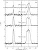 |
Fig.7 CO spectral lines from the Planck clumps S1 and S6 (taken towards the central positions given in Table 1, and with beam apertures in Table A.1. The spectra are in the antenna temperature scale ( |

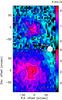 |
Fig.8 The S6 source spectral line intensity maps for C18O J = 1 → 0 (contour steps:0.5K km s-1, top image) and 13CO J = 1 → 0 (contour steps:1K km s-1, bottom image).The white disk indicates the 30-m HPBW size at the 2.7 mm wavelength, valid for both maps. |
The virial linear mass densities inferred from the C18O linewidths of Table 4 range between 10 M⊙ pc-1 for S10, to 260 M⊙ pc-1 for S8. A crude comparison with the linear mass densities estimated at the resolution of the Planck data (Table 2) suggests that the ratios m/mvir are within a factor of a few of unity. Therefore, as a first approximation, these cold clumps are in rough equilibrium between self-gravity and non-thermal support.
The column densities have been estimated from a single line-of-sight towards each object. When available (in the case of IRAM observations), we have combined the J = 1 → 0 and 2 → 1 transitions to derive the excitation temperature and the density using a Large Velocity Gradient radiative transfer model (Goldreich & Kwan 1974). In the case of the Onsala and APEX observations, we only have data for one transition; in these cases, we assume an excitation temperature of 11K and use the C18O line intensity to estimate the column density of the cores. The molecular hydrogen column densities are calculated assuming a C18O fractional abundance of [C18O] / [H2] = 10-7 .
The results are presented in Table 4. The table includes estimates of the mean density, calculated assuming a core size corresponding to a diameter of 74″. The column densities are close to the values derived earlier (Table 3) from the dust continuum data, using the smaller aperture sizes (i.e., 74″ or 116″). The estimated average densities of the cores are only of the order of 103 cm-3, which is lower than the densities found in nearby dense cores (e.g., Myers et al. 1983). The reason for this is that C18O is not a good tracer of dense gas because of the significant degree of CO depletion onto dust grains. Within a cold core, the depletion could be almost complete (e.g., Pineda et al. 2010) and so the investigation of this phenomenon towards the Planck cores is a natural topic for follow-up studies.
CO line parameters for selected lines-of-sight in seven cold core fields.
5. Discussion
5.1. The validity of the cold core detection method
A perhaps unexpected result is the physical size of the Planck detections. They may have been anticipated to be compact point sources, the result of small cores being diluted within the large beam of Planck. However, they are instead found to be significantly extended and elongated, and embedded in filamentary (or cometary) larger-scale structures. As discussed in previous studies, the boundary of a core/clump/cloud structure is always difficult to assess. Curtis & Richer (2010) for instance have shown how much it depends on the method used to identify and extract the core parameters.
In our case, the detection method used to extract sources from the Planck data is based on the colour signature of the objects, designed to enable us to detect the cold residuals after the removal of the warmer background. This results in the discovery of a different, more extended cold component with a more complex morphology than sources found with methods that identify structures on the basis of surface brightness (e.g., the “clumpfind” algorithm of Williams et al. (1994), or a multi-scale wavelet analysis). The high sensitivity of Planck helps to better separate the warm and cold components, particularly in combination with data at somewhat shorter wavelengths.
The faint, mostly filamentary, emission of cold dust that we detect here could perhaps be called a “cold matrix” linking the substructures to each other over a broad range of scales. By combining Planck and Herschel it is possible to probe in detail the link between 10-pc scale filamentary structures and sub-parsec scale cold cores. Future studies with much larger samples should bring new insights to the origin of the cores and the mechanisms associated with their formation.
5.2. The limitations of the SED fitting
One has to be careful not to over-interpret SED fits based on a modified blackbody function, with a single colour temperature and optical depth. In reality the ISM has a broad distribution of dust temperatures and opacities (as well as column densities), within a Planck beam. Shetty et al. (2009) have discussed in detail the biases introduced by line-of-sight temperature variations and noise in the interpretation of such SED fits. Our study suggests that we are not badly contaminated by these effects for several reasons. Firstly Planck’s broad spectral coverage, combined with IRIS allows us to determining both the dust temperature and emissivity spectral index. And secondly, we stress that the cold core detection method identifies structures where the submillimetre SED is dominated by localised dust emission colder than its large scale background.
An indirect indication that the parameters derived from the SEDs fits are not strongly biased is that the physical properties inferred cover the range of values known to be those of pre-stellar cores. Such cores have different properties whether they belong to regions of low- or high-mass star formation. Their column densities range between a few times 1021or 1022 cm-2 in nearby star forming regions (Motte et al. 1998; Kauffmann et al. 2008; Enoch et al. 2006, 2007; Hatchell et al. 2005; Curtis & Richer 2010; André et al. 2010) to ~1023 cm-2 in the cores of infrared dark clouds (IRDCs, Simon et al. 2006; Rathborne et al. 2010; Peretto et al. 2010). These IRDCs, discovered by means of mid-infrared absorption towards the bright background emission of the Galactic Plane (MSX and ISOGAL surveys, Egan et al. 1998; Perault et al. 1996), are thought to be the sites of formation of massive stars and star clusters (Rathborne et al. 2006). The inferred average densities depend on their size, which ranges between < 0.1pc for low-mass dense cores of ~1 M⊙, to 0.5pc or more for ~103 M⊙ IRDC cores. Our Planck cold clumps sub-sample is not located within the MSX IRDCs spatial distribution, so we cannot compare them directly with any IRDC association. However, the properties we derive fall well within this range. It is noteworthy that the Planck cold clumps are elongated structures which tend to exist within extended filaments (up to 30pc in the present subsample), with thickness up to ~3 pc. The IRDCs identified as extinction peaks in mid-infrared maps have similar lengthscales and column densities, but they are usually thinner and therefore have higher densities. It is also interesting that the linear mass densities of the filaments in which the Planck cold clumps are embedded cover the same range as the warm filamentary structures associated with active star-forming regions, i.e., extending up to several 100 M⊙ pc-1.
The temperatures derived in the sample studied here cover a range (10–14.5K) similar to previous estimates on a number of cold condensations detected using multi-wavelength submillimetre observations with the balloon-borne experiments: PRONAOS, T ~ 12 K in star-forming and cirrus regions (Stepnik et al. 2003; Dupac et al. 2003; Bernard et al. 1999); Archeops, 7–18 K (Désert et al. 2008); and BLAST, 9–14K (Netterfield et al. 2009). These temperatures are all lower, however, than those measured in the so-called “quiescent” IRDC cores (Rathborne et al. 2010) that span from 17 to 30K for a similar range in column density (0.3–3 × 1022 cm-2) and mass (10–103 M⊙). The Planck cold clump population may therefore be representative of a still earlier stage of evolution of cold dense cores.
6. Summary and perspectives
We have presented a preliminary analysis of a sample of 10 sources from the C3PO catalogue in order to illustrate and better probe the nature and properties of the cold objects detected with Planck. The sources have been chosen to span a broad range in temperature, density, mass and morphology (inluding filaments and isolated/clustered structures) in a variety of environments, from star-forming regions (both remote and nearby), to high Galactic latitude cirrus clouds. The main findings are as follows:
- 1.
The sources are significantly larger than the Planck beam, with elongated shapes, and appear to belong to filamentary structures, with lengths up to 20pc;
- 2.
The physical parameters of the sources have been derived from SEDs by combining Planck (HFI bands at 857, 545, and 353GHz) and IRIS data, finding T ~ 10−15 K (with a mean value of 12.4K), β ~ 1.8–2.5 (mean 2.2) and NH2 ~ 0.8–16 × 1021 cm-2, from which we infer linear mass densities in the range m = 15–400 M⊙ pc-1, masses M ~ 3.5–1800 M⊙, bolometric luminosities L ~ 1–300 L⊙, and L/M ~ 0.1–0.9 L⊙/ M⊙;
- 3.
Except for the faintest source (which lies at high Galactic latitude), a clear signature of cold dust emission is visible directly in the 1° × 1° maps of dust temperature, spectral index and column density, with colour temperatures of typically ~14 K, surrounded by a warmer extended (often elongated) emission at around 16–18K;
- 4.
Herschel and AKARI observations at higher angular resolution have revealed a rich and complex substructure within the Planck clumps, in most cases the substructures being colder (down to 7K) than the Planck-detected clumps, although in two cases, the substructures are warmer because they harbour compact infrared objects, likely protostellar sources at an early stage;
- 5.
Molecular line observations of 7 of the sources show that all of them are clearly detected in 13CO and C18O, 13CO linewidths typically 1–2 km s-1, and C18O lines always narrower (down to ~0.3 km s-1) but still clearly suprathermal, given the anticipated low temperature of the gas, suggesting that the support of Planck cold clumps against self-gravity is dominated by non-thermal motions.
The first unbiased all-sky catalogue of cold objects provided by Planck offers the opportunity to investigate the properties of the population of Galactic cold objects over the entire sky. The full sample will include objects at the very early stages of evolution, in a variety of large-scale environments, and in particular, outside the well-known molecular complexes, at high latitude or at large distances within the Galactic Plane. For this purpose, dedicated follow-up observations are needed in both higher resolution continuum mode and spectroscopy, which is the objective of the “Galactic Cold Cores” key programme, planning a follow-up with PACS and SPIRE of about 300 Planck cold clumps. In parallel, similar and/or complementary follow-up studies will be possible on the basis of the ECC catalogue which has been delivered to the astronomical community, providing a robust sub-sample of the C3PO catalogue, with more than 900 Planck cold clumps distributed over the whole sky.
Online material
Appendix A: Selected sources, illustration of detection method, source elongation and observational parameters
We list below the main features of the selected fields as known based on previous studies.
S1 lies in a tenuous high-latitude cloud, MCLD 126.5+24.5, located at the border of the Polaris Flare, a large molecular cirrus cloud in the direction of the north celestial pole (Heithausen & Thaddeus 1990), at an estimated distance of 150pc (Bensch et al. 2003). The cloud was first noted from the POSS prints by Lynds (1965) as the small reflection nebula LBN 628. Its cometary globule shape appears similar to what is usually found in active star formation regions, although this nebula is far from any such region. Boden & Heithausen (1993) have studied the gas properties of the densest part of the cloud, observing transition lines of the dense tracors 12CO, 13CO, H2CO, and NH3. The ammonia core (~0.14 pc × 0.07 pc) corresponds to 0.2 M⊙ and a density of 4000 cm-3. Although this density is high compared to the cirrus-like environment, Boden & Heithausen (1993) find that both the cloud and the core are probably gravitationally unbound. The line ratios found are consistent with shocked gas being compressed by the North Celestial Pole Hi loop (Kramer et al. 1998).
S2 is embedded in the tail (~30′ south) of the well-studied cometary globule CG12. This isolated globule is located at high Galactic latitude (l = 316.5°,b = 21.2°), with a 1° long nebular tail nearly perpendicular to the Galactic Plane. Its distance of 550pc has been determined using a photometry-extinction method by Maheswar et al. (2004). Molecular studies using 12CO (van Till et al. 1975; White 1993; Yonekura et al. 1999), C18O (Haikala et al. 2006), H2CO (Goss et al. 1980) and NH3(Bourke et al. 1995) reveal star formation activity, with the presence of a highly collimated bipolar outflow in the head of the cloud. CG12 seems to be a rare example of triggered star formation at relatively large Galactic height (Maheswar et al. 2004).
S3 is located in the constellation of Cassiopeia and has no counterpart in the SIMBAD database. On the sky, the closest Lynds catalogue sources are LDN 1358 and LDN 1355, which are, respectively, at distances of 114 and 118′. These Lynds sources are associated with the Cepheus flare at a distance of 200 ± 50pc (Obayashi et al. 1998; Kauffmann et al. 2008). The Planck detection is associated with an AKARI FIS bright source catalogue source that has a cirrus type spectrum (Yamamura 2008).
S4 is in the Orion region, within a dark cloud that was mapped by Dobashi et al. (2005) in extinction, derived from Digitized Sky Survey images. The source is located six degrees east of the M42 nebula, in the Dobashi et al. cloud 1490, close to its clump P43. It has not been the subject of any dedicated studies, so far. In higher resolution extinction images derived from the colour excess of 2MASS stars, the cloud is seen to reside within a narrow filament. In the Planck data, the filament is clearly visible, but remains unresolved. The source itself is a compact, slightly elongated clump that stands out just as well in the individual Planck frequency maps as in the cold residual map. The Nanten CO data show a peak at the same position, with a line intensity close to 20K km s-1.
S5 is a filamentary structure located near the Vela Molecular Ridge (hereafter VMR), a giant molecular cloud complex in the outer Galaxy. Murphy & May (1991) mapped the VMR in CO, but the mapping did not cover S5. However, Otrupcek et al. (2000) carried out CO observations of the dark cloud DCld 276.9+01.7, with angular extent of 16′ by 3′, and this is interposed on the filament. The detected CO line is rather strong ( K), with a velocity (relative to the local standard of rest) of ~2 km s-1. We derive a kinematic distance for the cloud of ~2 kpc. This is consistent with the distance estimate of the VMR: Liseau et al. (1992) give a photometric distance of (0.7 ± 0.2)kpc for parts A, C and D of the VMR and 2kpc for part B, using the nomenclature established by Murphy & May (1991) and agreeing with their results. Thus we consider it is likely that S5 is part of the VMR. Several studies have been published on the VMR young star-forming region, for example, Olmi et al. (2009) found 141 BLAST cores (starless and proto-stellar) in the Vela-D region.
S6 has been detected in the anti-centre direction (l, b = 176.18, b = −2.11), at a distance estimated to 2kpc using the extinction signature method by Marshall et al. (2006). The filament-shaped core seen with Planck does not coincide with any known object, but is likely associated with the Perseus arm.
S7 has been observed by Ungerechts & Thaddeus (1987) as part of their large CO survey of Perseus, Taurus and Auriga. It is included in their 12th area (see their Table 1), covering 41.8deg2, with a distance of 350pc. For this large region, they estimate a virial mass that is four times higher than the CO mass, showing that this region is out of equilibrium. The Planck source is not associated with any known objects in the SIMBAD database.
S8, S9 and S10 correspond with Herschel SDP sources PCC288, PCC550 and PCC249, respectively. These fields were selected in September 2009 from the cold core detections in the First Light Survey of Planck, in order to perform the first follow-up observations of our Herschel key-program during the Herschel SDP. The fields were mapped with both PACS and SPIRE (with map sizes from 18′ to 50′), and the observations have been described in detail in dedicated papers (Juvela et al. 2010, 2011).
Field S8 is located in Cepheus, at the interface between the Cepheus F molecular cloud (Sargent 1977) and the young stellar group Cep OB3b (Jordi et al. 1996), which is one of the youngest nearby stellar groups. It has been suggestsed that this region could show direct evidence for star formation triggered by the OB association. S9 is an active star formation region close the S140 Hii region. Planck has provided two detections, PCC288-P1 and PCC288-P2 (see Juvela et al. 2010), with the southern source PCC288-P2 being the colder one. The two cores have also been identified in CS J = 1 → 0 mapping of the area by Tafalla et al. (1993). The field S10 is part of the Musca cloud filament, where Planck shows two secure detections of cold cores (T ~ 11 K). The cores have been studied previously in 13CO and C18O by Vilas-Boas et al. (1994).
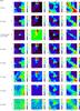 |
Fig. A.1 Multi-band emission maps (in MJy/sr) of the sources S1, S2, S3, and S4. |
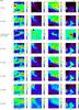 |
Fig. A.2 Multi-band emission maps (in MJy/sr) of the sources S5, S6, S7, and S8. |
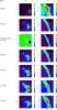 |
Fig. A.3 Multi-band emission maps (in MJy/sr) of the sources S9 and S10. |
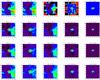 |
Fig. A.4 Illustration of the steps used in the detection and core extraction methods, as applied to source S1. The first column shows the initial surface brightness emission maps in the IRIS and HFI bands. The rows show the process applied to the 100 μm, 857, 545, and 353GHz data, respectively. As described in Paper I, the method follows the following main steps: a “Warm Ref” is built from the IRIS 100 μm map and extrapolated to the Planck bands using the local colour estimated around each pixel of the Planck map (these colour maps are shown in the second column); the “Warm Bkg” map obtained at a given frequency is then removed from the Planck map, revealing the “Cold Residual”; and finally an elliptical Gaussian fit is performed on the colour maps to derive the core size parameters, while aperture photometry is performed on the HFI bands, integrating the signal within the elliptical Gaussian. |
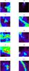 |
Fig. A.5 Comparison of the source elongation with the beam shape determined with the “FEBeCoP” tool (Mitra et al. 2011). The ellipses correspond to the size of the Planck cold clumps derived from the fit; they are plotted at a 2σ level for a better visibility. The dashed circles trace the local beam shape. |
 |
Fig. A.6 Visual extinction maps obtained from 2MASS and the NICER method (cf. Sect. 4.2). The maps are shown at 4.5′ resolution. Contours are drawn at integer values of AV. |
Observational parameters and sensitivity of IRAM observations.
Planck (http://www.esa.int/Planck) is a project of the European Space Agency (ESA) with instruments provided by two scientific consortia funded by ESA member states (in particular the lead countries France and Italy), with contributions from NASA (USA) and telescope reflectors provided by a collaboration between ESA and a scientific consortium led and funded by Denmark.
Acknowledgments
A description of the Planck Collaboration and a list of its members can be found at http://www.rssd.esa.int/index.php?project=PLANCK&page=Planck_Collaboration. The Planck Collaboration acknowledges the support of: ESA; CNES and CNRS/INSU-IN2P3-INP (France); ASI, CNR, and INAF (Italy); NASA and DoE (USA); STFC and UKSA (UK); CSIC, MICINN and JA (Spain); Tekes, AoF and CSC (Finland); DLR and MPG (Germany); CSA (Canada); DTU Space (Denmark); SER/SSO (Switzerland); RCN (Norway); SFI (Ireland); FCT/MCTES (Portugal); and DEISA (EU) This publication makes use of data products from the Two Micron All Sky Survey, which is a joint project of the University of Massachusetts and the Infrared Processing and Analysis Center/California Institute of Technology, funded by the National Aeronautics and Space Administration and the National Science Foundation. This research has made use of the SIMBAD database, operated at CDS, Strasbourg, France. This research is based on observations with AKARI, a JAXA project with the participation of ESA.
References
- André, P., Men’shchikov, A., Bontemps, S., et al. 2010, A&A, 518, L102 [NASA ADS] [CrossRef] [EDP Sciences] [Google Scholar]
- Beckwith, S. V. W., Sargent, A. I., Chini, R. S., & Guesten, R. 1990, AJ, 99, 924 [NASA ADS] [CrossRef] [Google Scholar]
- Bensch, F., Leuenhagen, U., Stutzki, J., & Schieder, R. 2003, ApJ, 591, 1013 [Google Scholar]
- Bergin, E. A., & Tafalla, M. 2007, ARA&A, 45, 339 [NASA ADS] [CrossRef] [Google Scholar]
- Bernard, J. P., Abergel, A., Ristorcelli, I., et al. 1999, A&A, 347, 640 [NASA ADS] [Google Scholar]
- Bersanelli, M., Mandolesi, N., Butler, R. C., et al. 2010, A&A, 520, A4 [NASA ADS] [CrossRef] [EDP Sciences] [Google Scholar]
- Boden, K., & Heithausen, A. 1993, A&A, 268, 255 [NASA ADS] [Google Scholar]
- Bontemps, S., André, P., Könyves, V., et al. 2010, A&A, 518, L85 [NASA ADS] [CrossRef] [EDP Sciences] [Google Scholar]
- Boudet, N., Mutschke, H., Nayral, C., et al. 2005, ApJ, 633, 272 [NASA ADS] [CrossRef] [Google Scholar]
- Boulanger, F., Abergel, A., Bernard, J., et al. 1996, A&A, 312, 256 [NASA ADS] [Google Scholar]
- Bourke, T. L., Hyland, A. R., & Robinson, G. 1995, MNRAS, 276, 1052 [NASA ADS] [Google Scholar]
- Cantalupo, C. M., Borrill, J. D., Jaffe, A. H., Kisner, T. S., & Stompor, R. 2010, ApJS, 187, 212 [NASA ADS] [CrossRef] [Google Scholar]
- Compiègne, M., Flagey, N., Noriega-Crespo, A., et al. 2010, ApJ, 724, L44 [NASA ADS] [CrossRef] [Google Scholar]
- Coupeaud, A., Demyk, K., Meny, C., & Nayral, C. 2011, in IAU Symp., 280, 138 [Google Scholar]
- Crutcher, R. M., Hakobian, N., & Troland, T. H. 2009, ApJ, 692, 844 [NASA ADS] [CrossRef] [Google Scholar]
- Curtis, E. I., & Richer, J. S. 2010, MNRAS, 402, 603 [NASA ADS] [CrossRef] [Google Scholar]
- Dame, T. M., Hartmann, D., & Thaddeus, P. 2001, ApJ, 547, 792 [NASA ADS] [CrossRef] [Google Scholar]
- Désert, F., Macías-Pérez, J. F., Mayet, F., et al. 2008, A&A, 481, 411 [NASA ADS] [CrossRef] [EDP Sciences] [Google Scholar]
- di Francesco, J., Sadavoy, S., Motte, F., et al. 2010, A&A, 518, L91 [NASA ADS] [CrossRef] [EDP Sciences] [Google Scholar]
- Dobashi, K., Uehara, H., Kandori, R., et al. 2005, PASJ, 57, 1 [Google Scholar]
- Doi, Y., Etxaluze Azkonaga, M., White, G., et al. 2009, in The Next-Generation Infrared Space Mission: SPICA, ed. A. M. Heras, B. M. Swinyard, K. G. Isaak, & J. R. Goicoechea, 4018 [Google Scholar]
- Dupac, X., Bernard, J., Boudet, N., et al. 2003, A&A, 404, L11 [NASA ADS] [CrossRef] [EDP Sciences] [Google Scholar]
- Egan, M. P., Shipman, R. F., Price, S. D., et al. 1998, ApJ, 494, L199 [NASA ADS] [CrossRef] [Google Scholar]
- Enoch, M. L., Young, K. E., Glenn, J., et al. 2006, ApJ, 638, 293 [NASA ADS] [CrossRef] [Google Scholar]
- Enoch, M. L., Glenn, J., Evans, II, N. J., et al. 2007, ApJ, 666, 982 [NASA ADS] [CrossRef] [Google Scholar]
- Falgarone, E., Pety, J., & Phillips, T. G. 2001, ApJ, 555, 178 [NASA ADS] [CrossRef] [Google Scholar]
- Fiege, J. D., & Pudritz, R. E. 2000, ApJ, 534, 291 [NASA ADS] [CrossRef] [Google Scholar]
- Fukui, Y., Mizuno, N., Yamaguchi, R., et al. 1999, PASJ, 51, 745 [NASA ADS] [CrossRef] [Google Scholar]
- Goldreich, P., & Kwan, J. 1974, ApJ, 189, 441 [NASA ADS] [CrossRef] [Google Scholar]
- Górski, K. M., Hivon, E., Banday, A. J., et al. 2005, ApJ, 622, 759 [NASA ADS] [CrossRef] [Google Scholar]
- Goss, W. M., Manchester, R. N., Brooks, J. W., et al. 1980, MNRAS, 191, 533 [NASA ADS] [Google Scholar]
- Griffin, M. J., Abergel, A., Abreu, A., et al. 2010, A&A, 518, L3 [Google Scholar]
- Haikala, L. K., Juvela, M., Harju, J., et al. 2006, A&A, 454, L71 [NASA ADS] [CrossRef] [EDP Sciences] [Google Scholar]
- Hatchell, J., Richer, J. S., Fuller, G. A., et al. 2005, A&A, 440, 151 [NASA ADS] [CrossRef] [EDP Sciences] [Google Scholar]
- Heithausen, A., & Thaddeus, P. 1990, ApJ, 353, L49 [NASA ADS] [CrossRef] [Google Scholar]
- Henning, T., Michel, B., & Stognienko, R. 1995, Planet. Space Sci., 43, 1333 [NASA ADS] [CrossRef] [Google Scholar]
- Hily-Blant, P., Falgarone, E., Pineau Des Forêts, G., & Phillips, T. G. 2004, Ap&SS, 292, 285 [Google Scholar]
- Johnstone, D., Wilson, C. D., Moriarty-Schieven, G., et al. 2000, ApJ, 545, 327 [NASA ADS] [CrossRef] [Google Scholar]
- Jordi, C., Trullols, E., & Galadi-Enriquez, D. 1996, A&A, 312, 499 [NASA ADS] [Google Scholar]
- Juvela, M., Ristorcelli, I., Montier, L. A., et al. 2010, A&A, 518, L93 [NASA ADS] [CrossRef] [EDP Sciences] [Google Scholar]
- Juvela, M., Ristorcelli, I., Pelkonen, V.-M., et al. 2011, A&A, 527, A111 [NASA ADS] [CrossRef] [EDP Sciences] [Google Scholar]
- Kauffmann, J., Bertoldi, F., Bourke, T. L., Evans, II, N. J., & Lee, C. W. 2008, A&A, 487, 993 [NASA ADS] [CrossRef] [EDP Sciences] [Google Scholar]
- Könyves, V., André, P., Men’shchikov, A., et al. 2010, A&A, 518, L106 [NASA ADS] [CrossRef] [EDP Sciences] [Google Scholar]
- Kramer, C., Stutzki, J., Rohrig, R., & Corneliussen, U. 1998, A&A, 329, 249 [NASA ADS] [Google Scholar]
- Kruegel, E., & Siebenmorgen, R. 1994, A&A, 288, 929 [NASA ADS] [Google Scholar]
- Lamarre, J., Puget, J., Ade, P. A. R., et al. 2010, A&A, 520, A9 [NASA ADS] [CrossRef] [EDP Sciences] [Google Scholar]
- Leahy, J. P., Bersanelli, M., D’Arcangelo, O., et al. 2010, A&A, 520, A8 [NASA ADS] [CrossRef] [EDP Sciences] [Google Scholar]
- Liseau, R., Lorenzetti, D., Nisini, B., Spinoglio, L., & Moneti, A. 1992, A&A, 265, 577 [NASA ADS] [Google Scholar]
- Lombardi, M., & Alves, J. 2001, A&A, 377, 1023 [NASA ADS] [CrossRef] [EDP Sciences] [Google Scholar]
- Lynds, B. T. 1965, ApJS, 12, 163 [NASA ADS] [CrossRef] [Google Scholar]
- Maheswar, G., Manoj, P., & Bhatt, H. C. 2004, MNRAS, 355, 1272 [NASA ADS] [CrossRef] [Google Scholar]
- Malinen, J., Juvela, M., Collins, D. C., Lunttila, T., & Padoan, P. 2011, A&A, 530, A101 [NASA ADS] [CrossRef] [EDP Sciences] [Google Scholar]
- Mandolesi, N., Bersanelli, M., Butler, R. C., et al. 2010, A&A, 520, A3 [Google Scholar]
- Marshall, D. J., Robin, A. C., Reylé, C., Schultheis, M., & Picaud, S. 2006, A&A, 453, 635 [NASA ADS] [CrossRef] [EDP Sciences] [Google Scholar]
- McKee, C. F., & Ostriker, E. C. 2007, ARA&A, 45, 565 [NASA ADS] [CrossRef] [Google Scholar]
- Mennella, A., Butler, R. C., Curto, A., et al. 2011, A&A, 536, A3 [NASA ADS] [CrossRef] [EDP Sciences] [Google Scholar]
- Men’shchikov, A., André, P., Didelon, P., et al. 2010, A&A, 518, L103 [NASA ADS] [CrossRef] [EDP Sciences] [Google Scholar]
- Meny, C., Gromov, V., Boudet, N., et al. 2007, A&A, 468, 171 [Google Scholar]
- Mitra, S., Rocha, G., Górski, K. M., et al. 2011, ApJS, 193, 5 [NASA ADS] [CrossRef] [Google Scholar]
- Miville-Deschênes, M., & Lagache, G. 2005, ApJS, 157, 302 [NASA ADS] [CrossRef] [Google Scholar]
- Molinari, S., Swinyard, B., Bally, J., et al. 2010, A&A, 518, L100 [NASA ADS] [CrossRef] [EDP Sciences] [Google Scholar]
- Montier, L. A., Pelkonen, V., Juvela, M., Ristorcelli, I., & Marshall, D. J. 2010, A&A, 522, A83 [NASA ADS] [CrossRef] [EDP Sciences] [Google Scholar]
- Motte, F., Andre, P., & Neri, R. 1998, A&A, 336, 150 [NASA ADS] [Google Scholar]
- Motte, F., Bontemps, S., Schilke, P., et al. 2007, A&A, 476, 1243 [NASA ADS] [CrossRef] [EDP Sciences] [Google Scholar]
- Motte, F., Zavagno, A., Bontemps, S., et al. 2010, A&A, 518, L77 [NASA ADS] [CrossRef] [EDP Sciences] [Google Scholar]
- Murakami, H., Baba, H., Barthel, P., et al. 2007, PASJ, 59, 369 [Google Scholar]
- Murphy, D. C., & May, J. 1991, A&A, 247, 202 [NASA ADS] [Google Scholar]
- Myers, P. C., Linke, R. A., & Benson, P. J. 1983, ApJ, 264, 517 [NASA ADS] [CrossRef] [Google Scholar]
- Netterfield, C. B., Ade, P. A. R., Bock, J. J., et al. 2009, ApJ, 707, 1824 [NASA ADS] [CrossRef] [Google Scholar]
- Obayashi, A., Kun, M., Sato, F., Yonekura, Y., & Fukui, Y. 1998, AJ, 115, 274 [NASA ADS] [CrossRef] [Google Scholar]
- Olmi, L., Ade, P. A. R., Anglés-Alcázar, D., et al. 2009, ApJ, 707, 1836 [NASA ADS] [CrossRef] [Google Scholar]
- Ossenkopf, V., & Henning, T. 1994, A&A, 291, 943 [NASA ADS] [Google Scholar]
- Otrupcek, R. E., Hartley, M., & Wang, J. 2000, PASA, 17, 92 [NASA ADS] [CrossRef] [Google Scholar]
- Pagani, L., Daniel, F., & Dubernet, M. 2009, A&A, 494, 719 [NASA ADS] [CrossRef] [EDP Sciences] [Google Scholar]
- Perault, M., Omont, A., Simon, G., et al. 1996, A&A, 315, L165 [NASA ADS] [Google Scholar]
- Peretto, N., Fuller, G. A., Plume, R., et al. 2010, A&A, 518, L98 [NASA ADS] [CrossRef] [EDP Sciences] [Google Scholar]
- Pilbratt, G. L., Riedinger, J. R., Passvogel, T., et al. 2010, A&A, 518, L1 [CrossRef] [EDP Sciences] [Google Scholar]
- Pineda, J. L., Goldsmith, P. F., Chapman, N., et al. 2010, ApJ, 721, 686 [NASA ADS] [CrossRef] [Google Scholar]
- Planck Collaboration 2011a, A&A, 536, A1 [NASA ADS] [CrossRef] [EDP Sciences] [Google Scholar]
- Planck Collaboration 2011b, A&A, 536, A2 [NASA ADS] [CrossRef] [EDP Sciences] [Google Scholar]
- Planck Collaboration 2011c, A&A, 536, A7 [NASA ADS] [CrossRef] [EDP Sciences] [Google Scholar]
- Planck Collaboration 2011d, A&A, 536, A8 [NASA ADS] [CrossRef] [EDP Sciences] [Google Scholar]
- Planck Collaboration 2011e, A&A, 536, A9 [NASA ADS] [CrossRef] [EDP Sciences] [Google Scholar]
- Planck Collaboration 2011f, A&A, 536, A10 [NASA ADS] [CrossRef] [EDP Sciences] [Google Scholar]
- Planck Collaboration 2011g, A&A, 536, A11 [NASA ADS] [CrossRef] [EDP Sciences] [Google Scholar]
- Planck Collaboration 2011h, A&A, 536, A12 [NASA ADS] [CrossRef] [EDP Sciences] [Google Scholar]
- Planck Collaboration 2011i, A&A, 536, A13 [NASA ADS] [CrossRef] [EDP Sciences] [Google Scholar]
- Planck Collaboration. 2011j, A&A, 536, A14 [NASA ADS] [CrossRef] [EDP Sciences] [Google Scholar]
- Planck Collaboration 2011k, A&A, 536, A15 [NASA ADS] [CrossRef] [EDP Sciences] [Google Scholar]
- Planck Collaboration 2011l, A&A, 536, A16 [NASA ADS] [CrossRef] [EDP Sciences] [Google Scholar]
- Planck Collaboration 2011m, A&A, 536, A17 [NASA ADS] [CrossRef] [EDP Sciences] [Google Scholar]
- Planck Collaboration 2011n, A&A, 536, A18 [NASA ADS] [CrossRef] [EDP Sciences] [Google Scholar]
- Planck Collaboration 2011o, A&A, 536, A19 [NASA ADS] [CrossRef] [EDP Sciences] [Google Scholar]
- Planck Collaboration 2011p, A&A, 536, A20 [NASA ADS] [CrossRef] [EDP Sciences] [Google Scholar]
- Planck Collaboration 2011q, A&A, 536, A21 [NASA ADS] [CrossRef] [EDP Sciences] [Google Scholar]
- Planck Collaboration 2011r, A&A, 536, A22 [NASA ADS] [CrossRef] [EDP Sciences] [Google Scholar]
- Planck Collaboration 2011s, A&A, 536, A23 [NASA ADS] [CrossRef] [EDP Sciences] [Google Scholar]
- Planck Collaboration 2011t, A&A, 536, A24 [Google Scholar]
- Planck Collaboration 2011u, A&A, 536, A25 [NASA ADS] [CrossRef] [EDP Sciences] [Google Scholar]
- Planck Collaboration 2011v, The Explanatory Supplement to the Planck Early Release Compact Source Catalogue (ESA) [Google Scholar]
- Planck Collaboration 2011w, A&A, 536, A26 [NASA ADS] [CrossRef] [EDP Sciences] [Google Scholar]
- Planck HFI Core Team 2011a, A&A, 536, A4 [NASA ADS] [CrossRef] [EDP Sciences] [Google Scholar]
- Planck HFI Core Team 2011b, A&A, 536, A6 [NASA ADS] [CrossRef] [EDP Sciences] [Google Scholar]
- Poglitsch, A., Waelkens, C., Geis, N., et al. 2010, A&A, 518, L2 [NASA ADS] [CrossRef] [EDP Sciences] [Google Scholar]
- Preibisch, T., Ossenkopf, V., Yorke, H. W., & Henning, T. 1993, A&A, 279, 577 [NASA ADS] [Google Scholar]
- Rathborne, J. M., Jackson, J. M., & Simon, R. 2006, ApJ, 641, 389 [NASA ADS] [CrossRef] [Google Scholar]
- Rathborne, J. M., Jackson, J. M., Chambers, E. T., et al. 2010, ApJ, 715, 310 [NASA ADS] [CrossRef] [Google Scholar]
- Rosset, C., Tristram, M., Ponthieu, N., et al. 2010, A&A, 520, A13 [NASA ADS] [CrossRef] [EDP Sciences] [Google Scholar]
- Roy, A., Ade, P. A. R., Bock, J. J., et al. 2011, ApJ, 730, 142 [NASA ADS] [CrossRef] [Google Scholar]
- Sargent, A. I. 1977, ApJ, 218, 736 [NASA ADS] [CrossRef] [Google Scholar]
- Schlegel, D. J., Finkbeiner, D. P., & Davis, M. 1998, ApJ, 500, 525 [NASA ADS] [CrossRef] [Google Scholar]
- Schneider, N., Motte, F., Bontemps, S., et al. 2010, A&A, 518, L83 [NASA ADS] [CrossRef] [EDP Sciences] [Google Scholar]
- Shetty, R., Kauffmann, J., Schnee, S., Goodman, A. A., & Ercolano, B. 2009, ApJ, 696, 2234 [NASA ADS] [CrossRef] [Google Scholar]
- Simon, R., Rathborne, J. M., Shah, R. Y., Jackson, J. M., & Chambers, E. T. 2006, ApJ, 653, 1325 [NASA ADS] [CrossRef] [Google Scholar]
- Skrutskie, M., Cutri, R., Stiening, R., et al. 2006, AJ, 131, 1163, owner: marshall Added to JabRef: 2008.07.29 [NASA ADS] [CrossRef] [Google Scholar]
- Stepnik, B., Abergel, A., Bernard, J., et al. 2003, A&A, 398, 551 [NASA ADS] [CrossRef] [EDP Sciences] [Google Scholar]
- Stickel, M., Krause, O., Klaas, U., & Lemke, D. 2007, A&A, 466, 1205 [NASA ADS] [CrossRef] [EDP Sciences] [Google Scholar]
- Stutz, A., Launhardt, R., Linz, H., et al. 2010, A&A, 518, L87 [NASA ADS] [CrossRef] [EDP Sciences] [Google Scholar]
- Tafalla, M., Bachiller, R., & Martin-Pintado, J. 1993, ApJ, 403, 175 [NASA ADS] [CrossRef] [Google Scholar]
- Tauber, J. A., Mandolesi, N., Puget, J., et al. 2010, A&A, 520, A1 [NASA ADS] [CrossRef] [EDP Sciences] [Google Scholar]
- Ungerechts, H., & Thaddeus, P. 1987, ApJS, 63, 645 [NASA ADS] [CrossRef] [Google Scholar]
- van Till, H., Loren, R., & Davis, J. 1975, ApJ, 198, 235 [NASA ADS] [CrossRef] [Google Scholar]
- Vilas-Boas, J. W. S., Myers, P. C., & Fuller, G. A. 1994, ApJ, 433, 96 [NASA ADS] [CrossRef] [Google Scholar]
- Ward-Thompson, D., André, P., Crutcher, R., et al. 2007, Protostars and Planets V, 33 [Google Scholar]
- Ward-Thompson, D., Kirk, J. M., André, P., et al. 2010, A&A, 518, L92 [NASA ADS] [CrossRef] [EDP Sciences] [Google Scholar]
- White, G. J. 1993, A&A, 274, L33 [NASA ADS] [Google Scholar]
- Williams, J. P., de Geus, E. J., & Blitz, L. 1994, ApJ, 428, 693 [NASA ADS] [CrossRef] [Google Scholar]
- Williams, J. P., Blitz, L., & McKee, C. F. 2000, Protostars and Planets IV, 97 [Google Scholar]
- Yamamura, I. 2008, in COSPAR, Plenary Meeting, 37th COSPAR Scientific Assembly, 37, 3529 [Google Scholar]
- Yonekura, Y., Mizuno, N., Saito, H., et al. 1999, PASJ, 51, 911 [NASA ADS] [CrossRef] [Google Scholar]
- Zacchei, A., Maino, D., Baccigalupi, C., et al. 2011, A&A, 536, A5 [NASA ADS] [CrossRef] [EDP Sciences] [Google Scholar]
- Zavagno, A., Russeil, D., Motte, F., et al. 2010, A&A, 518, L81 [NASA ADS] [CrossRef] [EDP Sciences] [Google Scholar]
All Tables
Results from SED fits based on flux densities from aperture photometry (for data at λ > 100 μm).
All Figures
|
Fig.1 Planck-HFI brightness emission maps at 857GHz. The colour scale is in MJysr-1. Note the large dynamic range of the Planck cold clumps from 10MJysr-1 (S2) to 250MJysr-1 (S9). |
| In the text | |
|
Fig. 2 SEDs and fit parameters (T, β) obtained combining Planck HFI and IRIS flux densities integrated over the clump in the cold residual maps. |
| In the text | |
|
Fig. 3 Maps of dust colour temperature, emissivity spectral index and column density for each clump field (the three SDP fields are shown in Juvela et al. (2011) using Herschel maps). The NH2 contours correspond to the ticks on the colour bar. For T and β, the contours are shown respectively at 2K intervals and for β = 1.85. The ellipses trace the FWHMs of the Planck clumps as inferred from the fit (see Table 1). |
| In the text | |
|
Fig.4 Planck 857GHz surface brightness contours on Herschel SPIRE maps at 250 μm. The source S2 has not been observed with Herschel and the displayed image corresponds to the AKARI 90 μm wide filter. As in Fig. 3, the dashed ellipses are tracing the estimated size of the Planck cold clump. |
| In the text | |
|
Fig. 5 Blow-up of Herschel SPIRE 250 μm maps at the location of the Planck cold clumps localised by their elliptic boundary. The different circles and the annuli refer to the apertures adopted for the photometry used in the SEDs. The large aperture has a 9′ diameter, and the smaller ones correspond to either 74″ (S3 and S5), 116″ (S1, S4, S6, S7, S8 and S9), or 360″ (S10). |
| In the text | |
|
Fig.6 Spectral energy distribution of various components in the S1 (upper panel) and S5 (lower panel) fields, including: the Planck SED according to the C3PO catalogue (solid circles and thick solid line), aperture photometry with 270″ and 37″ or 58″ radius aperture sizes (squares and thin solid lines) and the background SED (triangles and dashed line). The temperatures and β values derived from the modified blackbody fits are given in the figure (see also Table 3). The background SED is that of the median surface brightness in the reference annulus surrounding the larger aperture (see Fig. 5). |
| In the text | |
|
Fig.7 CO spectral lines from the Planck clumps S1 and S6 (taken towards the central positions given in Table 1, and with beam apertures in Table A.1. The spectra are in the antenna temperature scale ( |
| In the text | |
|
Fig.8 The S6 source spectral line intensity maps for C18O J = 1 → 0 (contour steps:0.5K km s-1, top image) and 13CO J = 1 → 0 (contour steps:1K km s-1, bottom image).The white disk indicates the 30-m HPBW size at the 2.7 mm wavelength, valid for both maps. |
| In the text | |
|
Fig. A.1 Multi-band emission maps (in MJy/sr) of the sources S1, S2, S3, and S4. |
| In the text | |
|
Fig. A.2 Multi-band emission maps (in MJy/sr) of the sources S5, S6, S7, and S8. |
| In the text | |
|
Fig. A.3 Multi-band emission maps (in MJy/sr) of the sources S9 and S10. |
| In the text | |
|
Fig. A.4 Illustration of the steps used in the detection and core extraction methods, as applied to source S1. The first column shows the initial surface brightness emission maps in the IRIS and HFI bands. The rows show the process applied to the 100 μm, 857, 545, and 353GHz data, respectively. As described in Paper I, the method follows the following main steps: a “Warm Ref” is built from the IRIS 100 μm map and extrapolated to the Planck bands using the local colour estimated around each pixel of the Planck map (these colour maps are shown in the second column); the “Warm Bkg” map obtained at a given frequency is then removed from the Planck map, revealing the “Cold Residual”; and finally an elliptical Gaussian fit is performed on the colour maps to derive the core size parameters, while aperture photometry is performed on the HFI bands, integrating the signal within the elliptical Gaussian. |
| In the text | |
|
Fig. A.5 Comparison of the source elongation with the beam shape determined with the “FEBeCoP” tool (Mitra et al. 2011). The ellipses correspond to the size of the Planck cold clumps derived from the fit; they are plotted at a 2σ level for a better visibility. The dashed circles trace the local beam shape. |
| In the text | |
|
Fig. A.6 Visual extinction maps obtained from 2MASS and the NICER method (cf. Sect. 4.2). The maps are shown at 4.5′ resolution. Contours are drawn at integer values of AV. |
| In the text | |
Current usage metrics show cumulative count of Article Views (full-text article views including HTML views, PDF and ePub downloads, according to the available data) and Abstracts Views on Vision4Press platform.
Data correspond to usage on the plateform after 2015. The current usage metrics is available 48-96 hours after online publication and is updated daily on week days.
Initial download of the metrics may take a while.