| Issue |
A&A
Volume 531, July 2011
|
|
|---|---|---|
| Article Number | A26 | |
| Number of page(s) | 14 | |
| Section | Stellar structure and evolution | |
| DOI | https://doi.org/10.1051/0004-6361/201116686 | |
| Published online | 06 June 2011 | |
High-mass star formation at high luminosities: W31 at >106 L⊙⋆,⋆⋆
1
Max Planck Institute for Astronomy, Königstuhl 17, 69117 Heidelberg, Germany
e-mail: beuther@mpia.de
2
Max Planck Institute for Radioastronomy, Auf dem Hügel 69, 53121 Bonn, Germany
3
I. Physikalisches Institut der Univ. zu Köln, Zülpicher Str. 77, 50937 Köln, Germany
4
Korea Astronomy & Space Science Institute, 776 Daedeokdaero, Yuseong-gu, Daejeon 305-348, Korea
Received: 9 February 2011
Accepted: 9 April 2011
Context. High-mass star formation has been a very active field over the past decade; however, most studies have targeted regions of luminosities between 104 and 105 L⊙. In contrast to that, the highest mass stars reside in clusters exceeding 105 or even 106 L⊙.
Aims. We want to study the physical conditions associated with the formation of the highest mass stars.
Methods. To do this, we selected the W31 star-forming complex with a total luminosity of ~ 6 × 10⁶ L⊙ (comprised of at least two subregions) for a multiwavelength spectral line and continuum study covering wavelengths from the near- and midinfrared via (sub)mm wavelength observations to radio data in the cm regime.
Results. While the overall structure is similar among the multiwavelength continuum data, there are several intriguing differences. The 24 μm emission stemming largely from small dust grains tightly follows the spatial structure of the cm emission tracing the ionized free-free emission. As a result, warm dust resides in regions that are spatially associated with the ionized hot gas (~104 K) of the Hii regions. Furthermore, we find several evolutionary stages within the same complexes, ranging from infrared-observable clusters, via deeply embedded regions associated with active star formation traced by 24 μm and cm emission, to at least one high-mass gas clump devoid of any such signature. The 13CO(2–1) and C18O(2–1) spectral line observations reveal kinematic breadth in the entire region with a total velocity range of approximately 90 km s-1. Kinematic and turbulent structures are set into context. While the average virial mass ratio for W31 is close to unity, the line width analysis indicates large-scale evolutionary differences between the southern and northern subregions (G10.2-0.3 and G10.3-0.1) of the whole W31 complex. A color − color analysis of the IRAC data also shows that the class II sources are broadly distributed throughout the entire complex, whereas the Class 0/I sources are more tightly associated with the active high-mass star-forming regions. The clump mass function – tracing cluster scales and not scales of individual stars – derived from the 875 μm continuum data has a slope of 1.5 ± 0.3, consistent with previous cloud mass functions.
Conclusions. The highest mass and luminous stars form in highly structured and complex regions with multiple events of star formation that do not always occur simultaneously but in a sequential fashion. Warm dust and ionized gas can spatially coexist, and high-mass starless cores with low-turbulence gas components can reside in the direct neighborhood of active star-forming clumps with broad linewidths.
Key words: stars: formation / stars: early-type / stars: individual: W31 / stars: evolution / stars: massive
Tables 1 and 2 are available in electronic form at http://www.aanda.org
13CO, C18O and continuum data are only available at the CDS via anonymous ftp to cdsarc.u-strasbg.fr (130.79.128.5) or via http://cdsarc.u-strasbg.fr/viz-bin/qcat?J/A+A/531/A26
© ESO, 2011
1. Introduction
High-mass star formation research has made significant progress over the past decade from both theoretical and observational points of view. For recent reviews covering various aspects of high-mass star formation, we refer to, e.g., Beuther et al. (2007), Zinnecker & Yorke (2007), Bonnell et al. (2007), McKee & Ostriker (2007) and Krumholz & Bonnell (2007). Unfortunately, because of statistical selection effects and general low-number statistics at the high-luminosity end of the cluster distribution, one observational drawback so far has been that most (sub)mm studies of young high-mass star-forming regions targeted sites of ≤ 105 L⊙, thus stars of mostly less than 30 M⊙ (e.g., Molinari et al. 1996; Plume et al. 1997; Sridharan et al. 2002; Mueller et al. 2002; Fontani et al. 2005). However, some notable exceptions exist, e.g., G10.6-0.4 (Keto 2002), G31.41+0.31 (Cesaroni et al. 1994) or W49 (Homeier & Alves 2005). We therefore lack solid observational constraints on the physical and chemical conditions of young high-mass star-forming regions forming the most luminous and high-mass stars within our Galaxy. In an effort to overcome these limitations, we selected one of the most luminous (~6 × 10⁶ L⊙) but not too distant (~6 kpc compared to, e.g., ~11.4 kpc for W49) giant molecular cloud/high-mass star formation complex G10.2/G10.3 (also known as W31) for a detailed multiwavelength investigation based on APEX 13CO and C18O mapping observations, the 875 μm ATLASGAL continuum survey (Schuller et al. 2009), Spitzer GLIMPSE/MIPSGAL midinfrared data (Churchwell et al. 2009; Carey et al. 2009), and previously published cm continuum data (Kim & Koo 2002).
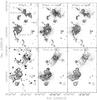 |
Fig. 1 Continuum images of the W31 region. The shown wavelengths are marked in each panel. The 875 μm data are contoured in 3σ steps from 3 to 12σ and continue in 15σ steps from 15σ onwards (1σ ≈ 70 mJy beam-1). The 21 cm image is contoured in 3σ steps from 3 to 12σ (1σ ≈ 5 mJy beam-1), continuing in 0.24 Jy beam-1 steps from 0.12 to 0.84 beam-1, and then go on in 0.48 beam-1 steps. The 24 μm map is saturated toward the peak positions. In the top-left panel the 3-pointed stars mark the position of an O-star by (Bik et al. 2005) and the approximate center of the southern infrared-cluster discussed by Blum et al. (2001). The two white 5-pointed stars show the positions of UCHii regions (Wood & Churchwell 1989). The ellipse marks the emission that velocity-wise is associated with cloud complexes outside our field of view (Sect. 3.2). A scalebar is shown in the top-left panel. The 875 μm and 21 cm beam sizes are shown in the top-right corners of the top-left and bottom-left panels, respectively. In the bottom-left panel, the triangles and stars show IRAC-identified protostellar class 0/I (the two classes are combined) and class II candidates, respectively, following Allen et al. (2004); Megeath et al. (2004); Qiu et al. (2008). |
The high-mass star formation complex W31 contains the subregions G10.2-0.3 and G10.3-0.1, that have already been identified as Hii regions and IRAS sources (IRAS 18064-2020 and IRAS 18060-2005) with high luminosities (e.g., Woodward et al. 1984; Ghosh et al. 1989). Its distance is much debated, and literature values vary between 6 kpc (Wilson 1974; Downes et al. 1980), 14.5 kpc (Corbel et al. 1997) and 3.4 kpc (Blum et al. 2001). The two main regions are separated by approximately 15′ (Fig. 1). At an assumed distance of 6 kpc, the total luminosity and gas mass of the region amounts to ~6 × 10⁶ L⊙ and ~6 × 10⁵ M⊙ (Kim & Koo 2002), respectively. The individual luminosities of the main far-infrared peaks of the two subregions G10.2-0.3 and G10.3-0.1 are estimated to be ~8 × 10⁵ L⊙ and ~6 × 10⁵ L⊙, respectively (Ghosh et al. 1989). Within the largerscale Hii regions, two ultracompact Hii regions were identified, G10.15-0.34 and G10.30-0.15 (Wood & Churchwell 1989). The luminosities of these two UCHiis based on IRAS data are ~1.5 × 10⁶ L⊙ and ~7 × 10⁵ L⊙, respectively (Wood & Churchwell 1989), consistent within a factor 2 with the estimates from Ghosh et al. (1989). It is interesting to note that the infrared clusters in both regions (G10.2-0.3 and G10.3-0.1) are spatially offset from the UCHii regions, indicating different episodes of high-mass star formation. Furthermore, Walsh et al. (1998) identified four distinct Class ii CH3OH maser positions toward the northern G10.3-0.1 subregion also known as IRAS 18060-2005) but none toward the southern G10.2-0.3 subregion (a.k.a. IRAS 18064-2020).
While small submm continuum maps of individual clumps within each of the regions had been obtained over the last few years (e.g., the SCAMPS project, Thompson et al. 2006), there did not exist (sub)mm continuum data encompassing the whole GMC complex. With the advent of the 875 μm survey of the southern Galactic plane (ATLASGAL, Schuller et al. 2009), we now have a complete census of the submm continuum emission of this large-scale star-forming region. Kim & Koo (2002) mapped the whole region in 13CO(1–0) and CS(2–1) at a relatively low spatial resolution of 60′′. They reveal many interesting large-scale features (e.g., that G10.2 and G10.3 may be located on a shell-like structure). Similarly, Zhang et al. (2005) observed the complex in C18O(1–0) with a poor grid separation of 1′. All these studies are not resolving the small-scale structure, and they are not sensitive to the higher-density gas components.
2. Observations and archival data
The C18O(2–1) and 13CO(2–1) data at 219.560 GHz and 220.399 GHz were observed simultaneously with the Atacama Pathfinder Experiment (APEX1, Güsten et al. 2006) in July 2009 in the 1 mm band over the entire W31 complex in the on-the-fly mode. The APEX1 receiver of the SHeFI receiver family has receiver temperatures of ~130 K at the given frequency (Vassilev et al. 2008), and the average system temperatures during the observations were ~250 K. Two Fast-Fourier-Transform-Spectrometer (FFTS, Klein et al. 2006) were connected covering ~2 GHz bandwidth between 219 and 221 GHz with a spectral resolution of ~0.17 km s-1. The data were resampled to 1 km s-1 spectral resolution and converted to main beam brightness temperatures Tmb with forward and beam efficiencies at 220 GHz of 0.97 and 0.82, respectively (Vassilev et al. 2008). The average 1σ rms of the final spectra is ~0.98 K in Tmb. The OFF-positions is approximately 42′/24′ offset from the center of the field (selected via the Stony Brook Galactic Plane CO survey, Sanders et al. 1986), and it apparently has emission in a velocity regime between 27.5 and 36.5 km s-1 showing up as artificial absorption features in our data (see Sect. 3.2). The FWHM of APEX at the given frequencies is ~27.5′′.
The 875 μm data for the region are from the APEX ATLASGAL survey of the Galactic plane (Schuller et al. 2009). The 1σ rms of the data is ~70 mJy beam-1 and the FWHM ~ 19.2′′. The Spitzer IRAC 3.6, 4.5, 5.8 and 8.0 μm images as well as the MIPS 24 μm are taken from the GLIMPSE and MIPSGAL Galactic plane surveys respectively (Churchwell et al. 2009; Carey et al. 2009). Furthermore, we employ the 21 cm radio continuum observations with a spatial resolution of ~37′′ × 25′′ first published by Kim & Koo (2002).
3. Results
3.1. Multiwavelength continuum imaging
3.1.1. General properties
Figure 1 shows a compilation of the different continuum datasets analyzed in this work ranging from the midinfrared with IRAC 8 μm and 24 μm data, to the submm regime at 875 μm and then to radio wavelengths at 21 cm. In a simplified picture, we selected the midinfrared images to trace warm dust emission, the submm data to study cold dust emission, and the cm observations to investigate the ionized gas components. We clearly identify the large-scale structure of the two star formation and Hii region complexes G10.2-0.3 in the south and G10.3-0.1 in the north. At all wavelengths the two complexes exhibit significant substructure, probably most strongly recognizable in the 875 μm image. Since we are dealing with two very luminous but already relatively evolved star formation complexes it is not surprising that many emission features are visible at all presented wavelengths. They show ionized gas as well as warm dust emission caused by the luminous O and B stars (Blum et al. 2001; Bik et al. 2005), and furthermore a large amount of cold dust emission from the still existing gas/dust reservoir present in the whole region. While the former signifies that star formation is already ongoing for a considerable amount of time (>105 − 106 yr), the latter shows that the original gas cloud is not yet dispersed and may still allow further accretion.
Furthermore, the 24 μm and 21 cm data spatially resemble each other well, for example the cometary shape of the northern region G10.3-0.1. An even clearer representation of the correlation between 21 cm and 24 μm emission can be achieved if one plots the observed fluxes pixel by pixel. Figure 2 presents such a “scatter plot” correlating all pixels with 24 μm flux above 120 MJy sr-1 (corresponding to the approximate outskirts of the Hii regions) and the 21 cm emission above the 3σ level of ~0.01 Jy beam-1. Only scales that are close to the beam size of the 21 cm observations were correlated (2-pixel steps corresponding to 29′′). This figure outlines the good spatial correlation between warm dust and ionized gas emission over a broad range of fluxes in the W31 complex. Hence warm dust below the sublimation temperature of ~1500 K spatially coexists with much warmer ionized gas of temperatures around 104 K (e.g., Helfand et al. 2006). Recently, Everett & Churchwell (2010) argue that such dust may stem from continuous ablation processes of small cloudlets that have not been entirely destroyed by the Hii region yet. However, the spatial resolution of the 21 cm observations corresponds to linear scales of about ~0.9 pc. At these scales it is also possible that the observed 21 cm/24 μm correlation stems from an interface between the edges of Hii regions and dense dust shells that are just not resolved by the observations. One should keep in mind that the 24 μm band is mainly sensitive to very small, stochastically heated dust grains (e.g., Draine 2003; Carey et al. 2009) and that, therefore, strong 24 μm emission does not necessarily imply high dust column densities.
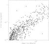 |
Fig. 2 Correlation between 24 μm fluxes and 21 cm fluxes for the W31 complex. Only pixels with 24 μm flux above 120 MJy sr-1 (corresponding to the approximate outskirts of the Hii regions) and 21 cm emission above the 3σ level of ~ 0.01Jy beam-1 are plotted. Furthermore, only correlations on scales of the beam size of the 21 cm observation were used (2-pixel steps corresponding to 29′′). |
While in many cases we see clear associations of emission at different wavelengths, we also witness exactly the contrary. Figure 3 presents a zoom into the northern complex G10.3-0.1, where we also added the near-infrared K-band data from Bik (2004). The latter outline the location of the infrared cluster that is offset from the emission we see at other wavelengths. The O-star marked in Fig. 1 (Bik et al. 2005) is part of that cluster. Directly east of the infrared cluster we find the associated submm clump G10.3E (clump 4 in Table 2) and further to the north G10.3NE (clump 2 in Table 2), both associated with midinfrared, cm and Class ii CH3OH maser emission indicating active star formation. Moving west from the infrared cluster we identify a clear emission peak at all wavelengths (G10.3C in Fig. 3 and clump 1 in Table 2) marking already a relatively evolved part of the UCHii region. Going west, the next source G10.3W1 is still associated with midinfrared, cm continuum and Class ii CH3OH maser emission (G10.3W1 and G10.3W2 merge into clump 6 in the smoothed data of Table 2). Although at a weaker level, this also indicates active high-mass star formation from this gas clump. However, in strong contrast to these subregions, the most western submm peak G10.3W2 in Fig. 3 shows comparably strong submm continuum emission but a complete absence of any 24 μm and 21 cm emission. Thus, this is a high-mass gas clump at a very early evolutionary stage, potentially still in a starless phase prior to any star formation activity. The projected separation of the G10.3W1 and G10.3W2 peak position of ~42′′ corresponds at the assumed distance of 6 kpc still to a projected spatial linear separation of ~1.2 pc. Therefore, each of the submm emission peaks covers scales corresponding to clusters, and therefore each may form a smaller cluster – likely also containing high-mass stars – within the large-scale environment of W31.
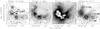 |
Fig. 3 Zoom into the G10.3 complex. In all 4 panels the solid contours present the 875 μm continuum contours (start at 3σ and continue in 9σ steps, 1σ ≈ 70 mJy beam-1) whereas the grey-scale shows other wavelength data as outlined over each panel. The dashed 21 cm contours in the right panel go from 15 to 60 mJy beam-1 in 15 mJy beam-1 steps, and from 120 to 840 mJy beam-1 in 240 mJy beam-1 steps. The K-band data are taken from Bik (2004). The white central part of the 24 μm image is saturated. The triangles in the left panel mark the Class ii CH3OH maser positions from Walsh et al. (1998). The white star in the right panel marks the position of an UCHii region (Wood & Churchwell 1989), and the additional labels there name sources discussed in the main text. |
Figure 1 also shows the distribution of protostellar class 0/I (the two classes are combined) and pre-main-sequence class II sources identified by Spitzer IRAC data based on the selection criteria developed by Allen et al. (2004), Megeath et al. (2004) and Qiu et al. (2008). While the non-detection of any source toward the centers of the two subregions is likely an artifact due to saturation and confusion in these areas, one can tentatively identify a trend that the class 0/I sources are more closely associated with the centers of activity than the class II sources which appear more widely distributed over the field of view. Quantitatively speaking, the mean separations of the northern class 0/I and class II sources from the UCHii region G10.30-0.15 are ~321′′ and ~428′′, respectively, whereas the corresponding mean separations for the southern sources with respect to the UCHii region G10.15-0.34 are ~936′′ and ~1048′′, respectively. These data also indicate that the southern cluster is spatially more distributed and may potentially be already more evolved (see Sect. 4.1).
3.1.2. Clump properties of the 875 μm continuum emission
We can now locate the dense 875 μm gas and dust clumps at a spatial resolution of 19′′, corresponding to linear scales of ~0.5 pc at an assumed distance of 6 kpc. While two of the dense cores are associated with the ultracompact Hii regions G10.15-0.34 and G10.30-0.15 (Fig. 1), there are obviously many dense gas clumps that are promising candidates of ongoing and potentially even younger high-mass star formation. At the given spatial scales of our resolution limit, each submm subsource does not form individual stars but they all should be capable of forming subclusters within the larger-scale region.
To systematically identify gas and dust clumps and to study their properties in such a large and complex region we employ the clumpfind algorithm (Williams et al. 1994) with 3σ contour levels (210 mJy beam-1). With this procedure we identify 73 submm continuum clumps over the entire W31 region (Fig. 4). These clumps are listed in Table 1 with the spatial coordinates of their peak positions, their integrated and peak fluxes, and their linear effective radii reff. Assuming that the submm emission stems from optically thin dust, we can calculate the H2 gas column densities and masses following Hildebrand (1983); Beuther et al. (2002, 2005). Since we do not know the temperature substructure of the entire complex, we use an average dust temperature of 50 K that should be a reasonable proxy for such an active region (e.g., Sridharan et al. 2002). Furthermore, we use a dust grain emissivity index of β = 2 (corresponding to a dust absorption coefficient of κ875 ≈ 0.8 cm2 g-1), and a gas-to-dust mass ratio of 186 is assumed (Jenkins 2004; Draine et al. 2007). Table 1 lists also the derived H2 column densities and masses of the respective gas clumps. With the given uncertainties of temperature and dust composition, we estimate the masses and column densities to be accurate within a factor ~3.
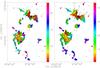 |
Fig. 4 The color-scales show the clump structure and boundaries derived with the automized clumpfind procedure on the original (left) and smoothed (right) 875 μm continuum observations. The contours show the original 875 μm observations with the same contour levels as in Fig. 1. The wedge reflects the clump numbers as in Tables 1 and 2. A few discussed clumps are labeled in the right panel (see also Fig. 11). |
The derived clump masses range between 120 and 8200 M⊙ with a total gas mass in the region of approximately 1.2 × 10⁵ M⊙. The peak column densities vary between 1.5 × 10²² and 3.4 × 1023 cm-2. While the proposed threshold for high-mass star formation of 1 g cm-2 (Krumholz & McKee 2008) corresponds to column densities of ~3 × 1023 cm-2, this does not imply that most clumps are not capable of high-mass star formation, the data clearly show the opposite. In contrast to this, the calculated column densities are measured with a linear beam size of ~0.5 pc, and thus only the average column densities over such area have the derived values. The intrinsic column densities at smaller spatial scales are significantly higher assuming a typical density distribution ∝ r-2 (see also Vasyunina et al. 2009, for similar estimates conducted for infrared dark clouds).
This implies that a large number of the gas clumps in this region should be capable of forming subclusters containing high-mass stars. To estimate how much mass a gas clump needs to have to form a high-mass star, we produce stellar cluster toy-models assuming a star formation efficiency of 30% and an initial mass function (IMF) following Kroupa (2001). To form at least one high-mass star of, e.g., 20 or 40 M⊙, in this scenario the initial gas clumps have to have masses of ~1065 or ~2965 M⊙, respectively. Similar results were recently obtained observationally by Johnston et al. (2009). This clearly indicates that a significant fraction of gas clumps in the W31 region is capable of forming stars in excess of 20 M⊙.
Using the clump masses from Table 1 we also tried to derive a clump mass function ΔN/ΔM ∝ M − α for the region. To overcome fitting artifacts due to different bin sizes, we fitted the data, systematically changing the bin width (see also Rodon et al. 2011). To avoid any sensitivity cutoff we fitted only clumps above 1000 M⊙ and furthermore required at least three non-empty bins. This procedure resulted in 36 fits to the data with different bin sizes each time, allowing us to asses better the error margins of this approach. Figure 5 shows one example fit. While the Poisson errors for each individual fit are relatively large, the combined assessment of all different fits from varying bin sizes in this fitting procedure as well as a comparison to a cumulative fit, allows us to derive a power-law distribution index within reasonable error margins. Our derived power-law index α from this procedure is ~1.5 ± 0.3 (see discussion in Sect. 4.2).
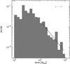 |
Fig. 5 Example clump mass function for the W31 complex for one bin size (here logarithmic bins with 10k ∗ 0.1 < M < 10(k + 1) ∗ 0.1 with k an integer, 36 different bin sizes have been used to overcome fitting artifacts). Only clumps with masses > 1000 M⊙ were used for the fit. |
3.1.3. Smoothed 875 μm data
For a better comparison with the spectral line data discussed in the following section, we also smoothed the 875 μm continuum data to the same spatial resolution as the spectral line observations (~27.5′′). On this smoothed map with a lower rms of 50 mJy beam-1, we again apply the clumpfind algorithm to extract sources, resulting in 44 clumps compared to the 73 clumps in the original data (see Fig. 4 for comparison). For these clumps we also calculated masses and column densities as conducted in the previous section for the un-smoothed data. In addition for comparison purposes with the spectral line data, we also calculate the mass just within the central beams toward each peak position Mpeak. All the parameters extracted for the smoothed clumps are listed in Table 2.
3.2. Kinematics from spectral line data
Star formation processes significantly shape the kinematic and dynamic properties of the molecular gas. While early-on dense starless gas and dust clumps usually exhibit narrow line widths because no (proto)stellar feedback has yet altered the original gas properties, during ongoing star formation, the natal gas clumps are strongly influenced by the central star-forming processes which is reflected in the observable spectral signatures.
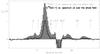 |
Fig. 6 13CO(2–1) and C18O(2–1) (multiplied by a factor 2) spectra averaged over the entire W31 region. The marked velocities show the different velocity regimes used for the 13CO (upper) and C18O (lower) moment maps. |
The 13CO(2–1) and C18O(2–1) observations allow a kinematic analysis of the region. Figure 6 presents the spectra of both species averaged in each case over the entire field of view of the observations. In particular the 13CO(2–1) data show the very broad velocity range present in the region. The figure also marks different velocity regimes used by us to produce moment maps of the data (see below). The velocity regime from 27.5 to 36.5 km s-1 appears in absorption in this averaged spectrum. This, however, is an artifact because we see it in all spectra and hence it stems from emission at this velocity in the OFF position. Interestingly, this velocity range is exactly the same as the velocities we find emission for toward the submm continuum peak marked by an ellipse in Fig. 1. Therefore, this continuum feature in our maps should be associated with other cloud complexes outside of our observed field of view.
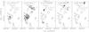 |
Fig. 7 The grey-scale shows different 13CO(2–1) integrated intensity images where the integration regimes are shown in the top of each panel. Contour levels go from 20 to 80% in 20% levels of the respective peak intensities. The dotted contours outline the 875 μm emission at a 3σ level from Fig. 1. |
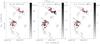 |
Fig. 8 The grey-scale shows C18O(2–1) moment maps: 0th moment or integrated intensity on the left, 1st moment or intensity-weighted velocity in the middle and 2nd moment or intensity-weighted linewidth to the right. The black contours in the left panel show the integrated C18O(2–1) data and go from 20 to 80% in 20% steps. The dotted contours outline the 875 μm emission at a 3σ level from Fig. 1, and the red contours show additionally the high-intensity 875 μm emission in 15σ steps from 15σ onwards (1σ ≈ 70 mJy beam-1). In the right panel, the 3-pointed stars in the north and south mark the position of an O-star by Bik et al. (2005) and the center of the southern cluster discussed by Blum et al. (2001). The 5-pointed stars mark the two UCHii regions (Wood & Churchwell 1989). |
Figure 7 presents 13CO(2–1) integrated intensity images of different parts of the 13CO(2–1) spectrum from Fig. 6. We omit the velocity structure lower than − 6 km s-1 because this is only lower-intensity more diffuse emission that is hard to properly image. However, it very likely belongs to the overall W31 region. The main velocity component present in both W31 complexes (G10.2-0.3 and G10.3-0.1) is the main peak between 2 and 21 km s-1. In contrast to this, the two velocity components between − 6 and 2 km s-1 and 36.5 to 58 km s-1 are clearly only associated with specific subregions within G10.2-0.3 and G10.3-0.1, respectively. As outlined in the previous section, the fact that we see the feature between 27.5 and 36.5 km s-1 not at any other velocity but only as a negative feature throughout the map due to emission from the OFF-position supports the idea that this structure is likely associated with other clouds outside our field of view. Similarly, the structure toward the north between 58 and 77 km s-1 may also not be associated with the W31 region but could be at a different distance. While the main component between 2 and 21 km s-1 is widely distributed, it is difficult to safely distinguish whether the other velocity components in the region are simply chance alignments of projected sources at different distances, or whether there exists an additional (projected) large-scale velocity gradient from blue-shifted emission toward the south-east to more red-shifted emission toward the north-west. As visible in Fig. 6, the averaged C18O(2–1) spectrum exhibits in general similar velocity features as that of 13CO(2–1), however, at a lower level. Therefore, in Fig. 8 we only show the integrated C18O(2–1) emission of the main velocity component between 6 and 19 km s-1.
Figures 8 and 9 present the 0th, 1st and 2nd moment maps (integrated intensity, intensity-weighted velocity structure and intensity-weighted linewidth structure) of the main velocity components of C18O(2–1) and 13CO(2–1), respectively. While the general structure of the 13CO and C18O emission of this main velocity components agrees relatively well with the 875 μm continuum emission, in particular the integrated 13CO(2–1) maps exhibits much more extended gas structure than the dust continuum emission. This is likely a combined effect of the limited sensitivity of the ATLASGAL data on the one hand (approximate rms of 50 mJy beam-1, Schuller et al. 2009), and on the other hand it may also be due to the general large-scale spatial filtering effect inherent to any bolometer observations. Furthermore, the C18O integrated emission spatial structure agrees well with the high column density part of the dust continuum maps outlined by the red contours in Fig. 8.
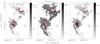 |
Fig. 9 The grey-scale shows different 13CO(2–1) moment maps: 0th moment or integrated intensity on the left, 1st moment or intensity-weighted velocity in the middle and 2nd moment or intensity-weighted linewidth to the right. The black contours in the left panel show the integrated intensity 13CO(2–1) data from 20 to 80% in 20% steps. The dotted contours outline the 875 μm emission at a 3σ level from Fig. 1, and the red contours show additionally the high-intensity 875 μm emission in 15σ steps from 15σ onwards (1σ ≈ 70 mJy beam-1). In the right panel, the 3-pointed stars in the north and south mark the position of an O-star as reported by Bik et al. (2005) and the center of the southern cluster discussed by Blum et al. (2001). The 5-pointed stars mark the two UCHii regions (Wood & Churchwell 1989). |
While some subregions exhibit additional velocity components (see Fig. 7 and discussion above), the 1st moment maps in Figs. 8 and 9 do not exhibit a clear velocity difference between the two large-scale subcomplexes within the main velocity component. Rather in contrast, both regions – G10.2-0.3 and G10.3-0.1 – show velocity substructure associated with the width of the main velocity component. Probably more important, the 2nd moment maps show a very broad distribution of linewidths, extending in 13CO(2–1) to values in excess of 10 km s-1. Although still comparably narrow (see Δv for clump 1 in Tables 1 and 2) in the northern region (G10.3-0.1), the broadest linewidth there is measured toward clump 1 (Table 2), which is spatially associated with the near-infrared cluster around the O-stars (Bik et al. 2005), thus the most evolved part of this subcomplex. Although the southern region G10.2-0.3 exhibits in general much broader line widths compared to the northern region, there the broadest C18O(2–1) and 13CO(2–1) linewidths are attributed again to regions in the close vicinity of the infrared cluster discussed by Blum et al. (2001). Toward the southern and northern regions, the UCHii regions both exhibit comparably broad line width, however, always narrower than toward the gas clumps associated with the infrared clusters.
3.3. Line parameters and virial analysis
In particular the C18O(2–1) spectral line data are suited to a more detailed spectral analysis. Therefore, we extracted the C18O(2–1) spectra toward all peak positions identified by the clumpfind procedure for the dust continuum data. However, one should keep in mind that the spatial resolution of the continuum and line data is different, 19.2′′ and 27.5′′, respectively. While for completeness, we extract the spectra toward all positions from the high-spatial-resolution continuum data (Table 1), for a better comparison, it is more useful to extract the line parameters toward the positions extracted from the smoothed 875 μm continuum map (Sect. 3.1.3). Table 2 lists the derived line parameters toward the smoothed dust continuum peak positions from Gaussian fits to the C18O(2–1) line profiles. Line parameters are peak temperature Tpeak, integrated intensity  , peak velocity vpeak and Full Width Half Maximum line width Δv.
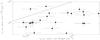 |
Fig. 10 Comparison of H2 column densities derived from the 875 μm dust continuum and C18O(2–1) at the same spatial resolution of 27.5′′. We draw 25% error-bars although the real errors may be even larger as discussed in the main text. The solid line marks the 1:1 relation. |
These line parameters can be used to derive physical quantities, in particular H2 column densities and virial masses. To calculate the C18O and corresponding H2 column densities, we followed the standard local thermodynamic equilibrium (LTE) analysis (Rohlfs & Wilson 2006) assuming optically thin C18O(2–1) emission again at an average temperature of 50 K (Sect. 3.1.2). Comparing individual 13CO and C18O spectra of the region indicates that this assumption is reasonable. The resulting H2 column densities are listed in Tables 1 and 2. While higher/lower temperatures for individual subsources would lower/raise the column density estimates, we use again a uniform temperature to better compare later with the dust continuum derived results (Fig. 10). Non-optically thin C18O emission would also raise the derived column density values.
Furthermore, we calculated virial masses for the given C18O(2–1) line widths following MacLaren et al. (1988)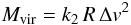 (1)with k2 = 126 for a density profile ρ ∝ r-2, R the radius of the clump defined as half of the FWHM of the beam and Δv the line width given in Table 2. Under the assumption of a flatter density profile (ρ ∝ r-1) or a Gaussian density distribution the virial masses would be approximately factors of 1.5 or 3 higher (MacLaren et al. 1988; Simon et al. 2001). We assume a factor 2 uncertainty for the calculated virial masses. The derived masses are listed also in Tables 1 and 2.
Figure 10 presents a comparison of the H2 column densities derived on the one hand via the 875 μm continuum emission and on the other hand from the C18O(2–1) emission at the same spatial resolution of 27.5′′. Although the real errors may even be larger (see discussions above), for clarity we draw “only” 25% error margins in the figure. For almost all positions, the H2 column densities derived from the 875 μm data exceed those derived via the C18O emission. Even considering the given uncertainties for the different column density derivations, this is plausible since with a critical density of ~ 104 cm-3, C18O(2–1) does not trace the highest density gas and therefore may miss the highest column density regions. Similar results were recently obtained by Walsh et al. (2010) for the regions NGC 6334I & I(N) where even the very optically thin CO isotopologue C17O(1–0) did not trace the dust continuum derived column density peak of the region.
A different comparison is presented in Fig. 11 where we show the gas masses derived from the 875 μm dust continuum peak fluxes Mpeak against the masses obtained from the C18O(2–1) line width under the assumption of virial equilibrium Mvir. Similarly to the column density figure, we draw “only” 25% error margins for clarity reasons. To first order, we find no clear trend but a “scatter plot”. However, excluding clumps 1, 2, 4, 6 and 10 (Fig. 4 and Table 2), although with a considerable scatter most other clumps are located in the vicinity of the Mvir/Mpeak ~ 1 relation. Therefore, many of these clumps may not be far from virial equilibrium. Inspecting clumps 1, 2, 4, 6 and 10 below the 1:1 relation in Fig. 11 in more detail, interestingly we find that all these sources are associated with the northern subregion G10.3-0.1 (Figs. 11, 4 and 3), whereas the southern region G10.2-0.3 is dominated by higher Mvir/Mpeak ratios. Hence, there appears to be a significant difference in the turbulent line width contribution between both subregions (see discussion in Sect. 4.1).
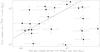 |
Fig. 11 Comparison of masses derived from the 875 μm dust continuum as well as via the C18O(2–1) line width under the assumption of virial equilibrium at the same spatial resolution of 27.5′′. We draw 25% error-bars although the real errors may be even larger as discussed in the main text. The solid line marks the 1:1 relation. The numbers in the bottom-right part correspond to the clumps discussed in the main text and marked in Fig. 4. |
4. Discussion
4.1. Different evolutionary stages and kinematic properties
As already mentioned in the introduction, the spatial offset between near-infrared clusters and UCHii regions toward the northern G10.3-0.1 and the southern G10.2-0.3 complex are indicative of several episodes of high-mass star formation within each of the subregions. Furthermore, as outlined in Sect. 3.1.1 and Fig. 3, within the G10.3-0.1 region, we not only have the infrared cluster and the UCHii region, but we also find at least one high-mass gas clump G10.3W2 without any cm or midinfrared emission indicative of star formation. Hence this clump may still be in a starless phase prior to active star formation. Therefore, from an evolutionary point of view, the northern G10.3-0.1 complex hosts several high-mass star-forming gas and dust clumps – all potentially capable of forming high-mass clusters – in at least three different evolutionary stages: a more evolved infrared cluster where the main sequence stars have already emerged, high-mass protostellar objects with and without embedded UCHii regions that may still be in an ongoing accretion phase, and high-mass starless clump candidates (see Table 1 for their parameters). Although there is no robust proof that the infrared cluster actually triggered the star formation processes in the neighboring clumps, the spatial structure with the infrared cluster almost at the geometrical center of G10.3-0.1, then the high-mass protostellar objects following in the surrounding, and the high-mass starless clump candidates at the edge of the region, indicates that triggered star formation may be a possible cause for the different evolutionary stages in this region.
Toward the southern G10.2-0.3 complex we also identify an infrared cluster and several high-mass protostellar objects, but there we do not as unambiguously find regions classifying as high-mass starless clump candidates. For a broader discussion of evolutionary sequences in high-mass star formation, we refer to the reviews by Beuther et al. (2007) and Zinnecker & Yorke (2007).
In addition to the evolutionary differences within each of the two main regions in W31, the kinematic analysis in Sect. 3.3 is also indicative of evolutionary differences between the two complexes in general. The virial mass as presented in Sect. 3.3 is directly proportional to the observed line width (Eq. (1)). In the simple virial equilibrium picture, having a ratio Mvir/Mpeak ~ 1 would imply that the clumps could be stable against collapse. However, except for a few notable sources like G10.3W2 (Fig. 3 and clump 6 in Fig. 4, see also Table 2 and Fig. 11) which are candidates for starless clumps, most other regions in this complex show various signs of star formation. Therefore, they are unlikely to be in virial equilibrium. It is rather the opposite, the feedback from ongoing star formation (e.g., outflows or radiation) significantly broadens the observed line width and the virial assumption cannot be properly applied under such circumstances.
While we do not know whether the clumps with high Mvir/Mpeak ratios are still bound or already expanding again from the inner energy sources, the fact that we see ongoing star formation indicates that they are still at least partly bound. Large virial parameters are also consistent with pressure-confined clumps as discussed by Bertoldi & McKee (1992) and more recently by Lada et al. (2008), Dobbs et al. (2011) and Kainulainen et al. (2011). High virial mass ratios have also been found by Simon et al. (2001) for four molecular clouds studied via the Galactic Ring Survey (GRS, Jackson et al. 2006). It is interesting to note that the three less evolved clouds of their sample have on average even higher virial mass ratios than their most luminous source, the galactic mini-starburst W49. The peak of their ratio between virial mass and LTE mass (derived via LTE calculations for the 13CO(1–0) emission) for W49 is around 2, whereas we find an average of Mvir/Mpeak for W31 of ~ 1.1. Hence, similar to W49 studied by Simon et al. (2001), the clumps in W31 are in the regime of being bound.
Maybe more surprising is that all high-mass clumps associated with G10.3-0.1 have Mvir/Mpeak ratios below 1. While this could be expected for the starless clump candidate G10.3W2 if it were in an unstable state just at the verge of collapse and had no additional turbulent support, it is less expected for the other active star-forming clumps where multiple additional line width broadening mechanisms should be at work, e.g., outflows and/or radiation. Nevertheless, low Mvir/Mpeak ratios clearly imply a comparatively small turbulent line width with respect to most of the clumps associated with the southern region G10.2-0.3. Furthermore, magnetic fields may be more important in these supposedly younger clumps acting as additional source of stability, also implying low Mvir/Mpeak ratios.
While the overall characteristics of the two complexes G10.2-0.3 and G10.3-0.1 appear similar – both have similar luminosities (see Sect. 1), strong submm and midinfrared emission as well as an associated near-infrared cluster – there is an apparent evolutionary difference between the two. In addition to the above discussed different Mvir/Mpeak ratios between G10.2-0.3 and G10.3-0.1, the class 0/I and class II sources around the southern G10.2-0.3 region appear considerably more widely distributed than those around the northern region G10.3-0.1 (see Sect. 3.1.1). Furthermore, it is also interesting to note that only G10.3-0.1 exhibits several sites of Class ii CH3OH masers whereas none is found toward G10.2-0.3 (Walsh et al. 1998). Since these CH3OH masers are also usually found toward younger regions (e.g., Fish 2007), the presence of them toward only the northern region G10.3-0.1 combined with additional differences discussed above strongly suggests that the northern G10.3-0.1 complex on average should be younger than the southern G10.2-0.3 region. The latter then had more time already to stir up the gas of the environment and thus increase the observed line width.
On top of all these evolutionary effects, we also find a closer association of the IRAC-identified younger class 0/I sources with the central high-mass gas clumps while the more evolved class II sources appear more broadly distributed over the whole field (Fig. 1).
4.2. The shape of the clump mass function
The power-law index α ~ 1.5 ± 0.3 of the clump mass function discussed in Fig. 5 (ΔN/ΔM ∝ M − α) is consistent with the clump mass function derived for molecular clouds by molecular line CO observations (α ~ 1.6, e.g., Stutzki & Guesten 1990; Blitz 1993; Kramer et al. 1998; Simon et al. 2001), but it is considerably flatter than distributions derived for other star-forming regions from dust continuum observations or extinction mapping, which resemble more the Salpeter slope (α ~ 2.35, e.g., Motte et al. 1998; Beltrán et al. 2006; Reid & Wilson 2006; Alves et al. 2007). In the past, the differences in power-law mass distributions derived from the different tracers (CO versus dust emission/extinction) was often attributed to the different density regimes they are tracing: the CO observations are more sensitive to the diffuse and transient gas whereas the dust emission/extinction rather traces the denser, gravitationally or pressure-bound cores. In this picture, the different power-law distributions would reflect a structural change of the cloud/clump properties from transient to bound structures.
However, this picture does not hold for our data of the W31 complex since we know that the region is actively star-forming and not a transient structure. Since cluster mass functions are also flatter than stellar mass functions (power-law distributions of 2.0, e.g., Bik et al. 2003; or de Grijs et al. 2003, versus 2.35 of the Salpeter slope, respectively), one possibility to explain the discrepancies is that we are tracing high-mass cluster-forming regions at far distances like W31 whereas the observations by Motte et al. (1998) or Alves et al. (2007) dissect low-mass regions like ρ Ophiuchus or the Pipe at distances closer ≤ 150 pc. Unfortunately, this explanation is not consistent with all observations since the mass distributions derived by Beltrán et al. (2006) or Reid & Wilson (2006) are also targeting high-mass star-forming regions at distances of several kpc.
Another possibility for a flatter clump mass function with respect to the IMF could be that the star formation efficiency (SFE) varies with clump mass. Higher mass gas clumps may exhibit on average a lower SFE that would steepen the slope from the clump mass function to the IMF. Similar results were recently inferred by Parmentier (2011). In a similar direction, it is worth noting that Simon et al. (2001) also inferred for their most luminous mini-starburst W49 the flattest clump mass function with a power-law index of 1.56, in very close agreement with our result for the high-luminosity region W31. Therefore, there are several indications that the most luminous regions could also exhibit the flattest clump mass functions.
One potentially more technical explanation for the relatively flat clump mass function we derive for W31 could be that our used uniform temperature of 50 K more severely affects α than we anticipated. Higher temperatures decrease the mass estimates of a clump whereas lower temperatures raise the mass estimates. In this picture, it could well be that the higher mass clumps closer to the centers of the region have higher temperatures whereas lower mass clumps may still be colder. This effect would steepen the mass function. Although with the current data we cannot properly quantify this effect, it is unlikely that the mass function would steepen to a Salpeter slope.
Therefore, we suggest that the observed flat mass function reflects that the resulting cluster mass functions are also flatter than the stellar initial mass function, and furthermore that the SFE may vary with clump mass.
5. Conclusions
The most luminous and high-mass star formation appears to take place in a highly structured and non-uniform fashion. The multiwavelength continuum and spectral line analysis of the different subregions within the very luminous W31 regions reveals evolutionary differences on large scales between the two subcomplexes G10.2-0.3 and G10.3-0.1, but also within each of these regions on much smaller scales. While many clumps have virial mass ratios close to unity, we also find low-turbulence, potentially still starless high-mass gas clumps that can reside in almost the direct vicinity of ongoing and already finished high-mass cluster-forming regions. The dense active gas clumps appear to be surrounded by a halo-like distribution of already more evolved class 0/1 and class II sources. We find a tight correlation between the warm dust tracing 24 μm emission and the ionized gas tracing cm emission, implying that warm dust at temperatures around 1000 K can spatially coexist with ionized gas in the 104 K regime. Furthermore, our data indicate that the clump mass function of W31 is considerably flatter (power-law index α ~ 1.5 ± 0.3) than the initial mass function, but it is consistent with the mass functions derived for other molecular clouds. Since these gas clumps trace cluster scales, this is consistent with the flatter cluster mass function compared to the stellar mass function. The analysis tentatively suggests that the star formation efficiency may decrease with increasing clump mass.
Online material
Clump parameters for original data.
Clump parameters for 27.5′′ resolution.
References
- Allen, L. E., Calvet, N., D’Alessio, P., et al. 2004, ApJS, 154, 363 [NASA ADS] [CrossRef] [Google Scholar]
- Alves, J., Lombardi, M., & Lada, C. J. 2007, A&A, 462, L17 [NASA ADS] [CrossRef] [EDP Sciences] [Google Scholar]
- Beltrán, M. T., Brand, J., Cesaroni, R., et al. 2006, A&A, 447, 221 [NASA ADS] [CrossRef] [EDP Sciences] [MathSciNet] [Google Scholar]
- Bertoldi, F., & McKee, C. F. 1992, ApJ, 395, 140 [NASA ADS] [CrossRef] [Google Scholar]
- Beuther, H., Schilke, P., Menten, K. M., et al. 2002, ApJ, 566, 945 [NASA ADS] [CrossRef] [Google Scholar]
- Beuther, H., Schilke, P., Menten, K. M., et al. 2005, ApJ, 633, 535 [NASA ADS] [CrossRef] [Google Scholar]
- Beuther, H., Churchwell, E. B., McKee, C. F., & Tan, J. C. 2007, in Protostars and Planets V, ed. B. Reipurth, D. Jewitt, & K. Keil, 165 [Google Scholar]
- Bik, A. 2004, Ph.D. Thesis [Google Scholar]
- Bik, A., Lamers, H. J. G. L. M., Bastian, N., Panagia, N., & Romaniello, M. 2003, A&A, 397, 473 [NASA ADS] [CrossRef] [EDP Sciences] [Google Scholar]
- Bik, A., Kaper, L., Hanson, M. M., & Smits, M. 2005, A&A, 440, 121 [NASA ADS] [CrossRef] [EDP Sciences] [Google Scholar]
- Blitz, L. 1993, in Protostars and Planets III, 125 [Google Scholar]
- Blum, R. D., Damineli, A., & Conti, P. S. 2001, AJ, 121, 3149 [NASA ADS] [CrossRef] [Google Scholar]
- Bonnell, I. A., Larson, R. B., & Zinnecker, H. 2007, in Protostars and Planets V, ed. B. Reipurth, D. Jewitt, & K. Keil, 149 [Google Scholar]
- Carey, S. J., Noriega-Crespo, A., Mizuno, D. R., et al. 2009, PASP, 121, 76 [NASA ADS] [CrossRef] [Google Scholar]
- Cesaroni, R., Churchwell, E., Hofner, P., Walmsley, C. M., & Kurtz, S. 1994, A&A, 288, 903 [NASA ADS] [Google Scholar]
- Churchwell, E., Babler, B. L., Meade, M. R., et al. 2009, PASP, 121, 213 [NASA ADS] [CrossRef] [Google Scholar]
- Corbel, S., Wallyn, P., Dame, T. M., et al. 1997, ApJ, 478, 624 [NASA ADS] [CrossRef] [Google Scholar]
- de Grijs, R., Anders, P., Bastian, N., et al. 2003, MNRAS, 343, 1285 [NASA ADS] [CrossRef] [Google Scholar]
- Dobbs, C. L., Burkert, A., & Pringle, J. E. 2011, MNRAS, 413, 2935 [NASA ADS] [CrossRef] [Google Scholar]
- Downes, D., Wilson, T. L., Bieging, J., & Wink, J. 1980, A&AS, 40, 379 [NASA ADS] [Google Scholar]
- Draine, B. T. 2003, ARA&A, 41, 241 [NASA ADS] [CrossRef] [Google Scholar]
- Draine, B. T., Dale, D. A., Bendo, G., et al. 2007, ApJ, 663, 866 [NASA ADS] [CrossRef] [Google Scholar]
- Everett, J. E., & Churchwell, E. 2010, ApJ, 713, 592 [NASA ADS] [CrossRef] [Google Scholar]
- Fish, V. L. 2007, in IAU Symp. 242, ed. J. M. Chapman, & W. A. Baan, 71 [Google Scholar]
- Fontani, F., Beltrán, M. T., Brand, J., et al. 2005, A&A, 432, 921 [NASA ADS] [CrossRef] [EDP Sciences] [Google Scholar]
- Ghosh, S. K., Iyengar, K. V. K., Rengarajan, T. N., et al. 1989, ApJ, 347, 338 [NASA ADS] [CrossRef] [Google Scholar]
- Güsten, R., Nyman, L. Å., Schilke, P., et al. 2006, A&A, 454, L13 [NASA ADS] [CrossRef] [EDP Sciences] [Google Scholar]
- Helfand, D. J., Becker, R. H., White, R. L., Fallon, A., & Tuttle, S. 2006, AJ, 131, 2525 [NASA ADS] [CrossRef] [Google Scholar]
- Hildebrand, R. H. 1983, QJRAS, 24, 267 [NASA ADS] [Google Scholar]
- Homeier, N. L., & Alves, J. 2005, A&A, 430, 481 [NASA ADS] [CrossRef] [EDP Sciences] [Google Scholar]
- Jackson, J. M., Rathborne, J. M., Shah, R. Y., et al. 2006, ApJS, 163, 145 [NASA ADS] [CrossRef] [Google Scholar]
- Jenkins, E. B. 2004, in Origin and Evolution of the Elements, ed. A. McWilliam, & M. Rauch, 336 [Google Scholar]
- Johnston, K. G., Shepherd, D. S., Aguirre, J. E., et al. 2009, ApJ, 707, 283 [NASA ADS] [CrossRef] [Google Scholar]
- Kainulainen, J., Beuther, H., Banerjee, R., Federrath, C. & Henning, T. 2011, A&A, 530, A64 [NASA ADS] [CrossRef] [EDP Sciences] [Google Scholar]
- Keto, E. 2002, ApJ, 568, 754 [NASA ADS] [CrossRef] [Google Scholar]
- Kim, K.-T., & Koo, B.-C. 2002, ApJ, 575, 327 [NASA ADS] [CrossRef] [Google Scholar]
- Klein, B., Philipp, S. D., Krämer, I., et al. 2006, A&A, 454, L29 [NASA ADS] [CrossRef] [EDP Sciences] [Google Scholar]
- Kramer, C., Stutzki, J., Rohrig, R., & Corneliussen, U. 1998, A&A, 329, 249 [NASA ADS] [Google Scholar]
- Kroupa, P. 2001, MNRAS, 322, 231 [NASA ADS] [CrossRef] [Google Scholar]
- Krumholz, M. R., & Bonnell, I. A. 2007 [arXiv:0712.0828] [Google Scholar]
- Krumholz, M. R., & McKee, C. F. 2008, Nature, 451, 1082 [NASA ADS] [CrossRef] [PubMed] [Google Scholar]
- Lada, C. J., Muench, A. A., Rathborne, J., Alves, J. F., & Lombardi, M. 2008, ApJ, 672, 410 [NASA ADS] [CrossRef] [Google Scholar]
- MacLaren, I., Richardson, K. M., & Wolfendale, A. W. 1988, ApJ, 333, 821 [NASA ADS] [CrossRef] [Google Scholar]
- McKee, C. F., & Ostriker, E. C. 2007, ARA&A, 45, 565 [NASA ADS] [CrossRef] [Google Scholar]
- Megeath, S. T., Allen, L. E., Gutermuth, R. A., et al. 2004, ApJS, 154, 367 [NASA ADS] [CrossRef] [Google Scholar]
- Molinari, S., Brand, J., Cesaroni, R., & Palla, F. 1996, A&A, 308, 573 [NASA ADS] [Google Scholar]
- Motte, F., Andre, P., & Neri, R. 1998, A&A, 336, 150 [NASA ADS] [Google Scholar]
- Mueller, K. E., Shirley, Y. L., Evans, N. J., & Jacobson, H. R. 2002, ApJS, 143, 469 [NASA ADS] [CrossRef] [Google Scholar]
- Parmentier, G. 2011, MNRAS, 413, 1899 [NASA ADS] [CrossRef] [Google Scholar]
- Plume, R., Jaffe, D. T., Evans, N. J., Martin-Pintado, J., & Gomez-Gonzalez, J. 1997, ApJ, 476, 730 [NASA ADS] [CrossRef] [Google Scholar]
- Qiu, K., Zhang, Q., Megeath, S. T., et al. 2008, ApJ, 685, 1005 [NASA ADS] [CrossRef] [Google Scholar]
- Reid, M. A., & Wilson, C. D. 2006, ApJ, 650, 970 [NASA ADS] [CrossRef] [Google Scholar]
- Rodón, J. A., Beuther, H., & Schilke, P. 2011, A&A, submitted [Google Scholar]
- Rohlfs, K., & Wilson, T. L. 2006, Tools of radio astronomy, 4th rev. and enl., ed. K. Rohlfs, & T. L. Wilson (Berlin: Springer) [Google Scholar]
- Sanders, D. B., Clemens, D. P., Scoville, N. Z., & Solomon, P. M. 1986, ApJS, 60, 1 [NASA ADS] [CrossRef] [Google Scholar]
- Schuller, F., Menten, K. M., Contreras, Y., et al. 2009, A&A, 504, 415 [NASA ADS] [CrossRef] [EDP Sciences] [Google Scholar]
- Simon, R., Jackson, J. M., Clemens, D. P., Bania, T. M., & Heyer, M. H. 2001, ApJ, 551, 747 [NASA ADS] [CrossRef] [Google Scholar]
- Sridharan, T. K., Beuther, H., Schilke, P., Menten, K. M., & Wyrowski, F. 2002, ApJ, 566, 931 [NASA ADS] [CrossRef] [Google Scholar]
- Stutzki, J., & Guesten, R. 1990, ApJ, 356, 513 [NASA ADS] [CrossRef] [Google Scholar]
- Thompson, M. A., Hatchell, J., Walsh, A. J., MacDonald, G. H., & Millar, T. J. 2006, A&A, 453, 1003 [NASA ADS] [CrossRef] [EDP Sciences] [Google Scholar]
- Vassilev, V., Meledin, D., Lapkin, I., et al. 2008, A&A, 490, 1157 [NASA ADS] [CrossRef] [EDP Sciences] [Google Scholar]
- Vasyunina, T., Linz, H., Henning, T., et al. 2009, A&A, 499, 149 [NASA ADS] [CrossRef] [EDP Sciences] [Google Scholar]
- Walsh, A. J., Burton, M. G., Hyland, A. R., & Robinson, G. 1998, MNRAS, 301, 640 [NASA ADS] [CrossRef] [Google Scholar]
- Walsh, A. J., Thorwirth, S., Beuther, H., & Burton, M. G. 2010, MNRAS, 404, 1396 [NASA ADS] [Google Scholar]
- Williams, J. P., de Geus, E. J., & Blitz, L. 1994, ApJ, 428, 693 [NASA ADS] [CrossRef] [Google Scholar]
- Wilson, T. L. 1974, A&A, 31, 832 [Google Scholar]
- Wood, D. O. S., & Churchwell, E. 1989, ApJS, 69, 831 [NASA ADS] [CrossRef] [Google Scholar]
- Woodward, C. E., Helfer, H. L., & Pipher, J. L. 1984, MNRAS, 209, 209 [NASA ADS] [Google Scholar]
- Zhang, Y., Huang, Y., Sun, J., & Lu, D. 2005, Chinese Astron. Astrophys., 29, 9 [NASA ADS] [CrossRef] [Google Scholar]
- Zinnecker, H., & Yorke, H. W. 2007, ARA&A, 45, 481 [NASA ADS] [CrossRef] [Google Scholar]
All Tables
All Figures
|
Fig. 1 Continuum images of the W31 region. The shown wavelengths are marked in each panel. The 875 μm data are contoured in 3σ steps from 3 to 12σ and continue in 15σ steps from 15σ onwards (1σ ≈ 70 mJy beam-1). The 21 cm image is contoured in 3σ steps from 3 to 12σ (1σ ≈ 5 mJy beam-1), continuing in 0.24 Jy beam-1 steps from 0.12 to 0.84 beam-1, and then go on in 0.48 beam-1 steps. The 24 μm map is saturated toward the peak positions. In the top-left panel the 3-pointed stars mark the position of an O-star by (Bik et al. 2005) and the approximate center of the southern infrared-cluster discussed by Blum et al. (2001). The two white 5-pointed stars show the positions of UCHii regions (Wood & Churchwell 1989). The ellipse marks the emission that velocity-wise is associated with cloud complexes outside our field of view (Sect. 3.2). A scalebar is shown in the top-left panel. The 875 μm and 21 cm beam sizes are shown in the top-right corners of the top-left and bottom-left panels, respectively. In the bottom-left panel, the triangles and stars show IRAC-identified protostellar class 0/I (the two classes are combined) and class II candidates, respectively, following Allen et al. (2004); Megeath et al. (2004); Qiu et al. (2008). |
| In the text | |
|
Fig. 2 Correlation between 24 μm fluxes and 21 cm fluxes for the W31 complex. Only pixels with 24 μm flux above 120 MJy sr-1 (corresponding to the approximate outskirts of the Hii regions) and 21 cm emission above the 3σ level of ~ 0.01Jy beam-1 are plotted. Furthermore, only correlations on scales of the beam size of the 21 cm observation were used (2-pixel steps corresponding to 29′′). |
| In the text | |
|
Fig. 3 Zoom into the G10.3 complex. In all 4 panels the solid contours present the 875 μm continuum contours (start at 3σ and continue in 9σ steps, 1σ ≈ 70 mJy beam-1) whereas the grey-scale shows other wavelength data as outlined over each panel. The dashed 21 cm contours in the right panel go from 15 to 60 mJy beam-1 in 15 mJy beam-1 steps, and from 120 to 840 mJy beam-1 in 240 mJy beam-1 steps. The K-band data are taken from Bik (2004). The white central part of the 24 μm image is saturated. The triangles in the left panel mark the Class ii CH3OH maser positions from Walsh et al. (1998). The white star in the right panel marks the position of an UCHii region (Wood & Churchwell 1989), and the additional labels there name sources discussed in the main text. |
| In the text | |
|
Fig. 4 The color-scales show the clump structure and boundaries derived with the automized clumpfind procedure on the original (left) and smoothed (right) 875 μm continuum observations. The contours show the original 875 μm observations with the same contour levels as in Fig. 1. The wedge reflects the clump numbers as in Tables 1 and 2. A few discussed clumps are labeled in the right panel (see also Fig. 11). |
| In the text | |
|
Fig. 5 Example clump mass function for the W31 complex for one bin size (here logarithmic bins with 10k ∗ 0.1 < M < 10(k + 1) ∗ 0.1 with k an integer, 36 different bin sizes have been used to overcome fitting artifacts). Only clumps with masses > 1000 M⊙ were used for the fit. |
| In the text | |
|
Fig. 6 13CO(2–1) and C18O(2–1) (multiplied by a factor 2) spectra averaged over the entire W31 region. The marked velocities show the different velocity regimes used for the 13CO (upper) and C18O (lower) moment maps. |
| In the text | |
|
Fig. 7 The grey-scale shows different 13CO(2–1) integrated intensity images where the integration regimes are shown in the top of each panel. Contour levels go from 20 to 80% in 20% levels of the respective peak intensities. The dotted contours outline the 875 μm emission at a 3σ level from Fig. 1. |
| In the text | |
|
Fig. 8 The grey-scale shows C18O(2–1) moment maps: 0th moment or integrated intensity on the left, 1st moment or intensity-weighted velocity in the middle and 2nd moment or intensity-weighted linewidth to the right. The black contours in the left panel show the integrated C18O(2–1) data and go from 20 to 80% in 20% steps. The dotted contours outline the 875 μm emission at a 3σ level from Fig. 1, and the red contours show additionally the high-intensity 875 μm emission in 15σ steps from 15σ onwards (1σ ≈ 70 mJy beam-1). In the right panel, the 3-pointed stars in the north and south mark the position of an O-star by Bik et al. (2005) and the center of the southern cluster discussed by Blum et al. (2001). The 5-pointed stars mark the two UCHii regions (Wood & Churchwell 1989). |
| In the text | |
|
Fig. 9 The grey-scale shows different 13CO(2–1) moment maps: 0th moment or integrated intensity on the left, 1st moment or intensity-weighted velocity in the middle and 2nd moment or intensity-weighted linewidth to the right. The black contours in the left panel show the integrated intensity 13CO(2–1) data from 20 to 80% in 20% steps. The dotted contours outline the 875 μm emission at a 3σ level from Fig. 1, and the red contours show additionally the high-intensity 875 μm emission in 15σ steps from 15σ onwards (1σ ≈ 70 mJy beam-1). In the right panel, the 3-pointed stars in the north and south mark the position of an O-star as reported by Bik et al. (2005) and the center of the southern cluster discussed by Blum et al. (2001). The 5-pointed stars mark the two UCHii regions (Wood & Churchwell 1989). |
| In the text | |
|
Fig. 10 Comparison of H2 column densities derived from the 875 μm dust continuum and C18O(2–1) at the same spatial resolution of 27.5′′. We draw 25% error-bars although the real errors may be even larger as discussed in the main text. The solid line marks the 1:1 relation. |
| In the text | |
|
Fig. 11 Comparison of masses derived from the 875 μm dust continuum as well as via the C18O(2–1) line width under the assumption of virial equilibrium at the same spatial resolution of 27.5′′. We draw 25% error-bars although the real errors may be even larger as discussed in the main text. The solid line marks the 1:1 relation. The numbers in the bottom-right part correspond to the clumps discussed in the main text and marked in Fig. 4. |
| In the text | |
Current usage metrics show cumulative count of Article Views (full-text article views including HTML views, PDF and ePub downloads, according to the available data) and Abstracts Views on Vision4Press platform.
Data correspond to usage on the plateform after 2015. The current usage metrics is available 48-96 hours after online publication and is updated daily on week days.
Initial download of the metrics may take a while.