| Issue |
A&A
Volume 525, January 2011
|
|
|---|---|---|
| Article Number | A125 | |
| Number of page(s) | 14 | |
| Section | Extragalactic astronomy | |
| DOI | https://doi.org/10.1051/0004-6361/201015540 | |
| Published online | 07 December 2010 | |
Comparison of the VIMOS-VLT Deep Survey with the Munich semi-analytical model
I. Magnitude counts, redshift distribution, colour bimodality, and galaxy clustering⋆
1
INAF – Osservatorio Astronomico di Brera,
via Bianchi 46, 23807
Merate,
Italy
e-mail: This email address is being protected from spambots. You need JavaScript enabled to view it.
2
INAF – Istituto di Astrofisica Spaziale e Fisica Cosmica di
Milano, via Bassini
15, 20133
Milano,
Italy
3
Max Planck Institut für Extraterrestrische Physik,
Giessenbachstrasse 1,
85748
Garching bei München,
Germany
4
Universitätssternwarte München, Scheinerstrasse 1, 81679
München,
Germany
5
INAF – Osservatorio Astronomico di Trieste,
via Tiepolo 11, 34131
Trieste,
Italy
6
Centre de Recherche Astrophysique de Lyon, UMR 5574, Université
Claude Bernard Lyon-École Normale Supérieure de Lyon-CNRS,
69230
Saint-Genis Laval,
France
7
Laboratoire d’Astrophysique de Marseille, UMR 6110,
CNRS-Université de Provence, 38 rue
Frédéric Joliot-Curie, 13388
Marseille,
France
8
Institut d’Astrophysique de Paris, UMR 7095, Université Pierre et
Marie Curie, 98bis Bd.
Arago, 75014
Paris,
France
9
The Andrzej Soltan Institute for Nuclear Studies,
ul. Hoza 69, 00-681
Warszawa,
Poland
10
Astronomical Observatory of the Jagiellonian
University, ul Orla 171,
30-244, Kraków,
Poland
11
INAF – Osservatorio Astronomico di Torino,
strada Osservatorio 20,
10025
Pino Torinese,
Italy
12
IRA-INAF, via
Gobetti 101, 40129
Bologna,
Italy
13
Canada France Hawaii Telescope corporation,
Mamalahoa Hwy, Kamuela, HI-96743, USA
14
INAF – Osservatorio Astronomico di Bologna,
via Ranzani 1, 40127
Bologna,
Italy
15
Laboratoire d’Astrophysique de Toulouse-Tarbes, UMR 5572,
CNRS-Université de Toulouse, 14 Av.
E. Belin, 31400
Toulouse,
France
16
Department of Earth Sciences, National Taiwan Normal
University, 88 Tingzhou Road, Sec.
4, Taipei
11677, Taiwan, PR China
17
Departamento de Ciencias Fisicas, Facultad de Ingenieria,
Universidad Andres Bello, Santiago, Chile
18
Centre de Physique Théorique, UMR 6207, CNRS-Université de
Provence, 13288
Marseille,
France
19
ISDC, Geneva Observatory, University of Geneva,
Ch. d’Ècogia 16,
1290
Versoix,
Switzerland
Received: 6 August 2010
Accepted: 2 October 2010
Abstract
Aims. This paper presents a detailed comparison between high-redshift observations from the VIMOS-VLT Deep Survey (VVDS) and predictions from the Munich semi-analytical model of galaxy formation. In particular, we focus this analysis on the magnitude, redshift, and colour distributions of galaxies, as well as their clustering properties.
Methods. We constructed 100 quasi-independent mock catalogues, using the output of the semi-analytical model presented in De Lucia & Blaizot (2007, MNRAS, 375, 2). We then applied the same observational selection function of the VVDS-Deep survey, so as to carry out a fair comparison between models and observations.
Results. We find that the semi-analytical model reproduces well the magnitude counts in the optical bands. It tends, however, to overpredict the abundance of faint red galaxies, in particular in the i′ and z′ bands. Model galaxies exhibit a colour bimodality that is only in qualitative agreement with the data. In particular, we find that the model tends to overpredict the number of red galaxies at low redshift and of blue galaxies at all redshifts probed by VVDS-Deep observations, although a large fraction of the bluest observed galaxies is absent from the model. In addition, the model overpredicts by about 14 per cent the number of galaxies observed at 0.2 < z < 1 with IAB < 24. When comparing the galaxy clustering properties, we find that model galaxies are more strongly clustered than observed ones at all redshift from z = 0.2 to z = 2, with the difference being less significant above z ≃ 1. When splitting the samples into red and blue galaxies, we find that the observed clustering of blue galaxies is well reproduced by the model, while red model galaxies are much more clustered than observed ones, being principally responsible for the strong global clustering found in the model.
Conclusions. Our results show that the discrepancies between Munich semi-analytical model predictions and VVDS-Deep observations, particularly in the galaxy colour distribution and clustering, can be explained to a large extend by an overabundance of satellite galaxies, mostly located in the red peak of the colour bimodality predicted by the model.
Key words: cosmology: observations / large-scale structure of Universe / galaxies: evolution / galaxies: high-redshift / galaxies: statistics
Based on data obtained with the European Southern Observatory Very Large Telescope, Paranal, Chile, program 070.A-9007(A), and on data obtained at the Canada-France-Hawaii Telescope, operated by the CNRS of France, CNRC in Canada and the University of Hawaii. This work is based in part on data products produced at TERAPIX and the Canadian Astronomy Data Centre as part of the Canada-France-Hawaii Telescope Legacy Survey, a collaborative project of NRC and CNRS.
© ESO, 2010
1. Introduction
Most accurate cosmological probes tend to favour a flat ΛCDM cosmological model and strengthen the hierarchical growth of structure scenario (e.g. Riess et al. 1998; Spergel et al. 2003; Tegmark et al. 2004; Komatsu et al. 2009). In this picture, it is believed that the onset of galaxy formation arises inside dark matter haloes and that the cosmic history of galaxies follows the hierarchical evolution of haloes.
Despite the undeniable successes of the ΛCDM model to explain a broad variety of astrophysical observations, the description of stellar mass assembly and star formation activity in this framework and its confrontation to observations remain challenging (e.g. De Lucia 2009). The most recent deep galaxy spectroscopic surveys (e.g. Davis et al. 2003; Dickinson et al. 2003; Le Fèvre et al. 2005a; Lilly et al. 2007), that enabled the census of galaxy properties up to z ≃ 2, have confirmed that the so-called downsizing scenario (Gavazzi et al. 1996; Cowie et al. 1996), is a primary feature of galaxy formation. About half of the stellar mass in massive galaxies observed at the present time was already in place at z ≃ 1 (e.g. Bundy et al. 2005; Cimatti et al. 2006; Arnouts et al. 2007; Ilbert et al. 2010), while the number density of less massive galaxies continues to rise with cosmic time even for redshifts below unity. Most massive galaxies cease to efficiently produce new stars earlier than lower mass galaxies, which keep producing stars until very recent times (e.g. Tresse et al. 2007). This scenario is also supported by most recent observations of the VIMOS-VLT Deep Survey (VVDS, Le Fèvre et al. 2005a), one of the largest spectroscopic surveys of distant galaxies. In particular, the VVDS-Deep sample provides one with a description of the high-redshift Universe from z ≃ 0.2 to z ≃ 2, where the evolution of the galaxy luminosity function (Ilbert et al. 2005; Zucca et al. 2006), galaxy stellar mass function (Pozzetti et al. 2007), star formation rate (Tresse et al. 2007; Bardelli et al. 2009), colour bimodality (Franzetti et al. 2007), and galaxy clustering (Le Fèvre et al. 2005b) cannot be only explained by a simple scenario of hierarchical growth of baryons.
The complex physical processes involving baryons on galactic scales likely explain why the physics of stellar mass assembly and star formation is still puzzling in the ΛCDM model. Fortunately, large N-body simulations coupled with semi-analytical treatments of baryonic processes or fully hydrodynamical simulations have become sufficiently sophisticated to draw detailed and reliable predictions for galaxy properties (e.g. Weinberg et al. 2004; Springel et al. 2005; Kim et al. 2009b). Current semi-analytical models can be tuned to optimally reproduce some of the basic galaxy properties observed in the local Universe such as the galaxy luminosity function or the Tully-Fisher relation. Galaxy mock samples constructed from these models are widely used for a large variety of purposes. However, it is not yet demonstrated that numerical simulations together with semi-analytical model can successfully describe galaxy properties at high redshift and the physics driving the evolution of the various galaxy populations. There have been few detailed comparisons made between their predicted galaxy properties and a broad range of observational measurements at high redshift. Most comparisons were focused on single observations that has provided important clues, but still a limited perspective on the global galaxy evolution scenario.
Bower et al. (2006) compare the K-band luminosity function, galaxy stellar mass function, and cosmic star formation rate from the Durham model (Bower et al. 2006) with high-redshift observations. They find that their model match the observed mass and luminosity functions reasonably well up to z ≃ 1. Kitzbichler & White (2007) compare the magnitude counts in B,R,I,K bands, redshift distributions for K-band selected samples, B- and K-band luminosity functions, and galaxy stellar mass function from the Munich model (Croton et al. 2006; De Lucia & Blaizot 2007) with deep surveys measurements. They find that the agreement of the Munich model with high-redshift observations is slightly worse than that found for the Durham model. In particular, they find that the Munich model tends to systematically overestimate the abundance of relatively massive galaxies at high redshift. They note, however, a non-negligible dispersion between various observations.
The predicted galaxy clustering properties by semi-analytical models have been mainly compared with local observations (e.g. Springel et al. 2005; Li et al. 2006, 2007; Kim et al. 2009a). Similar conclusions are obtained when confronting models to 2dFGRS (Colless et al. 2001) and SDSS (York et al. 2000) measurements: semi-analytical models are able to reproduce the overall observed clustering properties, but fail to predict the measurements in details, e.g. the different clustering of red and blue galaxies (Springel et al. 2005). For the high-redshift Universe, only few data-model comparisons have been carried out (McCracken et al. 2007; Coil et al. 2008; Meneux et al. 2008, 2009). These studies highlight a number of discrepancies between model predictions and observations. In particular, Coil et al. (2008) show that red model galaxies are more strongly clustered than observed at z ≃ 1, particularly on small scales. Blue galaxies in the model show instead a lower clustering strength than observed, suggesting a significant deficit of blue satellite galaxies in the semi-analytical model of Croton et al. (2006). They interpret these discrepancies as due to an incorrect modelling of the colours of satellite galaxies at high redshift.
In this paper, we compare the basic galaxy properties observed in the VVDS-Deep spectroscopic sample at 0.2 < z < 2 to the outputs of the Munich model. This is the first of a series of papers that aim at a detailed comparison between model predictions and a complete set of galaxy properties and their evolution with cosmic time, derived from the VVDS-Deep observations. In this first paper, we focus on the magnitude counts, redshift distribution, colour bimodality, B-band and I-band luminosity distributions, and the global clustering measurements. The detailed dependence of galaxy clustering on luminosity and intrinsic colour is the subject of a forthcoming paper (Meneux et al. in prep., hereafter Paper II).
In Sect. 2 we summarise the basic characteristics of the VVDS-Deep sample and the Munich semi-analytical model. In Sect. 3 we compare the observed magnitude counts, redshift distribution, colour bimodality, B-band, and I-band luminosity distributions with model predictions. In Sect. 4 we present the galaxy clustering comparison and we discuss our results in Sect. 5. Throughout this paper we assume a flat ΛCDM cosmology with ΩM = 0.25, ΩΛ = 0.75 and H0 = 100 h km s-1 Mpc-1. All magnitudes are quoted in the AB system and for simplicity we denote the absolute magnitude Mx−5log (h) as Mx.
2. VVDS-Deep sample and Munich galaxy formation model
2.1. The VVDS-Deep spectroscopic sample
The VIMOS-VLT Deep Survey (VVDS, Le Fèvre et al. 2005a) is a deep spectroscopic survey of galaxies performed with the VIsible Multi-Object Spectrograph (VIMOS, Le Fèvre et al. 2003) at the European Southern Observatory’s Very Large Telescope (ESO–VLT). The deep part of the survey (VVDS-Deep) spans the apparent magnitude range 17.5 < IAB < 24 and contains about 8700 galaxies over an area of 0.49 deg2. In addition to VIMOS spectroscopy, the field has a multi-wavelength photometric coverage: B, V, R, I from the VIRMOS Deep Imaging Survey (VDIS, Le Fèvre et al. 2004), u ∗ , g′, r′, i′, z′ from the Canada France Hawaii Telescope Legacy Survey1 (CFHTLS-D1, Goranova et al. 2009; Coupon et al. 2009), and a partial coverage in J and K bands from VDIS (Iovino et al. 2005).
Unless otherwise stated, in this analysis we use only the galaxies with secure redshift, i.e. which have a redshift confidence level greater than 80% (flag 2 to 9, see Le Fèvre et al. 2005a). This provides us with a spectroscopic sample of 6582 galaxies. The accuracy of the redshift measurements is of σz = 9.2 × 10⁻⁴. The observational spectroscopic strategy allows us to reach an average spectroscopic sampling rate of 27% across the field. The observations, survey strategy, and basic properties of the VVDS-Deep sample are described in detail in Le Fèvre et al. (2005a). The VVDS-Deep spectroscopic catalogue is publicly available through the CENter for COSmology database (CENCOS) site2.
Absolute magnitudes for VVDS-Deep galaxies have been computed by Ilbert et al. (2005) and properly k-corrected using the spectral template that best fits the B, V, R, I photometry. The VVDS-Deep apparent and absolute magnitudes used in this study are not corrected for intrinsic dust attenuation.
2.2. The galaxy formation model
In this study, we take advantage of the semi-analytical model presented in De Lucia & Blaizot (2007), whose outputs are publicly available through the Millennium Simulation database site3. The model is implemented on the Millennium Run N-body simulation, a large dark matter N-body simulation which traces the hierarchical evolution of 21603 particles between z = 127 and z = 0 in a cubic volume of 5003 h-3 Mpc3. It assumes a ΛCDM cosmological model with (Ωm = Ωdm + Ωb, ΩΛ, Ωb, h, n, σ8) = (0.25, 0.75, 0.045, 0.73, 1, 0.9). The resolution of the N-body simulation, 8.6 × 10⁸ h-1 M⊙, coupled with the semi-analytical model allows one to resolve haloes containing galaxies with a luminosity of 0.1 L ∗ with a minimum of 100 particles. Haloes and sub-haloes are identified from the spatial distribution of dark matter particles using a standard friends-of-friends algorithm and the SUBFIND algorithm (Springel et al. 2001). All sub-haloes are then linked together to construct the halo merging trees which represent the basic input of the semi-analytical model. Details about the simulation and the merger tree construction can be found in Springel et al. (2005).
Galaxies are simulated on top of the dark matter simulation using the information contained in the halo merging trees. The semi-analytical model (SAM) used in this study includes ingredients and methodologies originally introduced by White & Frenk (1991) and later refined by Kauffmann & Haehnelt (2000), Springel et al. (2001), De Lucia et al. (2004), Croton et al. (2006), and De Lucia & Blaizot (2007). The model includes prescriptions for gas accretion and cooling, star formation, feedback, galaxy mergers, formation of super-massive black holes, and treatment of “radio mode” feedback from galaxies located at the centres of groups or clusters of galaxies (see Croton et al. 2006, for details). One important aspect in the modelling of galaxy properties at high redshift is dust extinction. This effect is particularly critical when modelling galaxy magnitudes (Kitzbichler & White 2007; Fontanot et al. 2009b). In this work we have used the dust extinction model of De Lucia & Blaizot (2007), where dust extinction is parametrised using a homogeneous interstellar medium component combined with a simple model for molecular clouds attenuation around newly formed stars. In the following, we will often refer to this model as the “Munich” model.
2.3. Mock samples construction
In order to compare the galaxy properties predicted by the model with VVDS-Deep observations, we generated mock samples that cover the same volume probed by the VVDS-Deep sample, as viewed by an observer at z = 0. These have been constructed using the MoMaF facility (Blaizot et al. 2005), which converts the output of a galaxy formation model into simulated catalogues of observations. In particular, the light-cone construction adopted in MoMaF avoids replication and finite-volume effects in constructing mock survey catalogues.
We built 100 quasi-independent mock samples of 0.49 deg2 providing the apparent magnitudes in the VDIS and CFHTLS filters for all galaxies. In computing magnitudes, we use the appropriate filter transmission curves of the VDIS and CFHTLS photometric bands. These mock samples are linked to the main SAM output, providing the full set of intrinsic galaxy properties that the model calculates, as for instance galaxy absolute magnitudes and host halo properties. The VVDS-Deep galaxy selection criterion, 17.5 < IAB < 24, has been applied to the mock samples. These mock samples mimic the expected VVDS-Deep sample with a spectroscopic sampling rate of 100% and a uniform sampling on the sky. Hereafter, we will refer to them as the “complete” mock samples: Cmocks.
From the Cmocks we constructed a second set of mock samples that include the detailed observational selection function and biases of the VVDS-Deep sample, and in particular, its complex angular sampling. These have been constructed using the following procedure:
-
Photometric
mask.
In the VDIS images, objects falling in bad photometric regions or in areas where the presence of bright stars saturates the CCD, have been removed from the photometric catalogue. Consequently, no objects inside these regions have been targeted for spectroscopy. In practice, these regions have been identified and coded into a photometric mask, that we applied to the mock samples. This reproduces in the simulated catalogues the various empty regions present in the angular distribution of objects in the VVDS-Deep (see Fig. 2 ).
-
Target sampling rate.
The SSPOC software ( Bottini et al. 2005) has been used to prepare VVDS-Deep observations, performing the design of the slit masks for the planned VIMOS pointings. This software, which accounts for the precise shape of the VIMOS field-of-view (4 quadrants delimited by an empty cross), enables one to optimise the slit positioning and to maximise the number of objects observed in spectroscopy from a given list of potential targets. Similarly, we applied SSPOC to the mock samples giving as input the list of VIMOS observed pointings in the VVDS-Deep. SSPOC requires the angular size of objects. Since this property is not attributed to mock galaxies by the model, we randomly assigned an apparent radius to mock galaxies, in a way to reproduce the observed distribution of apparent radii as a function of the selection magnitude in the VVDS-Deep. In the optimisation process, SSPOC tends to preferentially select objects with smaller apparent angular size. This introduces a mild bias against large galaxies, on average brighter, which we will refer to as the target sampling rate (TSR) in the following (Ilbert et al. 2005).
-
Spectroscopic success rate.
Galaxy redshifts in the VVDS-Deep sample have been determined from the observed spectra. In this process, a confidence class is given to each targeted object to quantify its type and the confidence level on the redshift determination (Le Fèvre et al. 2005a). In general, redshifts of galaxies with brighter apparent magnitudes, and in turn with higher signal-to-noise spectra, have a larger probability to be measured. The success in determining galaxy redshifts is thus a function of the apparent magnitude. This introduces a bias against faint objects which we will refer to as the spectroscopic sampling rate (SSR) in the following (Ilbert et al. 2005). To reproduce this selection bias in the mock samples, we randomly assigned a flag to each mock galaxy, in a way to match the dependence of the fraction of the different redshift confidence flags on the apparent magnitude in the VVDS-Deep. We kept in the mock samples the galaxies with flag 2 to 9, corresponding to objects with secure redshift in the VVDS-Deep (confidence level greater than 80%, Le Fèvre et al. 2005a). Figure 1 shows the fraction of galaxies with secure redshift measurements over the total number of spectroscopic targets in the VVDS-Deep, as a function of the apparent magnitude of selection. The solid curve in the same figure shows the mean measurement from the mock samples.
By applying this procedure to the Cmocks samples, we end up with a new set of mock samples having on average a mean sampling rate of 27% (identical to that of the VVDS-Deep), and that include the detailed selection function and observational biases of the VVDS-Deep spectroscopic sample. The angular distribution of galaxies in the mock sample 1 obtained following this procedure is shown as an example in Fig. 2 and compared to that of the VVDS-Deep secure redshift sample. In the following, we will refer to these mock samples as the “observed” mock samples: Omocks.
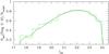 |
Fig. 1 Fraction of the number of galaxy with secure redshift (flag 2 to 9) over the total number of spectroscopic targets in the VVDS-Deep as a function of the I apparent magnitude (histogram). The solid curve is the average fraction over the Omocks samples. |
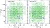 |
Fig. 2 Angular distribution of galaxies in the VVDS-Deep (left) and in the Omocks sample 1 (right). The galaxies are shown with the dots and the background coloured areas encode the surface density of objects. The solid contours encompass the regions discarded by the photometric mask. |
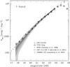 |
Fig. 3 Comparison of the magnitude counts in the VDIS I-band with SAM predictions and previously reported measurements by Postman et al. (1998) in the KPNO survey, Leauthaud et al. (2007) in the COSMOS-ACS field, and Metcalfe et al. (2001) in the Hubble Deep Field-North & South. The VVDS-Deep counts are shown with the empty squares and the error bars correspond to their associated Poisson errors. The solid curve and associated shaded areas are respectively the mean and the 1σ, 2σ, and 3σ field-to-field dispersions among Cmocks samples. |
3. Number counts
3.1. Magnitude counts
We compare the galaxy magnitude counts in the VDIS I-band (selection band) and in the CFHTLS u ∗ ,g′,r′,i′,z′ bands with those predicted by the SAM. In this comparison, we use all galaxies with VDIS photometry for I-band counts, while for u ∗ ,g′,r′,i′,z′ counts, we use all galaxies with CFHTLS-D1 photometry falling in the VDIS field. The effective areas probed are 1.19 deg2 and 0.89 deg2 respectively. We used Cmocks samples of same angular sizes. The VDIS and CFHTLS photometric catalogues reach limiting magnitudes (80% completeness for point-like sources) of 24.6, 26.2, 25.9, 25.4, 25.1, 24.6 respectively for I,u ∗ ,g′,r′,i′,z′ bands (see McCracken et al. 2003; Goranova et al. 2009). When computing the magnitude counts in the VVDS data, we carefully excluded stars using colour-colour diagrams following McCracken et al. (2003).
We first compare the I-band galaxy counts in the VDIS field with published measurements from large and deep photometric surveys. This comparison is shown in Fig. 3. We find a very good agreement between the VVDS and other published I-band counts in the literature (see also McCracken et al. 2003). When comparing to the SAM predictions, we find that the predicted I-band counts match very well the VVDS-Deep ones at I > 20. The model, however, slightly underpredicts the number of galaxies brighter than I ≃ 20. On average, the mock samples contain 10.3% less galaxies than observed at 17.5 < I < 24 in the VVDS-Deep. In Fig. 4 we compare the predicted magnitude counts in the CFHTLS bands with the observational measurements. Note that in this figure, the CFHTLS counts extend above 24 mag, while the SAM mock samples have been cut at I = 24 to match the VVDS-Deep selection function. We find that the observed and predicted counts are in very good agreement, except in the i′- and z′-bands where the SAM predicts more galaxies at the faintest magnitudes. While in the i′-band the counts are compatible within the 3σ field-to-field dispersion among the mock samples, the z′-band counts deviate from the VVDS-Deep at more than 3σ for magnitudes fainter than z′ = 22.
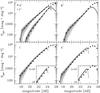 |
Fig. 4 Comparison of the magnitude counts in the CFHTLS u ∗ , g′, r′, i′, z′ optical bands with SAM predictions for 17.5 < I < 24 galaxies. The CFHTLS counts are shown with the squares and the error bars correspond to their Poisson errors. The curves and associated shaded areas are respectively the mean and the 1σ, 2σ, and 3σ field-to-field dispersions among the Cmocks samples. SAM predictions are for samples explicitly cut at I = 24, while CFHTLS counts extend above this limit. All galaxies with I < 17.5 have been removed from the counts. |
Similar small discrepancies between model predictions and observed magnitude counts were found by Kitzbichler & White (2007) who, however, used observational measurements based on smaller samples. In particular, they compared the counts in the B, R, I bands as observed over an area of 0.2 deg2 in the Hubble Deep Field North (HDF-N), and in K-band, in fields of area smaller than 0.1 deg2. They found a very good agreement between model predictions and observations in the B, R, I bands, with only a small underestimation of the predicted counts at I < 19.5. For K-band counts, the agreement they found was less good with the counts becoming discrepant at K > 21 by a factor of 2. These results are fully consistent with ours.
3.2. Redshift distribution
To provide a fair comparison of the VVDS-Deep redshift distribution with that predicted by the SAM, we first consider only the VVDS-Deep galaxies with secure redshifts (flag 2 to 9), which represent 75% of the full galaxy sample. The remaining 25% of the sample is made of galaxies with a redshift confidence level of about 50% (flag 1, 17%) and unclassified objects for which no redshift measurement has been possible (flag 0, 8%). Note that this latter class possibly includes stars. As redshifts are available only for about 27% of the galaxies with 17.5 < I < 24, we normalise the redshift distribution to the total number of galaxies in the parent photometric catalogue. The corresponding redshift distribution is shown in Fig. 5 with the solid thin histogram. This normalisation assumes that the spectroscopic sample is statistically representative of the parent photometric catalogue and that there are no biases introduced by the particular spectroscopic targeting strategy adopted. In reality, both these assumptions are incorrect.
 |
Fig. 5 Comparison of the VVDS-Deep with the SAM redshift distributions for 17.5 < IAB < 24 galaxies. The VVDS-Deep N(z), while including only flag 2 to 9 galaxies, is shown with the solid thin histogram. The thick histogram corresponds to the corrected N(z) in the VVDS-Deep when accounting for the observational biases of the survey (see text for details). The solid curve and associated shaded area are the mean and the 1σ field-to-field dispersion among the Omocks, while the dotted curve is the mean prediction of the Cmocks. |
In order to account for the observational biases and estimate their influence on the observed redshift distribution, we use the information of the survey target sampling rate (TSR) and spectroscopic sampling rate (SSR) available for each galaxy of the sample. These two functions have been originally defined to correct for the observational biases in the measurement of the galaxy luminosity function (Ilbert et al. 2005; Zucca et al. 2006). The SSR accounts for the fraction of objects without a reliable redshift determination (flag 0 and flag 1 galaxies) and corrects for the fact that the success rate of redshift measurements decreases at fainter apparent magnitudes. The TSR instead, corrects for the selection biases introduced by SSPOC software in the spectroscopic mask preparation (Bottini et al. 2005), e.g. its tendency to target objects with small apparent angular size. Within the Ultra-Deep part of the VVDS survey Le Fèvre et al. (in prep.), a small fraction of flag 0, flag 1, and flag 2 galaxies have been reobserved. These reobservations, representing 4% of the total number of objects in the spectroscopic catalogue, have permitted us to refine the measurement of the TSR and SSR functions, allowing us to better statistically account for the spectroscopic incompleteness. The VVDS-Ultra-Deep observations, as well as details on the calculation of the TSR and SSR are given in Le Fèvre et al. (in prep).
We correct the raw redshift counts, including flag 1 galaxies, by weighting each galaxy by w = (TSR × SSR)-1. The corrected redshift distribution is shown in Fig. 5 with the solid thick histogram. The solid curve and associated shaded area correspond to the predicted mean N(z) and the 1σ field-to-field dispersion among Omocks samples, which provides an estimate of the sample variance in the model. The predicted mean N(z) of the Cmocks samples is plotted with the dotted curve.
We first note that VVDS-Deep observational biases have little effect on the shape of the predicted redshift distribution in the mock samples: the mean N(z) obtained from Omocks is very similar to that of Cmocks. The SAM well reproduces the shape of the observed distribution between z ≃ 1 and z ≃ 1.8 while it shows an excess of about 14 per cent with respect to the observations at 0.2 < z < 1. Similar trends were found in Kitzbichler & White (2007) who noted that the predicted redshift distribution was higher than observed over the redshift range 0.5 < z < 1.5 for K < 21.8 galaxies. As we will discuss in the next section, this excess is related to an excess of red galaxies at z < 1 in the model. Furthermore, we find that the model does not account for the tail of the distribution at redshifts above z ≃ 2 and that extends to z ≃ 4 in the VVDS-Deep sample. In fact the SAM does not predict any galaxy at z > 3 with I < 24. The dip observed at 1.8 < z < 3 in the VVDS-Deep uncorrected N(z) is a purely observational effect usually referred as the “redshift desert”. It is due to the lack of spectral features in galaxy spectra observed within the wavelength window function of the spectrograph at these redshifts (Le Fèvre et al. 2005a). VVDS-Ultra-Deep reobservations, based on spectra measured on a larger wavelength range (VIMOS LR-Blue plus LR-Red grisms), allow us to correct for this observational effect and to repopulate the “redshift desert” at 1.8 < z < 3. Indeed, a large fraction of the reobserved galaxies falls in this part of the redshift distribution, and thus by properly weighting the original flag 1 to 9 galaxies we are able to statistically account for the missing fraction of objects at these redshifts (see Le Fèvre et al., in prep.).
Definition and properties of VVDS-Deep samples.
Definition and mean properties of the Munich semi-analytical model Cmocks samples.
3.3. Galaxy luminosity and intrinsic colour distributions
Galaxies are found to have a bimodal colour distribution and rest-frame colours are commonly used to differentiate red massive early-type from blue star-forming late-type galaxies. Here we define these two populations on the basis of the rest-frame B − I colour distribution. We made this particular choice because it corresponds to the optimal rest-frame colour that can be measured both in the VVDS-Deep and in the model (the rest-frame U-band is not available in the SAM). We considered six redshift intervals from z = 0.2 to z = 2.1, and compare the rest-frame B-band, I-band, and B − I distributions from the model with the observational measurements. The definition of the samples and their basic properties are given in Tables 1 and 2. The galaxy luminosity and rest-frame colour distributions (normalised to unity) in the VVDS-Deep and the SAM are presented in Figs. 6 and 7.
 |
Fig. 6 Comparison of the rest-frame B-band (right panels) and I-band (left panels) distributions in six magnitude-limited samples from z = 0.2 to z = 2.1. The histograms are VVDS-Deep measurements while the curves and associated shaded areas correspond to the mean and the 1σ field-to-field dispersion among the Omocks samples. The dashed curves are the mean distribution in the Omocks without including dust extinction in the model, while the dotted ones are the mean predictions of the Cmocks. |
 |
Fig. 7 Comparison of the rest-frame B − I distribution in six magnitude-limited samples from z = 0.2 to z = 2.1. In each panel, the histogram corresponds to the VVDS-Deep measurement while the curve and associated shaded area correspond to the mean and the 1σ field-to-field dispersion among the Omocks samples. The dashed curves are the mean distribution in the Omocks without including dust extinction in the model, while the dotted ones are the mean predictions of the Cmocks. |
The predicted rest-frame B-band distributions in the different redshift intervals are in good agreement with VVDS-Deep observations (the apparent discrepancy in the peak height in the last high-redshift interval is not statistically significant given the small number of galaxies involved). This indicates that the B-band luminosity function may be well reproduced in the SAM up to z ≃ 2 as also found by Kitzbichler & White (2007) at 0.2 < z < 1.2. Instead, we find that the rest-frame I-band distributions are systematically skewed towards bright magnitudes in the SAM. The effect is particularly important at z > 0.9 where the model tends to significantly overestimate the number of galaxies with −23 < MI < −21. A similar trend was found in Kitzbichler & White (2007) when confronting the K-band luminosity function, although the small observational samples they used did not allow them to reach firm conclusions.
When comparing the intrinsic colour distributions, we find that the rest-frame B − I colour distribution is clearly bimodal both in the VVDS-Deep and in the model, but the agreement is only qualitative. As shown in Fig. 7, the SAM does not reproduce quantitatively the observed intrinsic colour distributions: there are many fewer very blue galaxies (i.e. with B − I ≃ 0.3) and much more “green valley” galaxies (i.e. with B − I ≃ 1) in the model than in the observations, at all probed redshifts. In addition, the model predicts an excess of red galaxies at low redshift. It could be argued that part of the discrepancies between the SAM and observed colours could be related to uncertainties in the modelling of dust extinction (e.g. Kitzbichler & White 2007; Fontanot et al. 2009b). The dashed line in Fig. 7 shows the rest-frame B − I colour distribution in the SAM without including dust extinction in the model galaxies. In that case, when comparing to VVDS-Deep colour distributions, one finds that while in the highest-redshift intervals the predicted and observed colour distributions are quite similar, the lack of blue galaxies in the model is remarkable at z < 1.1. Franzetti et al. (2007) show that the fixed apparent magnitude selection of the VVDS-Deep sample can in principle introduce a mild bias in the intrinsic colours, partially displacing rest-frame U − V colours towards the blue at z > 1.2. However, they find that this effect is marginal and cannot be invoked to explain the discrepancies found in the SAM at all probed redshift. Intrinsically, the SAM may not form enough very blue galaxies.
Because of the discrepancies between the predicted and observed colour distributions, it is difficult and possibly meaningless to define “blue” and “red” galaxies using the same colour cut. We therefore opted to use a different colour cut for the SAM and the VVDS-Deep sample, with the aim of separating blue and red populations on the basis of the colour bimodality. In the VVDS-Deep we use a cut at (B − I)cut = 0.95. Zucca et al. (2006) show that galaxies selected above and below this value largely overlap with those classified as early- and late-type galaxies using a more refined method based on spectral energy distribution fitting. We adopt a larger value of (B − I)cut = 1.3 to separate red and blue populations in the SAM. We compare in Fig. 8 the total number and the fraction of red and blue galaxies at different redshifts.
We find a large difference in the number density of blue galaxies as predicted by the SAM and observed in the VVDS-Deep. While the trends with redshift are rather similar, the SAM predicts 50–80% more blue galaxies than observed over the whole redshift interval 0.2 < z < 1.6 in the VVDS-Deep. In the observations we find the presence of an already significant number of red galaxies at z ≃ 1.5. This number increases until z ≃ 0.8 and then slightly decreases with cosmic time. In contrast, the SAM predicts a monotonic increase with time of the number of red galaxies. Above z ≃ 0.8, the total number of red galaxies is smaller in the model than in the observations but the trend reverses at later epochs, where the total number of red VVDS-Deep galaxies starts to decline and that of red model galaxies continues to rise slowly. These same problems are evident when looking at the fractions of the two populations (bottom panel in Fig. 8). The SAM predicts a monotonic decrease (increase) of the fraction of blue (red) galaxies with time at variance with VVDS-Deep sample, in which this trend reverses at z < 0.8. Note that we discuss the variation with cosmic time of the number and fraction of red and blue galaxies in terms of apparent increase or decrease in a given apparent magnitude range, which does not necessarily imply real increase or decrease in number density at these redshifts.
At redshifts higher than z ≃ 0.8, the number of red galaxies is slightly lower in the SAM with respect to observations, while blue galaxies appear to be significantly more abundant at all cosmic epochs. This indicates that the overabundance of galaxies previously seen in the redshift distribution below z ≃ 0.8−1 in the SAM (Fig. 5), is due to the presence of a larger number of both blue (true at all redshifts for this colour) and red galaxies.
The difference in the variation with cosmic time of the fraction of red and blue galaxies and of the shape of the rest-frame B − I colour distribution in the SAM, suggests that these populations may have different histories of formation and evolution than in the VVDS-Deep. In particular, SAM red galaxies may start to form at later epochs and be forming continuously and more efficiently up to present day, in contrast with what appears to happen to VVDS-Deep galaxies.
 |
Fig. 8 Total number and fraction of red (filled circles) and blue (filled squares) galaxies as a function of redshift in the VVDS-Deep and in the SAM. The symbols with error bars are the VVDS-Deep measurements while solid curves and associated shaded areas correspond to the predicted mean fractions and 1σ field-to-field dispersions among the Omocks. The dotted curves are the mean predictions of the Cmocks. In both upper and lower panel, higher curves and symbols correspond to blue galaxies. |
4. Galaxy clustering
The clustering properties of galaxies provide strong constraints on galaxy formation models as they encode important information on how galaxies populate dark matter haloes. We compare in this section the galaxy clustering as inferred from the two-point correlation function in the SAM with VVDS-Deep measurements, for the global population of 17.5 < I < 24 galaxies.
4.1. Two-point correlation function estimation
We estimate the real-space galaxy clustering using the standard projected two-point correlation function, wp(rp), that corrects for redshift-space distortions due to galaxy peculiar motions. This is obtained by splitting the galaxy separation vector into two components, rp and π, perpendicular and parallel to the line of sight respectively (Peebles 1980; Fisher et al. 1994), and projecting the two-dimensional two-point correlation function ξ(rp,π) along the line of sight:  (1)We use the standard Landy & Szalay (1993) estimator to compute ξ(rp,π). In practice, to obtain wp(rp), we integrate ξ(rp,π) up to πmax = 20 h-1 Mpc. We adopt this value because we find that, given the volume of the survey, this value is large enough so as to minimise the noise introduced at large π by the uncorrelated pairs in the data (Pollo et al. 2005). Errors in the VVDS-Deep are estimated through the blockwise bootstrap resampling technique (e.g. Porciani & Giavalisco 2002), which allows us to account for sample variance in the field and provides fair error estimates, very similar to those obtained using the Jacknife resampling technique (Norberg et al. 2009). Since the transverse dimension of the survey is small, to generate the different resamplings we divide each sample in slices along the radial direction (e.g. de la Torre et al. 2010; Meneux et al. 2009). For each of our samples, we use 300 resamplings by bootstrapping 6 slices of equal volume. We estimated the errors in the SAM by computing the field-to-field variance among the 100 mock samples. We explicitly verified that the bootstrap error estimates agree with the ensemble errors obtained from the mock samples.
The VVDS-Deep sample has a complex angular sampling as shown in Fig. 2. To measure the projected correlation function we follow the method originally introduced by Pollo et al. (2005) as improved by de la Torre et al. (2010). This method allows us in particular to correct wp(rp) measurements for the inhomogeneous sampling on the sky and the incompleteness on small angular scales due to slit mask design. The angular inhomogeneous sampling, i.e. the fact that the sampling rate varies with the angular position, is accounted for by reproducing in the random sample, used to estimate ξ(rp,π), the same variations of sampling. This entails accounting for the precise shape of the VIMOS field-of-view and the coordinates of the observed pointings. A similar technique was applied in the previous analysis of the VVDS-Deep (Pollo et al. 2006; Meneux et al. 2006; de la Torre et al. 2007; Meneux et al. 2008). The improved method used here includes a more accurate pair weighting scheme to correct for missed angular pairs. Indeed, we correct for the incompleteness on small angular scales by weighting each galaxy-galaxy pair by the ratio of the number of pairs in the spectroscopic sample to that in the parent photometric catalogue (free from angular incompleteness), as a function of the angular separation. We refer the reader to Pollo et al. (2005) and de la Torre et al. (2010) for the full description of the method used to account for the survey selection function and observational biases in the measurement of wp(rp).
 |
Fig. 9 Mean projected correlation function at 0.7 < z < 1.1 for red (top curves), all (middle curves), and blue (bottom curves) galaxies in the Omocks (dashed curves) and Cmocks (solid curves) samples. The error bars correspond to the 1σ field-to-field dispersion among the mock samples. Omocks points have been slightly displaced along rp-axis to improve the clarity of the figure. |
In Fig. 9 we present the estimated galaxy projected correlation function at 0.7 < z < 1.1 in the mock samples when including (Omocks) or not (Cmocks) the detailed VVDS-Deep selection function for all, red, and blue galaxies. We find that the method does not introduces any systematic errors on the amplitude and shape of wp(rp) up to rp = 15 h-1Mpc for the blue galaxy population. For more strongly clustered population as incarnated by all and red galaxies, our method tends to underestimate the amplitude of wp(rp) on scales smaller than ~2−3 h-1Mpc by at maximum 15%. In fact, although the method is quite robust, we cannot entirely recover the small-scale clustering information as we only sample, on average, 27% of the galaxies in spectroscopy. However, these systematic errors are smaller than the statistical 1σ errors of the mock samples. In the following, we will then use the Omocks and the VVDS-Deep secure redshift sample to perform clustering comparisons.
While in general the shape of the observed correlation function deviates from a pure power-law (e.g. Zehavi et al. 2004), this simple parametrisation allows one to quantify the clustering properties of galaxy samples and to easily compare them. From the real-space two-point correlation function ξ(r), the correlation length r0, which characterises the clustering strength, and the slope γ are obtained by fitting ξ(r) to a power-law such as ξ(r) = (r/r0) − γ. In the case of the projected (real-space) correlation function wp(rp), the power-law form transforms to (Peebles 1980),  (2)where Γ is the Euler Gamma function. In the present analysis we fit the wp(rp) measurements on the range 0.1 h-1 Mpc < rp < 10 h-1 Mpc using the generalised χ2 method. We use the full covariance matrix estimated from the measurements to account for the correlations between the different rp bins in wp(rp) (e.g. Pollo et al. 2005).
4.2. Clustering of the global population
 |
Fig. 10 Comparison of the projected correlation functions as a function of redshift. In each panel, the filled triangles with error bars correspond to VVDS-Deep measurements while the solid curve and associated shaded area correspond to the mean and the 1σ field-to-field dispersion among the Omocks samples. The dashed curves are the mean Cmocks predictions, while the dotted ones are the mean wp(rp) obtained by rescaling the predicted correlations function in the Omocks to σ8 = 0.81 as described in Sect. 4.2. |
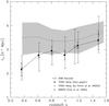 |
Fig. 11 Comparison of the correlation lengths as a function of redshift. The filled triangles with error bars are VVDS-Deep measurements while the dashed curve and associated shaded area correspond to the correlation length and error from the Omocks. We also report in this figure the previous VVDS-Deep measurements by Le Fèvre et al. (2005b) (crosses) and the one obtained by Coil et al. (2004) in the DEEP2 survey (open square). |
The clustering evolution of the global population of galaxies in the VVDS-Deep has been measured by Le Fèvre et al. (2005b) in the six redshift intervals from z = 0.2 to z = 2.1 previously defined. We update their measurements using the more accurate method described in the previous section. The wp(rp) measurements are shown in Fig. 10 along with the mean wp(rp) among the SAM Omocks samples. We fit the wp(rp) with power laws and provide the best-fitted parameters r0 and γ in Tables 1 and 2 for both the VVDS-Deep and the SAM. We compare the measured correlation lengths in Fig. 11. This figure shows that our measurements agree very well within the uncertainties with those previously obtained by Le Fèvre et al. (2005b) for the same field, as well as with results from the DEEP2 survey (Coil et al. 2004).
We recall that for all clustering comparisons, we use model predictions computed from the Omocks using the same method adopted for the VVDS-Deep data. Figure 10 shows that, when comparing Omocks (solid curves) and Cmocks (dashed curves) measurements, one find a non-negligible bias in the estimation of wp(rp) on small scales at z < 0.7. As already pointed out by Le Fèvre et al. (2005b), here the incompleteness effects are enhanced by the small volume and by the small number of objects in the observed samples at these redshifts. This emphasises the importance (and the necessity) to include detailed observational selection functions and biases in the mock samples in order to carry out a fair comparison between observational measurements and model predictions.
At z < 1.1, the SAM predicts on average a higher clustering amplitude than measured in the VVDS-Deep, while the slopes of the predicted and observed correlation functions are similar. In addition, while the correlation length in the VVDS-Deep increases slightly with increasing redshift, the model predicts a roughly constant correlation length over all the redshift range probed by the observations. Some evolution of the overall clustering is expected, because by selecting galaxies at increasing redshift in a magnitude-limited sample, we probe intrinsically more luminous galaxies on average. Observations show that brighter galaxies are more strongly clustered than their fainter counterparts (e.g. Norberg et al. 2001; Zehavi et al. 2005; Pollo et al. 2006; Coil et al. 2006). We explicitly show in the right panels of Fig. 7 and in Tables 1 and 2 that we indeed select intrinsically brighter galaxies with increasing redshift, both in the VVDS-Deep and the SAM. The relatively constant amplitude of the predicted correlation function suggests the absence (or a very weak) luminosity dependence of galaxy clustering in the model (see also Li et al. 2007; Kim et al. 2009a). We study this aspect in more detail in Paper II, where we measure the clustering of galaxies with different luminosities in the model and compare them with VVDS-Deep observations.
At z > 1.1, Fig. 10 shows that, although the overall amplitude of the predicted galaxy correlation function is similar to that measured, the model predicts a shallower correlation function than observed. The difference in slope and in shape of the correlation function can be interpreted within the framework of Halo Occupation Distribution models (e.g. Cooray & Sheth 2002). In this framework, the galaxy correlation function is the sum of two contributions, one dominating the smaller scales that characterises the clustering of galaxies residing in the same halo (the 1-halo term), and a large-scale contribution, which characterises the clustering of galaxies belonging to different haloes (the 2-halo term). At z > 1.1, the “bump” of the correlation function observed on scales smaller than or of the order of the typical halo radius (1–2 h-1 Mpc) in the VVDS-Deep, suggests that these galaxies are on average hosted by relatively massive haloes, with relatively large virial radii (e.g. Abbas et al. 2010). The model predicts instead a rather weak 1-halo term, which implies the presence of relatively few satellite galaxies. Satellite galaxies are defined as the galaxies residing within the virial radii of haloes that are not associated with their centres. The amplitude of the 1-halo term is directly linked to the amount of central-satellite and satellite-satellite pairs, and in turn to the abundance of satellite galaxies in their host haloes (e.g. Benson et al. 2000; Berlind et al. 2003; Kravtsov et al. 2004). We have previously shown that at z > 1.1 the model galaxy population is dominated by blue galaxies. Therefore, the small-scale shape of the correlation function predicted by the SAM at these redshifts, suggests that model galaxies are more likely to be blue central galaxies in low-mass haloes rather than blue or red satellites in more massive haloes, in contrast with what appears to be the case in the VVDS-Deep data.
It is worth noting that the Millennium Run simulation was carried out adopting a WMAP 1 cosmology, with a normalisation of the power spectrum of σ8 = 0.9. The most recent and accurate measurements favour instead a lower value of σ8 ≃ 0.81 (Komatsu et al. 2009, 2010). The value of σ8 has a non negligible influence on the amplitude of the dark matter correlation function, and in turn to that of galaxies. To quantify the effect on SAM clustering predictions, we convert the correlation functions in the SAM to those expected assuming the more recent value of σ8. To do so, we multiply the SAM wp(rp) by the ratio of the non-linear projected correlation function of mass for σ8 = 0.81 to that for σ8 = 0.9. We keep all the other cosmological parameters identical. We use the Smith et al. (2003) analytical prescription for the non-linear mass power spectrum, which we Fourier transform to obtain the correlation function. With this procedure, we assume a purely gravitational clustering evolution and do not account for a possible dependence of galaxy bias on σ8. This is, however, found to be weak in simulations (Wang et al. 2008). By rescaling the SAM projected correlation functions to σ8 = 0.81, we lower the amplitude of the predicted wp(rp) on all scales and obtain the dotted curves in Figs. 10 and 12. While this tends to improve the agreement between model predictions and observations, there are still some differences, in particular regarding the shape of the correlation functions on small scales.
4.3. Colour-dependent galaxy clustering
When selecting galaxies at 17.5 < I < 24 in the redshift interval 0.2 < z < 2, we probe an evolving mix of galaxy luminosities and colours (e.g. Le Fèvre et al. 2005b; Ilbert et al. 2005; Zucca et al. 2006; Franzetti et al. 2007). As a consequence, the clustering of these galaxies should reflect the average clustering of the different galaxy sub-populations at the different redshifts. In order to better understand the discrepancies found between the global clustering measured from VVDS-Deep data and that predicted by the model, we compare the clustering of two sub-sets of galaxies, red and blue ones, classified according to their bimodal colour distribution.
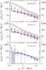 |
Fig. 12 Colour-dependent projected correlation functions in three redshift intervals from z = 0.2 to z = 2.1, both observed in the VVDS-Deep and predicted by the SAM. In each panel, the filled circles (red galaxies) and filled squares (blue galaxies) correspond to VVDS-Deep measurements, while the dashed curves and associated shaded areas correspond to the mean and the 1σ dispersion among the Omocks. The dotted curves are the mean wp(rp) obtained by rescaling the predicted correlations function to σ8 = 0.81 as described in Sect. 4.2. In all panels, both for VVDS-Deep and SAM galaxies, the wp(rp) with higher global amplitude corresponds to that of red galaxies. |
To keep a significant number of galaxies in each redshift interval, we used only 3 intervals between z = 0.2 and z = 2.1 in this part of the analysis. We do not consider any sample of red galaxies above z = 1.1, as the small number of objects prevents us from obtaining a robust wp(rp) measurement at these redshifts. Figures 12 and 13 show the projected correlation functions and the correlation lengths measured in the SAM and in the VVDS-Deep data for red and blue galaxies. The measurements from VVDS-Deep are consistent with those obtained from the same sample by Meneux et al. (2006), as well as with those obtained from the DEEP2 sample by Coil et al. (2004). We note that these two studies adopt different colour criteria to define blue and red galaxies and that the two surveys have different observational strategies. In particular, the DEEP2 survey selects galaxies brighter than those in the VVDS-Deep, which explains the slightly larger observed correlation lengths in the DEEP2 survey (see Le Fèvre et al. 2005b, for a detailed discussion).
We find that the correlation functions of blue galaxies in the model are in quite good agreement with VVDS-Deep measurements. In contrast, red model galaxies show a much stronger clustering on all scales. This suggests that the stronger clustering predicted by the SAM for the entire sample is due to the very strong clustering of red galaxies. As for the redshift trend, both VVDS-Deep observations and SAM predictions show a rather similar evolution over the redshift interval probed. The correlation length of red SAM galaxies is, however, much larger than observed and in fact similar to that observed for extremely red objects in the real Universe (e.g., Daddi et al. 2003).
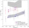 |
Fig. 13 Comparison of the correlation lengths of red and blue galaxies as a function of redshift. The filled symbols with error bars are VVDS-Deep measurements while the dashed curves and associated shaded areas correspond to the correlation lengths and errors in the Omocks. We also report previous VVDS-Deep measurements by Meneux et al. (2006) as well as those of Coil et al. (2004) from DEEP2 survey, both using different colour criteria. We refer the reader to the inset for the detail of the plotted symbols. |
As explained earlier, we have used different rest-frame B − I colour cuts to define red and blue galaxies in the model and in the observations. One may argue that the higher clustering amplitude observed for SAM red galaxies could be due to the redder colour cut applied to select the two populations, redder galaxies being expected to be more strongly clustered. To test this possibility we measure the clustering strength of red galaxies in the VVDS-Deep using the same colour cut used in the SAM, i.e. (B − I)cut = 1.3. In this way, we isolate in the VVDS-Deep sample red galaxies which have the same rest-frame B − I colour distribution than red model galaxies. As shown in Fig. 13, we find that these galaxies in the VVDS-Deep show a higher clustering amplitude than those selected with B − I > 0.95. However, the SAM clustering remains significantly stronger, demonstrating that red model galaxies are intrinsically more clustered than observed in the VVDS-Deep.
When studying the shape of the projected correlation functions in more detail, one finds that blue SAM galaxies are characterised by a shallower correlation function than VVDS-Deep galaxies, in particular on small scales. Within the HOD framework, this implies a weaker 1-halo term that can be interpreted as a lack of blue satellite galaxies in the SAM. In contrast, red model galaxies exhibit a correlation function which is significantly steeper and higher than observed. Here, the very prominent 1-halo term may be due to an overabundance of red satellite galaxies. Similarly, Coil et al. (2008) find an absence of “Finger of God” (FoG, Jackson 1972) in the correlation function of blue model galaxies at z ≃ 1 at variance with red model galaxies, which have a very strong FoG. The FoG effect is associated with the infall of satellite galaxies inside haloes and its strength is related to the abundance of satellite galaxies (e.g. Slosar et al. 2006). These results suggest that in the real Universe, (at least part of) the red satellites likely evolve less rapidly than in the model, and remain in the blue tail of the colour distribution for a longer time scale. This could adjust the different small-scale clustering behaviours of blue and red SAM and VVDS-Deep galaxies, but would not affect significantly the amplitude of the correlation functions.
To better see the impact of an overabundance of satellites on the clustering of galaxies, we randomly remove from the SAM mock samples 80% of the red satellites. The resulting galaxies correlation functions are shown in Fig. 14. This figure shows that, by excluding most of SAM red satellites, the amplitude of the correlation function of red galaxies is dramatically reduced, particularly on small scales. Model predictions obtained excluding 80 per cent of the red satellites are in quite good agreement with observational measurements but at 0.2 < z < 0.7, where there is still a significant difference between the amplitudes of the predicted and measured correlation functions. Similar conclusions have been reached while comparing the model to local measurements, e.g. Li et al. (2007) found that the match of the observed clustering in the local Universe to the previous version of the Munich model (Croton et al. 2006) can be improved by removing 30% of satellite galaxies in the model.
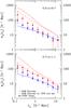 |
Fig. 14 Red and blue galaxy projected correlation functions in two redshift intervals from z = 0.2 to z = 1.1, both observed in the VVDS-Deep and predicted by the SAM (mean over Omocks samples). In each panel, the solid curves correspond to SAM mean predictions while the dashed ones to the resulting mean predictions while keeping only 20% of red satellite galaxies. The filled circles (red galaxies) and filled squares (blue galaxies) correspond to VVDS-Deep measurements. Both for the VVDS-Deep and the SAM, the wp(rp) with higher amplitude corresponds to that of red galaxies. The SAM correlation functions are rescaled to σ8 = 0.81 as described in Sect. 4.2. |
5. Summary and discussion
We have compared some of the basic high-redshift galaxy properties as measured in the VIMOS-VLT Deep Survey, to predictions from the Munich semi-analytical model. For this purpose, we have constructed 100 mock samples that accurately mimic the VVDS-Deep observational strategy. We have compared the magnitude counts, redshift distribution, colour bimodality, and galaxy clustering for galaxies with 17.5 < I < 24, probing a broad range of cosmic epochs from z = 2 to z = 0.2. We have demonstrated that, in order to cMNRAS, 375, 2arry out a fair comparison between model predictions and data, it is important to build “observed” mock samples that accurately reproduce the detailed selection function and biases of the observations.
We find that the Munich semi-analytical model reproduces reasonably well:
-
The magnitude counts in the u ∗ , g′, r′, i′, I and rest-frame B bands.
-
The shape of the redshift distribution at z < 1.8 for IAB < 24 galaxies, given the relatively large sample variance predicted by the model in the VVDS-Deep volume.
-
The global galaxy clustering at z > 0.8,
but fails to reproduce:
-
The magnitude counts in the z′ and rest-frame I bands.
-
The shape of the redshift distribution at z > 2 for IAB < 24 galaxies.
-
The rest-frame B − I colour distribution and its evolution with cosmic time since z ≃ 2.
-
The clustering strength of red galaxies.
-
The detailed small-scale clustering of both red and blue galaxies.
It is important to notice that for some of the predicted galaxy properties, there is a significant variance among different mock samples. For most of the observational measurements discussed in this study, we find that there are a few mock samples that are in good agreement with the data. On average, however, models deviate from observational measurements. In particular, for the colour distribution and the clustering of red galaxies, all mock samples differ from the VVDS-Deep measurements, and differences are larger than 3σ. None of the mock samples is able to reproduce all the VVDS-Deep measurements presented in this analysis, suggesting that the model failures highlighted above are not simply due to sample variance.
The discrepancies found between model predictions and VVDS-Deep observations extend to higher redshifts some of the model problems that have been previously emphasised from data-model comparisons in the local Universe. Although the blue population dominates in number density at all redshifts, the SAM tends to produce too many relatively bright red galaxies. As a consequence, the rest-frame I-band distribution is skewed towards bright magnitudes and the rest-frame B − I colour distribution towards the red. This excess of red galaxies is dominated by satellites, giving rise to a prominent 1-halo term in the correlation function of red model galaxies. In addition, the SAM underpredicts the fraction of blue satellite with respect to blue central galaxies as seen in the small-scale clustering of blue galaxies. It is important to mention that the excess of red satellite galaxies is not specific to the Munich semi-analytical model but is present in most of published semi-analytical models (Liu et al. 2010).
The excess of red and deficit of blue satellite galaxies in semi-analytical models are likely due to an over-efficient quenching of satellites, that transforms too many blue galaxies to red ones over a short time scale. In the models, star-forming blue galaxies become passive as a consequence of the infall of a galaxy onto a larger halo, or because of AGN feedback that suppresses star formation in massive central galaxies. An over-quenching of satellite galaxies can be produced by a too efficient strangulation, that instantaneously shuts off the star formation when a galaxy enters in a halo (Weinmann et al. 2006; Font et al. 2008; Kang & van den Bosch 2008; Kimm et al. 2009; Fontanot et al. 2009a). It is interesting to note that the truncation of gas accretion in satellite galaxies, and to a large extend of star formation, is also found to be less abrupt in smoothed particle hydrodynamics simulations (Cattaneo et al. 2007; Saro et al. 2010). This would help to explain the difference in the rest-frame colour distribution between models and data, but cannot explain the very strong intrinsic clustering of red galaxies. As recently pointed out by Kim et al. (2009a), Wetzel & White (2010), and Liu et al. (2010), the problem might lie in a poor treatment of satellite mergers and disruption. In fact, most of current semi-analytical models, including that used in this study, do not account for tidal stripping of satellite galaxies (but see Benson et al. 2002; Monaco et al. 2007). This can influence significantly the predicted clustering signal, and has been shown to affect also the predicted galaxy intrinsic colour distribution and stellar mass function (Yang et al. 2009). We study these aspects in more details in Paper II where we specifically relate the predicted galaxy clustering as a function of luminosity and colour to the halo occupation predicted by the model.
Acknowledgments
S.D.L.T. acknowledges financial support from ASI under contract ASI/COFIS/WP3110 I/026/07/0. G.D.L. acknowledges financial support from the European Research Council under the European Community’s Seventh Framework Programme (FP7/2007-2013)/ERC grant agreement No. 202781. A.P. was financed by the research grants of the Polish Ministry of Science PBZ/MNiSW/07/2006/34A and N N203 512938. This research has been developed within the framework of the VVDS consortium. This work has been partially supported by the CNRS-INSU and its Programme National de Cosmologie (France), and by INAF grant PRIN-INAF 2007. The VLT-VIMOS observations have been carried out on guaranteed time (GTO) allocated by the European Southern Observatory (ESO) to the VIRMOS consortium, under a contractual agreement between the Centre National de la Recherche Scientifique of France, heading a consortium of French and Italian institutes, and ESO, to design, manufacture and test the VIMOS instrument.
References
- Abbas, U., de la Torre, S., Le Fèvre, O., et al. 2010, MNRAS, 406, 1306 [NASA ADS] [Google Scholar]
- Arnouts, S., Walcher, C. J., Le Fèvre, O., et al. 2007, A&A, 476, 137 [NASA ADS] [CrossRef] [EDP Sciences] [Google Scholar]
- Bardelli, S., Zucca, E., Bolzonella, M., et al. 2009, A&A, 495, 431 [NASA ADS] [CrossRef] [EDP Sciences] [Google Scholar]
- Benson, A. J., Baugh, C. M., Cole, S., Frenk, C. S., & Lacey, C. G. 2000, MNRAS, 316, 107 [NASA ADS] [CrossRef] [Google Scholar]
- Benson, A. J., Lacey, C. G., Baugh, C. M., Cole, S., & Frenk, C. S. 2002, MNRAS, 333, 156 [NASA ADS] [CrossRef] [Google Scholar]
- Berlind, A. A., Weinberg, D. H., Benson, A. J., et al. 2003, ApJ, 593, 1 [NASA ADS] [CrossRef] [Google Scholar]
- Blaizot, J., Wadadekar, Y., Guiderdoni, B., et al. 2005, MNRAS, 360, 159 [NASA ADS] [CrossRef] [Google Scholar]
- Bottini, D., Garilli, B., Maccagni, D., et al. 2005, PASP, 117, 996 [NASA ADS] [CrossRef] [Google Scholar]
- Bower, R. G., Benson, A. J., Malbon, R., et al. 2006, MNRAS, 370, 645 [NASA ADS] [CrossRef] [Google Scholar]
- Bundy, K., Ellis, R. S., & Conselice, C. J. 2005, ApJ, 625, 621 [NASA ADS] [CrossRef] [Google Scholar]
- Cattaneo, A., Blaizot, J., Weinberg, D. H., et al. 2007, MNRAS, 377, 63 [NASA ADS] [CrossRef] [Google Scholar]
- Cimatti, A., Daddi, E., & Renzini, A. 2006, A&A, 453, L29 [NASA ADS] [CrossRef] [EDP Sciences] [Google Scholar]
- Coil, A. L., Davis, M., Madgwick, D. S., et al. 2004, ApJ, 609, 525 [NASA ADS] [CrossRef] [Google Scholar]
- Coil, A. L., Newman, J. A., Cooper, M. C., et al. 2006, ApJ, 644, 671 [NASA ADS] [CrossRef] [Google Scholar]
- Coil, A. L., Newman, J. A., Croton, D., et al. 2008, ApJ, 672, 153 [NASA ADS] [CrossRef] [Google Scholar]
- Colless, M., Dalton, G., Maddox, S., et al. 2001, MNRAS, 328, 1039 [NASA ADS] [CrossRef] [Google Scholar]
- Cooray, A., & Sheth, R. 2002, Phys. Rep., 372, 1 [NASA ADS] [CrossRef] [Google Scholar]
- Coupon, J., Ilbert, O., Kilbinger, M., et al. 2009, A&A, 500, 981 [NASA ADS] [CrossRef] [EDP Sciences] [Google Scholar]
- Cowie, L. L., Songaila, A., Hu, E. M., & Cohen, J. G. 1996, AJ, 112, 839 [Google Scholar]
- Croton, D. J., Springel, V., White, S. D. M., et al. 2006, MNRAS, 365, 11 [NASA ADS] [CrossRef] [Google Scholar]
- Daddi, E., Röttgering, H. J. A., Labbé, I., et al. 2003, ApJ, 588, 50 [NASA ADS] [CrossRef] [Google Scholar]
- Davis, M., Faber, S. M., Newman, J., et al. 2003, in Proc. SPIE 4834, ed. P. Guhathakurta, 161 [Google Scholar]
- de la Torre, S., Le Fèvre, O., Arnouts, S., et al. 2007, A&A, 475, 443 [NASA ADS] [CrossRef] [EDP Sciences] [Google Scholar]
- de la Torre, S., Le Fèvre, O., Porciani, C., et al. 2010, MNRAS, in press [arXiv:0911.2252] [Google Scholar]
- De Lucia, G. 2009, in American Institute of Physics Conf. Ser., ed. G. Giobbi, A. Tornambe, G. Raimondo, M. Limongi, L. A. Antonelli, N. Menci, & E. Brocato, 1111, 3 [Google Scholar]
- De Lucia, G., & Blaizot, J. 2007, MNRAS, 375, 2 [NASA ADS] [CrossRef] [Google Scholar]
- De Lucia, G., Kauffmann, G., & White, S. D. M. 2004, MNRAS, 349, 1101 [NASA ADS] [CrossRef] [Google Scholar]
- Dickinson, M., Giavalisco, M., & The Goods Team. 2003, in The Mass of Galaxies at Low and High Redshift, ed. R. Bender, & A. Renzini, 324 [Google Scholar]
- Fisher, K. B., Davis, M., Strauss, M. A., Yahil, A., & Huchra, J. P. 1994, MNRAS, 267, 927 [NASA ADS] [CrossRef] [Google Scholar]
- Font, A. S., Bower, R. G., McCarthy, I. G., et al. 2008, MNRAS, 389, 1619 [NASA ADS] [CrossRef] [Google Scholar]
- Fontanot, F., De Lucia, G., Monaco, P., Somerville, R. S., & Santini, P. 2009a, MNRAS, 397, 1776 [NASA ADS] [CrossRef] [Google Scholar]
- Fontanot, F., Somerville, R. S., Silva, L., Monaco, P., & Skibba, R. 2009b, MNRAS, 392, 553 [NASA ADS] [CrossRef] [Google Scholar]
- Franzetti, P., Scodeggio, M., Garilli, B., et al. 2007, A&A, 465, 711 [NASA ADS] [CrossRef] [EDP Sciences] [Google Scholar]
- Gavazzi, G., Pierini, D., & Boselli, A. 1996, A&A, 312, 397 [NASA ADS] [Google Scholar]
- Goranova, Y., Hudelot, P., Magnard, F., et al. 2009, The CFHTLS T0006 Release, http://terapix.iap.fr/cplt/table_syn_T0006.html [Google Scholar]
- Ilbert, O., Tresse, L., Zucca, E., et al. 2005, A&A, 439, 863 [NASA ADS] [CrossRef] [EDP Sciences] [Google Scholar]
- Ilbert, O., Salvato, M., Le Floc’h, E., et al. 2010, ApJ, 709, 644 [NASA ADS] [CrossRef] [Google Scholar]
- Iovino, A., McCracken, H. J., Garilli, B., et al. 2005, A&A, 442, 423 [NASA ADS] [CrossRef] [EDP Sciences] [Google Scholar]
- Jackson, J. C. 1972, MNRAS, 156, 1P [Google Scholar]
- Kang, X., & van den Bosch, F. C. 2008, ApJ, 676, L101 [NASA ADS] [CrossRef] [Google Scholar]
- Kauffmann, G., & Haehnelt, M. 2000, MNRAS, 311, 576 [NASA ADS] [CrossRef] [Google Scholar]
- Kim, H., Baugh, C. M., Cole, S., Frenk, C. S., & Benson, A. J. 2009a, MNRAS, 400, 1527 [NASA ADS] [CrossRef] [Google Scholar]
- Kim, J., Park, C., Gott, J. R., & Dubinski, J. 2009b, ApJ, 701, 1547 [NASA ADS] [CrossRef] [Google Scholar]
- Kimm, T., Somerville, R. S., Yi, S. K., et al. 2009, MNRAS, 394, 1131 [NASA ADS] [CrossRef] [Google Scholar]
- Kitzbichler, M. G., & White, S. D. M. 2007, MNRAS, 376, 2 [NASA ADS] [CrossRef] [Google Scholar]
- Komatsu, E., Dunkley, J., Nolta, M. R., et al. 2009, ApJS, 180, 330 [NASA ADS] [CrossRef] [Google Scholar]
- Komatsu, E., Smith, K. M., Dunkley, J., et al. 2010, ApJS, in press [arXiv:1001.4538] [Google Scholar]
- Kravtsov, A. V., Berlind, A. A., Wechsler, R. H., et al. 2004, ApJ, 609, 35 [NASA ADS] [CrossRef] [Google Scholar]
- Landy, S. D., & Szalay, A. S. 1993, ApJ, 412, 64 [NASA ADS] [CrossRef] [Google Scholar]
- Le Fèvre, O., Saisse, M., Mancini, D., et al. 2003, in Proc. SPIE 4841, ed. M. Iye, & A. F. M. Moorwood, 1670 [Google Scholar]
- Le Fèvre, O., Vettolani, G., Paltani, S., et al. 2004, A&A, 428, 1043 [NASA ADS] [CrossRef] [EDP Sciences] [Google Scholar]
- Le Fèvre, O., Vettolani, G., Garilli, B., et al. 2005a, A&A, 439, 845 [NASA ADS] [CrossRef] [EDP Sciences] [Google Scholar]
- Le Fèvre, O., Guzzo, L., Meneux, B., et al. 2005b, A&A, 439, 877 [NASA ADS] [CrossRef] [EDP Sciences] [Google Scholar]
- Leauthaud, A., Massey, R., Kneib, J.-P., et al. 2007, ApJS, 172, 219 [NASA ADS] [CrossRef] [Google Scholar]
- Li, C., Kauffmann, G., Jing, Y. P., et al. 2006, MNRAS, 368, 21 [NASA ADS] [CrossRef] [Google Scholar]
- Li, Y., Mo, H. J., van den Bosch, F. C., & Lin, W. P. 2007, MNRAS, 379, 689 [NASA ADS] [CrossRef] [Google Scholar]
- Lilly, S. J., Le Fèvre, O., Renzini, A., et al. 2007, ApJS, 172, 70 [NASA ADS] [CrossRef] [Google Scholar]
- Liu, L., Yang, X., Mo, H. J., van den Bosch, F. C., & Springel, V. 2010, ApJ, 712, 734 [NASA ADS] [CrossRef] [Google Scholar]
- McCracken, H. J., Radovich, M., Bertin, E., et al. 2003, A&A, 410, 17 [NASA ADS] [CrossRef] [EDP Sciences] [Google Scholar]
- McCracken, H. J., Peacock, J. A., Guzzo, L., et al. 2007, ApJS, 172, 314 [NASA ADS] [CrossRef] [Google Scholar]
- Meneux, B., Le Fèvre, O., Guzzo, L., et al. 2006, A&A, 452, 387 [NASA ADS] [CrossRef] [EDP Sciences] [Google Scholar]
- Meneux, B., Guzzo, L., Garilli, B., et al. 2008, A&A, 478, 299 [NASA ADS] [CrossRef] [EDP Sciences] [Google Scholar]
- Meneux, B., Guzzo, L., de la Torre, S., et al. 2009, A&A, 505, 463 [NASA ADS] [CrossRef] [EDP Sciences] [Google Scholar]
- Metcalfe, N., Shanks, T., Campos, A., McCracken, H. J., & Fong, R. 2001, MNRAS, 323, 795 [NASA ADS] [CrossRef] [Google Scholar]
- Monaco, P., Fontanot, F., & Taffoni, G. 2007, MNRAS, 375, 1189 [NASA ADS] [CrossRef] [Google Scholar]
- Norberg, P., Baugh, C. M., Hawkins, E., et al. 2001, MNRAS, 328, 64 [NASA ADS] [CrossRef] [Google Scholar]
- Norberg, P., Baugh, C. M., Gaztañaga, E., & Croton, D. J. 2009, MNRAS, 396, 19 [NASA ADS] [CrossRef] [Google Scholar]
- Peebles, P. J. E. 1980, The large-scale structure of the universe (Princeton University Press), 435 [Google Scholar]
- Pollo, A., Meneux, B., Guzzo, L., et al. 2005, A&A, 439, 887 [NASA ADS] [CrossRef] [EDP Sciences] [Google Scholar]
- Pollo, A., Guzzo, L., Le Fèvre, O., et al. 2006, A&A, 451, 409 [NASA ADS] [CrossRef] [EDP Sciences] [Google Scholar]
- Porciani, C., & Giavalisco, M. 2002, ApJ, 565, 24 [NASA ADS] [CrossRef] [Google Scholar]
- Postman, M., Lauer, T. R., Szapudi, I., & Oegerle, W. 1998, ApJ, 506, 33 [NASA ADS] [CrossRef] [Google Scholar]
- Pozzetti, L., Bolzonella, M., Lamareille, F., et al. 2007, A&A, 474, 443 [NASA ADS] [CrossRef] [EDP Sciences] [Google Scholar]
- Riess, A. G., Filippenko, A. V., Challis, P., et al. 1998, AJ, 116, 1009 [NASA ADS] [CrossRef] [Google Scholar]
- Saro, A., De Lucia, G., Borgani, S., & Dolag, K. 2010, MNRAS, 406, 729 [NASA ADS] [Google Scholar]
- Slosar, A., Seljak, U., & Tasitsiomi, A. 2006, MNRAS, 366, 1455 [NASA ADS] [CrossRef] [Google Scholar]
- Smith, R. E., Peacock, J. A., Jenkins, A., et al. 2003, MNRAS, 341, 1311 [NASA ADS] [CrossRef] [Google Scholar]
- Spergel, D. N., Verde, L., Peiris, H. V., et al. 2003, ApJS, 148, 175 [NASA ADS] [CrossRef] [Google Scholar]
- Springel, V., White, S. D. M., Tormen, G., & Kauffmann, G. 2001, MNRAS, 328, 726 [Google Scholar]
- Springel, V., White, S. D. M., Jenkins, A., et al. 2005, Nature, 435, 629 [NASA ADS] [CrossRef] [PubMed] [Google Scholar]
- Tegmark, M., Strauss, M. A., Blanton, M. R., et al. 2004, Phys. Rev. D, 69, 103501 [CrossRef] [Google Scholar]
- Tresse, L., Ilbert, O., Zucca, E., et al. 2007, A&A, 472, 403 [NASA ADS] [CrossRef] [EDP Sciences] [Google Scholar]
- Wang, J., De Lucia, G., Kitzbichler, M. G., & White, S. D. M. 2008, MNRAS, 384, 1301 [NASA ADS] [CrossRef] [Google Scholar]
- Weinberg, D. H., Davé, R., Katz, N., & Hernquist, L. 2004, ApJ, 601, 1 [NASA ADS] [CrossRef] [Google Scholar]
- Weinmann, S. M., van den Bosch, F. C., Yang, X., & Mo, H. J. 2006, MNRAS, 366, 2 [NASA ADS] [CrossRef] [Google Scholar]
- Wetzel, A. R., & White, M. 2010, MNRAS, 403, 1072 [NASA ADS] [CrossRef] [Google Scholar]
- White, S. D. M., & Frenk, C. S. 1991, ApJ, 379, 52 [NASA ADS] [CrossRef] [Google Scholar]
- Yang, X., Mo, H. J., & van den Bosch, F. C. 2009, ApJ, 693, 830 [NASA ADS] [CrossRef] [Google Scholar]
- York, D. G., Adelman, J., Anderson, Jr., J. E., et al. 2000, AJ, 120, 1579 [Google Scholar]
- Zehavi, I., Weinberg, D. H., Zheng, Z., et al. 2004, ApJ, 608, 16 [NASA ADS] [CrossRef] [Google Scholar]
- Zehavi, I., Zheng, Z., Weinberg, D. H., et al. 2005, ApJ, 630, 1 [Google Scholar]
- Zucca, E., Ilbert, O., Bardelli, S., et al. 2006, A&A, 455, 879 [NASA ADS] [CrossRef] [EDP Sciences] [Google Scholar]
All Tables
Definition and mean properties of the Munich semi-analytical model Cmocks samples.
All Figures
|
Fig. 1 Fraction of the number of galaxy with secure redshift (flag 2 to 9) over the total number of spectroscopic targets in the VVDS-Deep as a function of the I apparent magnitude (histogram). The solid curve is the average fraction over the Omocks samples. |
| In the text | |
|
Fig. 2 Angular distribution of galaxies in the VVDS-Deep (left) and in the Omocks sample 1 (right). The galaxies are shown with the dots and the background coloured areas encode the surface density of objects. The solid contours encompass the regions discarded by the photometric mask. |
| In the text | |
|
Fig. 3 Comparison of the magnitude counts in the VDIS I-band with SAM predictions and previously reported measurements by Postman et al. (1998) in the KPNO survey, Leauthaud et al. (2007) in the COSMOS-ACS field, and Metcalfe et al. (2001) in the Hubble Deep Field-North & South. The VVDS-Deep counts are shown with the empty squares and the error bars correspond to their associated Poisson errors. The solid curve and associated shaded areas are respectively the mean and the 1σ, 2σ, and 3σ field-to-field dispersions among Cmocks samples. |
| In the text | |
|
Fig. 4 Comparison of the magnitude counts in the CFHTLS u ∗ , g′, r′, i′, z′ optical bands with SAM predictions for 17.5 < I < 24 galaxies. The CFHTLS counts are shown with the squares and the error bars correspond to their Poisson errors. The curves and associated shaded areas are respectively the mean and the 1σ, 2σ, and 3σ field-to-field dispersions among the Cmocks samples. SAM predictions are for samples explicitly cut at I = 24, while CFHTLS counts extend above this limit. All galaxies with I < 17.5 have been removed from the counts. |
| In the text | |
|
Fig. 5 Comparison of the VVDS-Deep with the SAM redshift distributions for 17.5 < IAB < 24 galaxies. The VVDS-Deep N(z), while including only flag 2 to 9 galaxies, is shown with the solid thin histogram. The thick histogram corresponds to the corrected N(z) in the VVDS-Deep when accounting for the observational biases of the survey (see text for details). The solid curve and associated shaded area are the mean and the 1σ field-to-field dispersion among the Omocks, while the dotted curve is the mean prediction of the Cmocks. |
| In the text | |
|
Fig. 6 Comparison of the rest-frame B-band (right panels) and I-band (left panels) distributions in six magnitude-limited samples from z = 0.2 to z = 2.1. The histograms are VVDS-Deep measurements while the curves and associated shaded areas correspond to the mean and the 1σ field-to-field dispersion among the Omocks samples. The dashed curves are the mean distribution in the Omocks without including dust extinction in the model, while the dotted ones are the mean predictions of the Cmocks. |
| In the text | |
|
Fig. 7 Comparison of the rest-frame B − I distribution in six magnitude-limited samples from z = 0.2 to z = 2.1. In each panel, the histogram corresponds to the VVDS-Deep measurement while the curve and associated shaded area correspond to the mean and the 1σ field-to-field dispersion among the Omocks samples. The dashed curves are the mean distribution in the Omocks without including dust extinction in the model, while the dotted ones are the mean predictions of the Cmocks. |
| In the text | |
|
Fig. 8 Total number and fraction of red (filled circles) and blue (filled squares) galaxies as a function of redshift in the VVDS-Deep and in the SAM. The symbols with error bars are the VVDS-Deep measurements while solid curves and associated shaded areas correspond to the predicted mean fractions and 1σ field-to-field dispersions among the Omocks. The dotted curves are the mean predictions of the Cmocks. In both upper and lower panel, higher curves and symbols correspond to blue galaxies. |
| In the text | |
|
Fig. 9 Mean projected correlation function at 0.7 < z < 1.1 for red (top curves), all (middle curves), and blue (bottom curves) galaxies in the Omocks (dashed curves) and Cmocks (solid curves) samples. The error bars correspond to the 1σ field-to-field dispersion among the mock samples. Omocks points have been slightly displaced along rp-axis to improve the clarity of the figure. |
| In the text | |
|
Fig. 10 Comparison of the projected correlation functions as a function of redshift. In each panel, the filled triangles with error bars correspond to VVDS-Deep measurements while the solid curve and associated shaded area correspond to the mean and the 1σ field-to-field dispersion among the Omocks samples. The dashed curves are the mean Cmocks predictions, while the dotted ones are the mean wp(rp) obtained by rescaling the predicted correlations function in the Omocks to σ8 = 0.81 as described in Sect. 4.2. |
| In the text | |
|
Fig. 11 Comparison of the correlation lengths as a function of redshift. The filled triangles with error bars are VVDS-Deep measurements while the dashed curve and associated shaded area correspond to the correlation length and error from the Omocks. We also report in this figure the previous VVDS-Deep measurements by Le Fèvre et al. (2005b) (crosses) and the one obtained by Coil et al. (2004) in the DEEP2 survey (open square). |
| In the text | |
|
Fig. 12 Colour-dependent projected correlation functions in three redshift intervals from z = 0.2 to z = 2.1, both observed in the VVDS-Deep and predicted by the SAM. In each panel, the filled circles (red galaxies) and filled squares (blue galaxies) correspond to VVDS-Deep measurements, while the dashed curves and associated shaded areas correspond to the mean and the 1σ dispersion among the Omocks. The dotted curves are the mean wp(rp) obtained by rescaling the predicted correlations function to σ8 = 0.81 as described in Sect. 4.2. In all panels, both for VVDS-Deep and SAM galaxies, the wp(rp) with higher global amplitude corresponds to that of red galaxies. |
| In the text | |
|
Fig. 13 Comparison of the correlation lengths of red and blue galaxies as a function of redshift. The filled symbols with error bars are VVDS-Deep measurements while the dashed curves and associated shaded areas correspond to the correlation lengths and errors in the Omocks. We also report previous VVDS-Deep measurements by Meneux et al. (2006) as well as those of Coil et al. (2004) from DEEP2 survey, both using different colour criteria. We refer the reader to the inset for the detail of the plotted symbols. |
| In the text | |
|
Fig. 14 Red and blue galaxy projected correlation functions in two redshift intervals from z = 0.2 to z = 1.1, both observed in the VVDS-Deep and predicted by the SAM (mean over Omocks samples). In each panel, the solid curves correspond to SAM mean predictions while the dashed ones to the resulting mean predictions while keeping only 20% of red satellite galaxies. The filled circles (red galaxies) and filled squares (blue galaxies) correspond to VVDS-Deep measurements. Both for the VVDS-Deep and the SAM, the wp(rp) with higher amplitude corresponds to that of red galaxies. The SAM correlation functions are rescaled to σ8 = 0.81 as described in Sect. 4.2. |
| In the text | |
Current usage metrics show cumulative count of Article Views (full-text article views including HTML views, PDF and ePub downloads, according to the available data) and Abstracts Views on Vision4Press platform.
Data correspond to usage on the plateform after 2015. The current usage metrics is available 48-96 hours after online publication and is updated daily on week days.
Initial download of the metrics may take a while.