| Issue |
A&A
Volume 524, December 2010
|
|
|---|---|---|
| Article Number | A68 | |
| Number of page(s) | 18 | |
| Section | Cosmology (including clusters of galaxies) | |
| DOI | https://doi.org/10.1051/0004-6361/201015271 | |
| Published online | 24 November 2010 | |
Mass profiles and c − MDM relation in X-ray luminous galaxy clusters
1
INAF, Osservatorio Astronomico di Bologna, via Ranzani 1,
40127
Bologna,
Italy
e-mail: This email address is being protected from spambots. You need JavaScript enabled to view it.
2
INFN, Sezione di Bologna, via le Berti Pichat 6/2,
40127
Bologna,
Italy
3
INAF, IASF, via Bassini 15, 20133
Milano,
Italy
4
Università degli Studi di Milano, Dip. di Fisica, via Celoria 16, 20133
Milano,
Italy
5
Department of Physics and Astronomy, University of
California, Irvine,
CA
92697-4575,
USA
Received:
24
June
2010
Accepted:
14
September
2010
Abstract
Context. Galaxy clusters represent valuable cosmological probes using tests that mainly rely on measurements of cluster masses and baryon fractions. X-ray observations represent one of the main tools for uncovering these quantities.
Aims. We aim to constrain the cosmological parameters Ωm and σ8 using the observed distribution of the both values of the concentrations and dark mass within R200 and of the gas mass fraction within R500.
Methods. We applied two different techniques to recover the profiles the gas and dark mass, described according to the Navarro, Frenk & White (1997, ApJ, 490, 493) functional form, of a sample of 44 X-ray luminous galaxy clusters observed with XMM-Newton in the redshift range 0.1−0.3. We made use of the spatially resolved spectroscopic data and of the PSF–deconvolved surface brightness and assumed that hydrostatic equilibrium holds between the intracluster medium and the gravitational potential. We evaluated several systematic uncertainties that affect our reconstruction of the X-ray masses.
Results. We measured the concentration c200,
the dark mass M200 and the gas mass fraction in all the
objects of our sample, providing the largest dataset of mass parameters for galaxy
clusters in the redshift range 0.1 − 0.3. We confirm that a tight correlation between
c200 and M200 is present and in
good agreement with the predictions from numerical simulations and previous observations.
When we consider a subsample of relaxed clusters that host a low entropy core, we measure
a flatter c − M relation with a total scatter that is
lower by 40 per cent. We conclude, however, that the slope of the
c − M relation cannot be reliably determined from the
fitting over a narrow mass range as the one considered in the present work. From the
distribution of the estimates of c200 and
M200, with associated statistical (15–25%) and systematic
(5–15%) errors, we used the predicted values from semi-analytic prescriptions calibrated
through N-body numerical runs and obtain 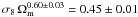 (at 2σ level, statistical only) for the subsample of the clusters where
the mass reconstruction has been obtained more robustly and
(at 2σ level, statistical only) for the subsample of the clusters where
the mass reconstruction has been obtained more robustly and  for the subsample of the 11 more relaxed LEC
objects. With the further constraint from the gas mass fraction distribution in our
sample, we break the degeneracy in the σ8 − Ωm
plane and obtain the best-fit values σ8 ≈ 1.0 ± 0.2
(0.83 ± 0.1 when the subsample of the more relaxed objects is considered) and
Ωm = 0.26 ± 0.02.
for the subsample of the 11 more relaxed LEC
objects. With the further constraint from the gas mass fraction distribution in our
sample, we break the degeneracy in the σ8 − Ωm
plane and obtain the best-fit values σ8 ≈ 1.0 ± 0.2
(0.83 ± 0.1 when the subsample of the more relaxed objects is considered) and
Ωm = 0.26 ± 0.02.
Conclusions. Analysis of the distribution of the c200 − M200 − fgas values represents a mature and competitive technique in the present era of precision cosmology, even though it needs more detailed analysis of the output of larger sets of cosmological numerical simulations to provide definitive and robust results.
Key words: galaxies: cluster: general / intergalactic medium / X-ray: galaxies: clusters / cosmology: observations / dark matter
Occhialini Fellow
© ESO, 2010
1. Introduction
The distribution of the total and baryonic mass in galaxy clusters is a fundamental
ingredient to validate the scenario of structure formation in a Cold Dark Matter (CDM)
Universe. Within this scenario, the massive virialized objects are powerful cosmological
tools able to constrain the fundamental parameters of a given CDM model. The
N-body simulations of structure formation in CDM models indicate that
dark matter halos aggregate with a typical mass density profile characterized by only
2 parameters, the concentration c and the scale radius
rs (e.g. Navarro et al. 1997, hereafter NFW). The product of these two quantities fixes the radius within
which the mean cluster density is 200 times the critical value at the cluster’s redshift
[i.e.
R200 = c200 × rs
and the cluster’s volume  is equal
to
M200/(200ρc,z),
where M200 is the cluster gravitating mass within
R200]. With this prescription, the structural properties of DM
halos from galaxies to galaxy clusters are dependent on the halo mass, with systems at
higher masses less concentrated. Moreover, the concentration depends upon the assembly
redshift (e.g. Bullock et al. 2001; Wechsler et al.
2002; Zhao et al. 2003; Li et al. 2007), which
happens to be later in cosmologies with lower matter density, Ωm, and lower
normalization of the linear power spectrum on scale of 8 h-1
Mpc, σ8, implying less concentrated DM halos of given mass. The
concentration – mass relation, and its evolution in redshift, is therefore a strong
prediction obtained from CDM simulations of structure formation and is quite sensitive to
the assumed cosmological parameters (NFW; Bullock et al. 2001; Eke et al. 2001; Dolag et al. 2004; Neto et al. 2007; Macciò et al. 2008). In this context,
NFW, Bullock et al. 2001 (with revision after Macciò
et al. 2008) and Eke et al. 2001 have provided simple and powerful models that match the predictions
from numerical simulations and allow comparison with the observational measurements.
is equal
to
M200/(200ρc,z),
where M200 is the cluster gravitating mass within
R200]. With this prescription, the structural properties of DM
halos from galaxies to galaxy clusters are dependent on the halo mass, with systems at
higher masses less concentrated. Moreover, the concentration depends upon the assembly
redshift (e.g. Bullock et al. 2001; Wechsler et al.
2002; Zhao et al. 2003; Li et al. 2007), which
happens to be later in cosmologies with lower matter density, Ωm, and lower
normalization of the linear power spectrum on scale of 8 h-1
Mpc, σ8, implying less concentrated DM halos of given mass. The
concentration – mass relation, and its evolution in redshift, is therefore a strong
prediction obtained from CDM simulations of structure formation and is quite sensitive to
the assumed cosmological parameters (NFW; Bullock et al. 2001; Eke et al. 2001; Dolag et al. 2004; Neto et al. 2007; Macciò et al. 2008). In this context,
NFW, Bullock et al. 2001 (with revision after Macciò
et al. 2008) and Eke et al. 2001 have provided simple and powerful models that match the predictions
from numerical simulations and allow comparison with the observational measurements.
Recent X-ray studies (Pointecouteau et al. 2005; Vikhlinin et al. 2006; Voigt & Fabian 2006; Zhang et al. 2006; Buote et al. 2007) have shown good agreement between observational constraints at low redshift and theoretical expectations. By fitting 39 systems in the mass range between early-type galaxies up to massive galaxy clusters, Buote et al. (2007) confirm with high significance that the concentration decreases with increasing mass, as predicted from CDM models, and require a σ8, the dispersion of the mass fluctuation within spheres of comoving radius of 8 h-1 Mpc, in the range 0.76 − 1.07 (99% confidence) definitely in contrast to the lower constraints obtained, for instance, from the analysis of the WMAP 3 years data. Since it is based upon a selection of the most relaxed systems, these results assumed a 10% upward early formation bias in the concentration parameter for relaxed halos. Using a sample of 34 massive, dynamically relaxed galaxy clusters resolved with Chandra in the redshift range 0.06 − 0.7, Schmidt & Allen (2007) highlight a possible tension between the observational constraints and the numerical predictions, in the sense that either the relation is steeper than previously expected or some redshift evolution has to be considered. Comerford & Natarajan (2007) compiled a large dataset of observed cluster concentration and masses, finding a normalization higher by at least 20 per cent than the results from simulations. In the sample, they use also strong lensing measurements of the concentration concluding that these are systematically larger than the ones estimated in the X-ray band, and 55 per cent higher, on average, than the rest of the cluster population. Recently, Wojtak & Łokas (2010) analyze kinematic data of 41 nearby (z < 0.1) relaxed objects and find a normalization of the concentration – mass relation fully consistent with the amplitude of the power spectrum σ8 estimated from WMAP1 data and within 1σ from the constraint obtained from WMAP5.
Sample of the galaxy clusters.
In this work, we use the results of the spectral analysis presented in Leccardi & Molendi (2008a) for a sample of 44 X-ray luminous galaxy clusters located in the redshift range 0.1 − 0.3 with the aim to (1) recover their total and gas mass profiles, (2) constraining the cosmological parameters σ8 and Ωm through the analysis of the measured distribution of c200, M200 and baryonic mass fraction in the mass range above 1014 M⊙. We note that this is the statistically largest sample for which this study has been carried on up to now between z = 0.1 and z = 0.3.
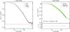 |
Fig. 1 (Left) Surface brightness profile in the 0.7−1.2 keV band (black filled circles) of Abell1835 compared with the profiles of the background components. The open diamonds show the count rate predicted from the background spectral model in the annulus 10–12 arcmin and rescaled for the mean vignetting correction of 0.472 at those radii: the instrumental component (NXB; green), the photon component (CXB + galactic foregrounds; blue) and the total background (sky + instrumental; red). The dashed lines show the background profiles that we have used in our analysis: the “photon” background (blue), which is constant and corresponds to the value in the outer annulus rescaled to the center, and the instrumental background profile (green), increasing with radius in order to consider the over-correction of this component. The red dashed line shows the total background that we have subtracted from our source plus background profile, with its associated one σ statistical error (red dotted lines) obtained with a Monte Carlo simulation. Note that the intensity of the background components and their relative contribution vary significantly from cluster to cluster. (Right) Example of the PSF-corrected background-subtracted surface brightness profile as obtained after the analysis outlined in Sect. 2.2. This example refers to Abell1835, one of the objects with the largest smearing effect due to the combination of the telescope’s PSF and the centrally peaked intrinsic profile. |
The outline of our work is the following. In Sect. 2, we describe the dataset of
XMM-Newton observations used in our analysis to recover the gas and total
mass profiles with the techniques presented in Sect. 3. In Sect. 4, we present a detailed
discussion of the main systematic uncertainties that affect our measurements. We investigate
the c200 − M200 relation in Sect. 5.
By using our measurements of c200 and
M200, we constrain the cosmological parameters
σ8 and Ωm, breaking the degeneracy between these
parameters by adding the further cosmological constraints from our estimates of the cluster
baryon fraction, as discussed in Sect. 6. We summarize our results and draw the conclusion
of the present study in Sect. 7. Throughout this work, if not otherwise stated, we plot and
tabulate values estimated by assuming a Hubble constant  km
s-1 Mpc-1 and Ωm = 1 − ΩΛ = 0.3, and quote
errors at the 68.3 per cent (1σ) level of confidence.
km
s-1 Mpc-1 and Ωm = 1 − ΩΛ = 0.3, and quote
errors at the 68.3 per cent (1σ) level of confidence.
We list here in alphabetic order, with the adopted acronyms, the work to which we will refer more often in the present study: Bullock et al. (2001 – B01); Dolag et al. (2004 – D04); Eke et al. (2001 – E01); Leccardi & Molendi (2008a – LM08); Macciò et al. (2008 – M08); Navarro et al. (1997 – NFW); Neto et al. (2007 – N07).
2. The dataset
Leccardi & Molendi (2008a) have retrieved from the XMM-Newton archive all observations of clusters available at the end of May 2007 (and performed before March 2005, when the CCD6 of EPIC-MOS1 was switched off) and satisfying the selection criteria to be hot (kT > 3.3 keV), at intermediate redshift (0.1 < z < 0.3), and at high galactic latitude (|b| > 20°). Upper and lower limits to the redshift range are determined, respectively, by the cosmological dimming effect and the size of the EPIC field of view (15′ radius). Out of 86 observations, 23 were excluded because they are highly affected by soft proton flares (see Table 1 in LM08) and have cleaned exposure time less than 16 ks when summing MOS1 and MOS2. Furthermore, 15 observations were excluded because they show evidence of recent and strong interactions (see Table 2 in LM08). The spectral analysis of the remaining 48 exposures, for a total of 44 clusters, is presented in LM08 and summarized in the next subsection. In Table 1, we present the list of the clusters analyzed in the present work.
2.1. Spatially resolved spectral analysis
We use gas temperature profiles measured by LM08. A detailed description of how the profiles were obtained and tested against systematic uncertainties can be found in their paper. Here we briefly review some of the most important points. Unlike most temperature estimates the one reported in LM08 have been secured by performing background modelling rather than background subtraction. Great care and considerable effort has gone into building an accurate model of the EPIC background, both in terms of its instrumental and cosmic components. Unfortunately the impossibility of performing an adequate monitoring of the pn instrumental background during source observation resulted in the exclusion of this detector from the analysis. Therefore, we adopt the measurements obtained from the two MOS instruments (M1 and M2, hereafter) independently in the following analysis.
The impact of small errors in the background estimates on temperature and normalization estimates was tested both by performing Monte-Carlo simulations (a-priori tests) and by checking how results varied for different choices of key parameters (a-posteriori tests). The detailed analysis allowed to track systematic errors and provide an error budget including both statistical and systematic uncertainties.
The two profiles have been analyzed both independently and after they were combined as described below. M1 and M2 are cross-calibrated to about 5% (Mateos et al. 2009). The largest discrepancy appears to be in the high energy range (above 4.5 keV), leading to a general tendency where M2 returns slightly softer spectra than M1. Since a similar comparison between M2 and pn shows that the latter returns even softer spectra, the M2 experiment may be viewed as returning spectra which are intermediate between M1 and pn in the 0.7 − 10 keV band. As consequence of that, a systematic shift between the M1 and M2 temperature profiles is present, meaning that an higher measurements is obtained with M1. This shift is not very sensitive to the value of the temperature, but instead manifests itself as a difference between M1 and M2 in the shape of the radial temperature profile. Using as reference the value of gas temperature measured with M2, we estimate the median deviation in the different radial bins to be 4.8% in the inner bin, 8.9% in the following 4 bins, 10% from the 5th bin upwards. The two profiles are then combined by a weighted mean and a further systematic error is added, as described in Leccardi & Molendi (2008a; see Sect. 5.3): i.e. 2, 3 and 5 per cent increases are considered at 0.3 < r/R180 < 0.36, 0.36 < r/R180 < 0.45 and r/R180 > 0.45, respectively. For this purpose, R180 as defined in Table 3 in Leccardi & Molendi (2008a) is considered. An error of the same amount is propagated in quadrature with the statistical error.
On the other hand, no significant effect is noticed when the values of the normalization of the thermal model K obtained from the two different instruments are compared. The combined profile is then the direct result of the weighted mean of the two estimates.
Unlike in LM08, where the focus was on the measure of the Tgas profile in outer regions, here we need to recover a detailed description of both the Tgas and surface brightness Sb profiles at large and small radii. A significant improvement compared to the treatment by LM08 has been the correction of the spectral mixing between different annuli caused by the finite PSF of the MOS instruments. We adopted the cross-talk modification of the ancillary region file (ARF) generation software (using the crossregionarf parameter of the argen task of SAS), treating the cross-talk contribution to the spectrum of a given annulus from a nearby annulus as an additional model component (see Snowden et al. 2008). This is a thermal model with parameters linked to the thermal spectrum fitted to the nearby annulus and associated to the appropriate ARF file of that region (i.e., the usual ARF familiar to X-ray astronomers). We found the correction to be important in particular to the first two annuli used in the analysis. The annuli have been therefore fitted jointly in XSPEC version 12 (Arnaud 1996), which allows to associate different models to different RMF and ARF files. A comparison of the values obtained with this modelling and the values quoted in Snowden et al. (2008) for the 16 clusters in common with our sample give results in agreement within the errors.
2.2. Analysis of the surface brightness profile
We extend the spectral analysis presented in LM08 with a spatial analysis of the combined exposure-corrected M1-M2 images.
We extract surface brightness profiles from MOS images in the energy band 0.7 − 1.2 keV, in order to keep the background as low as possible with respect to the source. For this reason, we avoid the intense fluorescent instrumental lines of Al (~1.5 keV) and Si (~1.8 keV) (LM08). To correct for the vignetting, we divide the images by the corresponding exposure maps. From the surface brightness profiles, we subtract the background that is estimated starting from the spectral modelling of the background components in the external ring 10–12 arcmin (see LM08 for details on the adopted models). We recall here that in the procedure of LM08 the normalizations of the background components are the only free parameters of the fit and that the galactic foreground emission, the cosmic X-ray background and the cosmic ray induced continuum give a significant contribution in the 0.7 − 1.2 keV energy range. The intensities of the background components in the annulus 10–12 arcmin are given by the count rates predicted by the best fit spectral model in this region. In order to associate errors to these count rates, we perform a simulation within XSPEC: we allow the normalizations of the background components to vary randomly within their errors, we obtain the count rates associated to this fake model and we iterate this procedure. The error on the level of the background components is the width of the distribution of the simulated count rates. Using these values in the outer annulus, we reconstruct the background profile at all radii. The “photon” components (CXB and galactic foreground) are affected by vignetting in the same way as the source photons and, therefore, dividing by the exposure map effectively corrects also these background components for the vignetting. In order to reconstruct the “photon” background profile, it is thus sufficient to rescale the count rate for the mean vignetting in the outer annulus (constant blue profile in Fig. 1). On the contrary, the instrumental background does not suffer from vignetting and, therefore, dividing the image by the exposure map “mis-corrects” this component. In order to consider this effect, we divide the corresponding count rate by the vignetting profile (that we derive from the exposure map in the 0.7 − 1.2 keV), obtaining the growing green curve in Fig. 1. The total background profile (red line in Fig. 1) is the sum of the photon (blue) and instrumental (green) profiles.
The surface brightness profiles Sb(r) have
been first extracted from the combined images and binned by requiring a fixed number of
200 counts in each radial bin to preserve all the spatial information available. After the
background subtraction, they have been corrected for the PSF smearing. For this purpose, a
sum of a cusped β-model and of a β-model (Cavaliere
& Fusco-Femiano 1978) with seven free
parameters, ![Mathematical equation: $f_m(r) = a_0 \times \left[ x_1^{-a_2} \times \left( 1+x_1^2 \right)^{0.5-3 a_3+a_2/2} +a_4 \left( 1+x_2^2 \right)^{0.5-3 a_6} \right]$](/articles/aa/full_html/2010/16/aa15271-10/aa15271-10-eq56.png) (with
x1 = r/a1
and
x2 = r/a2),
is convolved with the predicted PSF (Ghizzardi 2001) and fitted to the observed profile background-subtracted
Sb(r) to obtain the best-fit convolved
model
(with
x1 = r/a1
and
x2 = r/a2),
is convolved with the predicted PSF (Ghizzardi 2001) and fitted to the observed profile background-subtracted
Sb(r) to obtain the best-fit convolved
model  . Finally, to correct
Sb(r) for the PSF-convolution, we apply a
correction at each radius
. Finally, to correct
Sb(r) for the PSF-convolution, we apply a
correction at each radius  where
Sb(r) is measured equal to the ratio
where
Sb(r) is measured equal to the ratio
 . An example of the
results of the procedure is shown in Fig. 1. These
corrected profiles are, finally, used in the following analysis up to the radial limit,
Rsp, beyond which the ratio between the profile and the
error on it (including the estimated uncertainty on the measurement of the background) is
below 2.
. An example of the
results of the procedure is shown in Fig. 1. These
corrected profiles are, finally, used in the following analysis up to the radial limit,
Rsp, beyond which the ratio between the profile and the
error on it (including the estimated uncertainty on the measurement of the background) is
below 2.
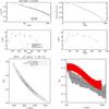 |
Fig. 2 Example of the results of the two analyses adopted for the mass reconstruction.
(Top and middle panels, left) Gas density profile as obtained
from the deprojection of the surface brightness profile compared to the one
recovered from the deprojection of the normalizations of the thermal model in the
spectral analysis; observed temperature profile with overplotted the best-fit model
(from Method 1). (Top and middle panels, right)
Data (diamonds) and models (dashed lines) of the projected gas density
squared and temperature (from Method 2). (Bottom, left)
Constraints in the rs − c
plane with the prediction (in green) obtained by imposing the relation
|

Results on the mass reconstruction.
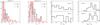 |
Fig. 3 (First 2 panels on the left) Relative errors on M200 (black) and c200 (red) estimated by the two methods. The median values are indicated by a dashed line. (3rd and 4th panel from left) Ratios between the best-fit result on the scale radius rs (3rd panel) and on R500 (4th panel) and outermost radius reached with the spatial analysis. |
Estimates of R200, R500 and the gas mass fraction.
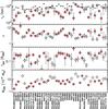 |
Fig. 4 Best-fit values of rs, c, gas mass fraction fgas at R500 and dark mass MDM within R200 as obtained from Method 1 (diamonds; the ones including red points indicate the objects where the condition (rs + ϵrs) < Rsp is satisfied by both methods. Rsp here plotted as horizontal line in the upper panel). |
3. Estimates of the mass profiles
We use the profiles of the spectroscopically determined ICM temperature and of the PSF-corrected surface brightness estimated, as described in the previous section, to recover the X-ray gas, the dark and the total mass profiles, under the assumptions of the spherical geometry distribution of the intracluster medium (ICM) and that the hydrostatic equilibrium holds between ICM and the underlying gravitational potential. We apply the two following different methods:
(Method 1) This technique is described in Ettori et al. (2002) and has been widely used to recover the mass profiles in recent X-ray studies of both observational (e.g. Morandi et al. 2007; Donnarumma et al. 2009, 2010) and simulated datasets (e.g. Rasia et al. 2006; Meneghetti et al. 2010) against which it has been thoroughly tested. We summarize here the algorithm adopted and how it uses the observed measurements. Starting from the X-ray surface brightness profile and the radially resolved spectroscopic temperature measurements, this method puts constraints on the parameters of the functional form describing the dark matter MDM, defined as the total mass minus the gas mass (we neglect the marginal contribution from the mass in stars that amounts to about 10–15% of the gas mass in massive systems – see, e.g., discussion in Ettori et al. 2009; Andreon 2010 –, and is here formally included in the MDM term). In the present work, we adopt a NFW profile:
 (1)where
x = r/rs,
(1)where
x = r/rs,
 is the critical density at the cluster’s
redshift z,
is the critical density at the cluster’s
redshift z, ![Mathematical equation: $H_z = H_0 \times \left[ \Omega_{\Lambda} +\Omega_{\rm m} (1+z)^3 \right]^{1/2}$](/articles/aa/full_html/2010/16/aa15271-10/aa15271-10-eq803.png) is the Hubble constant
at redshift z for an assumed flat Universe
(Ωm + ΩΛ = 1), and the relation
R200 = c200 × rs
holds. The two parameters
(rs,c200)
are constrained by minimizing a χ2 statistic defined as
is the Hubble constant
at redshift z for an assumed flat Universe
(Ωm + ΩΛ = 1), and the relation
R200 = c200 × rs
holds. The two parameters
(rs,c200)
are constrained by minimizing a χ2 statistic defined as
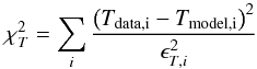 (2)where
the sum is done over the annuli of the spectral analysis;
Tdata are the either deprojected or observed temperature
measurements obtained in the spectral analysis; Tmodel are
either the three-dimensional or projected values of the estimates of
Tgas recovered from the inversion of the hydrostatic
equilibrium equation (see below) for a given gas density and total mass profiles;
ϵT is the error on the spectral
measurements. The gas density profile, ngas, is estimated
from the geometrical deprojection (Fabian et al. 1981; Kriss et al. 1983; McLaughlin
1999; Buote 2000; Ettori et al. 2002) of either
the measured X-ray surface brightness or the estimated normalization of the thermal
model fitted in the spectral analysis (see Fig. 2). In the present study, we consider the observed spectral values of the
temperature and evaluate Tmodel by projecting the
estimates of Tgas over the annuli adopted in the spectral
analysis accordingly to the recipe in Mazzotta et al. (2004) and using the gas density profile obtained from the deprojection of
the PSF-deconvolved surface brightness profile (see Sect. 2.2). We exclude the
deprojected data of the gas density within a cutoff radius of 50 kpc because the
influence of the central galaxy is expected to be not negligible, in particular for
strong low-entropy core systems. The values of Tgas are
then obtained from
(2)where
the sum is done over the annuli of the spectral analysis;
Tdata are the either deprojected or observed temperature
measurements obtained in the spectral analysis; Tmodel are
either the three-dimensional or projected values of the estimates of
Tgas recovered from the inversion of the hydrostatic
equilibrium equation (see below) for a given gas density and total mass profiles;
ϵT is the error on the spectral
measurements. The gas density profile, ngas, is estimated
from the geometrical deprojection (Fabian et al. 1981; Kriss et al. 1983; McLaughlin
1999; Buote 2000; Ettori et al. 2002) of either
the measured X-ray surface brightness or the estimated normalization of the thermal
model fitted in the spectral analysis (see Fig. 2). In the present study, we consider the observed spectral values of the
temperature and evaluate Tmodel by projecting the
estimates of Tgas over the annuli adopted in the spectral
analysis accordingly to the recipe in Mazzotta et al. (2004) and using the gas density profile obtained from the deprojection of
the PSF-deconvolved surface brightness profile (see Sect. 2.2). We exclude the
deprojected data of the gas density within a cutoff radius of 50 kpc because the
influence of the central galaxy is expected to be not negligible, in particular for
strong low-entropy core systems. The values of Tgas are
then obtained from 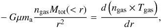 (3)where
G is the universal gravitational constant,
ma is the atomic mass unit and μ = 0.61
is the mean molecular weight in atomic mass unit. To solve this differential equation,
we need to define a boundary condition that is here fixed to the value of the pressure
measured in the outermost point of the gas density profile,
Pout = Pgas(Rsp) = ngas(Rsp) × Tgas(Rsp),
where Tgas(Rsp) is estimated
by linear extrapolation in the logarithmic space, if required. The systematic
uncertainties introduced by this assumption on Pout are
discussed in the next section. Note that by applying Method 1 the
errors on the gas density do not propagate into the estimates of the parameters of the
mass profile and are used both to define the range of the accepted values of
Pout and to evaluate the uncertainties on the gas mass
profiles. The allowed range at 1σ of the two interesting parameters,
rs and c200, is defined from
the minimum and the maximum of the values that permit
(3)where
G is the universal gravitational constant,
ma is the atomic mass unit and μ = 0.61
is the mean molecular weight in atomic mass unit. To solve this differential equation,
we need to define a boundary condition that is here fixed to the value of the pressure
measured in the outermost point of the gas density profile,
Pout = Pgas(Rsp) = ngas(Rsp) × Tgas(Rsp),
where Tgas(Rsp) is estimated
by linear extrapolation in the logarithmic space, if required. The systematic
uncertainties introduced by this assumption on Pout are
discussed in the next section. Note that by applying Method 1 the
errors on the gas density do not propagate into the estimates of the parameters of the
mass profile and are used both to define the range of the accepted values of
Pout and to evaluate the uncertainties on the gas mass
profiles. The allowed range at 1σ of the two interesting parameters,
rs and c200, is defined from
the minimum and the maximum of the values that permit  to be lower or equal to
min
to be lower or equal to
min . The average error on the mass is then
the mean of the upper and lower limit obtained at each radius from the allowed ranges
at 1σ of rs and
c200. Only for the purpose of estimating the profile of
Mgas( < r), and
eventually to provide the extrapolated values, the deprojected gas density profile is
fitted with the generic functional form described in Ettori et al. (2009) and adapted from the one described in
Vikhlinin et al. (2006),
ngas = ngas,0(r/rc,0) − α0 × (1 + (r/rc,0)2) − 1.5α1 + α0/2 × (1 + (r/rc,1)α2) − α3/α2.
. The average error on the mass is then
the mean of the upper and lower limit obtained at each radius from the allowed ranges
at 1σ of rs and
c200. Only for the purpose of estimating the profile of
Mgas( < r), and
eventually to provide the extrapolated values, the deprojected gas density profile is
fitted with the generic functional form described in Ettori et al. (2009) and adapted from the one described in
Vikhlinin et al. (2006),
ngas = ngas,0(r/rc,0) − α0 × (1 + (r/rc,0)2) − 1.5α1 + α0/2 × (1 + (r/rc,1)α2) − α3/α2.
(Method 2) The second method follows the approach described in Humphrey et al. (2006) and Gastaldello et al. (2007) where further details of this technique (in particular in Appendix B of Gastaldello et al. 2007) are provided. We assume parametrizations for the gas density and mass profiles to calculate the gas temperature assuming hydrostatic equilibrium,
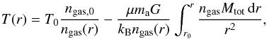 (4)where
ngas is the gas density,
ngas,0 and
T0 are density and temperature at some “reference”
radius r0 and kB is
Boltzmann’s constant. The ngas and
T(r) profiles are fitted simultaneously to the
data to constrain the parameters of the gas density and mass models. The parameters of
the mass model are obtained from fitting the gas density and temperature data and
goodness-of-fit for any mass model can be assessed directly from the residuals of the
fit. The quality of the data, in particular of the temperature profile, motivated the
use of this approach rather than the default approach of parametrizing the temperature
and mass profiles to calculate the gas density used in Gastaldello et al. (2007). We projected the parametrized models of the
three-dimensional quantities,
(4)where
ngas is the gas density,
ngas,0 and
T0 are density and temperature at some “reference”
radius r0 and kB is
Boltzmann’s constant. The ngas and
T(r) profiles are fitted simultaneously to the
data to constrain the parameters of the gas density and mass models. The parameters of
the mass model are obtained from fitting the gas density and temperature data and
goodness-of-fit for any mass model can be assessed directly from the residuals of the
fit. The quality of the data, in particular of the temperature profile, motivated the
use of this approach rather than the default approach of parametrizing the temperature
and mass profiles to calculate the gas density used in Gastaldello et al. (2007). We projected the parametrized models of the
three-dimensional quantities,  and T,
and fitted these projected emission-weighted models to the results obtained from our
analysis of the data projected on the sky. With respect to the paper cited above, the
XSPEC normalization have been derived converting the XMM surface brightness in the
0.7 − 1.2 keV band using the effective area and observed projected temperature and
metallicity obtained in the wider radial bins used for spectral extraction. The models
have been integrated over each radial bin (rather than only evaluating at a single
point within the bin) to provide a consistent comparison. We considered an NFW profile
of Eq. (1) for fitting the total mass
and two models for fitting the gas density profile: the β model
(Cavaliere & Fusco-Femiano 1978) a
double β model in which a common value of beta is assumed, and a
cusped β model (Pratt & Arnaud 2002; Lewis et al. 2003).
The last two models have been introduced to account for the sharply peaked surface
brightness in the centers of relaxed X-ray systems and they provide the necessary
flexibility to parametrize adequately the shape of the gas density profiles of the
objects in our sample when the traditional β model fails in fitting
the data.
and T,
and fitted these projected emission-weighted models to the results obtained from our
analysis of the data projected on the sky. With respect to the paper cited above, the
XSPEC normalization have been derived converting the XMM surface brightness in the
0.7 − 1.2 keV band using the effective area and observed projected temperature and
metallicity obtained in the wider radial bins used for spectral extraction. The models
have been integrated over each radial bin (rather than only evaluating at a single
point within the bin) to provide a consistent comparison. We considered an NFW profile
of Eq. (1) for fitting the total mass
and two models for fitting the gas density profile: the β model
(Cavaliere & Fusco-Femiano 1978) a
double β model in which a common value of beta is assumed, and a
cusped β model (Pratt & Arnaud 2002; Lewis et al. 2003).
The last two models have been introduced to account for the sharply peaked surface
brightness in the centers of relaxed X-ray systems and they provide the necessary
flexibility to parametrize adequately the shape of the gas density profiles of the
objects in our sample when the traditional β model fails in fitting
the data.
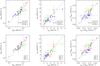 |
Fig. 5 Estimates of M200 (left), c200 (center) and fgas(<R500) (right) with the two methods. (Upper panels) The color code indicates the objects at z < 0.15 (blue), in the range 0.15 < z < 0.25 (green) and at z > 0.25 (red). (Lower panels) Distribution of Low (LEC), Medium (MEC), High (HEC) Entropy Core systems. |
The best-fit values obtained for an assumed NFW dark matter mass profiles are quoted in Table 2. In Table 3, we present our estimates of R200, R500 and the gas mass fraction fgas = Mgas/Mtot, that is hereafter considered within R500 to avoid a problematic extrapolation of the data up to R200. In Fig. 3, we show the relative errors provided from the two methods on the estimates of c200 and M200. The distribution of the statistical uncertainties is comparable, with median values of 15–20% on both c200 and M200 with Method 1 and Method 2. Also the distributions of the measurements of c200 and M200 are very similar, with 1st–3rd quartile range of 2.70 − 5.29 and 4.7 − 11.1 × 10¹⁴ M⊙ with Method 1 and 3.17 − 5.09 and 4.3 − 9.1 × 10¹⁴ M⊙ with Method 2.
Moreover, the two methods show a good agreement between the two estimates of the gas mass fraction fgas(<R500), as shown in Fig. 5. We measure a median (1st, 3rd quartile) of 0.131(0.106,0.147), and a median relative error of 12%, with Method 1 and 0.124(0.108,0.155), and a relative error of 10%, with Method 2.
As shown in the last two panels of Fig. 3, we note that the large majority of our data is able to define a scale radius rs well within the radial range investigated in the spectral and spatial analysis, allowing a quite robust constraints of the fitted parameters.
To rely on the best estimates of the concentration and mass, we define in the following analysis a further subsample by collecting the clusters that satisfy the criterion that the upper value at 1σ of the scale radius, as estimated from the 2 methods, is lower than the upper limit of the spatial extension of the detected X-ray emission, i.e. (rs + ϵrs) < Rsp. Imposing this condition, we select the 26 clusters where a more robust (i.e. with well defined and constrained free parameters) mass reconstruction is achievable.
Median deviations measured in the distribution of c200, MDM and fgas.
4. Systematics in the measurements of c200, M200 and fgas
The derived quantities c200, M200 and fgas(<R500) are measured with a relative statistical error of about 20, 15 and 10%, respectively (see Sect. 3 and Figs. 3 and 5). Here, we investigate the main uncertainties affecting our techniques that will be treated as systematic effects in the following analysis.
We consider two main sources of systematic errors: (i) the analysis of our dataset, both for what concerns the estimates of the gas temperature and the reconstructed gas density profile; (ii) the limitations and assumptions in the techniques adopted for the mass reconstruction.
In Table 4, we summarize our findings tabulated as relative median difference with respect to the estimates obtained with Method 1. Overall, we register systematic uncertainties of (−5, + 1)% on c200, (−4, + 3)% on M200 and (−1, + 4)% on fgas(<R500), where these ranges represent the minimum and maximum estimated in the dataset investigated and quoted in Table 4.
4.1. Systematics from the spectral analysis
The ICM properties of the present dataset have been studied through spatially resolved spectroscopic measurements of the gas temperature profile and deprojected, PSF-corrected surface brightness profile as accessible to XMM-Newton (see Sect. 2).
To assess the systematics propagated through the temperature measurements, we present the results obtained with M2 only, i.e. before any correction introduced from the harder spectra observed with M1 (see Sect. 2.1). Overall, the systematics are in the order of a few per cent, with the largest offset of about 4 per cent on the concentration and mass measurements at R500 and beyond.
When the deprojected spectral values of the gas temperature, instead of the projected ones, are compared with the predictions from the model, we measure differences below 5% (see dataset labelled “T3D”).
On the gas density profile, we investigate the role played from the use of a functional form instead of the values obtained directly from deprojection. To this purpose, we use a revised form of the one introduced from Vikhlinin et al. (2006) to fit the gas density profile and, then, we adopt it as representative of the gas density profile to be put in hydrostatic equilibrium with the gravitational potential in Eq. (3). The measurements obtained are labelled “fit ngas” and show discrepancies in the order of 1 per cent or less.
4.2. Systematics from the mass reconstruction methods
With the intention to assess the the bias affecting the reconstructed mass values, we make use of the gas temperature and density profiles through two independent techniques (labelled Method 1 and Method 2), as described in Sect. 3. With respect to Method 1, Method 2 provides differences on MDM that are lower than 10 per cent, increasing from about 1 per cent at R200 up to 7 per cent at R2500 (see Table 4). The bias on fgas remains stable around 3–4 per cent, suggesting that some systematics affect also the estimate of Mgas. This is due to the application of two different functional forms in Method 1 and Method 2 over a radial range that extends beyond the observational limit (see, e.g., Fig. 3).
The mass reconstruction of Method 1 depends upon the boundary condition on the gas pressure profile. In particular, to solve the differential Eq. (3), an outer value on the pressure is fixed to the product of the observed estimate of the gas density profile at the outermost radius and an extrapolated measurement of the gas temperature. Using a grid of values for the pressure obtained from the best-fit results of the gas density and temperature profiles, we evaluate a systematic bias on the mass of about 3 per cent, on the gas mass fraction of 1 per cent, and on c200 of about 1 per cent (see dataset labelled “Pout”).
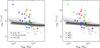 |
Fig. 6 Data in the plane (c200,M200) used to constrain the cosmological parameters (Ωm,σ8). The dotted lines show the predicted relations from Eke et al. (2001) for a given ΛCDM cosmological model at z = 0 (from top to bottom: σ8 = 0.9 and σ8 = 0.7). The shaded regions show the predictions in the redshift range 0.1 − 0.3 for an assumed cosmological model in agreement with WMAP-1, 5 and 3 years (from the top to the bottom, respectively) from Bullock et al. (2001; after Macciò et al. 2008). The dashed lines indicate the best-fit range at 1σ obtained for relaxed halos in a WMAP-5 years cosmology from Duffy et al. (2008; thin lines: z = 0.1, thick lines: z = 0.3). Color codes and symbols as in Fig. 5. |
5. The c200 − M200 relation
In this section, we investigate the c200 − M200 relation. We note that our sample has not been selected to be representative of the cluster population in the given redshift range and, in the mean time, does not include only relaxed systems. Therefore, the results here presented on the c200 − M200 relation have to be just considered for a qualitative comparison with the predictions from numerical simulations and to assess differences or similitude with previous work on this topic.
As we show in Fig. 6 using the measurements obtained
with Method 1, the median relation between concentration and total masses
for CDM halos as function of redshift is represented well from the analytic algorithms, as
in N97, E01 and B01. These models relate the halo properties to the physical mechanism of
halo formation. Considering the weak dependence of the halo concentrations on the mass and
redshift, Dolag et al. (2004) introduced a
two-parameter functional form,
c = c0MB/(1 + z).
We consider this relation in its logarithmic form and fit linearly to our data the
expression: 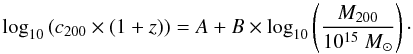 (5)A minimum in the
χ2 distribution is looked for by taking into account the
errors on both the coordinates (we use the routine FITEXY in IDL). The
errors are assumed to be Gaussian in the logarithmic space, although they are properly
measured as Gaussian in the linear space.
(5)A minimum in the
χ2 distribution is looked for by taking into account the
errors on both the coordinates (we use the routine FITEXY in IDL). The
errors are assumed to be Gaussian in the logarithmic space, although they are properly
measured as Gaussian in the linear space.
We also express our results in term of the concentration c15
expected for a dark matter halo of  and equal to
10A once the parameters in Eq. (5) are used. We convert to
c15 even the results from literature obtained, for instance,
at different overdensity, as described in the Appendix.
and equal to
10A once the parameters in Eq. (5) are used. We convert to
c15 even the results from literature obtained, for instance,
at different overdensity, as described in the Appendix.
Best-fit values of the c200 − M200 relation.
We measure A ≈ 0.6 and B systematically lower than −0.1, with the best-fit results obtained through Method 1 that prefer, with respect to Method 2, a relation with slightly higher normalization (by ~10 per cent) and flatter (by 10 − 30 per cent) distribution in mass. In both cases, a total scatter of σlog 10c ≈ 0.13 is measured both in the whole sample of 44 objects, where the statistical scatter related to the observed uncertainties is still dominant, and in the subsample of 26 selected clusters.
When a slope B = − 0.1 is assumed, as measured in numerical simulations over one order of magnitude in mass almost independently from the underlying cosmological model (see e.g. Dolag et al. 2004; Macciò et al. 2008), the measured normalizations of the c200 − M200 relation fall into the range of the estimated values for samples of simulated clusters (see Table 5).
All the values of normalization and slope are confirmed, within the estimated errors, with both the BCES bisector method (as described in Akritas & Bershady 1996 and implemented in the routines made available from Bershady) and a Bayesian method that accounts for measurement errors in linear regression, as implemented in the IDL routine LINMIX_ERR by Kelly (see Kelly 2007). As we quote in Table 5, with these linear regression methods (and after 106 bootstrap resampling of the data in BCES), we measure a typical error that is larger by a factor 2 − 3 in normalization and up to 6 in the slope than the corresponding values obtained through the covariance matrix of the FITEXY method.
These values compare well with the measurements obtained from numerical simulations of DM-only galaxy clusters, although these simulations sample, on average, mass ranges lower than the ones investigated here. Recent work from Shaw et al. (2006) and Macciò et al. (2008) summarize the findings. The slope of the relation, as previously obtained from B01 and D04, lies in the range ( − 0.160, − 0.083), with a preferred value of about − 0.1. The normalizations for low-density Universe with a relatively higher σ8, as from WMAP-1, are more in agreement with the observed constraints on, e.g., c15. For instance, M08 find c15 = 4.18,3.41,3.56 for relaxed objects in a background cosmology that matches WMAP-1, 3 and 5 year data, respectively1. Shaw et al. (2006) measure c15 = 4.64 using a flat Universe with Ωm = 0.3 and σ8 = 0.95. D04 for a ΛCDM with σ8 = 0.9 require c15 = 4.29. All these values show the sensitivity of the normalization to the assumed cosmology, that is further discussed in the section where constraints on the cosmological parameters (Ωm − σ8) will be obtained through the measured c − M relation. Neto et al. (2007) study the statistics of the halo concentrations at z = 0 in the Millennium Simulation (with an underlying cosmology of Ωm = 1 − ΩΛ = 0.25,σ8 = 0.9) and find that a power-law with B = − 0.10 and c15 = 4.33 fits fairly well the relation for relaxed objects, with an intrinsic logarithmic scatter for the most massive objects of 0.092 (see their Fig. 7).
We note, however, that, while the normalizations we measure for a fixed slope B = − 0.1 are well in agreement with the results from numerical simulations, a systematic lower value of the slope is measured, when it is left to vary. To test the robustness of this evidence, we have implemented Monte-Carlo runs using the best-fit central values estimated in N-body simulations (see Appendix B for details). With almost no dependence upon the input values from numerical simulations and using the FITEXY technique that provides the results with the most significant deviations from B ≈ −0.1, we measure in the 3 samples here considered (i.e. all 44 objects, the selected 26 objects, and the only 11 LEC objects) a probability of about 0.5 (1), 20 (42) and 26 (46) per cent, respectively, to obtain a slope lower than the measured 1(3)σ upper limit. These result confirm that the systematic uncertainties present in the measurements of the concentration and dark mass within R200 are still affecting the sample of 44 objects, whereas they are significantly reduced in the selected subsamples.
Our best-fit results are in good agreement also with previous constraints obtained from X-ray measurements in the same cosmology. Pointecouteau et al. (2005) measure c15 ≈ 4.5 and B = −0.04 ± 0.03 in a sample of ten nearby (z < 0.15) and relaxed objects observed with XMM-Newton in the temperature range 2 − 9 keV. Zhang et al. (2006) measure a steeper slope of − 1.5 ± 0.2, probably affected from few outliers, in the REFLEX-DXL sample of 13 X-ray luminous and distant (z ~ 0.3) clusters observed with XMM-Newton, that, they claim, are however not well reproduced from a NFW profile. Voigt & Fabian (2006) show a good agreement with B01 results and B ≈ −0.2 for their estimates of 12 mass profiles of X-ray luminous objects observed with Chandra in the redshift range 0.02 − 0.45. A good match with the results in D04, and within the scatter found in simulations, is obtained with 13 low-redshift relaxed systems with Tgas in the range 0.7 − 9 keV as measured with Chandra in Vikhlinin et al. (2006). Schmidt & Allen (2007), using Chandra observations of 34 massive relaxed galaxy clusters, measure B = − 0.45 ± 0.12 (95% c.l.), significantly steeper than the value predicted from CDM simulations. Leaving free the redshift dependence that they estimate to be consistent with the (1 + z)-1 expected evolution, they measure a normalization c15 ≈ 5.4 ± 0.6 (95% c.l.), definitely higher than our best-fit parameter. Buote et al. (2007) fit the c − M relation from 39 systems in the mass range 0.06−20 × 1014 M⊙ selected from Chandra and XMM-Newton archives to be relaxed. Analysing the tabulated values of the 20 galaxy clusters with M200 > 1014 M⊙, that include the most massive systems from the XMM-Newton study of Pointecouteau et al. (2005) and the Chandra analysis in Vikhlinin et al. (2006), we measure B = − 0.08 ± 0.05 and c15 ≈ 5.16 ± 0.36.
Overall, we conclude however that the slope of the c − M relation cannot be reliably determined from the fitting over a narrow mass range as the one considered in the present work and that, once the slope is fixed to the expected value of B = − 0.1, the normalization, with estimates of c15 in the range 3.8 − 4.6, agrees with results of previous observations and simulations for a calculations in a low density Universe.
5.1. The subsample of low-entropy-core objects
Following Leccardi et al. (2010), we have employed the pseudo-entropy ratio (σ ≡ (TIN/TOUT) × (EMIN/EMOUT) − 1/3, where IN and OUT define regions within ≈ 0.05 R180 and encircled in the annulus with bounding radii 0.05–0.20 R180, respectively, and T and EM are the cluster temperature and emission measure) to classify our sample of 44 galaxy clusters accordingly to their core properties. We identify 17 high-entropy-core (HEC), 11 medium-entropy-core (MEC) and 16 low-entropy-core (LEC; see Table 1) systems. While the MEC and HEC objects are progressively more disturbed (about 85 per cent of the merging clusters are HEC) and with a core that presents less evidence in the literature of a temperature decrement and a peaked surface brightness profile (intermediate, ICC, and no cool core, NCC, systems), the LEC objects represent the prototype of a relaxed cluster with a well defined cool core (CC in Table 1) at low entropy (see also Cavagnolo et al. 2009). These systems are predicted from numerical simulations to have higher concentrations for given mass, by about 10 per cent, and lower scatter, by about 15–20 per cent, in the c − M relation (e.g. M08, Duffy et al. 2008).
Out of 16, eleven LEC objects are selected under the condition that their scale radius is within the radial coverage of our data. We measure their c − M relation to have slightly lower normalization (A ≈ 0.5 − 0.6, c15 ≈ 3.2−3.7) and flatter distribution (B = −0.4 ± 0.2) than the one observed in the selected subsample of 26 objects, with a dispersion around the logarithmic value of the concentration of 0.08, that is about 40 per cent lower than the similar value observed in the latter sample. This is consistent in a scenario where disturbed systems have an estimated concentration through the hydrostatic equilibrium equation that is biased higher (and with larger scatter) than in relaxed objects up to a factor of 2 due to the action of the ICM motions (mainly the rotational term in the inner regions and the random gas term above R500), as discussed in Lau et al. (2009; see also Fang et al. 2009; Meneghetti et al. 2010) for galaxy clusters extracted from high-resolution Eulerian cosmological simulations.
6. Cosmological constraints from the measurements of c200,M200, and fgas
N-body simulations have provided theoretical fitting functions that are able to reproduce the distribution of the concentration parameter of the NFW density profile as function of halo mass and redshift (e.g. NFW, E01, B01, N07). Basically, all these semi-empirical prescriptions provide the expected values of the concentration parameter for a given set of cosmological parameters (essentially, the cosmic matter density, Ωm, and the normalization of the power spectrum on clusters scale, σ8) for a given mass (the estimated cluster dark mass, M200, in our case) at the measured redshift of the analyzed object. They assume that the concentration reflects the background density of the Universe at the formation time of a given halo. The cosmological model influences the concentration and virial mass because of the cosmic background density and the evolution of structure formation. For instance, the NFW model uses two free parameters, (f,C), to define the collapse redshift at which half of the final mass M is contained in progenitors of mass ≥ fM, with C representing the ratio between the characteristic overdensity and the mean density of the Universe at the collapse redshift. We use (f,C) = (0.1,3000).
B01 assume, instead, an alternative model to improve the agreement between the predicted redshift dependence of the concentrations and the results of the numerical simulations by using two free parameters, F and K, where F is still a fixed fraction (0.01 in our study) of a halo mass at given redshift and K indicates the concentration of the halo at the collapse redshift. K has to be calibrated with numerical simulations and is fixed here to be equal to 4 (see also Buote et al. 2007, for a detailed discussion on the role played from the parameters F and K on the prediction of the concentrations as function of the background cosmology and halo masses). M08 have revised this model by assuming that the characteristic density of the halo, that in B01 scales as (1 + z)3, is independent of redshift. This correction propagates into the growth factor of the concentration parameter that becomes shallower with respect to the mass dependence at masses higher than 1013 h-1 M⊙, permitting larger concentrations at the high-mass end than the original B01 formulation.
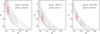 |
Fig. 7 Cosmological constraints in the
(Ωm,σ8) plane obtained from
Eqs. (6) and (7) by using predictions from the model by
Eke et al. (2001). The confidence contours at
1,2,3σ on 2 parameters (solid
contours) are displayed. The combined likelihood with the probability distribution
provided from the cluster gas mass fraction method is shown in red. The dashed green
line indicates the power-law fit |
Cosmological constraints on σ8 and Ωm.
The prescription in E01 defines with the only parameter
Cσ (equal to 28, in our analysis, as
suggested in their original work) the collapse redshift zc
through the relation  , where
D(z) is the linear growth factor,
σeff is the effective amplitude of the linear power spectrum
at z = 0 and Ms is the total mass within the
radius at which the circular velocity of an NFW halo reaches its maximum and that is equal
to 2.17 times the scale radius, rs.
, where
D(z) is the linear growth factor,
σeff is the effective amplitude of the linear power spectrum
at z = 0 and Ms is the total mass within the
radius at which the circular velocity of an NFW halo reaches its maximum and that is equal
to 2.17 times the scale radius, rs.
As tested in high-resolution numerical simulations (see, e.g., N07, M08, Duffy et al. 2008), these 3 formulations provide different predictions over different mass range and redshift: for massive systems a z < 1, as the ones under investigation in the present analysis, the original B01 tends to underestimate the concentration at fixed halo mass; its revised version after M08 partially compensate for this difference but still shows some tension with numerically simulated objects (see, e.g., Fig. 5 in M08); NFW overestimates the concentration, whereas E01 provide good estimates (see, e.g. Fig. 2 in Duffy et al. 2008) also considering its simpler and more robust formulation, being dependent upon a single parameter that does not need an independent calibration from simulations evolved with a given background cosmology (note, indeed, that as pointed out in M08, both NFW and B01 models have normalizations that, ideally, have to be determined empirically for each assumed cosmology with a dedicated numerical simulation).
Hereafter, we consider E01 as the model of reference and use the other prescriptions as estimate of the systematics affecting our constraints.
In particular, to constrain the cosmological parameters of interest, σ8 and Ωm, we calculate first the concentration c200,ijk = c200(Mi,Ωm,j,σ8,k) predicted from the model investigated at each cluster redshift for a given grid of values in mass, Mi, cosmic density parameter, Ωm,j, and power spectrum normalization, σ8,k.
Then, we proceed with the following analysis:
- 1.
a new mass M200,j and concentration c200,j are estimated from the X-ray data for given Ωm,j;
- 2.
we perform a linear interpolation on the theoretical prediction of c200,ijk to associate a concentration ĉ200,jk to the new mass M200,j for given Ωm,j and σ8,k;
- 3.
we evaluate the merit function

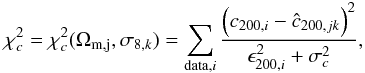 (6)where
ϵ200,i is the 1σ
uncertainty related to the measured
c200,i and
σc is the scatter intrinsic to the
mean predicted value ĉ200,jk as evaluated
in Neto et al. (2007; see their Fig. 7 and
relative discussion). They estimate in the mass bin
1014.25−1014.75 h-1 M⊙
a logarithmic mean value of the concentration parameter of 0.663, with a dispersion of
0.092, corresponding to a relative uncertainty of 0.139. We take into account these
estimates by associating to the expectation of
ĉ200,jk a scatter equals to
(6)where
ϵ200,i is the 1σ
uncertainty related to the measured
c200,i and
σc is the scatter intrinsic to the
mean predicted value ĉ200,jk as evaluated
in Neto et al. (2007; see their Fig. 7 and
relative discussion). They estimate in the mass bin
1014.25−1014.75 h-1 M⊙
a logarithmic mean value of the concentration parameter of 0.663, with a dispersion of
0.092, corresponding to a relative uncertainty of 0.139. We take into account these
estimates by associating to the expectation of
ĉ200,jk a scatter equals to
 , where
ϵc = 0.139 × log ĉ200,jk;
, where
ϵc = 0.139 × log ĉ200,jk;
- 4.
a minimum in the
distribution,
 , is evaluated and the
regions encompassing
, is evaluated and the
regions encompassing  are estimated to
constrain the best-fit values and the
1,2,3σ intervals in the
(Ωm,σ8) plane shown in
Fig. 7. To represent the observed degeneracy in
the σ8 − Ωm plane, we quote in Table 6 (and show with a dashed line in Fig. 7) the best-fit values of the power-law fit
are estimated to
constrain the best-fit values and the
1,2,3σ intervals in the
(Ωm,σ8) plane shown in
Fig. 7. To represent the observed degeneracy in
the σ8 − Ωm plane, we quote in Table 6 (and show with a dashed line in Fig. 7) the best-fit values of the power-law fit
 ,
obtained by fitting this function on a grid of values estimated, at each assigned
Ωm, the best-fit result, and associated 1σ error, of
σ8.
,
obtained by fitting this function on a grid of values estimated, at each assigned
Ωm, the best-fit result, and associated 1σ error, of
σ8. - 5.
A further constraint on the Ωm parameter that allows us to break the degeneracy in the σ8 − Ωm plane (as highlighted from the banana-shape of the likelihood contours plotted in Fig. 7) is provided from the gas mass fraction distribution. We use our estimates of fgas(<R500) = f500 from Method 1 quoted in Table 3. We follow the procedure described in Ettori et al. (2009) and assume: (i)
 and
H0 = 70.1 ± 1.3 from the best-fit results of the joint
analysis in Komatsu et al. (2008); (ii) a depletion parameter at
R500b500 = 0.874 ± 0.023;
(iii) a contribution of cold baryons to the total budget
fcold = 0.18( ± 0.05)fgas.
All the quoted errors are at 1σ level. Then, we look for a minimum in
the function
and
H0 = 70.1 ± 1.3 from the best-fit results of the joint
analysis in Komatsu et al. (2008); (ii) a depletion parameter at
R500b500 = 0.874 ± 0.023;
(iii) a contribution of cold baryons to the total budget
fcold = 0.18( ± 0.05)fgas.
All the quoted errors are at 1σ level. Then, we look for a minimum in
the function 
![Mathematical equation: \begin{equation} \chi_{f}^2 = \sum_{{\rm data}, i} \frac{\left[ f_{500, i} (1+ f_{\rm cold})/b_{500} - \hat{f}_{{\rm bar}, j} \right]^2} {\epsilon_{f, i}^2}, \label{eq:chi2f} \end{equation}](/articles/aa/full_html/2010/16/aa15271-10/aa15271-10-eq1160.png) (7)where
(7)where
 and
ϵf,i is given from the sum in
quadrature of all the statistical errors, namely, on
f500,fcold,H0,b500
and Ωb.
and
ϵf,i is given from the sum in
quadrature of all the statistical errors, namely, on
f500,fcold,H0,b500
and Ωb. - 6.
We combine the two χ2 distribution,
 , and plot in Fig. 7 the constraints obtained from both
only and
, and plot in Fig. 7 the constraints obtained from both
only and
 , quoting the best-fit
results in Table 6.
, quoting the best-fit
results in Table 6.
- 7.
The effect of the systematic uncertainties, assumed to be normally distributed, is also considered by propagating them in quadrature to the measurements of c200 and f500, as obtained from the analysis summarized in Table 4. The constraints obtained after this further correction are indicated with label “ + syst” in Table 6.
. As expected from the
properties of the prescriptions, E01 provides constraints on σ8,
for given Ωm, that lie between the other two, with
γ = 0.60 ± 0.04 and Γ = 0.44 ± 0.02 (at 2σ level;
statistical only). We break the degeneracy of the best-fit values in the
(σ8,Ωm) plane by assuming that the
cluster baryon fraction represents the cosmic value well. We obtain that
σ8 = 1.0 ± 0.2 and Ωm = 0.27 ± 0.01 (at
2σ level). When the subsample of 11 LEC clusters, that are expected to be
more relaxed and with a well-formed central cooling core, is considered, we measure
γ = 0.55 ± 0.05, Γ = 0.40 ± 0.02
σ8 = 0.85 ± 0.16 and Ωm = 0.27 ± 0.01 (at
2σ level).
We confirm that, assumed correct the ones measured with E01, NFW tends to overestimate the predicted concentrations and, therefore, requires lower normalization σ8 of the power spectrum, whereas B01+M08 compensate with larger values of σ8 the underestimate of c200 with respect to E01.
We assess the systematics affecting our results by comparing the cosmological constraints obtained by assuming (i) different algorithms to relate the cosmological models to the derived c − M relation; (ii) biases both in the concentration parameter (bc = 0.9), from the evidence in numerical simulations that relaxed halos have an higher concentration by about 10 per cent (e.g. Duffy et al. 2008), and in the dark matter (bM = 1.1) measurements from the evidence provided from hydrodynamial simulations that the hydrostatic equilibrium might underestimate the true mass by 5–20 per cent (e.g. see recent work in Meneghetti et al. 2010). As expected, lower concentrations and higher masses push the best-fit values to lower normalizations of the power spectrum at fixed Ωm, with an offset of about 10 per cent with bc = 0.9 and of few per cent bM = 1.1 and Mtot.
7. Summary and conclusions
We present the reconstruction of the dark and gas mass from the XMM-Newton observations of 44 massive X-ray luminous galaxy clusters in the redshift range 0.1 − 0.3. We estimate a dark (Mtot − Mgas) mass within R200 in the range (1st and 3rd quartile) 4 − 10 × 1014 M⊙, with a concentration c200 between 2.7 and 5.3, and a gas mass fraction within R500 between 0.11 and 0.16.
By applying the equation of the hydrostatic equilibrium to the spatially resolved estimates of the spectral temperature and normalization, we recover the underlying gravitational potential of the dark matter halo, assumed to be well described from a NFW functional form, with two independent techniques.
Our dataset is able to resolve the temperature profiles up to about 0.6 − 0.8R500 and the gas density profile, obtained from the geometrical deprojection of the PSF-deconvolved surface brightness, up to a median radius of 0.9R500. Beyond this radial end, our estimates are the results of an extrapolation obtained by imposing a NFW profile for the total mass and different functional forms for Mgas.
We estimate, with a relative statistical uncertainty of 15 − 25%, the concentration
c200 and the mass M200 of the dark
matter (i.e. total-gas mass) halo. We constrain the
c200 − M200 relation to have a
normalization 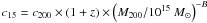 of about 2.9 − 4.2 and a
slope B between − 0.3 and − 0.7 (depending on the methods used to recover
the cluster parameters and to fit the linear correlation in the logarithmic space), with a
relative error of about 5% and 15%, respectively. Once the slope is fixed to the expected
value of B = −0.1, the normalization, with estimates of
c15 in the range 3.8 − 4.6, agrees with results of previous
observations and simulations for calculations done assuming a low density Universe. We
conclude thus that the slope of the
c200 − M200 relation cannot be
reliably determined from the fitting over a narrow mass range as the one considered in the
present work, altough the steeper values measured are not significantly in tension with the
results for simulated halos when the subsamples of the most robust estimates are considered
(see Sect. 5 and Appendix B). We measure a total scatter in the logarithmic space of about
0.15 at fixed mass. This value decreases to 0.08 when the subsample of LEC clusters is
considered, where a slightly lower normalization and flatter distribution is measured. This
is consistent in a scenario where disturbed systems have an estimated concentration through
the hydrostatic equilibrium equation that is biased higher (and with larger scatter) than in
relaxed objects up to a factor of 2 due to the action of the ICM motions (see e.g. Lau
et al. 2009).
of about 2.9 − 4.2 and a
slope B between − 0.3 and − 0.7 (depending on the methods used to recover
the cluster parameters and to fit the linear correlation in the logarithmic space), with a
relative error of about 5% and 15%, respectively. Once the slope is fixed to the expected
value of B = −0.1, the normalization, with estimates of
c15 in the range 3.8 − 4.6, agrees with results of previous
observations and simulations for calculations done assuming a low density Universe. We
conclude thus that the slope of the
c200 − M200 relation cannot be
reliably determined from the fitting over a narrow mass range as the one considered in the
present work, altough the steeper values measured are not significantly in tension with the
results for simulated halos when the subsamples of the most robust estimates are considered
(see Sect. 5 and Appendix B). We measure a total scatter in the logarithmic space of about
0.15 at fixed mass. This value decreases to 0.08 when the subsample of LEC clusters is
considered, where a slightly lower normalization and flatter distribution is measured. This
is consistent in a scenario where disturbed systems have an estimated concentration through
the hydrostatic equilibrium equation that is biased higher (and with larger scatter) than in
relaxed objects up to a factor of 2 due to the action of the ICM motions (see e.g. Lau
et al. 2009).
We put constraints on the cosmological parameters
(σ8,Ωm) by using the measurements
of c200 and M200 and by comparing
the estimated values with the predictions tuned from numerical simulations of CDM universes.
In doing that, we propagate the statistical errors (with a relative value of about 15 − 25%
at 1σ level) and consider the systematic uncertainties present both in the
simulated datasets (~20%) and in our measurements (~10%; see Table 4). To represent the observed degeneracy, we constrain
the parameters of the power-law fit and obtain
γ = 0.60 ± 0.03 and Γ = 0.45 ± 0.02 (at 2σ level) when
the E01 formalism is adopted. Different formalisms (like the ones in B01, revised after M08,
and NFW) induce variations in the best-fit parameters in the order of 20 per cent. A further
variation of about 10 per cent occurs if a bias of the order of 10 per cent is considered on
the estimates of c200 and M200.
We break the degeneracy of the best-fit values in the (σ8,Ωm) plane by assuming that the cluster baryon fraction represents the cosmic value well. We obtain that σ8 = 1.0 ± 0.2 and Ωm = 0.26 ± 0.01 (at 2σ level; statistical only).
When the subsample of 11 LEC clusters, that are expected to be more relaxed and with a well-formed central cooling core, is considered, we measure γ = 0.56 ± 0.04, Γ = 0.39 ± 0.02 σ8 = 0.83 ± 0.1 and Ωm = 0.26 ± 0.02 (at 2σ level).
All these estimates agree well with similar constraints obtained for an assumed low-density Universe in Buote et al. (2007; 0.76 < σ8 < 1.07 at 99% confidence for a ΛCDM model with Ωm = 0.3) and with the results obtained by analysing the mass function of rich galaxy clusters (see, e.g., Wen et al. 2010 that summarizes recent results obtained by this cosmological tool), showing that the study of the distribution of the measurements in the c − MDM − fgas plane provides a valid technique already mature and competitive in the present era of precision cosmology.
However, we highlight the net dependence of our results on the models adopted to relate the properties of a DM halo to the background cosmology. In this context, we urge the N-body community to generate cosmological simulations over a large box to properly predict the expected concentration associated to the massive ( > 1014 M⊙) DM halos as function of σ8, Ωm and redshift. The detailed analysis of the outputs of these datasets will provide the needed calibration to make this technique more reliable and robust.
We refer to Appendix A for a detailed discussion of the conversions adopted.
Acknowledgments
The anonymous referee is thanked for suggestions that have improved the presentation of the work. We acknowledge the financial contribution from contracts ASI-INAF I/023/05/0 and I/088/06/0. This research has made use of the X-Rays Clusters Database (BAX) which is operated by the Laboratoire d’Astrophysique de Tarbes-Toulouse (LATT), under contract with the Centre National d’Etudes Spatiales (CNES).
References
- Akritas, M. G., & Bershady, M. A. 1996, ApJ, 470, 706 [NASA ADS] [CrossRef] [Google Scholar]
- Allen, S. W., Schmidt, R. W., & Fabian, A. C. 2001, MNRAS, 328, L37 [NASA ADS] [CrossRef] [Google Scholar]
- Andreon, S. 2010, MNRAS, 407, 263 [NASA ADS] [CrossRef] [Google Scholar]
- Arnaud, K. A. 1996, Astronomical Data Analysis Software and Systems V, ed. G. Jacoby, & J. Barnes, ASP Conf. Ser., 101, 17 [Google Scholar]
- Arnaud, M., Pointecouteau, E., & Pratt, G. W. 2005, A&A, 441, 893 [NASA ADS] [CrossRef] [EDP Sciences] [Google Scholar]
- Baldi, A., Ettori, S., Mazzotta, P., Tozzi, P., & Borgani, S. 2007, ApJ, 666, 835 [NASA ADS] [CrossRef] [Google Scholar]
- Bullock, J. S., Kolatt, T. S., Sigad, Y., et al. 2001, MNRAS, 321, 559 [Google Scholar]
- Buote, D. A. 2000, ApJ, 539, 172 [NASA ADS] [CrossRef] [Google Scholar]
- Buote, D. A., Gastaldello, F., Humphrey, P. J., et al. 2007, ApJ, 664, 123 [NASA ADS] [CrossRef] [Google Scholar]
- Cavaliere, A., & Fusco-Femiano, R. 1978, A&A, 70, 677 [NASA ADS] [Google Scholar]
- Cavagnolo, K. W., Donahue, M., Voit, G. M., & Sun, M. 2009, ApJS, 182, 12 [NASA ADS] [CrossRef] [Google Scholar]
- Comerford, J. M., & Natarajan, P. 2007, MNRAS, 379, 190 [NASA ADS] [CrossRef] [Google Scholar]
- Croston, J. H., Pratt, G. W., Böhringer, H., et al. 2008, A&A, 487, 431 [NASA ADS] [CrossRef] [EDP Sciences] [Google Scholar]
- Dickey, J. M., & Lockman, F. J. 1990, ARAA, 28, 215 [NASA ADS] [CrossRef] [Google Scholar]
- Dolag, K., Bartelmann, M., Perrotta, F., et al. 2004, A&A, 416, 853 [NASA ADS] [CrossRef] [EDP Sciences] [Google Scholar]
- Donnarumma, A., Ettori, S., Meneghetti, M., & Moscardini, L. 2009, MNRAS, 398, 438 [NASA ADS] [CrossRef] [Google Scholar]
- Donnarumma, A., Ettori, S., Meneghetti, M., et al. 2010, A&A, in press [arXiv:1002.1625] [Google Scholar]
- Duffy, A. R., Schaye, J., Kay, S. T., & Dal la Vecchia, C. 2008, MNRAS, 390, L64 [NASA ADS] [CrossRef] [Google Scholar]
- Eke, V. R., Navarro, J. F., & Steinmetz, M. 2001, ApJ, 554, 114 [NASA ADS] [CrossRef] [Google Scholar]
- Ettori, S., De Grandi, S., & Molendi, S. 2002, A&A, 391, 841 [NASA ADS] [CrossRef] [EDP Sciences] [Google Scholar]
- Ettori, S., Morandi, A., Tozzi, P., et al. 2009, A&A, 501, 61 [NASA ADS] [CrossRef] [EDP Sciences] [Google Scholar]
- Fabian, A. C., Hu, E. M., Cowie, L. L., & Grindlay, J. 1981, ApJ, 248, 47 [NASA ADS] [CrossRef] [Google Scholar]
- Fang, T., Humphrey, P., & Buote, D. 2009, ApJ, 691, 1648 [NASA ADS] [CrossRef] [Google Scholar]
- Finoguenov, A., Boehringer, H., & Zhang, Y.-Y. 2005, A&A, 442, 827 [NASA ADS] [CrossRef] [EDP Sciences] [Google Scholar]
- Gao, L., Navarro, J. F., Cole, S., et al. 2008, MNRAS, 387, 536 [NASA ADS] [CrossRef] [Google Scholar]
- Gastaldello, F., Buote, D. A, Humphrey, P. J., et al. 2007, ApJ, 669, 158 [NASA ADS] [CrossRef] [Google Scholar]
- Ghizzardi, S. 2001, In Flight Calibration of the PSF for the MOS1 and MOS2 Cameras, EPIC-MOS-TN-11 [Google Scholar]
- Govoni, F., Markevitch, M., Vikhlinin, A., et al. 2004, ApJ, 605, 695 [NASA ADS] [CrossRef] [Google Scholar]
- Humphrey, P. J., Buote, D. A, Gastaldello, F., et al. 2006, ApJ, 646, 899 [NASA ADS] [CrossRef] [Google Scholar]
- Kelly, B. C. 2007, ApJ, 665, 1489 [NASA ADS] [CrossRef] [Google Scholar]
- Kempner, J. C., Sarazin, C. L., & Markevitch, M. 2003, ApJ, 593, 291 [NASA ADS] [CrossRef] [Google Scholar]
- Kriss, G. A., Cioffi, D. F., & Canizares, C. R. 1983, ApJ, 272, 439 [NASA ADS] [CrossRef] [Google Scholar]
- Kuhlen, M., Strigari, L. E., Zentner, A. R., Bullock, J. S., & Primack, J. R. 2005, MNRAS, 357, 387 [NASA ADS] [CrossRef] [Google Scholar]
- Lau, E. T., Kravtsov, A. V., & Nagai, D. 2009, ApJ, 705, 1129 [NASA ADS] [CrossRef] [Google Scholar]
- Leccardi, A., & Molendi, S. 2008a, A&A, 486, 359 [NASA ADS] [CrossRef] [EDP Sciences] [Google Scholar]
- Leccardi, A., & Molendi, S. 2008b, A&A, 487, 461 [NASA ADS] [CrossRef] [EDP Sciences] [Google Scholar]
- Leccardi, A., Rossetti, M., & Molendi, S. 2010, A&A, 510, 82 [Google Scholar]
- Lewis, A. D., Buote, D. A., & Stocke, J. T. 2003, ApJ, 586, 135 [NASA ADS] [CrossRef] [Google Scholar]
- Lin, W. P., Jing, Y. P., Mao, S., Gao, L., & McCarthy, I. G. 2006, ApJ, 651, 636 [NASA ADS] [CrossRef] [Google Scholar]
- Macciò, A. V., Dutton, A. A., & van den Bosch, F. C. 2008, MNRAS, 391, 1940 [NASA ADS] [CrossRef] [Google Scholar]
- Mateos, S., Saxton, R. D., Read, A. M., & Sembay, S. 2009, A&A, 496, 879 [NASA ADS] [CrossRef] [EDP Sciences] [Google Scholar]
- Mazzotta, P., Rasia, E., Moscardini, L., & Tormen, G. 2004, MNRAS, 354, 10 [NASA ADS] [CrossRef] [Google Scholar]
- Meneghetti, M., Rasia, E., Merten, J., et al. 2010, A&A, 514, 93 [Google Scholar]
- Morandi, A., Ettori, S., & Moscardini, L. 2007, MNRAS, 379, 518 [NASA ADS] [CrossRef] [Google Scholar]
- McLaughlin, D. E. 1999, AJ, 117, 2398 [NASA ADS] [CrossRef] [Google Scholar]
- Navarro, J. F., Frenk, C. S., & White, S. D. M. 1997, ApJ, 490, 493 [NASA ADS] [CrossRef] [Google Scholar]
- Navarro, J. F., Hayashi, E., Power, C., et al. 2004, MNRAS, 349, 1039 [NASA ADS] [CrossRef] [Google Scholar]
- Neto, A. F., Gao, L., Bett, P., et al. 2007, MNRAS, 381, 1450 [NASA ADS] [CrossRef] [Google Scholar]
- Pointecouteau, E., Arnaud, M., & Pratt, G. W. 2005, A&A, 435, 1 [NASA ADS] [CrossRef] [EDP Sciences] [Google Scholar]
- Pratt, G. W., & Arnaud, M. 2002, A&A, 394, 375 [NASA ADS] [CrossRef] [EDP Sciences] [Google Scholar]
- Pratt, G. W., Böhringer, H., Croston, J. H., et al. 2007, A&A, 461, 71 [NASA ADS] [CrossRef] [EDP Sciences] [Google Scholar]
- Press, W. H., Teukolsky, S. A., Vetterling, S. A., & Flannery, B. P. 1992, Numerical Recipes in Fortran, 2nd edn., 660 [Google Scholar]
- Rasia, E., Ettori, S., Moscardini, L., et al. 2006, MNRAS, 369, 2013 [NASA ADS] [CrossRef] [Google Scholar]
- Sanderson, A. J. R., O’Sullivan, E., & Ponman, T. J. 2009, MNRAS, 395, 764 [NASA ADS] [CrossRef] [Google Scholar]
- Schmidt, R. W., & Allen, S. W. 2007, MNRAS, 379, 209 [NASA ADS] [CrossRef] [Google Scholar]
- Shaw, L. D., Weller, J., Ostriker, J. P., & Bode, P. 2006, ApJ, 646, 815 [NASA ADS] [CrossRef] [Google Scholar]
- Sivanandam, S., Zabludoff, A. I., Zaritsky, D., Gonzalez, A. H., & Kelson, D. D. 2009, ApJ, 691, 1787 [NASA ADS] [CrossRef] [Google Scholar]
- Snowden, S. L., Mushotzky, R. F., Kuntz, K. D., & Davis, D. S. 2008, A&A, 478, 615 [NASA ADS] [CrossRef] [EDP Sciences] [Google Scholar]
- Vikhlinin, A., Markevitch, M., Murray, S. S., et al. 2005, ApJ, 628, 655 [NASA ADS] [CrossRef] [Google Scholar]
- Vikhlinin, A., Kravtsov, A., Forman, W., et al. 2006, ApJ, 640, 691 [NASA ADS] [CrossRef] [Google Scholar]
- Voigt, L. M., & Fabian, A. C. 2006, MNRAS, 368, 518 [NASA ADS] [CrossRef] [Google Scholar]
- Voit, G. M. 2005, AdSpR, 36, 701 [NASA ADS] [CrossRef] [Google Scholar]
- Wechsler, R. H., Bullock, J. S., Primack, J. R., Kravtsov, A. V., & Dekel, A. 2002, ApJ, 568, 52 [NASA ADS] [CrossRef] [Google Scholar]
- Wen, Z. L., Han, J. L., & Liu, F. S. 2010, MNRAS, 407, 533 [NASA ADS] [CrossRef] [Google Scholar]
- Wise, M. W., McNamara, B. R., & Murray, S. S. 2004, ApJ, 601, 184 [NASA ADS] [CrossRef] [Google Scholar]
- Wojtak, R., & Łokas, E. L. 2010, MNRAS, 408, 2442 [NASA ADS] [CrossRef] [Google Scholar]
- Zhang, Y.-Y., Böhringer, H., Finoguenov, A., et al. 2006, A&A, 456, 55 [NASA ADS] [CrossRef] [EDP Sciences] [Google Scholar]
- Zhang, Y.-Y., Okabe, N., Finoguenov, A., et al. 2010, ApJ, 711, 1033 [NASA ADS] [CrossRef] [Google Scholar]
Appendix A: Conversion between different overdensity and c − M relations
The total mass within a given overdensity Δ is defined in the present work as
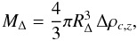 (A.1)where
 is the critical density of the Universe at
the cluster’s redshift z,
RΔ = cΔrs
is the radius within which the mean cluster overdensity is Δ times
ρc,z and the relation with the
concentration cΔ and the scale radius
rs holds by definition of the NFW mass profile. We assume
Δ = 200. Hereafter, we refer to Δ as any other assumed overdensity. In case it is referred
to the background density of the Universe,
ρb = Ωm,zρc,z,
it is straightforward to correct Δ by
is the critical density of the Universe at
the cluster’s redshift z,
RΔ = cΔrs
is the radius within which the mean cluster overdensity is Δ times
ρc,z and the relation with the
concentration cΔ and the scale radius
rs holds by definition of the NFW mass profile. We assume
Δ = 200. Hereafter, we refer to Δ as any other assumed overdensity. In case it is referred
to the background density of the Universe,
ρb = Ωm,zρc,z,
it is straightforward to correct Δ by 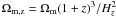 to
recover the definition in Eq. (A.1).
to
recover the definition in Eq. (A.1).
To convert the tabulated values to our definition of the
c − M relation,
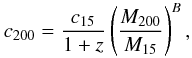 (A.2)where
 , we proceed as follows:
-
1.
by definition,
 is constant and
RΔ/cΔ
is fixed from the measurement of the scale radius. Therefore, we can write
is constant and
RΔ/cΔ
is fixed from the measurement of the scale radius. Therefore, we can write
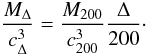 (A.3)
(A.3) -
2.
cΔ and c200 are related through the assumed NFW mass density profile
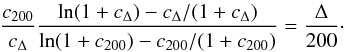 (A.4)This
function is monotonic and easily to resolve numerically to estimate
C = cΔ/c200,
that is a quantity that depends mostly on Δ and only marginally on the guessed
c200, as shown in Fig. A.1. For instance, for
(A.4)This
function is monotonic and easily to resolve numerically to estimate
C = cΔ/c200,
that is a quantity that depends mostly on Δ and only marginally on the guessed
c200, as shown in Fig. A.1. For instance, for  , which estimate the
virial overdensity predicted from the spherical collapse model in a flat Universe
with a contribution from dark energy (Eke et al. 2001), C = 1.34 and 1.22 at z = 0 and
z = 0.3, respectively, for Ωm = 0.3, with deviations
within 2% in the range c200 = 3 − 6.
, which estimate the
virial overdensity predicted from the spherical collapse model in a flat Universe
with a contribution from dark energy (Eke et al. 2001), C = 1.34 and 1.22 at z = 0 and
z = 0.3, respectively, for Ωm = 0.3, with deviations
within 2% in the range c200 = 3 − 6. -
3.
for a given relation
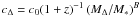 , we substitute the above
relations to obtain after simple algebrical operations:
, we substitute the above
relations to obtain after simple algebrical operations:
 (A.5)or
 (A.6)
(A.6)
Appendix B: Monte-Carlo realizations of the c200 − M200 relation
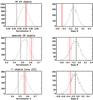 |
Fig. B.1 Distribution of the best-fit values of the normalization A and slope B after 10 000 MC realizations. The input values (in these plots from M08 / WMAP-5) are indicated with vertical solid (for all the simulated objects) and dashed (for the relaxed ones) lines. The red solid line represents the central value for the corresponding sample as quoted in Table 5. The red dotted lines show the 1σ uncertainties. |
We have run Monte-Carlo (MC) simulations to test the robustness of the observed
deviations in the c200 − M200
relation described in Sect. 5. We have used as input values the best-fit results (defined
in the following analysis as  and
and
 )
obtained in the numerical simulations from Neto et al. (2007; see their Eqs. (4) and (5)) and Macciò et al. (2008; see Table A1 and A2) and listed in Table 5. We have considered the results for both the complete sample and the
relaxed objects only. To each cluster in our sample with measured mass
M200,i and redshift
zi, we assign the concentration
c200,i defined as
)
obtained in the numerical simulations from Neto et al. (2007; see their Eqs. (4) and (5)) and Macciò et al. (2008; see Table A1 and A2) and listed in Table 5. We have considered the results for both the complete sample and the
relaxed objects only. To each cluster in our sample with measured mass
M200,i and redshift
zi, we assign the concentration
c200,i defined as ![Mathematical equation: \appendix \setcounter{section}{2} \begin{eqnarray} c_{200, i} & = & 10^{l_i} \\ l_i & = & \log_{10} \left[ \bar{c}_{15} \times \left(M_{200, i}/10^{15}\right)^{\bar{B}} / (1+z_i) \right] +R \times \epsilon_{\log c} \nonumber, \label{eq:mc} \end{eqnarray}](/articles/aa/full_html/2010/16/aa15271-10/aa15271-10-eq1271.png) (B.1)where
R is a random value extracted from a Gaussian distribution and
ϵlog c is the scatter in the log-Normal
distribution measured in the numerical simulations (~0.13 for samples including all the
simulated objects and ~0.1 for the sample of the relaxed ones; the actual values are
quoted in N07 and in Table A1 and A2 of M08). We assume that (1) our LEC objects follow
the distribution obtained for relaxed simulated clusters; (2) all the remaining clusters
follow the distribution estimated for the complete simulated halo sample; (3) the
3 samples considered in our analysis with 44, 26 and 11 clusters, respectively, are built
considering whether each object is a LEC and/or has an upper limit at 1σ
on the scale radius lower than Rsp, as discussed in Sect. 5.
To be conservative in our approach, we fit Eq. (5) to the distribution in the
c200 − M200 with the
fitexy technique that is the one that provides the most significant
deviations from the results obtained in numerical simulations. We repeat this process
10 000 times and obtain the plots shown in Fig. B.1
for each of the case investigated. In Table B.1, we
summarize our finding from which we conclude that, while the best-fit values estimated for
the samples of 26 and 11 clusters are within the overall distribution expected in
numerical simulations, the sample of 44 clusters provides results on the slope
B that lie on the lower end of the distribution, as probable
consequence of the uncertainties present both on the estimates of
c200 and M200 for the
18 clusters that are indeed not selected for the further analysis and on the residual bias
affecting the measurements of c200 under the hypothesis of the
hydrostatic equilibrium (see Sect. 5.1 and, e.g., Lau et al. 2009).
(B.1)where
R is a random value extracted from a Gaussian distribution and
ϵlog c is the scatter in the log-Normal
distribution measured in the numerical simulations (~0.13 for samples including all the
simulated objects and ~0.1 for the sample of the relaxed ones; the actual values are
quoted in N07 and in Table A1 and A2 of M08). We assume that (1) our LEC objects follow
the distribution obtained for relaxed simulated clusters; (2) all the remaining clusters
follow the distribution estimated for the complete simulated halo sample; (3) the
3 samples considered in our analysis with 44, 26 and 11 clusters, respectively, are built
considering whether each object is a LEC and/or has an upper limit at 1σ
on the scale radius lower than Rsp, as discussed in Sect. 5.
To be conservative in our approach, we fit Eq. (5) to the distribution in the
c200 − M200 with the
fitexy technique that is the one that provides the most significant
deviations from the results obtained in numerical simulations. We repeat this process
10 000 times and obtain the plots shown in Fig. B.1
for each of the case investigated. In Table B.1, we
summarize our finding from which we conclude that, while the best-fit values estimated for
the samples of 26 and 11 clusters are within the overall distribution expected in
numerical simulations, the sample of 44 clusters provides results on the slope
B that lie on the lower end of the distribution, as probable
consequence of the uncertainties present both on the estimates of
c200 and M200 for the
18 clusters that are indeed not selected for the further analysis and on the residual bias
affecting the measurements of c200 under the hypothesis of the
hydrostatic equilibrium (see Sect. 5.1 and, e.g., Lau et al. 2009).
All Tables
All Figures
|
Fig. 1 (Left) Surface brightness profile in the 0.7−1.2 keV band (black filled circles) of Abell1835 compared with the profiles of the background components. The open diamonds show the count rate predicted from the background spectral model in the annulus 10–12 arcmin and rescaled for the mean vignetting correction of 0.472 at those radii: the instrumental component (NXB; green), the photon component (CXB + galactic foregrounds; blue) and the total background (sky + instrumental; red). The dashed lines show the background profiles that we have used in our analysis: the “photon” background (blue), which is constant and corresponds to the value in the outer annulus rescaled to the center, and the instrumental background profile (green), increasing with radius in order to consider the over-correction of this component. The red dashed line shows the total background that we have subtracted from our source plus background profile, with its associated one σ statistical error (red dotted lines) obtained with a Monte Carlo simulation. Note that the intensity of the background components and their relative contribution vary significantly from cluster to cluster. (Right) Example of the PSF-corrected background-subtracted surface brightness profile as obtained after the analysis outlined in Sect. 2.2. This example refers to Abell1835, one of the objects with the largest smearing effect due to the combination of the telescope’s PSF and the centrally peaked intrinsic profile. |
| In the text | |
|
Fig. 2 Example of the results of the two analyses adopted for the mass reconstruction.
(Top and middle panels, left) Gas density profile as obtained
from the deprojection of the surface brightness profile compared to the one
recovered from the deprojection of the normalizations of the thermal model in the
spectral analysis; observed temperature profile with overplotted the best-fit model
(from Method 1). (Top and middle panels, right)
Data (diamonds) and models (dashed lines) of the projected gas density
squared and temperature (from Method 2). (Bottom, left)
Constraints in the rs − c
plane with the prediction (in green) obtained by imposing the relation
|
| In the text | |
|
Fig. 3 (First 2 panels on the left) Relative errors on M200 (black) and c200 (red) estimated by the two methods. The median values are indicated by a dashed line. (3rd and 4th panel from left) Ratios between the best-fit result on the scale radius rs (3rd panel) and on R500 (4th panel) and outermost radius reached with the spatial analysis. |
| In the text | |
|
Fig. 4 Best-fit values of rs, c, gas mass fraction fgas at R500 and dark mass MDM within R200 as obtained from Method 1 (diamonds; the ones including red points indicate the objects where the condition (rs + ϵrs) < Rsp is satisfied by both methods. Rsp here plotted as horizontal line in the upper panel). |
| In the text | |
|
Fig. 5 Estimates of M200 (left), c200 (center) and fgas(<R500) (right) with the two methods. (Upper panels) The color code indicates the objects at z < 0.15 (blue), in the range 0.15 < z < 0.25 (green) and at z > 0.25 (red). (Lower panels) Distribution of Low (LEC), Medium (MEC), High (HEC) Entropy Core systems. |
| In the text | |
|
Fig. 6 Data in the plane (c200,M200) used to constrain the cosmological parameters (Ωm,σ8). The dotted lines show the predicted relations from Eke et al. (2001) for a given ΛCDM cosmological model at z = 0 (from top to bottom: σ8 = 0.9 and σ8 = 0.7). The shaded regions show the predictions in the redshift range 0.1 − 0.3 for an assumed cosmological model in agreement with WMAP-1, 5 and 3 years (from the top to the bottom, respectively) from Bullock et al. (2001; after Macciò et al. 2008). The dashed lines indicate the best-fit range at 1σ obtained for relaxed halos in a WMAP-5 years cosmology from Duffy et al. (2008; thin lines: z = 0.1, thick lines: z = 0.3). Color codes and symbols as in Fig. 5. |
| In the text | |
|
Fig. 7 Cosmological constraints in the
(Ωm,σ8) plane obtained from
Eqs. (6) and (7) by using predictions from the model by
Eke et al. (2001). The confidence contours at
1,2,3σ on 2 parameters (solid
contours) are displayed. The combined likelihood with the probability distribution
provided from the cluster gas mass fraction method is shown in red. The dashed green
line indicates the power-law fit |
| In the text | |
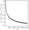 |
Fig. A.1 Numerical solution to Eq. (A.4) for an assumed c200 in the range 3–8 (from the thinnest to the thickest line). |
| In the text | |
|
Fig. B.1 Distribution of the best-fit values of the normalization A and slope B after 10 000 MC realizations. The input values (in these plots from M08 / WMAP-5) are indicated with vertical solid (for all the simulated objects) and dashed (for the relaxed ones) lines. The red solid line represents the central value for the corresponding sample as quoted in Table 5. The red dotted lines show the 1σ uncertainties. |
| In the text | |
Current usage metrics show cumulative count of Article Views (full-text article views including HTML views, PDF and ePub downloads, according to the available data) and Abstracts Views on Vision4Press platform.
Data correspond to usage on the plateform after 2015. The current usage metrics is available 48-96 hours after online publication and is updated daily on week days.
Initial download of the metrics may take a while.