| Issue |
A&A
Volume 674, June 2023
|
|
|---|---|---|
| Article Number | A48 | |
| Number of page(s) | 19 | |
| Section | Cosmology (including clusters of galaxies) | |
| DOI | https://doi.org/10.1051/0004-6361/202243922 | |
| Published online | 29 May 2023 | |
Constraining the mass and redshift evolution of the hydrostatic mass bias using the gas mass fraction in galaxy clusters⋆
Université Paris-Saclay, CNRS, Institut d’Astrophysique Spatiale, 91405 Orsay, France
e-mail: This email address is being protected from spambots. You need JavaScript enabled to view it.
Received:
2
May
2022
Accepted:
12
March
2023
Abstract
The gas mass fraction in galaxy clusters is a convenient probe to use in cosmological studies, as it can help derive constraints on a range of cosmological parameters. This quantity is, however, subject to various effects from the baryonic physics inside galaxy clusters, which may bias the obtained cosmological constraints. Among different aspects of the baryonic physics at work, in this paper we focus on the impact of the hydrostatic equilibrium assumption. We analyzed the hydrostatic mass bias B, constraining a possible mass and redshift evolution for this quantity and its impact on the cosmological constraints. To that end, we considered cluster observations of the Planck-ESZ sample and evaluated the gas mass fraction using X-ray counterpart observations. We show a degeneracy between the redshift dependence of the bias and cosmological parameters. In particular we find evidence at 3.8σ for a redshift dependence of the bias when assuming a Planck prior on Ωm. On the other hand, assuming a constant mass bias would lead to the extremely large value of Ωm > 0.860. We show, however, that our results are entirely dependent on the cluster sample under consideration. In particular, the mass and redshift trends that we find for the lowest mass-redshift and highest mass-redshift clusters of our sample are not compatible. In addition, we show that assuming self-similarity in our study can impact the results on the evolution of the bias, especially with regard to the mass evolution. Nevertheless, in all the analyses, we find a value for the amplitude of the bias that is consistent with B ∼ 0.8, as expected from hydrodynamical simulations and local measurements. However, this result is still in tension with the low value of B ∼ 0.6 derived from the combination of cosmic microwave background primary anisotropies with cluster number counts.
Key words: large-scale structure of Universe / cosmological parameters / galaxies: clusters: general / methods: data analysis / galaxies: clusters: intracluster medium / X-rays: galaxies: clusters
Full Table A.1 is only available at the CDS via anonymous ftp to https://cdsarc.cds.unistra.fr (130.79.128.5) or via https://cdsarc.cds.unistra.fr/viz-bin/cat/J/A+A/674/A48
© The Authors 2023
 Open Access article, published by EDP Sciences, under the terms of the Creative Commons Attribution License (https://creativecommons.org/licenses/by/4.0), which permits unrestricted use, distribution, and reproduction in any medium, provided the original work is properly cited.
This article is published in open access under the Subscribe to Open model. This email address is being protected from spambots. You need JavaScript enabled to view it. to support open access publication.
1. Introduction
Galaxy clusters are the most massive gravitationally bound systems of our Universe. As such they contain a wealth of cosmological and astrophysical information. They can be used either as powerful cosmological probes (White et al. 1993; Allen et al. 2011) or as astrophysical objects of study to better characterise the physics of the intra-cluster medium (ICM; Sarazin 1988) and how these structures are connected to the rest of the cosmic web. Constraints on the matter density, Ωm, or the amplitude of the matter power spectrum, σ8, can be inferred from several galaxy cluster observables. We could, for instance, use cluster number counts, their clustering, or the properties of their gas content to constrain cosmological parameters (see e.g., Allen et al. 2011 or Kravtsov & Borgani 2012 for reviews). Among the more recent probes, we can also cite the cluster sparsity (Balmés et al. 2013).
The baryon budget of these objects is also interesting in terms of the aspect of galaxy clusters as cosmological probes and especially the hot gas of the ICM that composes the major part of the baryonic matter inside clusters (Gouin et al. 2022). Indeed the gas mass fraction of galaxy clusters, fgas, is considered to be a good proxy for the universal baryon fraction (Borgani & Kravtsov 2011) and can be used to constrain cosmological parameters including the matter density, Ωm, the Hubble parameter, h, the dark energy density, ΩDE, or the equation of state of dark energy w (see e.g., Allen et al. 2008; Holanda et al. 2020; Mantz et al. 2022 and references therein).
The gas content inside galaxy clusters is, however, also affected by baryonic physics. Such baryonic effects need to be taken into account while performing the cosmological analysis, as they introduce systematic uncertainties in the final constraints (see e.g., the discussions from McCarthy et al. 2003a,b; Poole et al. 2007; Hoekstra et al. 2012; Mahdavi et al. 2013; Ruan et al. 2013; Sakr et al. 2018).
For instance, feedback mechanisms inside clusters, such as active galactic nuclei (AGN) heating, can drive gas out of the potential wells, resulting in slightly gas-depleted clusters. This depletion of galaxy clusters’ gas with respect to the universal baryon fraction is accounted for by the depletion factor Υ (Eke et al. 1998; Crain et al. 2007). This depletion factor has been thoroughly studied in hydrodynamical simulations throughout the years, in clusters (Kravtsov et al. 2005; Planelles et al. 2013; Sembolini et al. 2016; Henden et al. 2020, and references therein) as well as in filaments (Galárraga-Espinosa et al. 2022). As a result, this parameter can be very well constrained and robustly predicted in numerical simulations. Secondly, galaxy clusters are often assumed to be in hydrostatic equilibrium (HE hereafter). Nevertheless, non-thermal processes such as turbulence, bulk motions, magnetic fields or cosmic rays (Lau et al. 2009; Vazza et al. 2009; Battaglia et al. 2012; Nelson et al. 2014; Shi et al. 2015; Biffi et al. 2016), might cause a departure from the equilibrium condition in the ICM. Therefore, the HE assumption leads to cluster mass estimations biased toward lower values with respect to the total cluster mass. The impact of non-thermal processes, and therefore an evaluation for the bias in the cluster mass estimation, was first considered in hydrodynamical simulations (Rasia et al. 2006). Since then, a parametrization for this mass bias has been introduced also in observations, for instance when detecting clusters in X-ray or millimeter wavelengths, the latter exploiting the thermal Sunyaev-Zeldovich effect (Sunyaev & Zeldovich 1972, tSZ hereafter; see Pratt et al. 2019 for a review). We stress that this bias affects all the observables which might assume hydrostatic equilibrium when evaluating cluster masses and, thus, the gas mass fraction. Throughout the paper we define this mass bias as B = MHE/Mtot.
If the depletion factor is well constrained and understood, this is not the case for the hydrostatic mass bias as its value is still under debate. In a number of analyses including weak lensing works (Weighing the Giants (WtG), von der Linden et al. 2014; the Canadian Cluster Comparison Project (CCCP), Hoekstra et al. 2015; Okabe & Smith 2016; Sereno et al. 2017), tSZ number counts (Salvati et al. 2019), X-ray observations (Eckert et al. 2019), or hydrodynamical simulations (McCarthy et al. 2017; Bennett & Sijacki 2022), this mass bias is estimated to be around B ∼ 0.8 − 0.85. The works from Planck Collaboration XX (2014), Planck Collaboration XXIV (2016) however show that to alleviate the tension on the amplitude of the matter power spectrum, σ8, between local and cosmic microwave background (CMB hereafter) measurements, a much lower B is needed. Indeed, when combining CMB primary anisotropies and tSZ cluster counts, CMB measurements drive the constraining power on the cosmological parameters and, thus, on the bias, favoring a bias B ∼ 0.6 − 0.65. This result was confirmed later on by Salvati et al. (2018) and Planck Collaboration VI (2020). In addition, the study from Salvati et al. (2018) shows that when forcing B = 0.8 while assuming a Planck cosmology, the observed cluster number counts are way below the number counts predicted using the CMB best-fit cosmological parameters. In other words, when assuming B = 0.8 with a CMB cosmology, one predicts approximately thrice as many clusters as what is actually observed.
As the precise value of the mass bias is still an open matter and has a direct impact on the accuracy and precision of the cosmological constraints deduced from galaxy clusters, we propose a new and independent measurement of this quantity. In this paper we use the gas mass fractions of 120 galaxy clusters from the Planck-ESZ sample Planck Collaboration VIII (2011) to bring robust constraints on the value of the hydrostatic bias. More importantly, we aim at studying the potentiality of variations of the bias with mass and redshift. Such studies on mass and redshift trends of B have already been carried out in works using weak lensing (von der Linden et al. 2014; Hoekstra et al. 2015; Smith et al. 2016; Sereno & Ettori 2017) or tSZ number counts (Salvati et al. 2019), sometimes giving contradictory results. In this work we measure and use gas mass fractions from a sample to get new independent constraints on B as well as on its mass and redshift evolution. This study is also aimed at investigating the role that an evolution of the bias would have on the cosmological constraints we obtain from fgas data.
After describing the theoretical modelling and our cluster sample in Sect. 2, we detail our methods for the data analysis in Sect. 3. We show our results in Sect. 4, first focussing on the effect of assuming a varying bias on our derived cosmological constraints, then looking at the sample dependence of our results. Finally, we discuss our results in Sect. 5 and draw our conclusions in Sect. 6. Throughout the paper, we assume a reference cosmology with H0 = 70 km s−1 Mpc−1, Ωm = 0.3 and ΩΛ = 0.7.
2. Theoretical modelling and data
2.1. Gas fraction sample
The gas mass fraction is defined as the ratio of the gas mass over the total mass of the cluster:
 (1)
(1)
Using X-ray observations, the gas mass is obtained by integrating the density profile ρ(r) inside a certain radius, r, as shown in Eq. (2) below
 (2)
(2)
Here, the density profile ρ(r) is obtained from the electron density profile ne(r), measured from X-ray observations. We have:
 (3)
(3)
where μ is the mean molecular weight, mp the proton mass, ne the electron number density, and np the proton number density with ne = 1.17np in a fully ionised gas. Using the density profile and a temperature profile, T(r), the total hydrostatic mass, MHE, can be computed by solving the hydrostatic equilibrium equation shown below:
 (4)
(4)
where kB is the Boltzmann constant and G is the gravitational constant.
Similarly to the gas mass and the hydrostatic mass, the cluster gas mass fraction is evaluated within a characteristic radius, determined by the radius of the mass measurements. We define this radius, RΔ, as the radius that encloses Δ times the critical density of the Universe, ρc = 3H2/8πG. The gas content inside galaxy clusters is affected by baryonic physics and the impact of the different astrophysical processes might depend on the considered cluster radius, RΔ. In this work, we focus on gas fractions taken at R500, and from now on all the quantities we consider are taken at R500. We note that this radius is larger than most studies using the gas fraction of galaxy clusters as a cosmological probe, which are generally carried out at R2500 (Allen et al. 2002, 2008, 2011; Mantz et al. 2014; Holanda et al. 2020; Mantz et al. 2022). We briefly discuss this choice of radius in Sect. 5.2.2.
We computed the gas fraction for the clusters in the Planck-ESZ survey (Planck Collaboration VIII 2011). In particular, we considered 120 out of 189 clusters of the Planck-ESZ sample, for which we have follow-up X-ray observations by XMM-Newton up to R500 (here called the ESZ sample for simplicity). Our sample therefore spans a total mass range from 2.22 × 10¹⁴ M⊙ to 1.75 × 10¹⁵ M⊙ and redshift range from 0.059 to 0.546. We started from the gas and total masses of the clusters derived in Lovisari et al. (2020a). We refer to their work for the detailed analysis of the mass evaluation. We just stress here that the total cluster masses were obtained assuming hydrostatic equilibrium, as shown in Eq. (4), thus inducing the presence of the hydrostatic mass bias. From these gas masses and hydrostatic masses, we computed the gas fraction following Eq. (1) to find that they are within the range [0.06, 0.20]. We note that there are correlations between the gas mass and hydrostatic mass measurements. These correlations induce a corrective term when computing the error bars of fgas. We check that this correlation term (provided by Lorenzo Lovisari, priv. comm.) introduces a negligible contribution to the total error budget. We propagate the asymmetric errors from the mass measurements to obtain the uncertainty on fgas. We also note that the Malmquist bias may affect our final results; however, the discussions in Lovisari et al. (2020a) and Andrade-Santos et al. (2021) show that this effect is negligible in the case of this sample.
We give the redshifts, gas masses, hydrostatic masses and gas fractions of the clusters from our sample in Table A.1 in the appendix. We show in Fig. 1 the observed gas fraction in this sample, with respect to redshift and mass. We also compare these fgas values to the universal baryon fraction Ωb/Ωm = 0.156 ± 0.03 from Planck 2018 results (Planck Collaboration VI 2020).
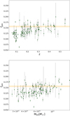 |
Fig. 1. Gas mass fraction of Planck-ESZ clusters with respect to redshift (top) and with respect to cluster mass (bottom). The yellow bands in both plots mark the Planck Collaboration VI (2020) value of Ωb/Ωm = 0.156 ± 0.003. |
2.2. Modelling of the observed gas fraction
The hydrostatic mass is used to evaluate the total cluster mass, yet it is biased low with respect to the true total mass by a factor B = MHE/Mtrue. The measured gas mass fraction is thus:
 (5)
(5)
Besides the hydrostatic mass bias, the measured gas fraction depends on a variety of instrumental, astrophysical, and cosmological effects. One way of quantifying these effects is to compare the gas fraction we obtain from gas mass and hydrostatic mass measurements to the theoretical (hydrostatic) gas fraction we expect from Eq. (6) below, from Allen et al. (2008). In this equation (and in the rest of the paper), the quantity noted as Xref is the quantity X in our reference cosmology:
 (6)
(6)
Here, K is an instrumental calibration correction. We take K = 1 ± 0.1 from Allen et al. (2008) and discuss the soundness of this assumption in Sect. 5.1.1. Regarding the astrophysical contributions, Υ(M, z) is the baryon depletion factor, describing how baryons in clusters are depleted with respect to the universal baryon fraction and B(M, z) is the hydrostatic mass bias we discuss above. Finally Ωb/Ωm is the universal baryon fraction, DA is the angular diameter distance, f* is the stellar fraction, and A(z) is an angular correction which we show in Eq. (7):
![Mathematical equation: $$ \begin{aligned} A(z) = \left(\frac{\theta _{500}^\mathrm{ref}}{\theta _{500}} \right)^\eta \simeq \left( \frac{H(z)D_A(z)}{\left[H(z)D_A(z) \right]^\mathrm{ref}} \right)^\eta . \end{aligned} $$](/articles/aa/full_html/2023/06/aa43922-22/aa43922-22-eq7.gif) (7)
(7)
The parameter η accounts for the slope of the fgas profiles enclosed in a spherical shell. Here we take η = 0.442 from Mantz et al. (2014). With A(z) being, however, very close to one for realistic models and within our range of parameters, the value of this parameter has a negligible impact on our results.
We note that this model is valid as long we are assuming self-similarity, which we do here. Deviations from self-similarity may induce supplementary dependencies. We thus discuss our hypothesis in Sect. 5.1.2 and Appendix B.
3. Methods
Our purpose in this work is to use the gas mass fraction of galaxy clusters to constrain the value of the hydrostatic mass bias and, in particular, its evolution with mass and redshift. We also want to study the role of such an evolution of the bias on the subsequent cosmological constraints derived from fgas data. We recall here that all constraints derived from gas mass fraction data are obtained by comparing the measured gas fraction to the theoretical gas fraction expected from Eq. (6), which is proportional to the universal baryon fraction. Besides this proportionality, all the other constraints are deduced as corrections needed to match the observed fgas in clusters to the constant Ωb/Ωm. As discussed in Sect. 2, one of these correction terms accounts for the baryonic effects taking place in the ICM. These baryonic effects are accounted for by the depletion factor Υ(M, z) and the hydrostatic bias B(M, z), which we are interested in. As shown in Eq. (6), we cannot constrain independently B(M, z) and Υ(M, z), as the two parameters are strongly degenerated. What we have access to instead is the ratio of the two quantities, Υ(M, z)/B(M, z). In order to break this degeneracy and properly constrain the bias, strong constraints on the depletion factor and its evolution with mass and redshift are required. Obtaining such results is however out of the scope of this paper, and we retrieve these constraints from hydrodynamical simulations works.
The depletion factor is known to vary with mass, however this evolution is particularly strong for groups and low mass clusters (< 2.1014 M⊙) while it becomes negligible at the high masses we consider (see the discussion in Sect. 3.1.1 of Eckert et al. 2019 based on results from The Three Hundred Project simulations; Cui et al. 2018). Works from Planelles et al. (2013) and Battaglia et al. (2013) also show that the depletion factor is constant with redshift when working at R500. Throughout the paper, we thus assume a constant depletion factor with mass and redshift Υ0 = 0.85 ± 0.03, based on hydrodynamical simulations from Planelles et al. (2013).
3.1. Bias evolution modelling
In order to analyze a possible mass and redshift evolution of the mass bias, we consider a power law evolution for the hydrostatic bias, with pivot masses and redshifts set at the mean values of the considered cluster sample:
 (8)
(8)
with B0 as the amplitude.
We chose this model for the sake of simplicity following what is done in Salvati et al. (2019), as the exact dependence of B on mass and redshift is not known. In Sect. 5.1.3 we discuss the role of this parametrization by comparing our results with a linear evolution of B, and find results similar to those of the power law description. The complete likelihood function thus writes, assuming no deviation from self-similarity:
 (9)
(9)
where
 (10)
(10)
with σi as the uncertainties on the gas fraction data and fgas, Th as the gas fraction expected from Eq. (6). The parameter σf is the intrinsic scatter of the data, which we treat as a free parameter.
3.2. Free cosmology study
In the first part of our analysis we simply assess the necessity to consider an evolving bias, by looking at the impact of assuming such a variation on the subsequent cosmological constraints. To do so, we compare the posterior distributions in three different cases: In the first case we let free the baryon fraction, Ωb/Ωm, the matter density, Ωm, and the parameters accounting for the variation of the bias α, β, and B0. We refer to this scenario as ‘VB’. In the second case we let free only the cosmological parameters and fix the bias parameters to α = 0 and β = 0, resulting in a constant bias at the value B0. This scenario will be noted in the rest of the paper as ‘CB’. Due to a degeneracy between β and Ωm which we discuss later on, we also look at our results when leaving the set of parameters (B0, α, β, Ωb/Ωm) free but assuming a prior on Ωm, in order to break this degeneracy and constrain β more accurately. We call this scenario ‘VB + Ωm’.
The set of parameters for which we assume flat priors in this part of the study is thus (B0, α, β, Ωb/Ωm, Ωm, σf), as we show in the first column of Table 1. This work is performed on the entirety of our cluster sample, for which our mean mass and redshift are:
 (11)
(11)
Set of priors used in our analysis.
Throughout this whole part of the analysis, we consider a prior on the total value of the bias for a certain cluster mass and redshift, taken from the Canadian Cluster Comparison Project – Multi Epoch Nearby Cluster Survey (CCCP-MENeaCS) analysis (Herbonnet et al. 2020):

where zCCCP = 0.189 and MCCCP = 6.24 × 10¹⁴ M⊙ are the mean mass and redshift for the CCCP-MENeaCS sample.
3.3. Sample dependence tests
In the second part, we looked into possible sample dependencies of our results regarding the value of the bias parameters B0, α, and β. To that end, we focus on different subsamples within the main sample, based on mass and redshift selections. Matching the selection from weak lensing studies such as the Comparing Masses in Literature (COMALIT; Sereno & Ettori 2017) or Local Cluster Substructure Survey (LOCUSS; Smith et al. 2016) studies, we operate a redshift cut at z = 0.2, differentiating clusters that are above or below this threshold value. This choice was also motivated by the results from Salvati et al. (2019), investigating the hydrostatic mass bias from the perspective of tSZ number counts. Their study showed that the trends in the mass bias depended on the considered redshift range, with results changing when considering only clusters with z > 0.2. We also performed a mass selection, differentiating between the clusters that are above or below the median mass of the sample Mmed = 5.89 × 10¹⁴ M⊙.
In summary, the samples we consider in this study are the following:
The full sample of 120 clusters, with the mean mass and redshift given previously in Eq. (11). The second subsample is composed of clusters with z < 0.2 and M < 5.89 × 10¹⁴ M⊙. We consider them in the ‘low Mz’ subsample, which contains 47 clusters. The mean mass and redshift are
 (12)
(12)
Finally our third subsample is constituted of clusters with z > 0.2 and M > 5.89 × 10¹⁴ M⊙. We consider them in the ‘high Mz’ subsample, which contains 45 clusters. The mean mass and redshift are
 (13)
(13)
We did not consider the ‘low z–high M’ and ‘high z–low M’ subsamples as by construction they do not contain enough clusters (15 and 13, respectively) to obtain meaningful results. For illustration purposes, we show in Fig. 2 the binned mass-redshift plane of our sample, with the delimitation of the different subsamples. Inside each bin, we computed the mean value of fgas if at least one cluster is inside the bin.
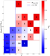 |
Fig. 2. Binned mass-redshift plane of the Planck-ESZ sample. Inside each bin we compute the mean value of fgas. We show the number of clusters included in each bin and mark the delimitation of each subsample. |
To carry out this study of the sample dependence, we compared the posterior distributions obtained when running our MCMC on the three aforementioned samples independently. We note that we kept the prior on Ωm for this part of the study, and that we add a prior on Ωb/Ωm. This choice is motivated by the presence of a degeneracy between the baryon fraction and the amplitude of the bias B0. This degeneracy is broken in the first part of the analysis by assuming a prior on the total value of the bias. However, when trying to compare all the bias parameters between samples (including the amplitude), we do not wish to be dependent on such a prior. The universal baryon fraction being well known and constrained, such a prior is a convenient way to break the degeneracy between Ωb/Ωm and B0 and still obtain meaningful results on the value of all the bias parameters. The set of parameters following flat priors in this part of the study is thus (B0, α, β, σf), as we show in the second column of Table 1.
In brief, we adopted the list of priors given in Table 1 to constrain the parameters used to describe our fgas data. We fit our model in Eq. (6) to the fgas data with an MCMC approach using the sampler emcee (Foreman-Mackey et al. 2013). We note that the prior we consider on f* = 0.015 ± 0.005 coming from Eckert et al. (2019) has close to no effect on our final results, as this term in Eq. (6) is almost negligible.
4. Results
4.1. Bias evolution study
In the first part of this analysis, we intend on studying the possibility of an evolution of the hydrostatic mass bias with cluster mass and redshift. To that end, we compare the cosmological constraints obtained on the full sample when considering a constant bias to those obtained when leaving the bias free to vary. Our results are summed up in Fig. 3 and in Table 2.
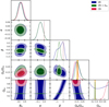 |
Fig. 3. 1D and 2D posterior distributions for the CB, VB, and VB + Ωm scenarios. The contours mark the 68% and 95% confidence level (c.l.). The gray dashed lines highlight reference values for (α, β, Ωb/Ωm, Ωm)=(0, 0, 0.156, 0.315). The orange bands mark the Planck Collaboration VI (2020) values for Ωb/Ωm and Ωm at 2σ c.l. |
Constraints obtained on bias and cosmological parameters in the CB, VB and VB + Ωm scenarios.
In the VB case, namely when leaving the set of parameters (B0, α, β, Ωb/Ωm, Ωm, σf) free with a prior on the total value of B, we show that a mass-independent bias seems to be favored. Indeed, with α = −0.056 ± 0.037 we remain compatible with 0 within 2σ, even though the peak is slightly lower. We also show that our derived Ωb/Ωm is fully compatible with the Planck Collaboration VI (2020) value, since we obtained  . We cannot, however, bring such constraints on β and Ωm, as these two parameters are heavily degenerated. We zoom in on this degeneracy in Fig. 4 and show that higher values of β call for higher values of Ωm. This degeneracy can be explained by the fact that both parameters entail a redshift dependence on the part of the gas fraction. Indeed, Ωm intervenes in the computation of DA(z) and H(z), which entirely drive the sensitivity of fgas to cosmology. We thus argue that this degeneracy between β and Ωm (which we show here in a simple Flat-ΛCDM model) could also be observed between β and any other cosmological parameter, as long as they appear in the computation of DA(z) or H(z). As a side note, we show a slight degeneracy between the baryon fraction Ωb/Ωm and β, with a lower Ωb/Ωm implying a higher, closer to 0 β. This degeneracy is caused by the combined effect of the degeneracy between β and Ωm, and the degeneracy between Ωb/Ωm and Ωm, which is expected (shown in Fig. 3).
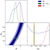 |
Fig. 4. Posterior distributions showing the degeneracy between β and Ωm. The contours mark the 68% and 95% c.l. The gray dashed lines highlight reference values for (β, Ωm)=(0, 0.315). The orange band marks the Planck Collaboration VI (2020) value for Ωm at 2σ c.l. |
As the matter density, Ωm, has been strongly constrained in a number of works, we chose to assume the Planck Collaboration VI (2020) prior shown in Table 1 on this parameter to break its degeneracy with β, in the VB + Ωm scenario. The effect of this prior is negligible on the constraints on α and Ωb/Ωm, as we obtain α = −0.057 ± 0.038 and  , fully compatible with the results obtained without this prior. On the other hand, the use of this prior allows us to constrain β. We show that the hydrostatic bias seems to show a strong redshift dependence, with β = −0.64 ± 0.18. This value of β < 0 would mean a value of B decreasing with redshift, that is to say, more and more biased masses toward higher redshifts. We also note a slight degeneracy between α and β, but this is most probably due to selection effects of the sample. As the higher redshift clusters tend to mostly have higher masses (see Fig. 2), a redshift trend of the bias could then be interpreted as a slight mass trend, explaining this degeneracy. These selection effects causing the degeneracy are those we explore in the second part of the analysis when looking at the sample dependence of the results (see Sect 4.2).
The effect of assuming a constant bias (α = β = 0) in the CB case does not have a strong impact on our constraints on Ωb/Ωm, which peaks just slightly below the Planck value, but does remain compatible, with  . B0 is slightly above yet compatible with the value found in the varying bias case, with B0 = 0.842 ± 0.040. This is simply caused by the fact that for a constant bias the amplitude B0 is now completely determined by the total value of the bias B(zCCCP, MCCCP). On the other hand, due to the degeneracy between β and Ωm, imposing no redshift evolution of the bias requires a very high matter density, resulting in Ωm > 0.860, fully incompatible with the Planck value. Such a high matter density is not expected in current standard cosmology and is totally aberrant. We note that these results do not completely rely on our prior on the total value of the bias. Indeed, we also performed our analysis while assuming a prior from the first results of the CCCP analysis (Hoekstra et al. 2015):
 (14)
(14)
with (〈z〉,〈M〉) = (0.246,14.83 × 1014 h−1 M⊙). Our constraints when considering this prior do not change with respect to B(zCCCP, MCCCP)=0.84 ± 0.04, except a small shift on  in the CB case.
As such, we show that we need to assume an evolution of the hydrostatic mass bias, at least in redshift, to properly describe our fgas data. In the rest of our study we focus on exploring the bias evolution. We thus consider only the VB + Ωm scenario, to be able to constrain β despite its degeneracy with the matter density. We also assume a Planck Collaboration VI (2020) prior on Ωb/Ωm, as the universal baryon fraction is degenerated with the total value of the bias (see Eq. (6)). The bias parameters (B0, α, β) are thus left free and we chose not to use a prior on the total value of B going forward.
4.2. Sample dependence of the results
If an evolution of the bias seems necessary to properly constrain cosmological parameters using fgas data at R500, the strength of this evolution might differ depending on the masses and redshifts of the clusters we consider. We thus repeat the previous study, this time focusing only on the bias parameters, using the previously defined LowMz and HighMz subsamples in addition to the full sample. We recall that in this section, we are considering the VB + Ωm scenario, with an additional prior on Ωb/Ωm. The summary of our results is given in Table 3 and in Figs. 5 and 6.
Constraints obtained on the bias parameters depending on the considered sample.
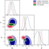 |
Fig. 5. 1D and 2D posterior distributions for the bias parameters in the three mass- and redshift-selected samples. The levels of the contours mark the 68% and 95% confidence levels. Gray dashed lines mark the reference values (α, β)=(0, 0). |
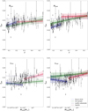 |
Fig. 6. Fits obtained from our analysis, for the different mass- and redshift-selected samples. The results in the top two panels are represented with respect to redshift at constant mass (respectively minimal and maximal masses of the full sample), while the bottom two panels are the results presented with respect to mass, at a fixed redshift (respectively minimal and maximal redshifts of the full sample). The shaded areas around the curves mark the 68% and 95% confidence levels. The blue dashed line marks the reference value Ωb/Ωm = 0.156. |
Our results when considering the full sample are (as expected) the same as when adopting flat priors on the cosmological parameters. The only slight exception is B0, peaking slightly higher due to the absence of a prior on the total bias. We find an amplitude of B0,full = 0.840 ± 0.095. The parameters accounting for the bias evolution remain unchanged, with αfull = −0.057 ± 0.038 and βfull = −0.64 ± 0.18. Thus, our results remain compatible with no mass evolution of the bias but still find a strong hint for a redshift dependence.
If all subsamples provide compatible values for the amplitude with  , B0, HighMz = 0.767 ± 0.086 and B0,full =〈0.840 ±〈0.095, this cannot be said regarding α and β. Indeed, if the study of the full sample seems to suggest no mass evolution and a mild redshift trend of the bias, we observe the reverse behavior in the HighMz subsample. With αhighMz = − 0.149 ± 0.058 and βHighMz = − 0.08 ± 0.23, the preferred scenario would be the one of B constant with redshift, yet decreasing with cluster mass. On the other end of the mass-redshift plane, the results show exactly the opposite evolution, in agreement with the constraints from the full sample but aggravating the trends. With αLowMz = 0.09 ± 0.11 and
  , we show we are fully compatible with no mass evolution of the bias, even with the posterior of α peaking slightly above 0 contrary to the other samples. More importantly, we show a strong decreasing trend of B with redshift, as we obtain β peaking close to −1. We note that the posterior distribution for this subsample is quite wider than it is for the full sample or the HighMz subsample. This is due to the smaller mass and redshift range of this sample (see Fig. 2), diminishing its constraining power with respect to the other two selections. This is, however, sufficient to highlight a redshift dependence of the bias when considering the least massive clusters of our sample at the lowest redshifts.
In Fig. 6, we show what these values of the bias parameters translate to in terms of the gas fraction with respect to redshift and mass. We show these fits computed at [Mmin, Mmax] with z free and at [zmin, zmax] with M free, taking into account the uncertainties at 68% and 95% c.l. We first notice what was highlighted in the contours of Fig. 5, which is that the results obtained for the full sample mainly fall in between the two extreme cases of the LowMz and HighMz subsamples. Secondly we show that the incompatibility between the two smaller subsamples is fully visible in the result of the fits. In the bottom two panels showing the fgas(M) relation, the LowMz and HighMz even seem to exhibit opposite trends, similarly to what is seen in Fig. 5. Finally, we note an offset in the relative positions of the curves for the two subsamples, depending on mass and redshift. This is simply due to the fact that our model describes a simultaneous evolution of the bias both with mass and redshift, which happens to be non-zero in our case.
In summary, we claim to have found strong evidence for the sample dependence of our results regarding the mass and redshift evolution of the hydrostatic mass bias. Such a sample dependence had already been noted in other works studying the evolution of the bias using tSZ cluster counts, but not when using fgas data.
5. Discussion
As we have shown in the previous section, considering an evolution of the bias seems to be necessary to infer sensible cosmological constraints. On the other hand, the variation of the bias that we measure is very dependent on the sample we consider, as we show different trends of the bias depending on mass and redshift selections inside our main sample. We discuss these results here, trying to take into account all the systematic effects that could appear and bias our results. We also compare our findings to previous studies focused on the bias and its evolution, from different probes.
5.1. Possible sources of systematic effects
5.1.1. Instrumental calibration effects
All of the masses used in this work were taken from Lovisari et al. (2020a), where the authors used XMM-Newton observations. Possible calibration effects may have impacted the mass measurements in their work and induced biases (see e.g., Mahdavi et al. 2013 or Schellenberger et al. 2015) This effect has been taken into account under the form of a K = 1.0 ± 0.1 parameter in our analysis, but we try here to check if this assumption is sound. The clusters of the Planck-ESZ sample have also been observed using Chandra, in Andrade-Santos et al. (2021). From their work, we retrieved their total masses and compare them to the XMM-Newton masses. The result of the comparison is shown in Fig. 7. We performed a fit of the point cloud in the log-log space, assuming a linear model of the form log(MXMM)=alog(MChandra)+b. Similarly to the model we defined in Eq. (8) when studying the evolution of the bias, we set a pivot to the mean value of the Chandra masses, 〈MChandra = 6.32 × 10¹⁴ M⊙. We note that the results we present below do not change when putting the pivot at the median mass instead of the mean. To perform the fit of the point cloud we resorted to an MCMC, in order to be able to account for the asymmetric measurement errors both in X and Y axis and the intrisic scatter of the data. By doing this we obtain the following relation:
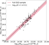 |
Fig. 7. Comparison of the total masses inside the Planck-ESZ sample between XMM-Newton and Chandra. |
 (15)
(15)
with an intrinsic scatter σi = 15.2 ± 1.3%.
We show that we are fully compatible with a mass-independent mass calibration bias. We still however observe an offset, with the masses from XMM-Newton being globally lower than the Chandra masses. This result had already been shown previously (see Appendix D of Schellenberger et al. 2015). This offset is however well accounted for by the 10% uncertainty we allow in the K prior in the majority of the sample. We do, however, point out that this comparison has been carried out only on the total masses, while our study is focused on the gas mass fraction. To be able to fully rule out possible biases from instrumental effects we would need to compare the gas mass fractions obtained from both observations rather than the total masses. Unfortunately as we do not have access to the gas masses from the Chandra observations, we can only assume that the compatibility we see for Mtot stays true for fgas. This assumption is sensible, as we have
 (16)
(16)
As it happens, the discrepancy between Chandra and XMM-Newton mass measurements originates mainly from the calibration of the temperature profiles (Schellenberger et al. 2015). As these profiles are not used in the computation of the gas masses and as the R500 used in both studies are compatible, is it reasonable to assume Mgas, Chandra/Mgas,XMM-Newton ∼ 1. We thus argue that the compatibility that we see between Chandra and XMM-Newton total mass measurements holds true for the gas fractions. We therefore assume that if calibration biases are affecting our study, they have only minor effects on our results.
5.1.2. Other contributions to the evolution of fgas
In this work, we consider the evolution of the gas fraction as a probe for the evolution of the hydrostatic mass bias, as well as a cosmological probe. As discussed in Sect. 2 and shown in Eq. (6) however, several physical and instrumental effects may vary with mass and redshift and play a role in the evolution of fgas.
The depletion factor Υ is fully degenerated with the hydrostatic mass bias, both regarding its value and its evolution with mass and redshift. As such, we need a robust prior on this parameter to be able to disentangle its effects on the fgas measurements from those of the bias. Following Planelles et al. (2013), here we considered a depletion at R500Υ = 0.85 ± 0.03, with no evolution with mass nor redshift. This value is lower than the value of Υ = 0.94 ± 0.03 from Eckert et al. (2019), however the use of different priors on the mean value of the depletion only affects the results on B0, and does not change the results on the mass and redshift evolution of the bias, as we show in Appendix C. Furthermore, the latter study shows no evolution of the depletion with mass or redshift. Henden et al. (2020) found a depletion Υ ∼ 0.8 in the clusters of the FABLE simulations, this time again with no clear trend with mass and redshift for clusters with M500 > 3 × 10¹⁴ M⊙, compatible with the prior assumed in this work. We however stress once again that both parameters are heavily degenerated and that a shift in the value of Υ will produce a similar shift in the predicted value of B0. As B0 and Ωb/Ωm are also degenerated, a shift in the value of Υ might also produce a shift in the predicted value of Ωb/Ωm. However, this has no effect on our values of α and β, nor on our constraints on other cosmological parameters.
In addition, a deviation from self-similarity due to baryonic physics may cause the Mtot − Mgas relation to be mass- and redshift-dependent. In Lovisari et al. (2020a), deviations from self-similarity of the ESZ cluster sample are studied. In particular, the redshift evolution of the relation is compatible with 0, in agreement with the self-similar prediction. On the other hand, the slope of the relation (i.e. its mass evolution), which we call γ departs from the self similar prediction by more than 4σ, with γ = 0.802 ± 0.049. This result however was obtained on the hydrostatic masses computed from the X-ray observations and, thus, the fitted relation is MHE − Mgas. We show in Appendix B that the observed evolution of fgas with mass is, consequently, most likely due to a combination of an evolution of the bias and a deviation of the true Mtot − Mgas relation from self-similarity. However, we cannot disentangle the two effects and acknowledge that assuming or not self-similarity may lead to changes in the value of the mass evolution of the bias (see e.g., Eckert et al. 2016 or Truong et al. 2018).
The calibration bias, K, may evolve with cluster mass. We show in Sect. 5.1.1 that when comparing Chandra and XMM-Newton masses such an evolution should be small. For this reason, any possible impact is accounted for by our prior on K.
The stellar fraction may also vary both with mass and with redshift (see e.g., Lin et al. 2012 or Henden et al. 2020). The mean value of this parameter being negligible, such an evolution only has a minor impact on our our results and we can consider it constant in our analysis, following the prior from Eckert et al. (2019).
Thus, the only two possible remaining contributions to the evolution of fgas are the hydrostatic bias, which can evolve with mass and redshift, and the cosmology, inducing a redshift evolution on the part of the gas fraction. Following our motivated choice of priors on both bias and cosmological parameters in the two parts of the analysis, we conclude that the only effect able to induce a mass and redshift evolution of fgas is the hydrostatic mass bias.
5.1.3. Role of the parametrization
In the previous work Wicker et al. (2022), we investigated the evolution of B with redshift, using a linear parametrization for the evolution of the bias,
 (17)
(17)
instead of a power law. Here, we compare the results given by this choice of parametrization to the results we got for a power law model. In this comparison of the linear case with the power law case we focus on the redshift dependence, as we did not find strong evidence for a mass evolution of the bias in the majority of our samples. We show in Figs. 8 and 9 and in Table 4 that the results are qualitatively consistent between the power law and linear descriptions. Indeed, in both cases, when considering the VB + Ωm scenario, we observe a strong sample dependence of the results. As a matter of fact, we show in Fig. 8 that the LowMz clusters strongly favor a non-zero slope, namely,  . On the high end of the mass-redshift plane, we find results that are consistent with the power law case and that are also compatible with no redshift evolution of B, as we find B1 = −0.095 ± 0.14. Our estimates of B0 are also consistent between the power law case and the linear case for each subsample respectively, as we find
  ,
,  and B0,full = 0.839 ± 0.046.
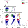 |
Fig. 8. 1D and 2D posteriors obtained when comparing the CB, VB and VB + Ωm scenarios with a linear parametrization. The contours mark the 68% and 95% c.l. and the gray dashed lines highlight reference values for (B1, Ωb/Ωm, Ωm)=(0, 0.156, 0.315). The orange bands mark the Planck Collaboration VI (2020) values for Ωb/Ωm and Ωm at 2σ c.l. |
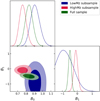 |
Fig. 9. 1D and 2D posteriors obtained when comparing the bias parameters derived for the three samples, when considering a linear evolution of the bias. The contours mark the 68% and 95% c.l. |
Constraints obtained on bias and cosmological parameters, when assuming a linear parametrization.
When studying the VB scenario, we still observe the strong degeneracy between the term accounting for the redshift evolution of B (here, B1) and Ωm. This explains why we again obtained aberrant values of Ωm when considering the CB scenario. This compatibility between the qualitative results given by both parametrizations would hint at the fact that our results are not dominated by our choice of model for the bias evolution.
5.2. Comparison with other studies
5.2.1. Mass and redshift trends of the bias
In this work, we show a strong sample dependence of our sampled results on different mass and redshift variations of the bias depending on the mass and redshift range of the subsample. We show that for low redshift and low mass clusters, the bias tends to stay constant with mass, while it increases toward higher redshift. The reverse behavior is observed in the case of high masses and high redshift clusters, with a bias that is constant with redshift but slightly increasing with the mass of the objects. This sample dependence had already been noted in Salvati et al. (2019), where the authors used tSZ number counts on the cosmology sample of the PSZ2 catalog Planck Collaboration XXIV (2016). The authors indeed noted a non-zero trend of the bias with redshift when considering their complete sample, which disappeared when considering only the clusters above z = 0.2. We note, however, that the compatibility of our results with that study regarding the mass and redshift trends depends on the considered subsample of clusters. We observe the same behavior regarding the value of the constant term of the bias B0, with compatible results for the high redshift clusters but incompatible ones when considering the full sample. We might argue that these differences come from different choices of priors in the two studies. Indeed, when investigating sample dependencies we did not assume any prior on the bias parameters and we considered priors on cosmology, whereas Salvati et al. (2019) assumed a prior on the total value of the bias and let their cosmological parameters remain free. However, this might not have such a strong impact, since in the first part in the analysis, we let the cosmological parameters free and we put a prior on the total value of the bias; in our results we do not see significant deviations in the value of B0 between the two cases. These differences are actually most probably due to differences between the clusters considered in the two studies, as the clusters from the ESZ sample have globally higher mass at an equivalent redshift than the PSZ2Cosmo sample considered in their study, as we show in Fig. 10. If anything, this could be yet another indication of the strong sample dependence in the results we present here.
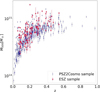 |
Fig. 10. Comparison between the PSZ2Cosmo sample used in Salvati et al. (2019) and the Planck-ESZ sample. |
Our results are nonetheless consistent with other weak lensing studies, which include Weighing the Giants (WtG, von der Linden et al. 2014) or CCCP (Hoekstra et al. 2015), displaying a mild decreasing trend in mass for B when considering high redshift (zWtG = 0.31, zCCCP = 0.246) and high mass (M500, WtG = 13.58 × 10¹⁴ M⊙, M500, CCCP = 10.38 × 10¹⁴ M⊙) clusters. More recent works such as the X-ray study X-COP (Eckert et al. 2019) also seem to show a possible mass-dependent bias, with a decreasing trend of B. The weak-lensing studies LOCUSS (Smith et al. 2016) and COMALIT (Sereno & Ettori 2017) both find decreasing trends of B with redshift, in agreement with this work, for clusters in the mass and redshift range of our sample (zLoCuSS = 0.22, MLoCuSS = 6.8 × 10¹⁴ M⊙).
On a side note, our results regarding the amplitude, B0, are also compatible with Lovisari et al. (2020b), where the authors measured the ratio of hydrostatic to weak lensing mass MHE/MWL inside the Planck-ESZ sample. The authors found a ratio (MHE/MWL)ESZ = 0.74 ± 0.06, which is in agreement with our amplitude B0, ESZ = 0.840 ± 0.095.
5.2.2. Discussing the choice of a sample at R500
In this work, we focus on gas fractions taken at R500, which is larger than most works using fgas as a cosmological probe, carried out at R2500. The choice of R2500 is generally motivated by the low scatter of the gas fraction data around those radii (see Mantz et al. 2014 and references therein), allowing for more precise cosmological constraints. The scatter fgas in data is larger at R500, however, this inconvenient is balanced by the stability of the depletion factor Υ at this radius. Indeed, as shown by the hydrodynamical simulations from Planelles et al. (2013), the value of Υ does not vary much with the radius when it is measured around R500. This reduces the possibility of a biased estimation of the depletion due to incorrect determinations of R500. On the other hand Υ starts to decrease in the vicinity of R2500. As a consequence, if the radius is not properly measured, (e.g., due to erroneous estimations of the density contrast), the estimation of the depletion will be biased. Our purpose in this study being to constrain the hydrostatic mass bias and its evolution, we need a robust prior on the depletion factor, due to the degeneracy between Υ and B. A bias in the value of the depletion due to an incorrectly measured radius would then impact our results on the mean value and evolution of B.
5.3. Discussing the tension on the bias value
Finally, we highlight that the value of B0 = 0.840 ± 0.095 we found for the full sample is in agreement with a collection of other studies, including the aforementioned weak-lensing and X-ray studies, as well as with works from hydrodynamical simulations, as shows in Fig. 11. The works shown in Fig. 11 are those for which the bias is known at R500 with a central value and error bars, where the mean mass and redshift of the samples are available. We show, however, that this value is incompatible with the values B0 = 0.62 ± 0.03 from Planck Collaboration VI (2020), or B0 ≲ 0.67 from Salvati et al. (2018), which are needed to reconcile local measurements of the bias with the combination of CMB and tSZ number counts measurements. Indeed, as we show in Fig. 11, the tension is alleviated only for the highest redshifts and, more particularly for the highest masses, for clusters with M ≳ 1015 M⊙.
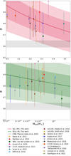 |
Fig. 11. Comparison of our value of the mass bias depending on mass and redshift with other works in X-ray, weak lensing, and hydrodynamical simulations. In both panels, the shaded areas mark the 1 and 2σ confidence levels and the gray band marks the value preferred by CMB observations of B = 0.62 ± 0.003. The half-filled circles are hydrodynamical simulation works. Other points represent works based on observations. Top: value of the bias depending on redshift, computed for the mean mass of our sample. Bottom: value of the bias depending on mass, computed at the mean redshift of our sample. References: Rasia et al. (2012), Mahdavi et al. (2013), von der Linden et al. (2014), Gruen et al. (2014), Hoekstra et al. (2015), Israel et al. (2015), Biffi et al. (2016), Okabe & Smith (2016), Smith et al. (2016), Sereno et al. (2017), Gupta et al. (2017), Jimeno et al. (2018), Medezinski et al. (2018), Eckert et al. (2019), Salvati et al. (2019), Herbonnet et al. (2020), Lovisari et al. (2020b), Planck Collaboration VI (2020), Gianfagna et al. (2021). |
Similarly the X-COP study (Eckert et al. 2019) shows that assuming a bias of B = 0.58 ± 0.04 from Planck Collaboration XXIV (2016) results in gas fractions that are way lower than expected, as they find a median gas fraction of their sample fgas, B = 0.58 = 0.108 ± 0.006. This would imply that the galaxy clusters from their sample are missing about a third of their gas. A low value for the bias thus seems highly unlikely given its implications fir the gas content of galaxy clusters.
We show a similar result in this work. Indeed, from Eq. (6), it is possible to compute the expected universal baryon fraction for a certain value of the bias, namely:
 (18)
(18)
meaning Ωb/Ωm ∝ B. When assuming a low value of the bias B = 0.62 ± 0.03 from Planck Collaboration VI (2020), we show that the derived baryon fraction becomes Ωb/Ωm = 0.108 ± 0.018, which is incompatible with the value of the baryon fraction derived from the CMB, Ωb/Ωm = 0.156 ± 0.003 (Planck Collaboration VI 2020), as we show in Fig. 12. Assuming a low value of the bias would then imply that the Universe hosts roughly 20% less baryons than expected. We thus argue that a value of the bias B = 0.62 ± 0.03 seems highly unlikely provided our gas fraction data.
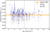 |
Fig. 12. Comparison of the expected baryon fraction Ωb/Ωm between the bias we derived in the VB + Ωm scenario and B = 0.62 from (Planck Collaboration VI 2020). |
6. Conclusion
We measured the gas mass fraction of galaxy clusters at R500 and used it to constrain a possible mass and redshift evolution of the hydrostatic mass bias. To do so, we compared the cosmological constraints we obtained when assuming a varying bias to those we obtained when assuming a constant B. We show that assuming a redshift evolution seems necessary when performing a cosmological analysis using fgas data at R500. Indeed we show a significant degeneracy between the redshift dependence of the bias β and the matter density Ωm. This degeneracy implies that high and close to zero β push the matter density to higher values. As a consequence, assuming a constant bias implies Ωm > 0.860, which is aberrant. Forcing Ωm to have sensible values by imposing a Planck Collaboration VI (2020) prior in turns induces β = −0.64 ± 0.17, in a 3.8σ tension with 0.
We show, however, that these results are strongly dependent on the considered sample. Indeed for the least massive clusters of our sample at the lowest redshifts, we show an important decreasing trend of B with redshift and no trend with mass, with the set  . On the other hand, for the most massive clusters at highest redshifts, we observe no variation with redshift but we see that a decreasing evolution with mass is favored, with (α, β)=(−0.149 ± 0.058, −0.08 ± 0.23). When we consider the full sample, the results we obtain lie between the two extremes, largely favoring a decreasing trend of B with redshift, yet remaining compatible with no mass trend of the bias as we obtain (α, β)=(−0.057 ± 0.038, −0.64 ± 0.18). We recall, however, that other selection effects might affect our results as the clusters at the highest redshifts are also generally the most massive. In addition, deviations from self-similarity may lead to changes in the value of the mass evolution of the bias.
In order to identify and rule out different sources of systematic effects in our study, we looked at the possibility of being subject to instrumental calibration effects. Using mass measurements of the galaxy clusters in our sample both from Chandra and XMM-Newton, we find no evidence of a bias that would significantly change our results. In this study, we assumed a power-law description for the evolution of the bias. We look at the effect of this choice of parametrization by comparing our results to those we obtain when assuming a linear evolution of B with redshift. We find no major difference with the power law case, as we still observe a strong degeneracy between the redshift evolution of B and Ωm, favoring an evolution of the bias with redshift when considering a Planck prior on Ωm. Furthermore, the sample dependence we observe for the power law case holds true when assuming a linear evolution of the bias.
Despite these results, we stress that our results remain compatible with a collection of X-ray, weak lensing, and hydrodynamical simulation works regarding the mean value of the bias, given our finding of B0 = 0.840 ± 0.095. This value remains, on the other hand, in tension with the value required from the combination of CMB observations and tSZ cluster counts to alleviate the tension on σ8.
Finally, we recall that this work is focused on gas fractions taken at R500, with a goal to obtain constraints on two cosmological parameters, the universal baryon fraction, Ωb/Ωm, and the matter density of the Universe, Ωm, which are the two parameters mainly probed by fgas. We thus argue that the gas fraction can be used to set constraints on the cosmological model, albeit provided that one properly models the gas effects taking place inside clusters and provided that fgas is used in combination with other probes.
Acknowledgments
The authors thank the anonymous referee for their helpful comments and discussion. They also acknowledge the fruitful discussions and comments from Lorenzo Lovisari, Stefano Ettori, Hideki Tanimura, Daniela Galárraga-Espinosa, Edouard Lecoq, Joseph Kuruvilla and Celine Gouin. The authors also thank the organisers and participants of the 2021 edition of the “Observing the mm Universe with the NIKA2 Camera” conference for their useful comments and discussions. RW acknowledges financial support from the Ecole Doctorale d’Astronomie et d’Astrophysique d’Ile-de-France (ED AAIF). This research has made use of the SZ-Cluster Database operated by the Integrated Data and Operation Center (IDOC) at the Institut d’Astrophysique Spatiale (IAS) under contract with CNES and CNRS. This project was carried out using the Python libraries matplotlib (Hunter 2007), numpy (Harris et al. 2020), astropy (Astropy Collaboration 2013, 2018) and pandas (Reback et al. 2021). It also made use of the Python library for MCMC sampling emcee (Foreman-Mackey et al. 2013), and of the getdist (Lewis 2019) package to read posterior distributions.
References
- Allen, S. W., Schmidt, R. W., & Fabian, A. C. 2002, MNRAS, 334, L11 [NASA ADS] [CrossRef] [Google Scholar]
- Allen, S. W., Rapetti, D. A., Schmidt, R. W., et al. 2008, MNRAS, 383, 879 [Google Scholar]
- Allen, S. W., Evrard, A. E., & Mantz, A. B. 2011, ARA&A, 49, 409 [Google Scholar]
- Andrade-Santos, F., Pratt, G. W., Melin, J.-B., et al. 2021, ApJ, 914, 58 [NASA ADS] [CrossRef] [Google Scholar]
- Astropy Collaboration (Robitaille, T. P., et al.) 2013, A&A, 558, A33 [NASA ADS] [CrossRef] [EDP Sciences] [Google Scholar]
- Astropy Collaboration (Price-Whelan, A. M., et al.) 2018, AJ, 156, 123 [Google Scholar]
- Balmés, I., Rasera, Y., Corasaniti, P.-S., & Alimi, J.-M. 2013, MNRAS, 437, 2328 [Google Scholar]
- Battaglia, N., Bond, J. R., Pfrommer, C., & Sievers, J. L. 2012, ApJ, 758, 74 [NASA ADS] [CrossRef] [Google Scholar]
- Battaglia, N., Bond, J. R., Pfrommer, C., & Sievers, J. L. 2013, ApJ, 777, 123 [NASA ADS] [CrossRef] [Google Scholar]
- Bennett, J. S., & Sijacki, D. 2022, MNRAS, 514, 313 [CrossRef] [Google Scholar]
- Biffi, V., Borgani, S., Murante, G., et al. 2016, ApJ, 827, 112 [NASA ADS] [CrossRef] [Google Scholar]
- Borgani, S., & Kravtsov, A. 2011, Adv. Sci. Lett., 4, 204 [Google Scholar]
- Crain, R. A., Eke, V. R., Frenk, C. S., et al. 2007, MNRAS, 377, 41 [NASA ADS] [CrossRef] [Google Scholar]
- Cui, W., Knebe, A., Yepes, G., et al. 2018, MNRAS, 480, 2898 [Google Scholar]
- Eckert, D., Ettori, S., Coupon, J., et al. 2016, A&A, 592, A12 [NASA ADS] [CrossRef] [EDP Sciences] [Google Scholar]
- Eckert, D., Ghirardini, V., Ettori, S., et al. 2019, A&A, 621, A40 [NASA ADS] [CrossRef] [EDP Sciences] [Google Scholar]
- Eke, V. R., Navarro, J. F., & Frenk, C. S. 1998, ApJ, 503, 569 [NASA ADS] [CrossRef] [Google Scholar]
- Foreman-Mackey, D., Hogg, D. W., Lang, D., & Goodman, J. 2013, PASP, 125, 306 [Google Scholar]
- Galárraga-Espinosa, D., Langer, M., & Aghanim, N. 2022, A&A, 661, A115 [NASA ADS] [CrossRef] [EDP Sciences] [Google Scholar]
- Gianfagna, G., De Petris, M., Yepes, G., et al. 2021, MNRAS, 502, 5115 [NASA ADS] [CrossRef] [Google Scholar]
- Gouin, C., Gallo, S., & Aghanim, N. 2022, A&A, 664, A198 [NASA ADS] [CrossRef] [EDP Sciences] [Google Scholar]
- Gruen, D., Seitz, S., Brimioulle, F., et al. 2014, MNRAS, 442, 1507 [CrossRef] [Google Scholar]
- Gupta, N., Saro, A., Mohr, J. J., Dolag, K., & Liu, J. 2017, MNRAS, 469, 3069 [Google Scholar]
- Harris, C. R., Millman, K. J., van der Walt, S. J., et al. 2020, Nature, 585, 357 [NASA ADS] [CrossRef] [Google Scholar]
- Henden, N. A., Puchwein, E., & Sijacki, D. 2020, MNRAS, 498, 2114 [Google Scholar]
- Herbonnet, R., Sifón, C., Hoekstra, H., et al. 2020, MNRAS, 497, 4684 [NASA ADS] [CrossRef] [Google Scholar]
- Hoekstra, H., Mahdavi, A., Babul, A., & Bildfell, C. 2012, MNRAS, 427, 1298 [NASA ADS] [CrossRef] [Google Scholar]
- Hoekstra, H., Herbonnet, R., Muzzin, A., et al. 2015, MNRAS, 449, 685 [NASA ADS] [CrossRef] [Google Scholar]
- Holanda, R. F. L., Pordeus-da-Silva, G., & Pereira, S. H. 2020, JCAP, 2020, 053 [CrossRef] [Google Scholar]
- Hunter, J. D. 2007, Comput. Sci. Eng., 9, 90 [NASA ADS] [CrossRef] [Google Scholar]
- Israel, H., Schellenberger, G., Nevalainen, J., Massey, R., & Reiprich, T. H. 2015, MNRAS, 448, 814 [NASA ADS] [CrossRef] [Google Scholar]
- Jimeno, P., Diego, J. M., Broadhurst, T., De Martino, I., & Lazkoz, R. 2018, MNRAS, 478, 638 [NASA ADS] [CrossRef] [Google Scholar]
- Kravtsov, A. V., & Borgani, S. 2012, ARA&A, 50, 353 [Google Scholar]
- Kravtsov, A. V., Nagai, D., & Vikhlinin, A. A. 2005, ApJ, 625, 588 [Google Scholar]
- Lau, E. T., Kravtsov, A. V., & Nagai, D. 2009, ApJ, 705, 1129 [NASA ADS] [CrossRef] [Google Scholar]
- Lewis, A. 2019, ArXiv e-prints [arXiv:1910.13970] [Google Scholar]
- Lin, Y.-T., Stanford, S. A., Eisenhardt, P. R. M., et al. 2012, ApJ, 745, L3 [Google Scholar]
- Lovisari, L., Ettori, S., Sereno, M., et al. 2020a, A&A, 644, A78 [NASA ADS] [CrossRef] [EDP Sciences] [Google Scholar]
- Lovisari, L., Schellenberger, G., Sereno, M., et al. 2020b, ApJ, 892, 102 [Google Scholar]
- Mahdavi, A., Hoekstra, H., Babul, A., et al. 2013, ApJ, 767, 116 [NASA ADS] [CrossRef] [Google Scholar]
- Mantz, A. B., Allen, S. W., Morris, R. G., et al. 2014, MNRAS, 440, 2077 [NASA ADS] [CrossRef] [Google Scholar]
- Mantz, A. B., Morris, R. G., Allen, S. W., et al. 2022, MNRAS, 510, 131 [Google Scholar]
- McCarthy, I. G., Babul, A., Holder, G. P., & Balogh, M. L. 2003a, ApJ, 591, 515 [NASA ADS] [CrossRef] [Google Scholar]
- McCarthy, I. G., Holder, G. P., Babul, A., & Balogh, M. L. 2003b, ApJ, 591, 526 [NASA ADS] [CrossRef] [Google Scholar]
- McCarthy, I. G., Schaye, J., Bird, S., & Le Brun, A. M. C. 2017, MNRAS, 465, 2936 [Google Scholar]
- Medezinski, E., Battaglia, N., Umetsu, K., et al. 2018, PASJ, 70, S28 [NASA ADS] [Google Scholar]
- Nelson, K., Lau, E. T., & Nagai, D. 2014, ApJ, 792, 25 [NASA ADS] [CrossRef] [Google Scholar]
- Okabe, N., & Smith, G. P. 2016, MNRAS, 461, 3794 [Google Scholar]
- Planck Collaboration VIII. 2011, A&A, 536, A8 [NASA ADS] [CrossRef] [EDP Sciences] [Google Scholar]
- Planck Collaboration XX. 2014, A&A, 571, A20 [NASA ADS] [CrossRef] [EDP Sciences] [Google Scholar]
- Planck Collaboration XXIV. 2016, A&A, 594, A24 [NASA ADS] [CrossRef] [EDP Sciences] [Google Scholar]
- Planck Collaboration VI. 2020, A&A, 641, A6 [NASA ADS] [CrossRef] [EDP Sciences] [Google Scholar]
- Planelles, S., Borgani, S., Dolag, K., et al. 2013, MNRAS, 431, 1487 [Google Scholar]
- Poole, G. B., Babul, A., McCarthy, I. G., et al. 2007, MNRAS, 380, 437 [NASA ADS] [CrossRef] [Google Scholar]
- Pratt, G. W., Arnaud, M., Biviano, A., et al. 2019, Space Sci. Rev., 215, 25 [Google Scholar]
- Rasia, E., Ettori, S., Moscardini, L., et al. 2006, MNRAS, 369, 2013 [CrossRef] [Google Scholar]
- Rasia, E., Meneghetti, M., Martino, R., et al. 2012, New J. Phys., 14, 055018 [Google Scholar]
- Reback, J., McKinney, W., jbrockmendel, et al. 2021, https://doi.org/10.5281/zenodo.4681666 [Google Scholar]
- Ruan, J. J., Quinn, T. R., & Babul, A. 2013, MNRAS, 432, 3508 [NASA ADS] [CrossRef] [Google Scholar]
- Sakr, Z., Ilić, S., Blanchard, A., Bittar, J., & Farah, W. 2018, A&A, 620, A78 [NASA ADS] [CrossRef] [EDP Sciences] [Google Scholar]
- Salvati, L., Douspis, M., & Aghanim, N. 2018, A&A, 614, A13 [NASA ADS] [CrossRef] [EDP Sciences] [Google Scholar]
- Salvati, L., Douspis, M., Ritz, A., Aghanim, N., & Babul, A. 2019, A&A, 626, A27 [NASA ADS] [CrossRef] [EDP Sciences] [Google Scholar]
- Sarazin, C. L. 1988, X-ray Emission from Clusters of Galaxies (Cambridge: Cambridge University Press) [Google Scholar]
- Schellenberger, G., Reiprich, T. H., Lovisari, L., Nevalainen, J., & David, L. 2015, A&A, 575, A30 [NASA ADS] [CrossRef] [EDP Sciences] [Google Scholar]
- Sembolini, F., Yepes, G., Pearce, F. R., et al. 2016, MNRAS, 457, 4063 [Google Scholar]
- Sereno, M., & Ettori, S. 2017, MNRAS, 468, 3322 [CrossRef] [Google Scholar]
- Sereno, M., Covone, G., Izzo, L., et al. 2017, MNRAS, 472, 1946 [Google Scholar]
- Shi, X., Komatsu, E., Nelson, K., & Nagai, D. 2015, MNRAS, 448, 1020 [NASA ADS] [CrossRef] [Google Scholar]
- Smith, G. P., Mazzotta, P., Okabe, N., et al. 2016, MNRAS, 456, L74 [Google Scholar]
- Sunyaev, R. A., & Zeldovich, Y. B. 1972, Comm. Astrophys. Space Phys., 4, 173 [Google Scholar]
- Truong, N., Rasia, E., Mazzotta, P., et al. 2018, MNRAS, 474, 4089 [NASA ADS] [CrossRef] [Google Scholar]
- Vazza, F., Brunetti, G., Kritsuk, A., et al. 2009, A&A, 504, 33 [NASA ADS] [CrossRef] [EDP Sciences] [Google Scholar]
- von der Linden, A., Mantz, A., Allen, S. W., et al. 2014, MNRAS, 443, 1973 [NASA ADS] [CrossRef] [Google Scholar]
- White, S. D. M., Navarro, J. F., Evrard, A. E., & Frenk, C. S. 1993, Nature, 366, 429 [Google Scholar]
- Wicker, R., Douspis, M., Salvati, L., & Aghanim, N. 2022, Eur. Phys. J. Web Conf., 257, 00046 [CrossRef] [EDP Sciences] [Google Scholar]
Appendix A: Cluster sample
The redshifts, gas masses, total masses, and gas mass fractions within R500 of the clusters we used for this study are given in Table A.1. The redshifts and gas and total masses for the clusters were taken from Lovisari et al. (2020a). We computed the gas fractions from these masses.
First four of the 120 clusters we used in this study, from the Planck-ESZ sample.
Appendix B: Effect of non self-similarity
The scaling relations between two quantities (X, Y) from Lovisari et al. (2020a) are fitted using the following generic form:
 (B.1)
(B.1)
with
where C1 and C2 are pivot points, ϵ is the normalisation, γ the slope of the relation, δ its evolution with redshift, σ the intrinsic scatter in the two variables and Fz = E(z)/E(z)ref (Lovisari et al. 2020a). As a result, when we focus on the MHE − Mgas relation, we have the following expression (we ignore σ for simplicity as they only represent a scatter, i.e. an uncertainty, around a mean value):
 (B.2)
(B.2)
 (B.3)
(B.3)
In particular, the value for δ measured by Lovisari et al. (2020a) is δ = −0.317 ± 0.307. Even if this value is consistent with 0 within 1σ, the error bars encompass a large range of values, up to δ = −0.6, which represents a strong evolution. We test therefore the impact of having δ ≠ 0. We find here that this assumption does not affect our results, as the factor  does not deviate from 1 when we are close to the reference cosmology. In our analysis, the cosmological constraints we find are always in agreement with a Planck Collaboration VI (2020) cosmology within 1σ (see Table 2). When using this cosmology in our redshift range, we always remain compatible with
  within 1σ, with less than 1% of deviation. This term can thus be ignored in the rest of the analysis, and we are left with the following relation:
 (B.4)
(B.4)
For displaying purposes we set:
We obtain the following expression, as MHE = B(M, z)⋅Mtot:
 (B.5)
(B.5)
We remind that throughout the paper we assumed a power law evolution of the bias  . We thus have the following relation:
 (B.6)
(B.6)
 (B.7)
(B.7)
and the fitted Mtot − Mgas scaling relation can be summed up as follows:
 (B.8)
(B.8)
In the paper, we find an evolution of the gas fraction  for the full sample. There are several possibilities to explain this result when accounting for deviations of the Mtot − Mgas relation from self-similarity:
-
The self-similar hypothesis predicts a linear and redshift independent relation between the total mass and the gas mass, i.e. α + 1 = γ and β(1 − γ)=0. In this description, all the mass and redshift evolution of the gas fraction comes from the bias. From Lovisari et al. (2020a) we have γ = 0.802 ± 0.049. This means that in the self-similar case, we should obtain α = −0.198 ± 0.049 i.e.
 , which is in tension with our measured value at 2.9σ. In addition, from our measured value of β = −0.64 ± 0.17, we find β(1 − γ)= − 0.13 ± 0.05, in tension with 0 at 2.6σ. This hints at the fact that the mass and redshift evolution of fgas can not be accounted for solely by an evolution of the bias. Instead, a deviation from self-similarity of the Mtot − Mgas relation is necessary to explain our results.
 -
As we show a deviation of the Mtot − Mgas relation from self-similarity, one may wonder whether this effect may totally mimic the effect of a mass evolution of the bias. This is however not the case. Indeed, if we set a constant bias α = β = 0, then
 (found with the full sample), leading to γ = 0.946 ± 0.034, in tension at 4σ the with the value found by Lovisari et al. (2020a) of γ = 0.802 ± 0.049. Furthermore, putting β = 0 leads to
  , i.e. a redshift independent gas fraction. This is however not what we observe.
We thus show that the dependence of fgas on mass and redshift cannot be due to deviations from self-similarity or to an evolution of the bias alone. Instead, it can only be explained by a combination of the two effects.
Appendix C: Effect of the prior on the depletion Υ0
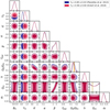 |
Fig. C.1. MCMC results for a 10% shift of the depletion factor in our analysis in the VB scenario. We note that in this case, we assume a prior on the total value of the bias. |
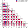 |
Fig. C.2. MCMC results for a 10% shift of the depletion factor in our analysis in the VB scenario, without any prior on the total value of the bias. |
Constraints on the model parameters in the VB scenario after a 10% shift of the depletion factor.
In order to properly assess the effect of the depletion factor on our conclusions, we performed runs of the VB scenario when considering two different values of the depletion, the one we assumed throughout the paper Υ0 = 0.85 ± 0.03 from Planelles et al. (2013) and Υ0 = 0.94 ± 0.04 from Eckert et al. (2019).
When we apply a 10% shift in the value of the depletion, we do not observe a significant shift in the value of the other parameters, as we show in Figure C.1 and Table C.1. We however acknowledge that this result is due to the presence of a prior on the total value of the bias, which we assume in the first part of the analysis. To try to quantify the impact of this prior, we leave the bias fully free in second MCMC runs. We show the results in Figure C.2 Table C.1. Similarly to the previous case, we do not observe a particular shift of the constraints from a shift of the depletion, mostly because the posterior distribution are extremely wide. In particular, we do not find a degeneracy between Υ and other parameters, including B0 or cosmological parameters. We thus claim that although the depletion factor is indeed a strong systematic in our analysis, we address it properly.
All Tables
Constraints obtained on bias and cosmological parameters in the CB, VB and VB + Ωm scenarios.
Constraints obtained on bias and cosmological parameters, when assuming a linear parametrization.
First four of the 120 clusters we used in this study, from the Planck-ESZ sample.
Constraints on the model parameters in the VB scenario after a 10% shift of the depletion factor.
All Figures
|
Fig. 1. Gas mass fraction of Planck-ESZ clusters with respect to redshift (top) and with respect to cluster mass (bottom). The yellow bands in both plots mark the Planck Collaboration VI (2020) value of Ωb/Ωm = 0.156 ± 0.003. |
| In the text | |
|
Fig. 2. Binned mass-redshift plane of the Planck-ESZ sample. Inside each bin we compute the mean value of fgas. We show the number of clusters included in each bin and mark the delimitation of each subsample. |
| In the text | |
|
Fig. 3. 1D and 2D posterior distributions for the CB, VB, and VB + Ωm scenarios. The contours mark the 68% and 95% confidence level (c.l.). The gray dashed lines highlight reference values for (α, β, Ωb/Ωm, Ωm)=(0, 0, 0.156, 0.315). The orange bands mark the Planck Collaboration VI (2020) values for Ωb/Ωm and Ωm at 2σ c.l. |
| In the text | |
|
Fig. 4. Posterior distributions showing the degeneracy between β and Ωm. The contours mark the 68% and 95% c.l. The gray dashed lines highlight reference values for (β, Ωm)=(0, 0.315). The orange band marks the Planck Collaboration VI (2020) value for Ωm at 2σ c.l. |
| In the text | |
|
Fig. 5. 1D and 2D posterior distributions for the bias parameters in the three mass- and redshift-selected samples. The levels of the contours mark the 68% and 95% confidence levels. Gray dashed lines mark the reference values (α, β)=(0, 0). |
| In the text | |
|
Fig. 6. Fits obtained from our analysis, for the different mass- and redshift-selected samples. The results in the top two panels are represented with respect to redshift at constant mass (respectively minimal and maximal masses of the full sample), while the bottom two panels are the results presented with respect to mass, at a fixed redshift (respectively minimal and maximal redshifts of the full sample). The shaded areas around the curves mark the 68% and 95% confidence levels. The blue dashed line marks the reference value Ωb/Ωm = 0.156. |
| In the text | |
|
Fig. 7. Comparison of the total masses inside the Planck-ESZ sample between XMM-Newton and Chandra. |
| In the text | |
|
Fig. 8. 1D and 2D posteriors obtained when comparing the CB, VB and VB + Ωm scenarios with a linear parametrization. The contours mark the 68% and 95% c.l. and the gray dashed lines highlight reference values for (B1, Ωb/Ωm, Ωm)=(0, 0.156, 0.315). The orange bands mark the Planck Collaboration VI (2020) values for Ωb/Ωm and Ωm at 2σ c.l. |
| In the text | |
|
Fig. 9. 1D and 2D posteriors obtained when comparing the bias parameters derived for the three samples, when considering a linear evolution of the bias. The contours mark the 68% and 95% c.l. |
| In the text | |
|
Fig. 10. Comparison between the PSZ2Cosmo sample used in Salvati et al. (2019) and the Planck-ESZ sample. |
| In the text | |
|
Fig. 11. Comparison of our value of the mass bias depending on mass and redshift with other works in X-ray, weak lensing, and hydrodynamical simulations. In both panels, the shaded areas mark the 1 and 2σ confidence levels and the gray band marks the value preferred by CMB observations of B = 0.62 ± 0.003. The half-filled circles are hydrodynamical simulation works. Other points represent works based on observations. Top: value of the bias depending on redshift, computed for the mean mass of our sample. Bottom: value of the bias depending on mass, computed at the mean redshift of our sample. References: Rasia et al. (2012), Mahdavi et al. (2013), von der Linden et al. (2014), Gruen et al. (2014), Hoekstra et al. (2015), Israel et al. (2015), Biffi et al. (2016), Okabe & Smith (2016), Smith et al. (2016), Sereno et al. (2017), Gupta et al. (2017), Jimeno et al. (2018), Medezinski et al. (2018), Eckert et al. (2019), Salvati et al. (2019), Herbonnet et al. (2020), Lovisari et al. (2020b), Planck Collaboration VI (2020), Gianfagna et al. (2021). |
| In the text | |
|
Fig. 12. Comparison of the expected baryon fraction Ωb/Ωm between the bias we derived in the VB + Ωm scenario and B = 0.62 from (Planck Collaboration VI 2020). |
| In the text | |
|
Fig. C.1. MCMC results for a 10% shift of the depletion factor in our analysis in the VB scenario. We note that in this case, we assume a prior on the total value of the bias. |
| In the text | |
|
Fig. C.2. MCMC results for a 10% shift of the depletion factor in our analysis in the VB scenario, without any prior on the total value of the bias. |
| In the text | |
Current usage metrics show cumulative count of Article Views (full-text article views including HTML views, PDF and ePub downloads, according to the available data) and Abstracts Views on Vision4Press platform.
Data correspond to usage on the plateform after 2015. The current usage metrics is available 48-96 hours after online publication and is updated daily on week days.
Initial download of the metrics may take a while.