| Issue |
A&A
Volume 709, May 2026
|
|
|---|---|---|
| Article Number | A72 | |
| Number of page(s) | 16 | |
| Section | Cosmology (including clusters of galaxies) | |
| DOI | https://doi.org/10.1051/0004-6361/202557423 | |
| Published online | 05 May 2026 | |
The SRG/eROSITA All-Sky Survey
Detection of shock-heated gas beyond the halo boundary into the accretion region
1
Max Planck Institute for Extraterrestrial Physics, Giessenbachstrasse 1, 85748, Garching, Germany
2
Department of Astronomy, University of Maryland, College Park, MD, 20742, USA
3
INAF, Osservatorio di Astrofisica e Scienza dello Spazio, via Piero Gobetti 93/3, I-40129, Bologna, Italy
4
Institute for Frontiers in Astronomy and Astrophysics, Beijing Normal University, Beijing, 102206, China
★ Corresponding author: This email address is being protected from spambots. You need JavaScript enabled to view it.
Received:
26
September
2025
Accepted:
2
March
2026
Abstract
The hot gas in the outskirts of galaxy cluster-sized halos, extending around and beyond the virial radius into nearby accretion regions, remains among one of the least explored baryon components of the large-scale cosmic structure. We present a stacking analysis of 680 galaxy clusters located in the western Galactic hemisphere, using data from the first two years of the Spectrum-Roentgen-Gamma/eROSITA All-Sky Survey. The stacked X-ray surface brightness profile reveals a statistically significant signal extending out to 2 × r200m (∼4.5 Mpc). The best-fit surface brightness profile is well described by a combination of terms describing orbiting and infalling gas, with a transition occurring around r200m. At this radius, the best-fit gas number density is 2.5 × 10⁻⁵ cm−3, corresponding to a baryon overdensity of 30. By integrating the gas density profile out to r200m, we inferred a gas fraction higher than the universal baryon fraction with the assumption of a typical halo concentration. However, correcting for possible clumping effects reduces the baryon fraction by more than 20%. Additionally, we examined the distribution of hot gas in massive clusters in the IllustrisTNG simulations, from the halo center to the accretion region. This analysis reveals differences in radial gas profiles depending on whether the direction points toward voids or toward nearby cosmic filaments. Beyond r200m, the density profile along the filament direction exceeds that along the void direction. This pattern aligns with the observed transition radius between the one-halo and two-halo terms, suggesting that r200m is the approximate radius marking the location at which cosmic filaments connect to galaxy clusters. Meanwhile, comparisons of the gas density and gas fraction profiles between the observation and the IllustrisTNG simulation suggest that the feedback processes in the stacking sample are more efficient at distributing gas to large radii than the IllustrisTNG model.
Key words: galaxies: clusters: general / galaxies: clusters: intracluster medium / large-scale structure of Universe / X-rays: galaxies: clusters
© The Authors 2026
 Open Access article, published by EDP Sciences, under the terms of the Creative Commons Attribution License (https://creativecommons.org/licenses/by/4.0), which permits unrestricted use, distribution, and reproduction in any medium, provided the original work is properly cited.
This article is published in open access under the Subscribe to Open model.
Open access funding provided by Max Planck Society.
1. Introduction
Galaxy clusters, the most massive collapsed dark matter halos in the Universe, are positioned at the nodes of the cosmic web. Galaxy clusters comprise T > 107 K hot baryonic gas as one sixth of their total mass and the remaining dark matter. While the gravitational potential is governed by dark matter, baryonic physics determines the properties of the hot gas. The cluster outskirts, here defined as the regions beyond r500c1, are of particular interest as they hold critical information about both the distribution of dark matter and the thermodynamic state of the gas.
The radial density profile in the outskirts is characterized by halo mass accretion, for which the behavior of dark matter differs from that of baryons due to their collisional and collisionless nature (Bertschinger 1985). In the case of collisionless dark matter, the infalling matter accumulates near the first apocenter of its orbit (e.g., Fillmore & Goldreich 1984; Bertschinger 1985; Adhikari et al. 2014). This leads to a phenomenon known as splashback, where the accreted matter causes a sharp decline in the outer density profile at radii around or beyond r200m. The exact location of this splashback radius is closely linked to the matter accretion rate (e.g., Diemer & Kravtsov 2014; Diemer et al. 2017a). On the other hand, infalling collisional gas forms accretion shocks2 (e.g., Bertschinger 1985; Ostriker & McKee 1988; Shi 2016), heating the cool intergalactic medium (IGM) to T ≳ 106 K and creating a turbulent atmosphere outside the splashback radius (Aung et al. 2021). In reality, the distribution and thermodynamic properties of shock-heated gas3 are more complex than suggested by the self-similar spherical collapse scenario, for example, because they are subject to nonthermal pressure support, infalling gas from cosmic filaments, merging, and kinetic feedback from the halo center. Figure 1 demonstrates the X-ray emission from the hot shock-heated gas in and around a massive halo from a numerical simulation. It shows that the shock-heated gas fills the vast space in the outskirts and beyond. At radii beyond r200m, the hot gas distribution is complicated by the presence of small halos falling onto the central halo. At even larger radii, the accretion shock confines the hot gas, and cosmic filaments connect the halo to the large-scale structure.
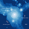 |
Fig. 1. Spatial distribution of the X-ray emission from the hot gas around a massive dark matter halo. The dashed circle indicates the size of r200m. At large radii, the halo is connected to and accreting smaller nearby halos from cosmic filaments. This map is produced using gas particles from a 20 × 20 × 20 Mpc3 box around the id=32 halo in the z = 0 snapshot of the TNG300-1 simulation (see Sect. 4 for the details of map creation). The central halo is in a mass M500c = 2.8 × 10¹⁴ M⊙ and an r200m of 2.5 Mpc. Short arrows mark the accretion shock, i.e., the boundary between shock-heated gas and the cool intergalactic medium. |
X-rays and the Sunyaev-Zeldovich (SZ) effect are the two key observational techniques for exploring the properties of hot gas in the outskirts (see Reiprich et al. 2013; Walker et al. 2019, for reviews). Due to the rapidly declining X-ray surface brightness and SZ Compton-y signal at large radii, most hot gas studies of the outskirts are limited to radii within r200c (e.g., Simionescu et al. 2011; Walker et al. 2013; Eckert et al. 2013; Planck Collaboration V 2013; Bulbul et al. 2016; Ghirardini et al. 2019; Mirakhor & Walker 2020; McCall et al. 2024). Beyond that radius, the gas clumping (Nagai & Lau 2011; Zhuravleva et al. 2013; Eckert et al. 2015; Angelinelli et al. 2021; Zhu et al. 2023), the connection between clusters and cosmic filaments (Rost et al. 2021; Gouin et al. 2022; Malavasi et al. 2020, 2023), and the location of the accretion shock (Lau et al. 2015; Baxter et al. 2021) are poorly constrained by individual pointing observations.
Recently, several stacking analyses of X-ray and SZ survey data demonstrate high signal-to-noise ratio (S/N) in the stacked profiles beyond r200c. In particular, Anbajagane et al. (2022, 2024) stacked Atacama Cosmology Telescope and South Pole Telescope SZ survey data and discovered a 6σ pressure deficit with respect to the best-fit model at ∼r200m. Lyskova et al. (2023, hereafter L23) stacked 38 Planck SZ selected clusters (Planck Collaboration XXVII 2016; CHEX-MATE Collaboration 2021) using the eastern Galactic hemisphere eROSITA All Sky Survey (eRASS) X-ray data, and obtained a gas density profile out to 3 × r500c.
For this work, we stacked the western Galactic hemisphere eRASS data for more than 500 low-redshift clusters from a well-defined X-ray-selected cluster catalog detected in the first All-Sky Survey (Bulbul et al. 2024; Kluge et al. 2024). The larger sample allows us to investigate the circumcluster hot gas properties out to a larger radius. This article is organized as follows: in Sect. 2 we present the sample and the stacking analysis; we explain how we modeled the stacked profile in Sect. 3; in Sect. 4 we explain how we use the numerical simulations to validate the stacking and modeling results; the discussion and conclusion are presented in Sects. 5 and 6, respectively. We adopted a flat Λ-cold-dark-matter cosmology with parameters H0 = 70 km s−1 Mpc−1, Ωm = 0.3, and ΩΛ = 0.7. The cosmic baryon fraction was adopted from Planck Collaboration VI (2020), where Ωb/Ωm = 0.158.
2. Observation sample and data reduction
2.1. Sample selection
We selected our analysis sample from the first half-year survey of eRASS (hereafter eRASS1) primary galaxy clusters and groups catalog (Bulbul et al. 2024), which is based on extended sources in the eRASS1 primary catalog (Merloni et al. 2024) with further optical confirmation (Kluge et al. 2024). The overdensity masses M500c of the clusters were estimated using the 0.2–2.3 keV count rate to the weak lensing calibrated mass scaling relation from the eRASS1 cluster abundance cosmology analysis (Ghirardini et al. 2024; Grandis et al. 2024; Kleinebreil et al. 2025; Okabe et al. 2025). We selected a luminosity-limited sample in the low redshift Universe based on the following criteria:
-
Luminosity L0.5 − 2keV > 2 × 1043 erg s−1, which corresponds to a mass threshold of M500c ≈ 2 × 10¹⁴ M⊙ based on the scaling relations from the eRASS1 cosmology;
-
Redshift 0.03 < z < 0.2;
-
Optical richness λ > 20 to eliminate left over contamination in the sample;
-
Galactic latitude |b|> 20° to avoid high galactic absorption;
-
The median value of the 0.6–1 keV band count rate (Zheng et al. 2024) in a 0.5°–3° annulus < 6 cts s−1 deg−2 to avoid high Galactic foreground emission;
-
At least a 3.5° angular distance to the eROSITA-DE footprint boundary for proper stray light estimation (see Sect. 2.2.2).
Using the criteria above, we selected 694 galaxy clusters. We visually checked their locations on the sky map. Two objects are affected by the Virgo Cluster emission and were therefore removed. Twelve objects were removed because they are the less massive clusters in cluster pairs. After this process, a sample of 680 clusters remained in a redshift range of 0.034 to 0.2 and a M500c range of 1.3 − 11.6 × 10¹⁴ M⊙. The median values of the sample redshift and M500c are 0.15 and 2.6 × 10¹⁴ M⊙, respectively. The mass-redshift distribution, as well as the sky position distribution of the sample, are plotted in Fig. 2. It shows that the 0.6–1 keV count rate threshold we applied successfully selects objects in low-foreground emission regions.
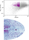 |
Fig. 2. Top: Mass-redshift distribution of the full eRASS1 galaxy cluster and group sample (gray) from Bulbul et al. (2024) and the clusters used in this work (purple). Bottom: Locations of the selected sample on the west Galactic hemisphere eRASS1 X-ray sky. |
2.2. Data reduction and surface brightness profile stacking
We analyzed the first four scans of the eROSITA All-Sky Survey (hereafter eRASS:4), which were collected from 12th December 2019 to 19th December 2021. The data were processed with the eSASS (Brunner et al. 2022) pipeline version 020, which is similar to the version 010 used for eRASS1 data release with improvements on boresight correction, detector noise suppression, and subpixel position computation (see Merloni et al. 2024, for the details). We only selected the events from telescope modules (TMs) 1,2,3,4,6 (hereafter TM8) to avoid the systematic uncertainties caused by the optical light leak in TMs 5 and 7 (Predehl et al. 2021). We used the tools in the eSASS software package, version eSASSusers_211214_0_4, to generate eRASS data products.
We adopted the full soft band 0.2–2.3 keV to maximize the signal-to-noise ratio. For each cluster, we created the count image using evtool and generated the corresponding vignetting corrected exposure map using expmap. The count map and exposure map are centered at the cluster X-ray centroid and are extended to an angular distance of 10 × r500c + 3.5°, where the 10 × r500c aperture is used for analysis, and the additional 3.5° annulus is for calculating the stray light from the sources outside the analysis region.
2.2.1. Source masks
We masked out different source types for each cluster field. These sources include
-
X-ray point sources in eRASS:4 catalog, where the source detection method and analysis are described in Merloni et al. (2024). We note that in a cluster field, especially in the central bright region, the source-detection configuration used for the master catalog yields spurious point source entries (Merloni et al. 2024). We removed these spurious sources by running an additional wavelet detection process in the r < r500 region. We first ran the software WVDECOMP4 with both detection and filtering thresholds (3, 3, 3, 4, 4) at scales (8, 16, 32, 64, 128)″. Then we ran the software SEXTRACTOR on the wavelet-filtered image to identify sources, with a detection threshold setting of 10. We cross-matched the wavelet-detected sources with those in the eRASS:4 master catalog. In the r < 0.8 × r500c region, we only masked out sources identified by both methods. We visually inspected the resulting mask maps and verified the robustness of spurious source cleaning using the parameters mentioned above.
-
Galaxy clusters and groups. We followed Zhang et al. (2024) to mask out 1) X-ray selected galaxy clusters and groups in the eRASS1 cluster catalog (Bulbul et al. 2024) with masking radii 1.5r500c; and 2) optically selected richness λ > 20 clusters5 with masking radii 1.5rλ (see Eq. (4) in Rykoff et al. 2014 for definition).
2.2.2. Stray light
The cluster emission in the regions we are interested in is below the sky background. Therefore, the stray light from eROSITA, the 3.5°-radius halo around any source produced by single-reflected photons, could affect the stacked profile and needs to be removed. We followed the recipe described in appendix A of Churazov et al. (2023) to correct for stray light contamination. In short, for each object, we first estimated the sky background level as the average count rate in the source-free region. Then we convolved the sky background-subtracted and vignetting-corrected count rate image with a kernel of the stray light profile (Eq. (A.2) in Churazov et al. 2023) to obtain a first-order approximation of the stray light count rate. The normalization of the stray light kernel was computed as the fraction of the 2D stray light profile volume with respect to the 2D volume of the total point spread function (PSF) (Eq. (A.1) + Eq. (A.2) in Churazov et al. 2023).
2.2.3. Profile stacking
The image products we created have pixel widths of 8″, resulting in a total number of 6.5 × 108 pixels for stacking. Meanwhile, this pixel size is smaller than the 30″ PSF half-energy width of the eRASS. To boost the calculation speed and save the memory space, we binned the original pixels to a Nside = 4096 hierarchical equal area isolatitude pixelization (HEALPix) scheme following the method described in Zhang et al. (2024).
For each object, we extracted a count profile and an exposure profile from the count and exposure maps, respectively. The radii of the profiles are scaled to r200m of the object, which was converted from r500c by assuming an Navarro-Frenk-White (NFW) profile with the halo concentration parameter c200c = 4. This value approximately represents the concentration of halos in the cluster mass range of the sample (e.g., Child et al. 2018; Diemer & Joyce 2019; Ishiyama et al. 2021; Okabe et al. 2025). The conversion factor has a redshift dependence, ranging from 2.48 at z = 0.034 to 2.24 at z = 0.2 within our sample.
We stacked the surface brightness profiles using a weight inversely proportional to the projected sky solid angle. The weight of each object  corrects for the potential bias from nearby objects and massive objects that are of a large angular size, where DA is the angular diameter distance as a function of redshift. The stacked surface brightness profile is
 (1)
(1)
where Ni(r) the ith count profile, ti(r)Ωi(r) the ith exposure profile in unit of s−1 deg−2. We used the HEALPix oriented bootstrap resampling method described in Zhang et al. (2024) to estimate the uncertainty of the stacked profile. We generated 500 bootstrapping samples of the HEALPix pixels from the full pixel list, and for each bootstrapping sample, we calculated a stacked profile using Eq. (1). Throughout this paper, we use the mean and covariance matrix of the 500 bootstrapping sample profiles to represent the stacked profile and its uncertainty.
3. Stacked eROSITA surface brightness profile and modeling
The stacked profile of the 680 galaxy clusters from 0.01 to 4 r200m is shown in Fig. 3. As expected, the background level is consistent with the values in the 0.2–2.3 keV reported by Zheng et al. (2024), which is ∼15 cts s−1 deg−2 in the Galactic anti-center region with the instrumental background included. The high S/N of the stacked profile allows us to probe the extremely weak signal at the background-dominant radii. The inset in Fig. 3 shows that there is still a significant positive signal above the local background level at r > r200m. Based on bootstrap sampling, the averaged surface brightness in the 1–2r200m range is higher than in the 2–4r200m range with a significance of 12σ. We conclude that this constitutes a significant detection of the signal up to 2 × r200m, which is approximately 4.5 Mpc given the median mass and redshift ranges of our sample. At ∼2 × r200m, there is a plausible bump. We investigated it by separating each cluster into four 90° sectors and stacking each of the sectors (see Appendix A). We find that this feature is contributed by fluctuations in the first sector and is not universal across all sectors. Meanwhile, in Appendix B, we performed a test of stacking signals with cluster positions randomly distributed on the sky. This experiment shows that the uncertainty from uncorrelated components is less than 0.3% of the background level. The test indicates that the detected signal does not arise from a background fluctuation in this background-dominated regime, but instead originates from X-ray emission in the circumcluster accretion region. In the following subsections, we model the stacked surface brightness profile in the full radial range out to 4r200m.
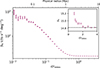 |
Fig. 3. Stacked eROSITA surface brightness profile in the 0.2–2.3 keV band after the stray light component was removed. The radial distance to the cluster center is scaled to the overdensity radius r200m. The corresponding physical radius given the sample median mass and redshift is labeled at the top of the figure. The top-right inset provides a zoomed-in view of the profile within a zoomed surface brightness range around the background level, with the dashed horizontal line indicating the average surface brightness between 3 and 4 r200m. The profile shows significant X-ray emission extended to approximately 2 × r200m. |
3.1. Model formalism
Numerical simulations suggest that both the dark matter and gas density profiles from halo center to a few r200m can be separated as inner and outer parts (e.g., Diemand & Kuhlen 2008; O’Neil et al. 2021; Diemer 2022; García et al. 2023). The inner profile is contributed by the matter orbiting within the halo, and the outer profile is contributed by infalling matter in the ambient accretion region, for example, nearby cosmic filaments and halos therein. The transition between the two regions is characterized by a sharp change in slope. This feature has been observed in SZ stacking (e.g. Anbajagane et al. 2022, 2024) and weak lensing shear stacking (e.g. Chang et al. 2018).
Numerous models for the inner and outer profiles have been proposed, some of which we later test in Section 4.1. To fit our observed data, we adopted a relatively simple prescription based on the halo model, which is commonly used to describe large-scale clustering (see Cooray & Sheth 2002, for a review). Specifically, for the one-halo term, we adopted a generalized NFW (gNFW) profile,
![Mathematical equation: $$ \begin{aligned} n_\mathrm{H} ^\mathrm{gNFW} (r) = n_\mathrm{H,0} \times \frac{1}{\left(r/r_\mathrm{s} \right)^{\gamma }\left[1 + \left(r/r_\mathrm{s} \right)^\alpha \right]^{(\beta -\gamma )/\alpha }}, \end{aligned} $$](/articles/aa/full_html/2026/05/aa57423-25/aa57423-25-eq3.gif) (2)
(2)
where α, β, γ, and rs are the four shape parameters. The gNFW model has been widely used to describe the pressure profile of cluster gas (e.g., Nagai et al. 2007; Arnaud et al. 2010; Bulbul et al. 2010). Because the X-ray-emitting gas in the off-filament directions terminates at the accretion shock, we also included this feature in the model. We assumed that the hot gas density in the downstream region after shock compression is the mean baryon density ⟨ρb⟩. The modified hydrogen density profile is then
 (3)
(3)
where ⟨nH⟩ is the mean hydrogen number density converted from ⟨ρb⟩. For our observed sample, ⟨nH⟩ = 3 × 10⁻⁷ cm−3 at the sample’s median redshift of 0.15. The gas density can be converted to an X-ray emission
 (4)
(4)
where we adopt ne = 1.2nH for the hot gas and Λcf(T, Z) is the temperature and metallicity-dependent cooling function. We projected the 3D emission onto a 2D plane. The projected surface X-ray photon rate is
 (5)
(5)
where l is the projection line-of-sight (LOS), lmax is the one side projection depth. With a flat sky approximation, the observed surface brightness
![Mathematical equation: $$ \begin{aligned} S_\mathrm{X} \left[\mathrm {cts\ s}^{-1}\ deg^{-2} \right] =&\Sigma _\mathrm{X} \left[\mathrm {cts\ s}^{-1}\ kpc^{-2} \right]\times A_\mathrm{eff} \left[\mathrm{cm} ^2\right] \\ &\times \frac{2.55\times 10^{-48}}{\left(1+z\right)^3}, \end{aligned} $$](/articles/aa/full_html/2026/05/aa57423-25/aa57423-25-eq7.gif) (6)
(6)
where Aeff is the averaged effective area of the observation band. We calculated ΛcfAeff in the 0.2–2.3 keV band 1) using the APEC model with ATOMDB v3.09 (Smith et al. 2001; Foster & Heuer 2020), 2) with an assumption of Z = 0.3 Z⊙ and Lodders et al. (2009) abundance table, 3) using the effective area curve of the five used eROSITA telescope modules, 4) applying a K-correction at z = 0.15, and 5) taking an averaged foreground the average HI column density of 3 × 1020 cm2 of the sample into account. The value of ΛcfAeff varies between 3 and 6 ph s−1 cm5 in the temperature range T > 3 × 10⁶ K. In this work, we adopted ΛcfAeff = 4.9 × 10⁻¹² ph s−1 cm5, which is the averaged value in the 3 × 10⁶ − 5 × 10⁷ K temperature range. In Appendix C, we present a more detailed investigation of the impact of different metallicity, foreground Galactic absorption, and radial temperature variation on the cooling function value. We conclude that the possible systematic uncertainty on the ΛcfAeff is ∼10%.
For the two-halo term, we started with theoretical calculations of the X-ray emission from nearby halos that are spatially correlated with the central halo. The distribution of neighbor halos around a halo can be described
 (7)
(7)
where Mc is the mass of the central halo, ξmmlin is the matter-matter correlation function in the linear regime, dn/dMdV is the halo mass function (HMF), b is the mass dependent halo bias parameter, which quantifies the excess clustering of halos over the clustering of dark matter. We adopted HMF from Tinker et al. (2008) and halo bias from Tinker et al. (2010). The profile of ξmmlin and the models of halo bias and HMF are numerically implemented in the package COLOSSUS6 (Diemer 2018). With a halo luminosity-mass scaling relation, we converted the halo distribution to the emission distribution,
 (8)
(8)
where ϵ2h ≡ dLX, 2h/dV, LX(M) is the luminosity-mass scaling relation, Mmin and Mmax are the integration limits. We used a survey selection function to describe the halo masking. Therefore, we rewrote Eq. (8) to
![Mathematical equation: $$ \begin{aligned} \epsilon _\mathrm{2h} (r,M_\mathrm{c} ,z)&= \xi _\mathrm{mm} ^\mathrm{lin} (r,z)b(M_\mathrm{c} ,z)\nonumber \\ \times \int _0^{M_\mathrm{max} }&\frac{\mathrm{d} n(M,z)}{\mathrm{d} M\mathrm{d} V}b(M,z)\left[1-P_\mathrm{det} (M,z)\right]L_\mathrm{X} (M,z) \mathrm{d} M, \end{aligned} $$](/articles/aa/full_html/2026/05/aa57423-25/aa57423-25-eq10.gif) (9)
(9)
where Pdet(M, z) is the eRASS1 X-ray selection function (Clerc et al. 2024), Mmax is the mass threshold of masking objects in observations, which is approximately 1014.3 M⊙ given our λ = 20 richness threshold for source masking and the richness-mass scaling relation from Ghirardini et al. (2024). For the LX − M scaling relation, we adopted the one from Bulbul et al. (2019) and applied a factor of 1.4 to convert 0.5–2 keV luminosity to 0.2–2.3 keV luminosity. Similar to the one-halo component, we applied Eqs. (5) and (6) to ϵ2h to obtain the projected two-halo term model surface brightness, where we used an integration limit lmax = 100 Mpc. We created the individual object two-halo model, and then stacked them using Eq. (1) to obtain a synthesis model SX, halo2h(r) for fitting. To account for the emission from unvirialized filament gas, an additional free normalization parameter A2h was also included in the fitting. The final projected two-halo model can be expressed as
 (10)
(10)
We used a constant profile to account for background components not associated with our stacking objects. The uncorrelated components include the instrumental background, Galactic foreground, and the cosmic X-ray background.
3.2. Surface brightness profile fitting
We modeled the stacked eRASS:4 profiles using the Bayesian inference package POCOMC (Karamanis et al. 2022a,b). The likelihood is defined as ℒ = −χ2/2, where χ2 = (Sxdata − Sxmodel)T𝒞−1(Sxdata − Sxmodel) is a generalized form that takes the profile covariance into account. We applied flat priors for all parameters. We adopted the median and the 16th to 84th percentiles of the posterior as the best-fit parameter and the uncertainty range.
We fit the model combination of the gNFW, two-halo, and a constant to the 0.2–2.3 keV stacked profile. The best-fit parameters are listed in Table 1. In the left panel of Fig. 4, we plot each best-fit component of the stacked profile as well as the fit residual. The fitting illustrates that the r200m is approximately the boundary between the one-halo dominant and two-halo dominant regions. To check the necessity of including the two-halo term in the fitting, we also fit the profile using gNFW + constant model combination. The best-fit components are plotted in Fig. D.1. Without the two-halo term, there are more residuals in the range of 1 − 2 × r200m. Based on the Bayesian model comparison framework, we calculated the Bayes factor of the two fits, which is exp(11.5). It suggests that the fitting by including the two-halo term is decisively favored according to the Jeffreys’ scale (Jeffreys 1961) or a similar scale later suggested by Kass & Raftery (1995). The normalization of the two-halo term is 0.22 ± 0.03 cts s−1 deg−2 at r200m, corresponding to ∼1 × 1035 erg s−1 kpc−2 at the sample median redshift, which is at the same order of the magnitude of that from the recent galaxy-X-ray cross-correlation study (Comparat et al. 2025).
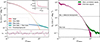 |
Fig. 4. Left: Best-fit results of the stacked 0.2–2.3 keV eROSITA surface brightness profile, where we adopted the gNFW model for the one-halo component. The width of each component denotes the 1σ scatter of the posterior samples. The inset shows a zoomed-in view around the background level. Right: Surface brightness profiles of the background-subtracted correlated signal (green) and the one-halo term signal. The systematic uncertainties of the uncorrelated background and the fitting uncertainties of the constant model and two-halo term normalization were propagated when calculating the profile uncertainty. |
Best-fit parameters of the gNFW gas density profile and the two-halo term normalization.
The fitting decomposes the total stacked signal into the uncorrelated signal, the two-halo term, and the one-halo term, allowing us to obtain the background-subtracted surface brightness profiles. In the right panel of Fig. 4, we plot the net correlated surface brightness profile and the net one-halo term surface brightness profile. The constant background and two-halo term normalization uncertainties from the fitting, as well as the systematic uncertainties of the uncorrelated background estimated by random position stacking in Appendix B, were propagated to compute the net profile uncertainties. The net surface brightness profile of the one-halo term decreases dramatically and enters the noise-dominant regime at r200m.
3.3. Density profile and comparison with the literature
We present the best-fit one-halo term gas number density profile in the left panel of Fig. 5. We note that the profile we show is the total gas number density ntot, where ntot = 2.3 × nH for typical halo gas. We present the profile uncertainty in two ways: the purple band is the 1σ scatter of the posterior sample from model inference; the red band is the range of the fitting results from four individual sectors. Due to the large pixel size we used for stacking, which is 0.86′, or 140 kpc physical scale at sample median redshift 0.15, we only show the density profile beyond 0.05 × r200m. Our best-fit density profile illustrates that the gas density at a large radius of r200m is still about 2.5 × 10⁻⁵ cm−3, corresponding to a baryon density contrast of 30. The cutoff of the profile at the cosmic averaged baryon density is introduced by the condition we applied in Eq. (3). We discuss it later in Sect. 5.2. In the right panel of Fig. 5, we present the best-fit density slope profile. The slope gradually steepens from −1 in central regions to −3 at r200m.
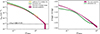 |
Fig. 5. Left: Best-fit gNFW gas number density profile 1σ posterior range (purple) and the range of individual fittings of the four wedges (red) inferred by the eROSITA observations. The result from L23 (yellow) up to 3 × r500c, and the result from Ghirardini et al. (2019) up to 2 × r500c (green). Right: The logarithmic radial density gradient from this work in purple and from Ghirardini et al. (2019) in green. |
Our best-fit density profile is overall consistent with the density profiles derived from the XMM-Newton and eROSITA observations of the Planck-selected samples out to two and three r500c (Ghirardini et al. 2019; L23), as shown in the left panel of Fig. 5. The normalization and slopes derived from the eROSITA observations of Planck-selected clusters in L23 are consistent with our fits in the radial range of 0.4 − 1 × r200m. Nonetheless, within the central region r < 0.4 × r200m, we find a slightly shallower slope and lower normalization. By contrast, the density profiles from the XMM-Newton observations in Ghirardini et al. (2019) show the highest normalization and the steepest slope compared to both our results and those of L23. A likely explanation for the offset observed in the central regions is the different mass ranges of the utilized samples. L23 stacked eROSITA observations of the Planck SZ sample (Planck Collaboration XXVII 2016) with a mass threshold of M500c > 2 × 10¹⁴ M⊙ and a mean mass of 4.1 × 10¹⁴ M⊙, while Ghirardini et al. (2019) used the X-COP sample (Eckert et al. 2017), which consists of 12 Planck-selected clusters with masses significantly higher than both our sample and that of L23. Thus, both comparison samples probe higher-mass clusters than those studied in this work, which could account for the observed offset.
4. Stacked profiles in IllustrisTNG simulation
In this section, we explore the galaxy cluster halos in the IllustrisTNG simulation to 1) validate our stacking and modeling processes; 2) compare the observations to the simulations to understand underlying physical processes in this unexplored region with previous observations; 3) study the 3D structure of the shock-heated gas from the galaxy cluster center to the accretion region. The IllustrisTNG is a suite of cosmological magnetohydrodynamical simulations (Naiman et al. 2018; Springel et al. 2018; Nelson et al. 2018; Marinacci et al. 2018; Pillepich et al. 2018) of galaxy formation in a fixed cosmology (Planck Collaboration XIII 2016). Halo and galaxy catalogs are based on the friend-of-friend (FoF) algorithm and subhalo/galaxy identification with Subfind (Springel et al. 2001).
For this work, we used the z = 0 snapshot of the highest-resolution version on the largest box, TNG300-1, to study the X-ray properties in cluster outskirts. Specifically, we selected 159 halos with M500c > 1014 M⊙ from the FoF catalog, whose mass range is comparable to the observation sample. We used the code HYDROTOOLS (Diemer et al. 2017b, 2018; Tacchella et al. 2019) to extract all gas cells out to 10 Mpc and calculate thermodynamic properties: (1) the total gas number density ntot = nH + ne + nHe, the sum of hydrogen, electron, and helium number density. The nH and nHe were converted from the mass density by assuming mass fractions of 0.76 and 0.24, respectively. The ne were calculated using the electron abundance of the cell. We ignored the contribution from metal elements in the total number density. (2) the gas temperature T, which was converted from the internal energy of the gas cell. (3) the electron entropy Ke = kBTene−2/3, where kB is the Boltzmann constant, Te = T by assuming the thermal equilibrium. (4) the gas pressure Pgas = ntotkBT.
In addition, we calculated the 0.2–2.3 keV X-ray emission properties under the assumption of collisional ionization equilibrium and using the ATOMDB v3.09 APEC code (Smith et al. 2001; Foster & Heuer 2020). For each gas cell,
![Mathematical equation: $$ \begin{aligned} L_\mathrm{X}&=V_\mathrm{cell} n_\mathrm{H} n_\mathrm{e} \Lambda _{Z=0}(T)\nonumber \\&+Z_\mathrm{cell} V_\mathrm{cell} n_\mathrm{H} n_\mathrm{e} \left[\Lambda _{Z=Z_\odot }(T) - \Lambda _{Z=0}(T)\right], \end{aligned} $$](/articles/aa/full_html/2026/05/aa57423-25/aa57423-25-eq12.gif) (11)
(11)
where Vcell is the cell volume, Zcell is the cell metallicity in solar unit, ΛZ = 0 and ΛZ = Z⊙ are the cooling function with zero metallicity and solar metallicity (Lodders et al. 2009), respectively.
4.1. Projected emission profile and fitting method validation
In this subsection, we validated the profile fitting framework using numerical simulation data. We aim to investigate whether the fitting results from the profile modeling framework we applied in Sect. 3 could match the true 3D density profiles up to the accretion shock.
In each 20 × 20 × 20 Mpc3 box centered at each halo, we projected the 0.2–2.3 keV X-ray emission on the XY, YZ, and XZ planes, respectively. Then we created nearby (sub)halo masks for each object and each projection angle, using M500c thresholds of 1013, 1013.5, and 1014 M⊙. We note that some of the bright X-ray halos in binary or multi-object systems are not identified as the main halo. We therefore excluded Subfind halos instead of FoF halos with a masking radius of 1.5r500c. Though the overdensity mass is not in the Subfind catalog, it can be converted from Msubfind. For most central halos, the ratio between M500c and Msubfind is about 2/3. For other subhalos, though we do not exactly know this ratio, we continued using this mask routine, which still successfully removes particles in the central regions of galaxies. For each projection direction and halo mask threshold, we stacked the radially averaged projected emission profile
 (12)
(12)
where r is the radius in a unit of r200m, wi is the weight, and here we adopted r500c−2 to reduce the bias from the large physical size objects. We calculated the median profile from the three projection angles as the final stacked profile.
The stacked 0.2–2.3 keV Σx profile with the three nearby-halo masking thresholds is plotted in the left panel of Fig. 6 as shaded regions. The three stacked profiles are identical in the r < 0.7 × r200m radial range and turn flat at r ≳ r200m. The outer parts of the profiles are contributed by gaseous (sub)halos with masses below the masking threshold from the far outskirts to cosmic filaments, together with the unvirialized gas in filaments. Different halo masking thresholds result in different Σx normalizations of the outer profile. Meanwhile, the outer parts of the three stacked profiles show several enhancements, where the one in the 1014 M⊙ masking threshold profile is the most significant. These enhancements are from bright X-ray halos below the masking threshold, and as the threshold decreases, their significance to the overall emission becomes negligible.
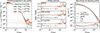 |
Fig. 6. Left: Stacked surface X-ray emission profiles of the TNG300-1 galaxy cluster halos. The teal, orange, and red colors denote the nearby-halos masking thresholds of 1013, 1013.5, and 1014 M⊙, respectively. The shaded regions represent the bootstrapped uncertainties, reflecting the sample scatter. The best-fit gNFW profiles, the two-halo terms, and the total profiles are plotted as dashed, dotted, and solid lines, respectively. The sharp peaks in the outer profile are contributed to by bright nearby halos that are below the masking threshold. Middle: The residuals of the fittings of the three different one-halo models. The χ2 values for each fit are labeled. Right: The best-fit total number density profiles and their comparison to the T > 106 K gas density profile in the off-filament directions in 3D (see Sect. 4.3). Different colors denote the different nearby halo masking thresholds of the stacked profiles, as in the left and middle panels. The dashed, dash-dotted, and dotted lines denote the results of the gNFW, V06, and L23 models, respectively. |
We followed Sect. 3 to fit the one-halo and two-halo models to the projected 2D simulated ΣX profiles. For the one-halo term, in addition to the gNFW model we used in Sect. 3, we included two more models for testing:
-
The Vikhlinin et al. (2006, hereafter V06) profile, which is
![Mathematical equation: $$ \begin{aligned} n_\mathrm{H} = n_\mathrm{H,0} \times \frac{\left( r/r_\mathrm{c} \right)^{-\alpha }}{\left[1 + (r/r_\mathrm{c} )^2\right]^{3\beta -\alpha /2}}\times \frac{1}{\left[1+(r/r_\mathrm{s} )^{\gamma }\right]^{\epsilon /\gamma }} , \end{aligned} $$](/articles/aa/full_html/2026/05/aa57423-25/aa57423-25-eq14.gif) (13)
(13)where nH, 0 is the hydrogen number density normalization, α, β, ϵ, γ, rc, and rs are the six parameters that control the profile shape.
-
The L23 profile, which is a modification of the V06 profile with an additional slope change at the large radii,
![Mathematical equation: $$ \begin{aligned} n_\mathrm{H} = n_\mathrm{H,0}&\times \frac{\left( r/r_\mathrm{c} \right)^{-\alpha }}{\left[1 + (r/r_\mathrm{c} )^2\right]^{3\beta -\alpha /2}}\times \frac{1}{\left[1+(r/r_\mathrm{s} )^{\gamma }\right]^{\epsilon /\gamma }}\nonumber \\&\times \frac{\left[1+(r/r_\mathrm{s2} )^\gamma \right]^{\epsilon /\gamma }}{\left[1+(r/r_\mathrm{s2} )^\xi \right]^{\lambda /\xi }} , \end{aligned} $$](/articles/aa/full_html/2026/05/aa57423-25/aa57423-25-eq15.gif) (14)
(14)
where λ, ξ, rs2 are three additional shape parameters.
We adopted a constant value Λcf = 8 × 10⁻²⁴ erg s−1 cm3 by assuming a constant temperature and abundance profile for the density to emissivity conversion. This is approximately the radiative cooling in the 0.2–2.3 keV band with T = 2 × 10⁷ K and Z = 0.3 Z⊙. As discussed in Sect. 3, a choice of a lower metallicity of 0.2 Z⊙ could result in a slightly lower Λcf. For the two-halo term formalism, there are several settings different from those we used in Sect. 3.1. First, we adopted the TNG300-1 LX − M scaling relation from Pop et al. (2022). Second, because the simulation data we extracted for each cluster are in 20 × 20 × 20 Mpc3 boxes, we used lmax = 10 Mpc as the one side projection depth when calculating the model ΣX using Eq. (5). Third, because we masked nearby halos in simulations only based on the mass, we did not further apply additional selection functions such as the one in Eq. (9).
We fit the three stacked profiles with the different mass exclusion thresholds, with the combined one-halo and two-halo terms. For each stacked profile, the three one-halo models were used separately for validation. We used the package IMINUIT (Dembinski et al. 2020) for minimizing the χ2 values. The left panel of Fig. 6 shows the results of the fits with the gNFW model as the one-halo component. The middle panel of Fig. 6 presents the residuals and best-fit χ2 values of the fits using the gNFW, V06, and L23 models on the three stacked profiles with different mass exclusion thresholds. The residuals show that all three one-halo models, together with the two-halo term, can well fit the projected emission profile from halo center to 4 × r200m. The three one-halo profile models return similar residuals and χ2 values. The large residual in fittings with a nearby halo masking threshold of 1014 M⊙ is due to several unmasked bright objects that are below the threshold. The right panel of Fig. 6 shows the best-fit one-halo density profiles of the gNFW, V06, and L23 models in dashed, dashed-dotted, and dotted lines, respectively, where different colors denote the different nearby halo masking thresholds. We overplot the scatter of the 3D density profiles in the off-filament directions as the gray shaded region (see later Sect. 4.3 for details). All the best-fit 3D density profiles using the three models are close to the true profiles. Among the three models we tested, the L23 model exhibits the most scatter, due to its additional flexibility in changing the slope at large radii, which allows it to overfit the features of the outer profile dominated by the two-halo term. Meanwhile, the fits using the gNFW model are in good agreement with those using the V06 model, despite having two fewer shape parameters. This comparison also highlights that the gNFW model can well describe the gas density profile out to large radii. Complex models with more shape parameters do not significantly improve the fitting residual.
This analysis shows that by adding a two-halo term to account for the nearby infalling (sub)halos and circumcluster gas in the cosmic filament directions, all three one-halo density models can well recover the true density profile in the off-filament directions out to the accretion shock in numerical simulations. In other words, the two-halo term accounts for the major gas-clumping effects, i.e., the presence of nearby (sub)halos and isotropic gas distribution due to cosmic filaments at large radii. The mild offset between the best-fit profile normalization and the median of the true 3D density profile can be explained by additional minor clumping effects, e.g., halo triaxiality, turbulence-induced density fluctuations, and the presence of inner shocks and cold fronts. Moreover, even if we assumed a constant cooling function and ignored variations in temperature and metallicity, the fits successfully recover the true number density profile, suggesting a minor impact from these two effects. We therefore conclude that our models, validated against the IllustrisTNG simulations, reliably recover the density profiles from the cluster cores out to the circumcluster region beyond r200m.
4.2. Comparison between simulations and observations
Different baryon-physics models, especially feedback models in hydrodynamic simulations, lead to large discrepancies in the gas distribution (e.g., Moser et al. 2022; Schaller et al. 2025). The observed eRASS profiles allow us to test the baryon-physics models of the TNG300-1 simulations. The normalization and slope of the inner profile characterize the spatial distribution of hot gas within the halo, reflecting its thermodynamic structure and underlying thermal and nonthermal effects. The outer profile reflects both the amounts of hot gas and gas-rich halos in the circumcluster or filament regions. In this section, we compare the observed profiles with the simulated profiles in the TNG300-1. Before the comparison, we applied the eRASS:1 cluster selection to the simulation sample. We adopted the mass and redshift dependent selection function Pdet(M, z) from Clerc et al. (2024). For each halo in the simulation sample, the detection probability as a function of mass is
 (15)
(15)
where P(z)∝dVcov/dz is the p.d.f. of the halo at different redshifts, which is scaled with the differential comoving volume. When calculating a selection-applied simulation profile, we used Pdet(M) as the averaging weight. We note again that the simulation data are from the z = 0 snapshot. Here we ignored the redshift evolution of halo properties and the HMF difference from 0.2 to 0.
We first compare the projected X-ray emission profile ΣX between observations and simulations in the left panel of Fig. 7. The eRASS observed ΣX profile (purple error bars) is the total SX profile with the best-fit uncorrelated component (see Sect. 3) subtracted and converted using Eq. (6). It includes both the one-halo and the two-halo components. In addition to the TNG300-1 simulations analyzed here, we include a comparison with two The Three Hundred (THE300) profiles reported by Li et al. (2025), from the Gizmo-Simba and Gadget-X runs (shown as dashed and dotted green lines, respectively). The same panel also displays the TNG300-1 simulation ΣX profile, with a nearby halo masking threshold of 1014 M⊙ indicated by the cyan-shaded region. In the inner region r ≲ r200m, the TNG300-1 ΣX profile is more centrally peaked compared to the stacked observations. In the radius range of 1 − 4r200m, the normalization of the TNG300-1 profile is a factor of 3 lower than the observations. This difference can be partly attributable to the limited projection depth of the TNG300-1 analysis (20 Mpc), which substantially reduces the projected two-halo signal.
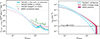 |
Fig. 7. Left: Comparison of the projected emission profiles from observations and simulations. The observed stacked eROSITA profile from this work is shown in purple error bars. The profiles extracted from the TNG300-1 simulation are shown as a cyan band. The TNG300-1 profile is more centrally peaked than the observed profile. For comparison, profiles of The Three Hundred Gizmo-Simba and Gadget-X simulations from Li et al. (2025) are shown as dashed and dotted green lines, respectively. Right: Best-fit gNFW gas number density profile 1σ posterior range (purple) and the range of individual fittings of the four wedges (red). We overplot the TNG300-1 gas number density profile in the off-filament directions (cyan-hatched region). |
Although the three simulation profiles are all calculated at z = 0 and with a nearby halo masking threshold of M500c = 1014 M⊙, the emissivity profiles of the two THE300 simulations have normalizations higher than those in the TNG300-1 in cluster outskirts to the circumcluster region, as shown in the left panel of Fig. 7. This could be partially attributed to the mass difference of the sample and the mass exclusion limit of the surrounding infalling halos. THE300 simulations only include massive halos with M200c > 1014.8 M⊙, whose halo bias is higher than the sample used in the TNG300-1. However, the one order-of-magnitude difference between the two profiles, Gizmo-Simba and Gadget-X, is due solely to the different simulation settings. As reported by Li et al. (2025), the Gadget-X run contains a higher fraction of dense gas at large radii. The comparison of the three profiles at large radii suggests that differences in the adoption of simulation codes, physical models, and model parameters could lead to a significant difference in the intensity of the circumcluster X-ray emission. The new stacked observations of the eROSITA clusters allow us to test physical models in these unexplored regions, from the cluster’s far outskirts to cosmic filaments.
As the next step, in the right panel of Fig. 7, we compare the one-halo term density profile from the eROSITA observations with the TNG300-1 T > 106 K hot gas density profiles in the off-filament direction (see the next subsection for details), where we use a blue hatched band to denote the 1σ scatter of the simulation profiles. As also shown in the ΣX profile comparison, the observed gas density profile is less centrally peaked than that predicted by the TNG300-1 simulation, suggesting that feedback processes in cluster-scale halos may be stronger and more efficient than those implemented in the IllustrisTNG model, displacing part of the gas toward the cluster outskirts. Similar discrepancies have been reported at lower halo masses in the galaxy group regime. The stacked kinematic SZ (kSZ) signal of luminous red galaxies measured by ACT appears more extended than the IllustrisTNG predictions (Hadzhiyska et al. 2025). Similarly, the eROSITA-selected galaxy groups tend to exhibit higher entropy from r2500c to r500c, corresponding to a lower central gas density compared to the MillenniumTNG simulations (Bahar et al. 2024), whose feedback model is similar to that of the TNG300-1 simulations used in this work. These results are also consistent with the systematically elevated normalization of the halo LX − M relation (Pop et al. 2022) and the higher gas mass fractions within r500c of the optically selected groups (Popesso et al. 2024). A detailed study of gas distribution with feedback models across a large mass range of eROSITA-selected galaxy clusters and groups will be presented in our upcoming studies (Ding et al. in prep., Clerc et al. in prep.).
4.3. Thermodynamic profiles in 3D
In this section, we investigate the thermodynamic properties of the gas from the halo center to the accretion regions in the TNG300-1 simulations. We extracted gas particles out to 5 r200m, and created masks for particles belonging to nearby halos and subhalos.
The spherically averaged gas density profiles from the cluster outskirts out to several r200m from hydrodynamic simulations consistently find that the profiles steepen from the cluster center to around r200m, before flattening again due to the influence of cosmic filaments (O’Neil et al. 2021; Angelinelli et al. 2022; Towler et al. 2024). However, in the following, we shall argue that at the radii with the presence of cosmic filaments, the gas properties toward the into-filament and off-filament (or into-void) environments could be significantly different and cannot be reflected by the spherically averaged profiles. Therefore, we aim to explore these quantities in both the filament and off-filament directions. Following Mansfield et al. (2017) and Aung et al. (2021), we adopted an Nside = 8 HEALPix scheme to group particles into 768 directions with respect to the halo center. For each LOS direction, we binned the volume-averaged radial profiles of T, Ke, Pgas, and ntot using 20 logarithmically spaced bins from 0.01 to 5 r200m. The temperature range of 105 − 105.5 K is usually the boundary between cool-to-warm and warm-hot gas (e.g., Cen & Ostriker 1999; van de Voort et al. 2011). Here we adopted a temperature threshold of 105 K to classify them into the in-filament and off-filament LOS directions. The into-filament/off-filament LOS profiles are those with the last radial bin temperature higher/lower than 105 K.
Figure 8 shows the 68% scatter of the 768 × 159 LOS profiles of T, Ke, Pgas, and ntot in the two different directions, where nearby M500c > 1013 M⊙ (sub)halos were excluded. For all the thermodynamic quantities of T, Ke, and Pgas, the into-filament and off-filament LOS profiles agree with each other within r200m and show a strong discrepancy beyond that radius. The into-filament temperature profiles keep T ∼ 106 K out to the maximum radius we extracted, while the off-filament-direction temperature profiles have more than two orders of magnitude drops at the radii of their accretion shocks, ∼2 − 3 r200m. Similarly, the discrepancy between the two directions and the feature of the accretion shock is also presented in the Ke and Pgas profiles. The ntot profile in the two directions deviates at r200m, but neither shows a jump at the shock radii. The absence of a strong jump in the total gas number density but a sharp drop in temperature is compatible with the Rankine-Hugoniot shock conditions, which impose limits of limℳ → ∞ρ2/ρ1 = 4 on the density jump and limℳ → ∞T2/T1 = 5/16 × ℳ2 on the temperature jump. For a high-ℳ accretion shock, the temperature can be enhanced by more than one order of magnitude, but the density enhancement is limited to 4. This change is smaller than the scatter of LOS ntot profiles among the cluster sample and could be easily smeared out due to the triaxiality of the shock surface. We also plot the off-filament direction gas number density profiles using gas cells with T > 106 K, which corresponds to the temperature range of X-ray-emitting gas. The gas number density profiles of the T > 106 K phase follow the total gas number density profile up to the termination at the accretion shock, which reflects that the hot gas in the off-filament direction is confined by the accretion shock. Outside the accretion shock, all gas is at temperatures below 106 K. This behavior matches the order-of-magnitude drop in the temperature profile.
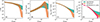 |
Fig. 8. One-σ scatter of the temperature (A), electron entropy (B), gas pressure (C), and gas density (D) line-of-sight profiles grouped into the filament (teal color) and off-filament directions (orange color) in the TNG300-1 simulations. All four profile types show a strong discrepancy in the two directions. In addition, we plot the T > 106 K gas density profile in the off-filament direction in magenta in panel D. The hot gas is confined by the accretion shock within 3 × r200m. |
5. Discussion
5.1. Clumping effects
hen measuring the halo gas density profile by deprojecting the 2D X-ray emission profile under the spherical symmetry assumption, gas clumping can overestimate the measured gas density, especially in the cluster outskirts. The clumping effects are quantified by a clumping factor
 (16)
(16)
In a broad sense, the clumping factor C(r) describes not only the presence of clump structures in and around the central halos e.g., gas rich subhalos and nearby cosmic filaments, but also other effects that violate the spherical symmetry assumption, e.g., large scale inhomogeneity, halo ellipticity, and gas density fluctuations due to turbulence, which are also termed as “residual clumpiness” (Roncarelli et al. 2013). Numerical simulations have quantified that C(r) is mild at intermediate radii due to the residual clumpiness and increases dramatically in the far outskirts due to the anisotropic gas distribution in the presence of connected cosmic filaments (e.g., Nagai & Lau 2011; Angelinelli et al. 2021). Pointing observations using XMM-Newton and Chandra also confirmed the mild gas clumping up to ∼r200c (e.g., Eckert et al. 2015; Zhu et al. 2023; Kovács et al. 2023).
In this work, we used the two-halo term to account for the emission from nearby halos and cosmic filaments, which is validated by the analysis of the TNG300-1 simulation in Sect. 4.1. With this method, we reduced the impact of the main clumpiness that leads to an overestimation of the gas density at r200m by a factor of a few (Nagai & Lau 2011; Angelinelli et al. 2021). However, residual clumping effects remain. Additionally, because we fit a single model to the stacked emission profile, the variance in the density profile of the stacking sample also introduces a similar “clumping” effect, i.e., the measured averaged density profile is weighted by individual source surface brightnesses scaled by ρgas(r)2. Although gas clumpiness varies across numerical simulation suites, our analysis of the TNG300-1 simulation sheds light on the possible residual clumpiness strength. The ratios between the best-fit density profiles and the sample median density profile (right panel of Fig. 6) indicate an overestimate of the gas density of 1.5 in the radial range of r500c < r < r200m. This possible clumping factor also agrees with the residual clumping factor value at ∼1.5 × r200c reported by Roncarelli et al. (2013).
5.2. Characteristic radii at the halo boundary
One important question in studying halos and structure formation is where a halo’s boundary lies. The infall, orbit, and turnaround of collisionless dark matter give rise to the splashback feature, which is now widely considered a novel definition of the halo boundary. However, the infall of collisional gas does not exhibit the splashback feature because it gets shocked before it can enter the halo. In this section, we discuss the possible characteristic radii of the gas content that can be constrained by our observations, and that could be used as halo boundaries, and the implications of these results.
The most prominent feature in both theoretical calculations and numerical simulations that can serve as the halo gas boundary is the accretion shock. In fact, the accretion shock in simulations is a gigantic structure enclosing the nodes, filaments, and sheets (e.g. Ryu et al. 2003; Schaal et al. 2016). For halos of galaxy clusters, in particular, our analysis of the LOS dependent thermodynamic profiles using TNG300-1 shows that the accretion shock is the boundary of hot gas in the off-filament direction.
In contrast to numerical simulations, it is extremely difficult to measure the accretion shock radius in observations. For example, Anbajagane et al. (2022) presented an SZ staking study but found only a marginal feature attributed to an average accretion shock at 4.6 × r200m. The projected surface brightness profile of the stacked eROSITA observations itself (see the left panel of Fig. 7) shows no clear surface brightness features corresponding to the accretion shock beyond r200m. Nevertheless, the profile fitting in this work provides an indirect clue to the accretion shock radius rshock, where the gas density reaches the post-shock density condition, rshock = r|ρ(r) = ρpost. The first assumption adopted is that ρpost = ⟨ρb⟩ in Eq. (3), which is supported by the TNG300-1 simulation. Our analysis of the simulation shows that the density profile in the off-filament direction (see the panel D of Fig. 8) reaches the accretion shock with a gas density 2 × 10⁻⁷ cm−3, slightly lower than the cosmic mean baryon density ⟨ρb⟩. In addition to our analysis of the TNG300-1 simulation, Vurm et al. (2023) analyzed the gas structure around the most massive halo in the C-EAGLE simulation, and their results also show that the post-shock gas density is slightly below ⟨ρb⟩. The second assumption is that the best-fit gNFW density profile within r200m can be extrapolated to larger radii, as supported by our TNG300-1 analysis. From our fitting results in Sect. 3, the gas density profile of the one-halo term reaches ⟨ρb⟩ at ∼3 × r200m, indicating a possible rshock based on our assumption. We clarify that this is a rough, indirect estimate based on the two assumptions mentioned above. A more generalized estimate can be expressed as
 (17)
(17)
Given the gas density contrast Δb ∼ 30 and the density slope dlog ρgas(r)/dlog r ∼ −3 at r200m, unless there is a sudden steepening of the gas density outside r200m or the post-shock density is much higher than ⟨ρb⟩, the rshock/r200m ratio is a factor of a few and not too close to 1.
Though the accretion shock is a prominent feature separating the void and the overdense cosmic web, mass accretion of galaxy clusters is mostly from the connected cosmic filaments. The high velocity infalling flows from cosmic filaments penetrate the outer atmosphere of the halo (e.g. Malavasi et al. 2023; Vurm et al. 2023; Rost et al. 2024). The model fitting of our observed profile directly reflects the radius of the halo-filament connection. In Fig. 4, the one-halo and two-halo terms intersect at ∼0.9 × r200m, shifting to ∼1.1 × r200m if we assume that 50% of the two-halo emission originates from nearby gas-rich halos. We could therefore still conclude that r200m approximately marks the halo–filament connection radius. Our analysis of the TNG300-1 simulation also suggests that the pressure and density LOS profiles in the filament direction deviate from those in the off-filament direction at roughly r200m. Our results of halo-filament connection radius are close to the “gas splashback radius” reported by O’Neil et al. (2021), Towler et al. (2024), who used the criteria of the steepest slope of radial gas density profile in the logarithmic space to characterize the radius. We argue that the presence of the steepest slope is necessary but not sufficient for claiming a splashback feature. The splashback is a feature of collisionless dark matter particles; the reported steepest slope is due to nearby filaments that flatten the spherically averaged radial density profile. Meanwhile, the halo-filament connection radius at r200m is approximately the inner shock location reported by Anbajagane et al. (2022, 2024) and the polarized stacked radio emission reported in Vernstrom et al. (2023), suggesting the discovered shock signal is due to the gas inflows from cosmic filaments.
5.3. Two-halo term normalization
When we fit the two-halo term, the model (Eq. (10)) includes a free normalization parameter A2h and a theoretical prediction of the profile. For the component of theoretical prediction, its profile shape is from ξmmlin, and the normalization depends on the halo bias, HMF, LX − M relation, and the selection function of masked sources. In principle, if the theoretical prediction of the two-halo term is accurate, the best-fit value of A2h indicates that, in addition to the X-ray emission from correlated nearby halos, the amount of X-ray emission from unvirialized gas in nearby cosmic filaments is required to match the observation. In our case, the predicted normalization is 3.7 × 1034 erg s−1 kpc−2 and the best-fit log A2h = 0.37 ± 0.06, which means that only ∼40% of the two-halo term emission is from the model prediction. We note that our theoretical prediction uses models of the Tinker et al. (2010) halo bias b, the Tinker et al. (2008) HMF, and the Bulbul et al. (2019)LX − M relation. To understand the impact of model adoption on the theoretical prediction of the two-halo normalization, we tested additional combinations of HMF models from Watson et al. (2013), Bocquet et al. (2016), Despali et al. (2016); halo bias models from Bhattacharya et al. (2011), Comparat et al. (2017), Pillepich et al. (2010); scaling relation model from Lovisari et al. (2020) and Chiu et al. (2022). The predicted two-halo emission ranges from 1.7 × 1034 to 7 × 1034 erg s−1 kpc−2. The large range of the predicted two-halo normalization indicates that, though the fraction of unvirialized gas emission is positive, it is difficult to have a precise constraint.
We note that the present two-halo model formalism focuses on the effects relevant to our analysis. In this context, we did not explicitly incorporate the scatter in the LX − M and Λ − M scaling relations. Consequently, the mass-dependent selection function and mass cut in Eq. (9) provide an approximate representation of the source masking scheme. Second, the two-halo term is modeled without including a contribution from unresolved active galactic nuclei (AGN). In addition, the X-ray properties of circumcluster halos may reflect aspects of their assembly history or ongoing ram-pressure stripping. Effects not captured by the current framework could influence theoretical predictions. Nevertheless, the robust detection of the two-halo signal at a background level of ≲2% highlights the importance of using next-generation X-ray missions, such as NewAthena (Cruise et al. 2025), to probe physical processes associated with cluster formation and ongoing mass accretion in these regions. This work provides a foundational investigation in the X-ray regime.
5.4. Gas fraction out to r200m
The reported gas mass fraction of halos within r500c is lower than the cosmic baryon fraction, and the depletion of the gas content is a function of halo mass (see the review of Eckert et al. 2021, and references therein). With the best-fit gas density profile in Sect. 3, we can measure the baryon density and therefore mass distribution beyond r500c by calculating a gas mass fraction profile.
The gas fraction is defined as
 (18)
(18)
where Mgas(r) and Mtot(r) are the gas mass and total mass within the radius r. We estimated Mtot(r) by assuming that the total mass of the halo follows an NFW profile. Due to the self-similar properties of the NFW model, the matter density profile in units of spherical overdensity radii only depends on the concentration parameter.
We used the hydrogen mass fraction of 0.71 to calculate fgas. This value is calculated with the assumptions of Lodders et al. (2009) abundance for Z = 0.3 Z⊙. Fig. 9 shows the fgas profile with respect to the cosmic baryon fraction with the adoption of c200c in [3,5] in the hatched magenta band. The fgas value continuously increases beyond r500c and reaches ≳100% of the cosmic baryon fraction at r200m. Since the stellar mass fraction additionally amounts to a few to ten percent of the cosmic baryon fraction (e.g. Gonzalez et al. 2013), the resulting total baryon fraction within r200m, including both the X-ray emitting gas and stellar components, is higher than the cosmic value, indicating possible gas clumping effects that overestimate the gas density. In an alternative calculation, we corrected for the gas density overestimation due to residual clumpiness. We applied the ratio between the best-fit and the sample median from the simulation analysis in Sect. 4.1 to the best-fit observed gas density profile. The resulting fgas profile is plotted as the filled magenta band in Fig. 9. The comparison shows that correcting for clumping significantly reduces the measured fgas in the outskirts. At r200m, the fgas profile with clumpiness correction is ∼80% of the cosmic mean baryon fraction. The profile also shows that the fgas, r500c with clumpiness correction is ∼65% of the cosmic mean baryon fraction, and is in line with the fgas − M relation from group size halos (Sun et al. 2009; Lovisari et al. 2015; Bahar et al. 2022; Bulbul et al. 2024; Siegel et al. 2025) to massive halos (Bulbul et al. 2012; Eckert et al. 2019; Bulbul et al. 2019; Liu et al. 2022; Bulbul et al. 2024) given the median mass M500c = 2.6 × 10¹⁴ M⊙ of our sample, though there is a 30% range of the measurements in literature (see fig. 7 in the review of Eckert et al. 2021).
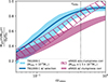 |
Fig. 9. Measured eROSITA gas fraction profiles with respect to the cosmic baryon fraction up to r200m and the comparison with simulations. The observed profile from observation with and without residual clumpiness correction is plotted in the hatched and filled magenta bands, respectively. The bandwidth represents the uncertainty from halo concentration c200c assumptions of from 3 to 5. The 1σ scatter of gas fraction profiles of M500c > 1014 M⊙ halos in the TNG300-1 simulations is plotted in a blue band, and the averaged gas fraction of halos with the selection function applied is plotted in the thick blue line. |
To compare the observed results with the TNG300-1 simulations. We calculated fgas for 159 galaxy clusters and show the 1σ scatter as the blue filled band in Fig. 9. Meanwhile, the averaged gas mass fraction with the selection function applied is plotted as the thick blue line. The fgas profiles of the TNG300-1 simulation reach an asymptotic value of 90% within r200m, and show a strong discrepancy with the observed fgas profile with clumpiness correction. The discrepancy is consistent with that observed in the density profile comparison in Sect. 4.2, reflecting that the IllustrisTNG model produces more concentrated gas density profiles. The observed 80% gas fraction with respect to the cosmic mean baryon density at r200m agrees more with simulations with stronger feedback models. For example, the Magneticum simulation shows similar values of fgas beyond r200c in bins of cluster masses (Angelinelli et al. 2022).
It is important to bear in mind that the residual clumpiness correction used in this section is based on our analysis of the TNG300-1 simulation. The strength of the correction reflects the large-scale gas inhomogeneity and the variance in density profiles among individual cluster halos in IllustrisTNG and may differ in other simulation suites. Moreover, we note an important caveat: beyond the systematic uncertainties in the total mass profile arising from the assumed concentration parameter (c200c = [3, 5]), the gas mass profile is subject to additional systematics not included in the total error budget. In particular, in this work, the conversion from gas density to X-ray emissivity relies on the assumption of a constant cooling function. If the true gas metallicity in the outskirts is lower than the assumed value, which is supported by numerical simulations, this would lead to an underestimation of both the gas mass profile and the fgas. Our investigations of the metallicity and temperature-dependent cooling function in Appendix C suggest a possible 10% underestimation if the metallicity is 0.2 Z⊙.
6. Conclusions
This study investigates the distribution of shock-heated gas from the outskirts of galaxy clusters into the large-scale accretion regions. We performed a stacking analysis of the two-year eROSITA All-Sky survey observations of 680 galaxy clusters selected in X-rays from the eRASS1 survey, spanning a mass range of M500c ≳ 1014 M⊙ and a redshift interval of 0.03 < z < 0.2 (Bulbul et al. 2024). At the 1 − 2 × r200m (∼2.3 − 4.5 Mpc) radii, we detected a statistically significant 12σ excess X-ray signal above the background. This represents the first detection of X-ray emission associated with galaxy clusters into the accretion region at large radii.
We modeled the stacked surface brightness profile as a superposition of one-halo, two-halo, and constant components, corresponding respectively to X-ray emission from the primary cluster halo, correlated structures such as infalling halos and filamentary gas, and the uncorrelated foreground/background. The best-fit results show that at r200m, the gas density is ∼2.5 × 10⁻⁵ cm−3, corresponding to a baryon density contrast of ∼30. Comparing the deprojected gas density profile derived from the one-halo term of the virialized gas to previous results in the literature, in the inner regions r < 0.1 × r200m, the profile shows slightly lower gas densities than those reported by Ghirardini et al. (2019) and L23, likely due to differences in the sample selection. In the intermediate radii, between 0.4 × r200m and 0.6 × r200m (approximately r500c to r200c), our results are consistent with those reported in the literature. The transition between the one-halo and two-halo regimes occurs around ∼r200m, suggesting that beyond this radius, the observed signal primarily is from unvirialized gas in connected filaments and nearby halos, under the detection limit of eROSITA.
We analyzed the TNG300-1 simulation to investigate the anisotropic distribution of the intracluster and circumcluster gas and to compare it with the observations. The thermodynamic profiles of the shock-heated gas exhibit clear directional dependence relative to the cosmic filaments. Along off-filament directions, the high-entropy, hot gas is sharply truncated and confined by the accretion shock at r > r200m. In contrast, profiles along filament directions remain elevated out to the maximum extraction radius, consistent with continuous gas inflow from the cosmic filament. Furthermore, we used the TNG300-1 data to validate our modeling framework for stacked eROSITA observations. Incorporating a two-halo term that accounts for shock-heated gas and X-ray halos in filaments results in a best-fit one-halo profile that accurately recovers the gas density profile in off-filament directions.
The observed gas density profile is more extended, while the profiles predicted by the TNG300-1 numerical simulations are more concentrated. This trend is also reflected in the gas fraction profile of the stacked cluster of galaxies. The gas fraction profile of the TNG300-1 cluster sample exhibits a steep rise beyond > 0.1r200m compared to the observations. If we apply a correction for residual clumping in the density profiles, the observed gas fractions at all radii are lower than in the TNG300-1 simulation. The differences in observed density and gas fraction profiles suggest that the feedback processes in M500c > 1014 M⊙ halos may be stronger than modeled in IllustrisTNG. This behavior is consistent with the recently observed trends at lower mass halos in galaxy group regimes in ACT kSZ measurements (Hadzhiyska et al. 2025; Siegel et al. 2025) and the stacked eROSITA observation of X-ray and optically selected galaxy groups (Bahar et al. 2024; Popesso et al. 2024).
Comparing observations with simulations, we identified two characteristic radii in the accretion region of the cluster outskirts that mark transitions in the thermodynamic state of the intracluster and intergalactic gas, potentially defining physical halo boundaries in this region. The first is the halo–filament intersection radius, located at approximately r200m, where the two-halo term for the unvirialized gas and infalling halos in the filaments begins to dominate the stacked X-ray surface brightness profile over the one-halo term of the virialized intracluster gas, corresponding to the scale at which the gas density and pressure profiles along cosmic filament directions exceed those in the off-filament directions in the TNG300-1 simulations. The second is the accretion shock radius, estimated to lie at ∼3 × r200m, inferred by extrapolating the one-halo gas density to the cosmic mean baryon density, consistent with the simulation predictions from the IllustrisTNG. However, the current depth of the eROSITA All-Sky Survey and the background levels limit our study to regions beyond r200m and to the direct detection of accretion-shock features.
This work presents the eRASS stacking analysis of the shock-heated gas in cluster far outskirts and surrounding circumcluster accretion regions. The results represent the average properties of the sample studied here. Detailed studies on individual systems require high sensitivity, low instrumental background, an understanding of the foreground/background large-scale structure, and deep exposure. The upcoming NewAthena mission (Nandra et al. 2013; Cruise et al. 2025) in the late 2030s will be particularly well-suited for such targeted studies of individual galaxy clusters, providing new insights into the cluster–filament connection, the anisotropic distribution of gas at cluster boundaries, and the emission contribution from unvirialized gas within filaments.
Acknowledgments
The authors thank the referee for their insightful comments, which helped improve the manuscript. The authors acknowledge Lars Hernquist and Volker Springel for helpful discussions. This work is based on data from eROSITA, the soft X-ray instrument aboard SRG, a joint Russian-German science mission supported by the Russian Space Agency (Roskosmos), in the interests of the Russian Academy of Sciences represented by its Space Research Institute (IKI), and the Deutsches Zentrum für Luft- und Raumfahrt (DLR). The SRG spacecraft was built by Lavochkin Association (NPOL) and its subcontractors, and is operated by NPOL with support from the Max Planck Institute for Extraterrestrial Physics (MPE). The development and construction of the eROSITA X-ray instrument was led by MPE, with contributions from the Dr. Karl Remeis Observatory Bamberg & ECAP (FAU Erlangen-Nuernberg), the University of Hamburg Observatory, the Leibniz Institute for Astrophysics Potsdam (AIP), and the Institute for Astronomy and Astrophysics of the University of Tübingen, with the support of DLR and the Max Planck Society. The Argelander Institute for Astronomy of the University of Bonn and the Ludwig-Maximilians-Universität München also participated in the science preparation for eROSITA. The eROSITA data shown here were processed using the eSASS/NRTA software system developed by the German eROSITA consortium. X. Zhang, E. Bulbul, E. Artis, and S. Zelmer acknowledge financial support from the European Research Council (ERC) Consolidator Grant under the European Union’s Horizon 2020 research and innovation program (grant agreement CoG DarkQuest No 101002585). A.L. acknowledges the support from the National Natural Science Foundation of China (Grant No. 12588202). A.L. is supported by the China Manned Space Program with grant no. CMS-CSST-2025-A04.
References
- Adhikari, S., Dalal, N., & Chamberlain, R. T. 2014, JCAP, 2014, 019 [Google Scholar]
- Anbajagane, D., Chang, C., Jain, B., et al. 2022, MNRAS, 514, 1645 [NASA ADS] [CrossRef] [Google Scholar]
- Anbajagane, D., Chang, C., Baxter, E. J., et al. 2024, MNRAS, 527, 9378 [Google Scholar]
- Angelinelli, M., Ettori, S., Vazza, F., & Jones, T. W. 2021, A&A, 653, A171 [NASA ADS] [CrossRef] [EDP Sciences] [Google Scholar]
- Angelinelli, M., Ettori, S., Dolag, K., Vazza, F., & Ragagnin, A. 2022, A&A, 663, L6 [NASA ADS] [CrossRef] [EDP Sciences] [Google Scholar]
- Arnaud, M., Pratt, G. W., Piffaretti, R., et al. 2010, A&A, 517, A92 [CrossRef] [EDP Sciences] [Google Scholar]
- Aung, H., Nagai, D., & Lau, E. T. 2021, MNRAS, 508, 2071 [NASA ADS] [CrossRef] [Google Scholar]
- Bahar, Y. E., Bulbul, E., Clerc, N., et al. 2022, A&A, 661, A7 [NASA ADS] [CrossRef] [EDP Sciences] [Google Scholar]
- Bahar, Y. E., Bulbul, E., Ghirardini, V., et al. 2024, A&A, 691, A188 [NASA ADS] [CrossRef] [EDP Sciences] [Google Scholar]
- Baxter, E. J., Adhikari, S., Vega-Ferrero, J., et al. 2021, MNRAS, 508, 1777 [NASA ADS] [CrossRef] [Google Scholar]
- Bertschinger, E. 1985, ApJS, 58, 39 [Google Scholar]
- Bhattacharya, S., Heitmann, K., White, M., et al. 2011, ApJ, 732, 122 [NASA ADS] [CrossRef] [Google Scholar]
- Bocquet, S., Saro, A., Dolag, K., & Mohr, J. J. 2016, MNRAS, 456, 2361 [Google Scholar]
- Brunner, H., Liu, T., Lamer, G., et al. 2022, A&A, 661, A1 [NASA ADS] [CrossRef] [EDP Sciences] [Google Scholar]
- Bulbul, G. E., Hasler, N., Bonamente, M., & Joy, M. 2010, ApJ, 720, 1038 [NASA ADS] [CrossRef] [Google Scholar]
- Bulbul, G. E., Smith, R. K., Foster, A., et al. 2012, ApJ, 747, 32 [NASA ADS] [CrossRef] [Google Scholar]
- Bulbul, E., Randall, S. W., Bayliss, M., et al. 2016, ApJ, 818, 131 [Google Scholar]
- Bulbul, E., Chiu, I. N., Mohr, J. J., et al. 2019, ApJ, 871, 50 [Google Scholar]
- Bulbul, E., Liu, A., Kluge, M., et al. 2024, A&A, 685, A106 [NASA ADS] [CrossRef] [EDP Sciences] [Google Scholar]
- Cen, R., & Ostriker, J. P. 1999, ApJ, 514, 1 [NASA ADS] [CrossRef] [Google Scholar]
- Chang, C., Baxter, E., Jain, B., et al. 2018, ApJ, 864, 83 [NASA ADS] [CrossRef] [Google Scholar]
- CHEX-MATE Collaboration (Arnaud, M., et al.) 2021, A&A, 650, A104 [NASA ADS] [CrossRef] [EDP Sciences] [Google Scholar]
- Child, H. L., Habib, S., Heitmann, K., et al. 2018, ApJ, 859, 55 [NASA ADS] [CrossRef] [Google Scholar]
- Chiu, I. N., Ghirardini, V., Liu, A., et al. 2022, A&A, 661, A11 [NASA ADS] [CrossRef] [EDP Sciences] [Google Scholar]
- Churazov, E., Khabibullin, I., Bykov, A. M., Lyskova, N., & Sunyaev, R. 2023, A&A, 670, A156 [NASA ADS] [CrossRef] [EDP Sciences] [Google Scholar]
- Clerc, N., Comparat, J., Seppi, R., et al. 2024, A&A, 687, A238 [NASA ADS] [CrossRef] [EDP Sciences] [Google Scholar]
- Comparat, J., Prada, F., Yepes, G., & Klypin, A. 2017, MNRAS, 469, 4157 [NASA ADS] [CrossRef] [Google Scholar]
- Comparat, J., Merloni, A., Ponti, G., et al. 2025, A&A, 697, A173 [NASA ADS] [CrossRef] [EDP Sciences] [Google Scholar]
- Cooray, A., & Sheth, R. 2002, Phys. Rep., 372, 1 [Google Scholar]
- Cruise, M., Guainazzi, M., Aird, J., et al. 2025, Nat. Astron., 9, 36 [Google Scholar]
- Dembinski, H., Ongmongkolkul, P., Christoph, D., et al. 2020, https://doi.org/10.5281/zenodo.3949207 [Google Scholar]
- Despali, G., Giocoli, C., Angulo, R. E., et al. 2016, MNRAS, 456, 2486 [NASA ADS] [CrossRef] [Google Scholar]
- Dey, A., Schlegel, D. J., Lang, D., et al. 2019, AJ, 157, 168 [Google Scholar]
- Diemand, J., & Kuhlen, M. 2008, ApJ, 680, L25 [NASA ADS] [CrossRef] [Google Scholar]
- Diemer, B. 2018, ApJS, 239, 35 [NASA ADS] [CrossRef] [Google Scholar]
- Diemer, B. 2022, MNRAS, 513, 573 [NASA ADS] [CrossRef] [Google Scholar]
- Diemer, B., & Joyce, M. 2019, ApJ, 871, 168 [NASA ADS] [CrossRef] [Google Scholar]
- Diemer, B., & Kravtsov, A. V. 2014, ApJ, 789, 1 [NASA ADS] [CrossRef] [Google Scholar]
- Diemer, B., Mansfield, P., Kravtsov, A. V., & More, S. 2017a, ApJ, 843, 140 [NASA ADS] [CrossRef] [Google Scholar]
- Diemer, B., Sparre, M., Abramson, L. E., & Torrey, P. 2017b, ApJ, 839, 26 [Google Scholar]
- Diemer, B., Stevens, A. R. H., Forbes, J. C., et al. 2018, ApJS, 238, 33 [NASA ADS] [CrossRef] [Google Scholar]
- Eckert, D., Molendi, S., Vazza, F., Ettori, S., & Paltani, S. 2013, A&A, 551, A22 [NASA ADS] [CrossRef] [EDP Sciences] [Google Scholar]
- Eckert, D., Roncarelli, M., Ettori, S., et al. 2015, MNRAS, 447, 2198 [Google Scholar]
- Eckert, D., Ettori, S., Pointecouteau, E., et al. 2017, Astron. Nachr., 338, 293 [Google Scholar]
- Eckert, D., Ghirardini, V., Ettori, S., et al. 2019, A&A, 621, A40 [NASA ADS] [CrossRef] [EDP Sciences] [Google Scholar]
- Eckert, D., Gaspari, M., Gastaldello, F., Le Brun, A. M. C., & O’Sullivan, E. 2021, Universe, 7, 142 [NASA ADS] [CrossRef] [Google Scholar]
- Fillmore, J. A., & Goldreich, P. 1984, ApJ, 281, 1 [Google Scholar]
- Foster, A. R., & Heuer, K. 2020, Atoms, 8, 49 [NASA ADS] [CrossRef] [Google Scholar]
- García, R., Salazar, E., Rozo, E., et al. 2023, MNRAS, 521, 2464 [CrossRef] [Google Scholar]
- Ghirardini, V., Eckert, D., Ettori, S., et al. 2019, A&A, 621, A41 [NASA ADS] [CrossRef] [EDP Sciences] [Google Scholar]
- Ghirardini, V., Bulbul, E., Artis, E., et al. 2024, A&A, 689, A298 [NASA ADS] [CrossRef] [EDP Sciences] [Google Scholar]
- Gonzalez, A. H., Sivanandam, S., Zabludoff, A. I., & Zaritsky, D. 2013, ApJ, 778, 14 [Google Scholar]
- Gouin, C., Gallo, S., & Aghanim, N. 2022, A&A, 664, A198 [NASA ADS] [CrossRef] [EDP Sciences] [Google Scholar]
- Grandis, S., Ghirardini, V., Bocquet, S., et al. 2024, A&A, 687, A178 [NASA ADS] [CrossRef] [EDP Sciences] [Google Scholar]
- Hadzhiyska, B., Ferraro, S., Ried Guachalla, B., et al. 2025, Phys. Rev. D, 112, 083509 [Google Scholar]
- Ishiyama, T., Prada, F., Klypin, A. A., et al. 2021, MNRAS, 506, 4210 [NASA ADS] [CrossRef] [Google Scholar]
- Jeffreys, H. 1961, Theory of Probability, International Series of Monographs on Physics (Clarendon Press) [Google Scholar]
- Karamanis, M., Beutler, F., Peacock, J. A., Nabergoj, D., & Seljak, U. 2022a, MNRAS, 516, 1644 [Google Scholar]
- Karamanis, M., Nabergoj, D., Beutler, F., Peacock, J., & Seljak, U. 2022b, J. Open Source Software, 7, 4634 [Google Scholar]
- Kass, R. E., & Raftery, A. E. 1995, J. Am. Stat. Assoc., 90, 773 [Google Scholar]
- Kleinebreil, F., Grandis, S., Schrabback, T., et al. 2025, A&A, 695, A216 [NASA ADS] [CrossRef] [EDP Sciences] [Google Scholar]
- Kluge, M., Comparat, J., Liu, A., et al. 2024, A&A, 688, A210 [NASA ADS] [CrossRef] [EDP Sciences] [Google Scholar]
- Kovács, O. E., Zhu, Z., Werner, N., Simionescu, A., & Bogdán, Á. 2023, A&A, 678, A91 [NASA ADS] [CrossRef] [EDP Sciences] [Google Scholar]
- Lau, E. T., Nagai, D., Avestruz, C., Nelson, K., & Vikhlinin, A. 2015, ApJ, 806, 68 [NASA ADS] [CrossRef] [Google Scholar]
- Li, R., Cui, W., Liu, A., et al. 2025, A&A, 701, A37 [NASA ADS] [CrossRef] [EDP Sciences] [Google Scholar]
- Liu, A., Bulbul, E., Ghirardini, V., et al. 2022, A&A, 661, A2 [NASA ADS] [CrossRef] [EDP Sciences] [Google Scholar]
- Lodders, K., Palme, H., & Gail, H. P. 2009, Landolt Börnstein, 4B, 712 [Google Scholar]
- Lovisari, L., Reiprich, T. H., & Schellenberger, G. 2015, A&A, 573, A118 [NASA ADS] [CrossRef] [EDP Sciences] [Google Scholar]
- Lovisari, L., Schellenberger, G., Sereno, M., et al. 2020, ApJ, 892, 102 [Google Scholar]
- Lyskova, N., Churazov, E., Khabibullin, I. I., et al. 2023, MNRAS, 525, 898 [NASA ADS] [CrossRef] [Google Scholar]
- Malavasi, N., Aghanim, N., Tanimura, H., Bonjean, V., & Douspis, M. 2020, A&A, 634, A30 [NASA ADS] [CrossRef] [EDP Sciences] [Google Scholar]
- Malavasi, N., Sorce, J. G., Dolag, K., & Aghanim, N. 2023, A&A, 675, A76 [NASA ADS] [CrossRef] [EDP Sciences] [Google Scholar]
- Mansfield, P., Kravtsov, A. V., & Diemer, B. 2017, ApJ, 841, 34 [NASA ADS] [CrossRef] [Google Scholar]
- Marinacci, F., Vogelsberger, M., Pakmor, R., et al. 2018, MNRAS, 480, 5113 [NASA ADS] [Google Scholar]
- McCall, H., Reiprich, T. H., Veronica, A., et al. 2024, A&A, 689, A113 [NASA ADS] [CrossRef] [EDP Sciences] [Google Scholar]
- Merloni, A., Lamer, G., Liu, T., et al. 2024, A&A, 682, A34 [NASA ADS] [CrossRef] [EDP Sciences] [Google Scholar]
- Mirakhor, M. S., & Walker, S. A. 2020, MNRAS, 497, 3204 [Google Scholar]
- Moser, E., Battaglia, N., Nagai, D., et al. 2022, ApJ, 933, 133 [NASA ADS] [CrossRef] [Google Scholar]
- Nagai, D., & Lau, E. T. 2011, ApJ, 731, L10 [NASA ADS] [CrossRef] [Google Scholar]
- Nagai, D., Kravtsov, A. V., & Vikhlinin, A. 2007, ApJ, 668, 1 [Google Scholar]
- Naiman, J. P., Pillepich, A., Springel, V., et al. 2018, MNRAS, 477, 1206 [Google Scholar]
- Nandra, K., Barret, D., Barcons, X., et al. 2013, arXiv e-prints [arXiv:1306.2307] [Google Scholar]
- Nelson, D., Pillepich, A., Springel, V., et al. 2018, MNRAS, 475, 624 [Google Scholar]
- Okabe, N., Reiprich, T. H., Grandis, S., et al. 2025, A&A, 700, A46 [NASA ADS] [CrossRef] [EDP Sciences] [Google Scholar]
- O’Neil, S., Barnes, D. J., Vogelsberger, M., & Diemer, B. 2021, MNRAS, 504, 4649 [CrossRef] [Google Scholar]
- Ostriker, J. P., & McKee, C. F. 1988, Rev. Mod. Phys., 60, 1 [Google Scholar]
- Pillepich, A., Porciani, C., & Hahn, O. 2010, MNRAS, 402, 191 [NASA ADS] [CrossRef] [Google Scholar]
- Pillepich, A., Nelson, D., Hernquist, L., et al. 2018, MNRAS, 475, 648 [Google Scholar]
- Planck Collaboration V. 2013, A&A, 550, A131 [NASA ADS] [CrossRef] [EDP Sciences] [Google Scholar]
- Planck Collaboration XIII. 2016, A&A, 594, A13 [NASA ADS] [CrossRef] [EDP Sciences] [Google Scholar]
- Planck Collaboration XXVII. 2016, A&A, 594, A27 [NASA ADS] [CrossRef] [EDP Sciences] [Google Scholar]
- Planck Collaboration VI. 2020, A&A, 641, A6 [NASA ADS] [CrossRef] [EDP Sciences] [Google Scholar]
- Pop, A. R., Hernquist, L., Nagai, D., et al. 2022, arXiv e-prints [arXiv:2205.11528] [Google Scholar]
- Popesso, P., Biviano, A., Marini, I., et al. 2026, A&A, 707, A362 [NASA ADS] [CrossRef] [EDP Sciences] [Google Scholar]
- Predehl, P., Andritschke, R., Arefiev, V., et al. 2021, A&A, 647, A1 [EDP Sciences] [Google Scholar]
- Reiprich, T. H., Basu, K., Ettori, S., et al. 2013, Space Sci. Rev., 177, 195 [Google Scholar]
- Roncarelli, M., Ettori, S., Borgani, S., et al. 2013, MNRAS, 432, 3030 [NASA ADS] [CrossRef] [Google Scholar]
- Rost, A., Kuchner, U., Welker, C., et al. 2021, MNRAS, 502, 714 [Google Scholar]
- Rost, A. M., Nuza, S. E., Stasyszyn, F., et al. 2024, MNRAS, 527, 1301 [Google Scholar]
- Rykoff, E. S., Rozo, E., Busha, M. T., et al. 2014, ApJ, 785, 104 [Google Scholar]
- Ryu, D., Kang, H., Hallman, E., & Jones, T. W. 2003, ApJ, 593, 599 [NASA ADS] [CrossRef] [Google Scholar]
- Schaal, K., Springel, V., Pakmor, R., et al. 2016, MNRAS, 461, 4441 [NASA ADS] [CrossRef] [Google Scholar]
- Schaller, M., Schaye, J., Kugel, R., Broxterman, J. C., & van Daalen, M. P. 2025, MNRAS, 539, 1337 [Google Scholar]
- Shi, X. 2016, MNRAS, 461, 1804 [NASA ADS] [CrossRef] [Google Scholar]
- Siegel, J., Amon, A., McCarthy, I. G., et al. 2025, arXiv e-prints [arXiv:2509.10455] [Google Scholar]
- Simionescu, A., Allen, S. W., Mantz, A., et al. 2011, Science, 331, 1576 [Google Scholar]
- Smith, R. K., Brickhouse, N. S., Liedahl, D. A., & Raymond, J. C. 2001, ApJ, 556, L91 [Google Scholar]
- Springel, V., White, S. D. M., Tormen, G., & Kauffmann, G. 2001, MNRAS, 328, 726 [Google Scholar]
- Springel, V., Pakmor, R., Pillepich, A., et al. 2018, MNRAS, 475, 676 [Google Scholar]
- Sun, M., Voit, G. M., Donahue, M., et al. 2009, ApJ, 693, 1142 [NASA ADS] [CrossRef] [Google Scholar]
- Tacchella, S., Diemer, B., Hernquist, L., et al. 2019, MNRAS, 487, 5416 [Google Scholar]
- Tinker, J., Kravtsov, A. V., Klypin, A., et al. 2008, ApJ, 688, 709 [Google Scholar]
- Tinker, J. L., Robertson, B. E., Kravtsov, A. V., et al. 2010, ApJ, 724, 878 [NASA ADS] [CrossRef] [Google Scholar]
- Towler, I., Kay, S. T., Schaye, J., et al. 2024, MNRAS, 529, 2017 [NASA ADS] [CrossRef] [Google Scholar]
- van de Voort, F., Schaye, J., Booth, C. M., Haas, M. R., & Dalla Vecchia, C. 2011, MNRAS, 414, 2458 [NASA ADS] [CrossRef] [Google Scholar]
- Vernstrom, T., West, J., Vazza, F., et al. 2023, Sci. Adv., 9, eade7233 [NASA ADS] [CrossRef] [Google Scholar]
- Vikhlinin, A., Kravtsov, A., Forman, W., et al. 2006, ApJ, 640, 691 [Google Scholar]
- Vurm, I., Nevalainen, J., Hong, S. E., et al. 2023, A&A, 673, A62 [NASA ADS] [CrossRef] [EDP Sciences] [Google Scholar]
- Walker, S. A., Fabian, A. C., Sanders, J. S., Simionescu, A., & Tawara, Y. 2013, MNRAS, 432, 554 [Google Scholar]
- Walker, S., Simionescu, A., Nagai, D., et al. 2019, Space Sci. Rev., 215, 7 [Google Scholar]
- Watson, W. A., Iliev, I. T., D’Aloisio, A., et al. 2013, MNRAS, 433, 1230 [Google Scholar]
- Willingale, R., Starling, R. L. C., Beardmore, A. P., Tanvir, N. R., & O’Brien, P. T. 2013, MNRAS, 431, 394 [Google Scholar]
- Zhang, X., Bulbul, E., Malavasi, N., et al. 2024, A&A, 691, A234 [NASA ADS] [CrossRef] [EDP Sciences] [Google Scholar]
- Zheng, X., Ponti, G., Freyberg, M., et al. 2024, A&A, 681, A77 [NASA ADS] [CrossRef] [EDP Sciences] [Google Scholar]
- Zhu, Z., Kovács, O. E., Simionescu, A., & Werner, N. 2023, A&A, 678, A122 [NASA ADS] [CrossRef] [EDP Sciences] [Google Scholar]
- Zhuravleva, I., Churazov, E., Kravtsov, A., et al. 2013, MNRAS, 428, 3274 [NASA ADS] [CrossRef] [Google Scholar]
Throughout this paper, we use spherical overdensity to define halos’ mass and radius. For example, r500c is the radius where the enclosed density is 500 times the critical density ρc; and M200m is the total mass enclosed by r200m, where the enclosed density is 200 times the mean matter density ρm.
We follow the convention and use the term “accretion shock” to refer to the “external shock” in Ryu et al. (2003). In fact, the accretion shock is around all overdense environments, including cosmic filaments and sheets. In this work, we focus on the accretion shock around galaxy clusters.
The terms of the intracluster medium (ICM) and warm-hot intergalactic medium (WHIM) are usually used for the hot gas in galaxy clusters and cosmic filaments, respectively. Both gases are heated by cosmic accretion shocks as they accrete onto the cosmic web. At the radii where halos are connected with cosmic filaments, there is no clear boundary to distinguish the ICM and WHIM. Therefore, in this work, we use the term “shock-heated gas” to refer to the hot gas in both halos and cosmic filaments.
It is a proprietary catalog of redMaPPer (Rykoff et al. 2014) run on the DESI Legacy Imaging Surveys (Dey et al. 2019) DR10 data. See Kluge et al. (2024) for the description.
Total effective hydrogen column density by taking molecular into account (Willingale et al. 2013).
Appendix A: Profiles in four individual sectors
In the inset of Fig. 3, there is a plausible surface brightness jump at ∼2r200m. In this section, we explore the origin of this feature.
Following L23, we divided each cluster into four 90° sectors and stacked profiles of each. The comparison between the four sector profiles and the full profile is shown in Fig. A.1. The profile in sector 1 is the most scattered profile among the four. It shows features of a spike in the bin between 1.6 and 1.9 r200m and a dip in the bin between 2.2 and 2.6 r200m. The two features result in a plausible jump in the full profile. Because the jump is not a universal feature across all four sectors, we do not overinterpret it further.
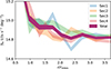 |
Fig. A.1. Comparison between the full stacked profile and those in four independent sectors. |
Appendix B: Noise level from the uncorrelated components
The stacking of randomly distributed objects in the sky filters out signals from uncorrelated components, such as the instrumental background, fluctuations in Galactic halo emission, and foreground absorption. To validate it and quantify the contribution of the uncorrelated components in the error budget, we performed stacking analysis on a sky map free of sources.
We first created an eRASS:4 HEALPix map in the 0.2-2.3 keV band with all sources removed (see Sect. 2.2.1 for the source catalogs). An example of the source masked sky rate map is shown in the left panel of Fig. B.1. Then, we randomly distributed the positions of the 680 galaxy clusters on the half-sky map. With the randomized cluster positions, we obtained a stacked surface brightness profile with the weights provided in Eq. 1. We repeated the randomization process 500 times to obtain a set of control sample profiles.
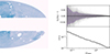 |
Fig. B.1. Left: Source removed eRASS:4 sky map for studying the uncorrelated background noise. Top right: Five-hundred control sample relative surface brightness profiles stacked with cluster positions randomly distributed on the sky. The shade region denotes the scatter of the 500 control sample profiles. Bottom right: The scatter of the 500 control sample profile as a function of the radius. As the radius increases, the scatter decreases. Beyond r200m, the scatter is smaller than 0.3% |
We aimed to study relative surface brightness fluctuations relative to the profile average. Therefore, for each profile, we divided individual bin values by the profile mean. On the right panel of Fig. B.1, we plot the relative profiles of the 500 control samples, where the 68% scatter is shown as the shaded region. On the bottom-right panel, we plot the relative scatter as a function of the radius. It shows that the 680 objects and the depth of the eRASS:4 sky result in a noise level below 0.3% from uncorrelated components. This 0.3% fluctuation can be treated as the systematic uncertainties of the stacked emission beyond r200m.
Appendix C: Impact of using a constant cooling function
In this section, we investigate the impact and possible systematic uncertainties of adopting a constant ΛcfAeff for fitting the stacked surface brightness profile. In reality, each object has its own temperature and metallicity profiles as well as a sky position-dependent foreground nH column density that attenuates the observed count rate.
For each cluster, we predicted the temperature profile by adopting eqs. 10 and 11 and the best-fit parameters therein from Ghirardini et al. (2019). The temperature-mass scaling relation is based on the self-similar theory T ∝ M2/3, and the profile shape is originally from Vikhlinin et al. (2006). Then we calculated the radial ΛcfAeff by plugging in the temperature profile, redshift, foreground nH, tot value7, and gas metallicity. We calculated profiles with both the 0.2 and 0.3 Z⊙ metallicity assumptions. The comparison between the constant value 4.9 × 10⁻¹² ph s−1 cm5 used in this work and the sample mean/median is shown in Fig. C.1.
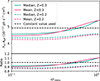 |
Fig. C.1. Top: Sample averaged (teal) and median (red) radial cooling functions that take individual cluster temperature profiles and foreground absorption strength into account. Solid and dashed lines denote metallicity assumptions of 0.3 and 0.2 Z⊙, respectively. The black-dashed line represents the constant cooling function used for model fitting in this work. Bottom: Ratios between radial cooling functions and the constant value used for model fitting. |
With the Z = 0.3 Z⊙ metallicity assumption, the sample average and median ΛcfAeff profiles are 10% lower than the constant value we used in the radial range r ≲ 0.5 × r200m and are 10% higher at large radii. The mild increase of the ΛcfAeff with radius is due to the decrease of the gas temperature in the outskirts. With the Z = 0.2 Z⊙ metallicity assumption, the ΛcfAeff is ∼10%−15% lower than the value used in this work at all radii. The lower radial dependence is due to the lower abundance of line emissions from the Fe-L complex, which reaches its highest emissivity at kT ∼ 1 keV.
Appendix D: Fitting without two-halo term
Fig. D.1 shows the best-fit components and residuals without the two-halo term. There are significant residuals at r > r200m in both the inset and the residual plot.
All Tables
Best-fit parameters of the gNFW gas density profile and the two-halo term normalization.
All Figures
|
Fig. 1. Spatial distribution of the X-ray emission from the hot gas around a massive dark matter halo. The dashed circle indicates the size of r200m. At large radii, the halo is connected to and accreting smaller nearby halos from cosmic filaments. This map is produced using gas particles from a 20 × 20 × 20 Mpc3 box around the id=32 halo in the z = 0 snapshot of the TNG300-1 simulation (see Sect. 4 for the details of map creation). The central halo is in a mass M500c = 2.8 × 10¹⁴ M⊙ and an r200m of 2.5 Mpc. Short arrows mark the accretion shock, i.e., the boundary between shock-heated gas and the cool intergalactic medium. |
| In the text | |
|
Fig. 2. Top: Mass-redshift distribution of the full eRASS1 galaxy cluster and group sample (gray) from Bulbul et al. (2024) and the clusters used in this work (purple). Bottom: Locations of the selected sample on the west Galactic hemisphere eRASS1 X-ray sky. |
| In the text | |
|
Fig. 3. Stacked eROSITA surface brightness profile in the 0.2–2.3 keV band after the stray light component was removed. The radial distance to the cluster center is scaled to the overdensity radius r200m. The corresponding physical radius given the sample median mass and redshift is labeled at the top of the figure. The top-right inset provides a zoomed-in view of the profile within a zoomed surface brightness range around the background level, with the dashed horizontal line indicating the average surface brightness between 3 and 4 r200m. The profile shows significant X-ray emission extended to approximately 2 × r200m. |
| In the text | |
|
Fig. 4. Left: Best-fit results of the stacked 0.2–2.3 keV eROSITA surface brightness profile, where we adopted the gNFW model for the one-halo component. The width of each component denotes the 1σ scatter of the posterior samples. The inset shows a zoomed-in view around the background level. Right: Surface brightness profiles of the background-subtracted correlated signal (green) and the one-halo term signal. The systematic uncertainties of the uncorrelated background and the fitting uncertainties of the constant model and two-halo term normalization were propagated when calculating the profile uncertainty. |
| In the text | |
|
Fig. 5. Left: Best-fit gNFW gas number density profile 1σ posterior range (purple) and the range of individual fittings of the four wedges (red) inferred by the eROSITA observations. The result from L23 (yellow) up to 3 × r500c, and the result from Ghirardini et al. (2019) up to 2 × r500c (green). Right: The logarithmic radial density gradient from this work in purple and from Ghirardini et al. (2019) in green. |
| In the text | |
|
Fig. 6. Left: Stacked surface X-ray emission profiles of the TNG300-1 galaxy cluster halos. The teal, orange, and red colors denote the nearby-halos masking thresholds of 1013, 1013.5, and 1014 M⊙, respectively. The shaded regions represent the bootstrapped uncertainties, reflecting the sample scatter. The best-fit gNFW profiles, the two-halo terms, and the total profiles are plotted as dashed, dotted, and solid lines, respectively. The sharp peaks in the outer profile are contributed to by bright nearby halos that are below the masking threshold. Middle: The residuals of the fittings of the three different one-halo models. The χ2 values for each fit are labeled. Right: The best-fit total number density profiles and their comparison to the T > 106 K gas density profile in the off-filament directions in 3D (see Sect. 4.3). Different colors denote the different nearby halo masking thresholds of the stacked profiles, as in the left and middle panels. The dashed, dash-dotted, and dotted lines denote the results of the gNFW, V06, and L23 models, respectively. |
| In the text | |
|
Fig. 7. Left: Comparison of the projected emission profiles from observations and simulations. The observed stacked eROSITA profile from this work is shown in purple error bars. The profiles extracted from the TNG300-1 simulation are shown as a cyan band. The TNG300-1 profile is more centrally peaked than the observed profile. For comparison, profiles of The Three Hundred Gizmo-Simba and Gadget-X simulations from Li et al. (2025) are shown as dashed and dotted green lines, respectively. Right: Best-fit gNFW gas number density profile 1σ posterior range (purple) and the range of individual fittings of the four wedges (red). We overplot the TNG300-1 gas number density profile in the off-filament directions (cyan-hatched region). |
| In the text | |
|
Fig. 8. One-σ scatter of the temperature (A), electron entropy (B), gas pressure (C), and gas density (D) line-of-sight profiles grouped into the filament (teal color) and off-filament directions (orange color) in the TNG300-1 simulations. All four profile types show a strong discrepancy in the two directions. In addition, we plot the T > 106 K gas density profile in the off-filament direction in magenta in panel D. The hot gas is confined by the accretion shock within 3 × r200m. |
| In the text | |
|
Fig. 9. Measured eROSITA gas fraction profiles with respect to the cosmic baryon fraction up to r200m and the comparison with simulations. The observed profile from observation with and without residual clumpiness correction is plotted in the hatched and filled magenta bands, respectively. The bandwidth represents the uncertainty from halo concentration c200c assumptions of from 3 to 5. The 1σ scatter of gas fraction profiles of M500c > 1014 M⊙ halos in the TNG300-1 simulations is plotted in a blue band, and the averaged gas fraction of halos with the selection function applied is plotted in the thick blue line. |
| In the text | |
|
Fig. A.1. Comparison between the full stacked profile and those in four independent sectors. |
| In the text | |
|
Fig. B.1. Left: Source removed eRASS:4 sky map for studying the uncorrelated background noise. Top right: Five-hundred control sample relative surface brightness profiles stacked with cluster positions randomly distributed on the sky. The shade region denotes the scatter of the 500 control sample profiles. Bottom right: The scatter of the 500 control sample profile as a function of the radius. As the radius increases, the scatter decreases. Beyond r200m, the scatter is smaller than 0.3% |
| In the text | |
|
Fig. C.1. Top: Sample averaged (teal) and median (red) radial cooling functions that take individual cluster temperature profiles and foreground absorption strength into account. Solid and dashed lines denote metallicity assumptions of 0.3 and 0.2 Z⊙, respectively. The black-dashed line represents the constant cooling function used for model fitting in this work. Bottom: Ratios between radial cooling functions and the constant value used for model fitting. |
| In the text | |
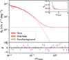 |
Fig. D.1. Same as Fig. 4 but without the two-halo term. Significant residuals at r > r200m exist. |
| In the text | |
Current usage metrics show cumulative count of Article Views (full-text article views including HTML views, PDF and ePub downloads, according to the available data) and Abstracts Views on Vision4Press platform.
Data correspond to usage on the plateform after 2015. The current usage metrics is available 48-96 hours after online publication and is updated daily on week days.
Initial download of the metrics may take a while.