| Issue |
A&A
Volume 700, August 2025
|
|
|---|---|---|
| Article Number | A11 | |
| Number of page(s) | 31 | |
| Section | Planets, planetary systems, and small bodies | |
| DOI | https://doi.org/10.1051/0004-6361/202553728 | |
| Published online | 29 July 2025 | |
Diving into the planetary system of Proxima with NIRPS
Breaking the metre per second barrier in the infrared★
1
Instituto de Astrofísica de Canarias (IAC),
Calle Vía Láctea s/n,
38205
La Laguna,
Tenerife,
Spain
2
Departamento de Astrofísica, Universidad de La Laguna (ULL),
38206
La Laguna,
Tenerife,
Spain
3
Institut Trottier de recherche sur les exoplanètes, Département de Physique, Université de Montréal,
Montréal,
Québec,
Canada
4
Observatoire du Mont-Mégantic,
Québec,
Canada
5
Observatoire de Genève, Département d’Astronomie, Université de Genève,
Chemin Pegasi 51,
1290
Versoix,
Switzerland
6
Univ. Grenoble Alpes, CNRS, IPAG,
38000
Grenoble,
France
7
Departamento de Física Teórica e Experimental, Universidade Federal do Rio Grande do Norte,
Campus Universitário,
Natal,
RN
59072-970,
Brazil
8
Instituto de Astrofísica e Ciências do Espaço, Universidade do Porto, CAUP, Rua das Estrelas,
4150-762
Porto,
Portugal
9
Departamento de Física e Astronomia, Faculdade de Ciências, Universidade do Porto, Rua do Campo Alegre,
4169-007
Porto,
Portugal
10
Department of Physics, University of Toronto,
Toronto,
ON
M5S 3H4,
Canada
11
Department of Physics & Astronomy, McMaster University,
1280 Main St W,
Hamilton,
ON
L8S 4L8,
Canada
12
Department of Physics, McGill University,
3600 rue University,
Montréal,
QC
H3A 2T8,
Canada
13
Department of Earth & Planetary Sciences, McGill University,
3450 rue University,
Montréal,
QC
H3A 0E8,
Canada
14
Departamento de Física, Universidade Federal do Ceará,
Caixa Postal 6030, Campus do Pici,
Fortaleza,
Brazil
15
Centro de Astrobiología (CAB),
CSIC-INTA, ESAC campus, Camino Bajo del Castillo s/n, 28692,
Villanueva de la Cañada (Madrid),
Spain
16
Centre Vie dans l’Univers, Faculté des sciences de l’Université de Genève,
Quai Ernest-Ansermet 30,
1205
Geneva,
Switzerland
17
European Southern Observatory (ESO),
Karl-Schwarzschild-Str. 2,
85748
Garching bei München,
Germany
18
Space Research and Planetary Sciences, Physics Institute, University of Bern,
Gesellschaftsstrasse 6,
3012
Bern,
Switzerland
19
Consejo Superior de Investigaciones Científicas (CSIC),
28006
Madrid,
Spain
20
Bishop’s Univeristy, Dept of Physics and Astronomy,
Johnson-104E, 2600 College Street,
Sherbrooke,
QC
J1M 1Z7,
Canada
21
Department of Physics and Space Science, Royal Military College of Canada,
PO Box 17000, Station Forces,
Kingston,
ON,
Canada
22
Instituto de Astrofísica e Ciências do Espaço, Faculdade de Ciên-cias da Universidade de Lisboa,
Campo Grande,
1749-016
Lisboa,
Portugal
23
Departamento de Física da Faculdade de Ciências da Universidade de Lisboa,
Edifício C8,
1749-016
Lisboa,
Portugal
24
Centre of Optics, Photonics and Lasers, Université Laval,
Québec,
Canada
25
Herzberg Astronomy and Astrophysics Research Centre, National Research Council of Canada,
Canada
26
Aix Marseille Univ, CNRS, CNES, LAM,
Marseille,
France
27
Center for Space and Habitability, University of Bern,
Gesellschaftsstrasse 6,
3012
Bern,
Switzerland
28
European Southern Observatory (ESO),
Av. Alonso de Cordova 3107,
Casilla
19001,
Santiago de Chile,
Chile
29
Planétarium de Montréal,
Espace pour la Vie, 4801 av. Pierre-de Coubertin,
Montréal,
Québec,
Canada
30
Lund Observatory, Division of Astrophysics, Department of Physics, Lund University,
Box 118,
221 00
Lund,
Sweden
31
York University,
4700 Keele St,
North York,
ON
M3J 1P3,
Canada
32
University of British Columbia,
2329 West Mall,
Vancouver,
BC
V6T 1Z4,
Canada
33
Western University, Department of Physics & Astronomy and Institute for Earth and Space Exploration,
1151 Richmond Street,
London,
ON
N6A 3K7,
Canada
34
Light Bridges S.L., Observatorio del Teide, Carretera del Observatorio,
s/n Guimar,
38500
Tenerife,
Canarias,
Spain
35
University Observatory, Faculty of Physics, Ludwig-Maximilians-Universität München,
Scheinerstr. 1,
81679
Munich,
Germany
36
Hamburger Sternwarte,
Gojenbergsweg 112,
21029
Hamburg,
Germany
37
Subaru Telescope, National Astronomical Observatory of Japan (NAOJ),
650 N Aohoku Place,
Hilo,
HI
96720,
USA
38
Department of Astronomy & Astrophysics, University of Chicago,
5640 South Ellis Avenue,
Chicago,
IL
60637,
USA
39
Laboratoire Lagrange, Observatoire de la Côte d’Azur, CNRS, Université Côte d’Azur,
Nice,
France
★★ Corresponding author: asm@iac.es
Received:
11
January
2025
Accepted:
19
March
2025
We obtained 420 high-resolution spectra of Proxima, over 159 nights, using the Near Infra Red Planet Searcher (NIRPS). We derived 149 nightly binned radial velocity measurements with a standard deviation of 1.69 ms−1 and a median uncertainty of 55 cms−1, and performed a joint analysis combining radial velocities, spectroscopic activity indicators, and ground-based photometry, to model the planetary and stellar signals present in the data, applying multi-dimensional Gaussian process regression to model the activity signals. We detect the radial velocity signal of Proxima b in the NIRPS data. All planetary characteristics are consistent with those previously derived using visible light spectrographs. In addition, we find evidence of the presence of the sub-Earth Proxima d in the NIRPS data. When combining the data with the HARPS observations taken simultaneous to NIRPS, we obtain a tentative detection of Proxima d and parameters consistent with those measured with ESPRESSO. By combining the NIRPS data with simultaneously obtained HARPS observations and archival data, we confirm the existence of Proxima d, and demonstrate that its parameters are stable over time and against change of instrument. We refine the planetary parameters of Proxima b and d, and find inconclusive evidence of the signal attributed to Proxima c (P = 1900 d) being present in the data. We measure Proxima b and d to have minimum masses of 1.055 ± 0.055 M⊕, and 0.260 ± 0.038 M⊕, respectively. Our results show that, in the case of Proxima, NIRPS provides more precise radial velocity data than HARPS, and a more significant detection of the planetary signals. The standard deviation of the residuals of NIRPS after the fit is ~80 cm s−1, showcasing the potential of NIRPS to measure precise radial velocities in the near-infrared.
Key words: instrumentation: spectrographs / techniques: radial velocities / planets and satellites: detection / stars: individual: Proxima / stars: rotation
© The Authors 2025
 Open Access article, published by EDP Sciences, under the terms of the Creative Commons Attribution License (https://creativecommons.org/licenses/by/4.0), which permits unrestricted use, distribution, and reproduction in any medium, provided the original work is properly cited.
This article is published in open access under the Subscribe to Open model. Subscribe to A&A to support open access publication.
1 Introduction
The discovery and characterisation of exoplanets orbiting nearby stars has revolutionised our understanding of planetary systems and their potential habitability. Proxima, an M5.5 dwarf star located at a distance of 1.3 parsec (Innes 1915), is the closest stellar neighbour to the Sun and has become a prime target for exoplanet studies. The system hosts a confirmed terrestrial-mass planet within its habitable zone, Proxima b (Anglada-Escudé et al. 2016), along with two additional planet candidates, Proxima c and Proxima d (Damasso et al. 2020; Suárez Mascareño et al. 2020; Faria et al. 2022). Thanks to its proximity, the Proxima system offers a unique opportunity to characterise the atmosphere of its habitable zone planet using reflected light, or thermal emission, with future facilities such as RISTRETTO (Lovis et al. 2017; Blind et al. 2022, 2024), the ArmazoNes high Dispersion Echelle Spectrograph (ANDES, Marconi et al. 2022), for the Extremely Large Telescope (ELT), the Large Interferometer for Exoplanets (LIFE, Quanz et al. 2022), or the Planetary Camera and Spectrograph (PCS, Kasper et al. 2021), for the ELT, and to study planetary formation and dynamics in the context of low-mass stars.
While the radial velocity (RV) method has proven successful in detecting exoplanets, its application to M dwarfs poses significant challenges. Most high-precision radial velocity spectrographs operate in visible light (VIS). However, M dwarfs emit most of their energy in the near-infrared (NIR). This limits the signal-to-noise ratio (S/N), and therefore the RV precision, achievable by medium-sized telescopes (up to 4m), which restricts the observations to the closest and brightest stars. While it is possible to obtain RV time series with 8-meter class telescopes (e.g. ESPRESSO, Pepe et al. 2021), the pressure on them makes it challenging to obtain the appropriate cadence needed to characterise the planetary and stellar signals in many stars. Even with large telescopes, it is still very difficult to obtain accurate measurements for lower-mass M dwarfs, and Ultra Cool Dwarfs (UCDs) remain out of reach because their VIS flux is too low. In addition, the stellar activity of M dwarfs typically introduces signals in the RV data that can mimic planetary signatures, sometimes coinciding with the periods of putative planets orbiting within the habitable zone of the star (e.g. Queloz et al. 2001; Huélamo et al. 2008; Figueira et al. 2010; Robertson et al. 2014; Suárez Mascareño et al. 2017).
Observing M dwarfs in the NIR to obtain RV data has significant advantages. Their increased brightness allows the use of smaller telescopes without sacrificing RV precision, and lets us reach spectral types near the hydrogen burning limit. In addition, the amplitudes of flux-dominated activity-induced signals and noise from magnetic phenomena, such as starspots and flares, are reduced relative to optical wavelengths (Reiners et al. 2018; Carmona et al. 2023). However, it might be that some stars show larger jitter in the NIR, due to Zeeman splitting (Reiners et al. 2018). By leveraging high-resolution NIR spectroscopy, we can improve the precision of RV measurements of M dwarfs and thus enhance our sensitivity to planetary signals.
In this work, we analyse RV data obtained from the Near Infrared Planet Searcher (NIRPS) spectrograph, a state-of-the-art YJH-band instrument designed for detecting exoplanets orbiting M dwarfs (Wildi et al. 2022; Bouchy et al. 2025). NIRPS, located at the 3.6-m ESO telescope at the La Silla observatory, has been built to be operated simultaneously with the High Accuracy Radial Velocity Planet Searcher (HARPS, Mayor et al. 2003). The primary goals of this study are: (i) to demonstrate the potential of NIRPS to obtain high precision RV measurements in the infrared (YJH bands); (ii) to highlight the advantages of using NIR data in the search for exoplanets around M dwarfs; (iii) to refine the orbital parameters of Proxima b; (iv) to assess the planetary nature of Proxima c and Proxima d. For the last point, we combine the NIRPS dataset with the complete historical archival dataset.
This paper is organised as follows. Section 2 describes the observations, data reduction, and RV extraction. In Section 3, we present the current knowledge about the Proxima system. Section 4 details our RV analysis methods and the techniques used to model stellar activity. Section 5 presents our findings on the orbital characteristics of Proxima’s planets, and Section 6 discusses the implications of these results.
2 Observations and data
2.1 NIRPS observations
NIRPS (Wildi et al. 2022; Artigau et al. 2024; Bouchy et al. 2025) is a pressure- and temperature-stabilised fibre-fed high resolution echelle spectrograph installed at the 3.6 mESO telescope in La Silla Observatory, Chile. It uses a VIS-NIR dichroic splitter to split the telescope beam between NIRPS and HARPS. The visible light goes straight into HARPS, enabling simultaneous observations. It has two modes of observation, with different resolutions and efficiencies. The High Accuracy (HA) mode has a resolving power of R ~ 90 000, using a 0.4″ octagonal fibre. The High Efficiency (HE) mode has a resolving power of R ~ 75 000, using a 0.9″ octagonal fibre, which is sliced in two halves at the pupil and fed into a rectangular fibre. The spectrum is projected to a 4096 × 4096 pixels Hawaii-4RG detector.
We obtained 420 NIRPS spectra, taken over 159 nights, as part of the NIRPS commissioning programme (ID 60.A-9109), and the Guaranteed Time Observations programme (IDs 111.251P.001, 112.25NZ.001/002/003; PI: F. Bouchy). We used the HE mode, which provides the most precise RV measurements due to lower modal noise, and a typical observing strategy of two to six exposures of 200 seconds each (depending on operational constraints) per visit. The data were reduced using two data reduction softwares (DRS). The NIRPS-DRS, adapted from the publicly available ESPRESSO DRS (Pepe et al. 2021), and the APERO pipeline (Cook et al. 2022), originally developed for the NIR spectograph SPIRou (Donati et al. 2020). In this work, we used the radial velocities obtained using spectra reduced with the APERO pipeline, as it provided data with better precision.
2.2 HARPS observations
Simultaneous to the NIRPS observations, we obtained 292 HARPS spectra. HARPS is a fibre-fed high resolution echelle spectrograph with a resolving power of R ~ 115 000 over a spectral range from ~380 to ~690 nm and has been designed to attain very high long-term RV precision. It is contained in temperature-and pressure-controlled vacuum vessels to avoid spectral drifts due to temperature and air pressure variations, thus ensuring its stability. HARPS is equipped with its own pipeline providing extracted and wavelength-calibrated spectra, as well as RV measurements and other data products such as cross-correlation functions and their bisector profiles. Observations were taken with a typical exposure time of 400 s, and 1-3 exposures per visit, matching the NIRPS total exposure time per visit. It is important to mention, that the observing strategy and exposure times where adjusted for NIRPS observations, which resulted in lower signal-to-noise ratio HARPS data, and therefore worse RV precision, compared to previous campaigns. We used the HARPS DRS version 3.5 to process all spectra.
2.3 Archival data
In combination with the newly acquired NIRPS and HARPS data, we included all the publicly available spectroscopic data of Proxima, as well as long-term photometric observations. Proxima has been extensively observed over the years, going as far back as the year 2000.
2.3.1 ESPRESSO
We use 116 observations obtained within the GTO of the Échelle SPectrograph for Rocky Exoplanets and Stable Spectroscopic Observations (ESPRESSO), as part of programme IDs 1102.C-0744, 1102.C-0958, 106.21M2, 1104.C0350, 108.2254 (PI: F. Pepe). These spectra were previously analysed in Suárez Mascareño et al. (2020) and Faria et al. (2022). In June 2019, ESPRESSO underwent an intervention to update its fibre link (Pepe et al. 2021), which introduced an RV offset. We consider separate datasets before and after, denoted ESPRESSO-18 (E18) and ESPRESSO-19 (E19). We reduced the data with the ESPRESSO DRS, version 3.3.0.
2.3.2 HARPS archival data
We used 442 HARPS spectra obtained between 2003 and 2022 as part of the Geneva-Grenoble survey (Bonfils et al. 2013), and the RedDots project (Anglada-Escudé et al. 2016), under programmes 072.C-0488, 082.C-0718, 183.C-0437, 191.C-0505, 096.C-0082, 099.C-0205, 099.C-0880, and 1102.C-0339. Part of these spectra were used in the original detection of Proxima b (Anglada-Escudé et al. 2016), to propose the candidate planet Proxima c (Damasso et al. 2020), and in the confirmation of Proxima b (Suárez Mascareño et al. 2020). The HARPS set of fibres was upgraded in May 2015, introducing an offset and a slightly different behaviour before and after (Lo Curto et al. 2015). We split the HARPS data in two datasets, denoted HARPS-03 (H03) for the original HARPS data, and HARPS-15 (H15) for the HARPS post-upgrade data. All data were reduced with DRS version 3.5.
2.3.3 UVES
We use 77 observations from the Ultraviolet and Visual Echelle Spectrograph (UVES, Dekker et al. 2000), obtained between 2000 and 2007. The UVES data were obtained in one of the early RV surveys for planets around M dwarfs under ESO programme IDs: 65.L-0428, 66.C-0446, 267.C-5700, 68.C-0415, 69.C-0722, 70.C-0044, 71.C-0498, 072.C-0495, 173.C-0606, and 078.C-0829 (PI: M. Kürster). These data were previously analysed in Damasso et al. (2020) and Suárez Mascareño et al. (2020).
2.4 Telemetry data
Modern RV spectrographs are designed to minimise instrumental effects caused by the changes in their environments. However, small effects either linked to the stability of both instruments or to the extraction of the velocities can be present in the data. We used the temperatures of the optical elements of HARPS, ESPRESSO, and NIRPS, as a proxy of the instruments’ behaviour and used them to evaluate the quality of the data.
2.5 Radial velocities and derived products
We extracted all NIRPS, HARPS, and ESPRESSO, RVs using the Line-By-Line (LBL1) code developed by Artigau et al. (2022), and based on Dumusque (2018). The LBL algorithm performs an outlier-resistant template matching to each individual line in the spectra. For non-telluric corrected spectra, it produces its own telluric correction. In addition to the velocity, other quantities are also derived, the most important being a differential line-width (dLW, similar to Zechmeister et al. 2018), which is obtained from the second derivative of the template and can be understood (for a Gaussian line) as a change in the line full width at half maximum (FWHM). We will use these measured changes in the FWHM as our main activity indicator. Using the dLW variations, and an estimation of the average FWHM of the lines, the LBL algorithm estimates a variation of the FWHM of the lines. In addition, the LBL algorithm derives a chromatic RV slope over the full spectral range (chromatic index, CRX, similar to Zechmeister et al. 2018). In addition, we will use the Barycentric Earth Radial Velocity (BERV) to track potential leftover effects from the telluric correction. This algorithm, similar to other template matching codes (e.g. SERVAL, Zechmeister et al. 2018), performs significantly better than the widely used cross correlation method, when extracting RVs of M dwarfs.
The individual raw NIRPS RV measurements show a root mean square (RMS) of 1.88 m s−1, and a typical uncertainty of 75 cm s−1. After rejecting the data showing anomalous telemetry measurements (e.g. large deviations in temperature) and nightly binning, we obtain 149 RV measurements with an RMS of 1.69 m s−1, and a typical uncertainty of 0.55 ms−1. The HARPS RV measurements show an RMS of 4.2 ms−1, and a typical uncertainty of 1.3 m s−1. After a similar cleaning, and binning process, we obtain 393 RV measurements with an RMS of 3.20 m s−1, and a typical uncertainty of 84 cm s−1. The main reason for the reduction of the RMS being the rejection of a small number of large outliers (deviations >10 m s−1). For the ESPRESSO we measured an RV RMS of 1.98 m s−1, and RV internal uncertainties of 15 cm s−1.
The UVES RV data were obtained directly from Damasso et al. (2020). The data reduction and RV measurement is described in Butler et al. (2019). They consist in 77 nightly binned measurements, with an RMS of 2.00 ms−1, and a typical uncertainty of 0.64 m s−1.
Figure 1 shows the data obtained during the NIRPS GTO. Figure 2 shows the complete set of dataset used in this study, including the archival data. Table 1 summarises the distribution of data per instrument, reduction software (DRS), RV extraction method, dispersion, and typical uncertainty. Interestingly, before performing any correction on stellar activity or other time-dependent effects, the NIRPS RV data shows the lowest RMS of all the individual time series.
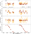 |
Fig. 1 NIRPS GTO data. The upper panel shows the nightly binned RV data of NIRPS and HARPS, obtained by the NIRPS GTO. The uppermiddle panel shows the time series of FWHM of the same spectra. The lower-middle panel shows the CRX data. The lower panel shows the BERV at which the measurements were taken. All data has its median value subtracted. |
2.6 Photometric data
The flux variations of Proxima have been intensively monitored over the years by various photometric surveys. We complemented the spectroscopic data with photometric time series obtained by the All Sky Automated Survey (ASAS; Pojmanski 1997), the All Sky Automated Survey for SuperNovae (ASAS-SN; Kochanek et al. 2017) and with data obtained using the Las Cumbres Observatory Global network (LCOGT, Brown et al. 2013). The full dataset consists of several thousands of epochs. To make it more manageable, we binned all photometric data every 2 days, resulting in 2212 binned measurements.
The ASAS data is composed of the observations taken by the ASAS-3 and ASAS-4 surveys. Both are V-band data taken over long baselines. We obtained the ASAS-3 data from the ASAS website2. The light curves include the photometric measurements obtained using four different apertures. We averaged over the four apertures to obtain the final photometric series, reducing the short-term scatter of the data. The ASAS-4 data was obtained from Damasso et al. (2020). The ASAS-4 data has error bars much larger than its short-term scatter. After an initial model, we concluded they are significantly over-estimated. For our analysis, we opted to scale them down to quarter. Even then, the excess white noise we measure remains comparable with the other photometric sources. The ASAS-3 data spans 8.7 years, between the years 2000 and 2009. It has an RMS of 33 ppt, and a median uncertainty of 13 ppt. The ASAS-4 data spans 8.8 years, between the years 2010 and 2019, with an RMS of 39 ppt, and a median uncertainty of 14 ppt.
The ASAS-SN data includes V -band and g-band data, taken between 2000-2007, and 2010-2024, respectively. We measured comparable RMS between the two. A preliminary photometric analysis showed indistinguishable behaviour between the two, which led us to combine the g-band data with the rest of the V-band data, to simplify the analysis. The V-band photometry has an RMS of 21.5 ppt, and a median uncertainty of 2.9 ppt. The g-band data has an RMS of 29.6 ppt, and a median uncertainty of 2.9 ppt.
There are two campaigns of V-band observations taken with the LCOGT. One obtained as support observations of the RedDots project, which were published alongside the original discovery of Proxima b (Anglada-Escudé et al. 2016). The other obtained as support observations of the ESPRESSO GTO, used in the confirmation of Proxima b with ESPRESSO (Suárez Mascareño et al. 2020). These campaigns produced time series with RMS of 23.0 ppt, and 10.59 ppt, respectively, and median uncertainties of 1.6 ppt, and 0.15 ppt, respectively.
The full photometric dataset can be found in Figure 2.
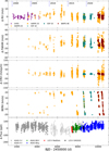 |
Fig. 2 All data. The upper panel shows the combined RV time series of Proxima. The upper-middle panel shows the time series of FWHM of the same spectra. The middle panel shows the CRX data. The lower-middle panel shows the BERV at which the measurements were taken. The lower panel shows the photometric data used in this work. |
RV data used in this work.
3 Properties of Proxima
Proxima, the closest star to the Sun, is one of the most well known stars. It is an M5.5 star, part of the triple system Alpha Centauri (Kervella et al. 2017). It has a mass of 0.12 M⊙ (Mann et al. 2015), a radius of 0.14 R⊙ (Boyajian et al. 2012), an effective temperature of 2900 K (Pavlenko et al. 2017), and a luminosity of 0.00151 ± 0.00008 L⊙ (Ribas et al. 2017). Using these values, we estimate the limits of the habitable zone (HZ) of the star to be 0.03731 ± 0.0075 au to 0.088 ± 0.017 au, following Kopparapu et al. (2014, 2017), for the runaway greenhouse to early-Mars limits. These limits correspond to orbital periods of 7.5 ± 2.2 days to 27.3 ± 7.8 days. From polarimetric measurements, Proxima’s rotation axis has been estimated to be tilted 47 ± 7° with respect to our line of sight (Klein et al. 2021). This value is reinforced by the report of a dust belt in the system, with a tilt of ~45°(Anglada et al. 2017). Table 2 shows the full list of parameters used in this study.
3.1 Magnetic cycle
Proxima is among the select group of fully convective M dwarfs with a known magnetic cycle. The cycle has been detected in photometry and X-ray (Suárez Mascareño et al. 2016; Wargelin et al. 2017), with a reported period be between 6.8 and 7.8 years, respectively. It has been reported to have an amplitude of 15-20 mmag in photometry, and its effects in RV and spectroscopic indicators have not been studied in-depth. More recently, Wargelin et al. (2024) re-analysed the photometric data, using a dataset very similar as the one used in this work, reporting a period of 7.99 ± 0.17 years.
Stellar properties of Proxima.
3.2 Rotation
Proxima rotates every 83-86 days, with variations easily detectable in photometry, spectroscopic indicators, and radial velocity. Wargelin et al. (2017) measured variations in these range of periods likely related to differential rotation. These rotational variations have been characterised many times over the years. The shape of the rotation curve is quite sinusoidal in photometry, with asymmetries that create some power at half the rotation period. Suárez Mascareño et al. (2020) showed that the relationship between the photometric and RV variations followed the concepts stated in Aigrain et al. (2012), with the activity-induced RV variations showing a good correlation with the gradient of the flux. The RV variations would often have the dominant signal at half the rotation period.
3.3 Planetary system
The planetary system of Proxima consists of one confirmed planet (Proxima b), and two candidates (Proxima c and d), that we know of.
Proxima b is an Earth-mass planet orbiting the habitable zone of the star. It has an orbital period of 11.1868 ± 0.0031 days, and a minimum mass of 1.07 ± 0.06 M⊕ (Faria et al. 2022). It was announced by Anglada-Escudé et al. (2016), using HARPS and UVES data, with the result being validated by Damasso & Del Sordo (2017). The planet was later independently confirmed by Suárez Mascareño et al. (2020), using ESPRESSO data. As it is one of the first terrestrial planets for which we expect to be able to survey the atmosphere, its potential habitability has been extensively discussed, with arguments in favour and against it (Ribas et al. 2016; Turbet et al. 2016; Dong et al. 2017; Howard et al. 2018; Meadows et al. 2018; Turbet et al. 2023).
Proxima c is a candidate long-period super-Earth. It was proposed by Damasso et al. (2020), after a re-analysis of the HARPS and UVES datasets. It orbits the star with a period of 1900 ± 96 days, and has a minimum mass of 5.8 ± 1.9 M⊕, A subsequent analysis of the HARPS data, using a different RV extraction method, could not find evidence of the presence of the planet (Artigau et al. 2022).
Proxima d is a candidate short-period sub-Earth. The presence of the signal was originally proposed by Suárez Mascareño et al. (2020), using ESPRESSO data, and solidified as a candidate by Faria et al. (2022), after an additional observation campaign. It orbits with a period of 5.122 ± 0.036 days and has a minimum mass of 0.26 ± 0.05 M⊕ (Faria et al. 2022).
4 Analysis
We performed a global analysis of the data, including always the full set of photometric data, along with spectroscopic activity proxies (FWHM and CRX), and the radial velocities. Both the spectroscopic proxy and the RV were separated between NIR and VIS data. Every time series includes a zero point per instrument, a model for the cycle, and a model for the stellar rotation. The cycle model is defined as a set of sinusoidal signals, with a common period and phase for all time series, and independent amplitudes. The stellar rotation is modelled as a multi-dimensional Gaussian Process. The RV data, in addition, includes polynomial terms against the CRX and BERV, and a circular or Keplerian model for each planet in the model.
We performed models that restricted the spectroscopic data to NIRPS, then models using the NIRPS and HARPS data from the NIRPS GTO, and models using the full spectroscopic dataset.
The full model is defined as
 (1)
(1)
where V0 represents the zero-point of each time series, with priors N[0, 100] ppt for the photometric data, N[0,40] ms−1 for the FWHM, and N[0, 10] ms−1 for the RVs. The rest of the components are described in the following subsections.
4.1 Cycle model
Based on the results of a photometric-only analysis (see Appendix A), and the test of the presence of the cycle in spectroscopic data (see Appendix B), the cycle component is defined as
 (2)
(2)

with t0 = 10 560 (BJD - 2 450 000) being the integer date of the last NIRPS observation. The cycle has independent amplitudes for photometry, FWHM, and RV. The photometry-only analysis revealed the length of the cycle to be much longer than previously thought (see Appendix A). Based on these results, the cycle period has a prior N [6400, 300] days. The phases have priors U[−0.5, 0.5]. The amplitudes in photometry are restricted to be positive (U[0, 50] ppt), while the amplitudes in FWHM and RV can be either positive or negative, to account for opposition of phase (N[0, 10] ms−1 for the FWHM, and N[0, 5] ms−1 for the RV).
This function will be applied to the photometric data, and to the visible-light FWHM and RV data, when using the complete dataset. In the case of the NIRPS data, the baseline of observations is too short to contribute to the determination of the cycle parameters (~600 days). The same is true for the HARPS data from the NIRPS GTO, when analysed alone. For the NIRPS data, and the HARPS data when restricted to the GTO observations, we simply account for a linear trend (Eq. (4)).
 (4)
(4)
with tmid = 10 264 (BJD - 2 450 000) being the mid-point of the NIRPS observing baseline. We set a prior N[0, 1] m s−1 d−1 for both the FWHM and RV slopes.
When analysing the NIRPS data together with the complete visible-light dataset, we will use a scaling factor of the complete visible-light model. We follow the formula
 (5)
(5)
where the scaling factor has a prior ln a U[−5, 3]. We assume the sign of the variations in NIR data to be the same as in the visible-light data.
Given the length of the cycle, and its shape, all models always include the full photometric dataset.
4.2 Stellar rotation model
To model the rotation we opted to work within the multidimensional Gaussian processes (GP) framework (Rajpaul et al. 2015). The GP framework has become the cornerstone method in the analysis of stellar activity in RV time series (e.g. Haywood et al. 2014). The stellar noise is described by a covariance with a prescribed functional form and the parameters attempt to describe the physical phenomena to be modelled. The GP framework can be used to characterise the activity signal without requiring a detailed knowledge of physical parameters of the underlying source of the variability. One of the biggest advantage of GPs is that they are flexible enough to effortlessly model quasi-periodic signals, and account for changes in the amplitude, phase, or even small changes in the period of the signal. This flexibility is also one of their biggest drawbacks, as they can easily overfit the data, suppressing potential planetary signals.
The multi-dimensional GP differs from the traditional 1D GP analysis by including the assumption that there exists an underlying function governing the behaviour of the stellar activity in all time series, which we denote G(t). G(t) manifests in each time series (Photometry, RV, etc.) as a linear combination of itself and its gradient, G′ (t), with a set of amplitudes for each time series, following the idea of the FF′ formalism (Aigrain et al. 2012), as described in Equation (6).
 (6)
(6)
with Δ TSi representing the variations of each time series, and Ai and Bi the scaling coefficients of the underlying function G(t) and its gradient, G′ (t), respectively.
The main advantage of the multi-dimensional GP over the traditional 1D GP, even if the parameters are trained in activity proxies, is the inclusion of all the data in the same covariance matrix. This imposes the behaviour of all time series to be correlated, rather than simply following qualitatively similar relationships.
We used the S+LEAF code (Delisle et al. 2022)3, which extends the formalism of semi-separable matrices introduced with celerite (Foreman-Mackey et al. 2017) to allow for fast evaluation of GP models even in the case of large datasets. This computational efficiency is key when evaluating datasets that include hundreds, or thousands, of measurements. The S+LEAF code supports a wide variety of GP kernels with fairly different properties. Based on the tests performed on the photometry-only model, we opted for a combination of two stochastic harmonic oscillators (SHO), one with a period equal to the rotation period, and the second at half the rotation period. This model resulted in the lowest amount of overfitting of long-period signals (see Appendix A). The kernel is defined as
 (7)
(7)
where k denotes the GP term, αi is the standard deviation of the process, Pi is the period of the oscillator, related to the rotation period, and Qi is the quality factor of the oscillator, related to the timescale of evolution L. These parameters are defined as
 (8)
(8)
Equation (7) also includes a term of uncorrelated noise (σ), independent for every instrument, added quadratically to the diagonal of the covariance matrix to account for all unmodelled sources of variation, such as uncorrected activity, instrumental instabilities, or additional planets. δτ is the Kronecker delta function, and τ represents a time interval between two measurements, t - t′. The white noise model uses log-normal priors, centred around the dispersion of the data and with a sigma similar to the dispersion of the data. This parametrisation makes it difficult for the model to converge to very low white noise values, while not forbidding them, which helps prevent overfitting. For the photometric data we used a prior ln σ N[3.5,3.5] (centred at −33 ppt), for the FWHM ln σ N[2.3,2.3] (−10 ms−1), and for the RVs ln σ N[0.5,0.5] (~1.65 ms−1). For the case of the RV data, this parametrisation makes it that deviating 3σ from the median value of the prior is equivalent to 37 cm s−1, and deviating 5σ corresponds to 14 cm s−1.
The amplitudes αi are related with the amplitude of the underlying function, not to any of the specific time series. These amplitudes are degenerate with the amplitudes of the component at each time series. We fixed them to 1, with the amplitudes of every component governed by the parameters Ai and Bi shown in Equation (6).
We used a prior N[85, 5] days for the rotation period, and a prior ln L U[3, 10] days for the timescale of evolution.
We used the photometric data as main dataset guiding the GP, which meant not including a gradient amplitude for it. The GP model, over all time series, is described as
 (9)
(9)
The scaling factor of the photometric component A1i have a prior U[0, 50]. The scaling factors of the FWHM and RV linear components Aii have priors U[−50, 50], while the scaling factors of the gradient components Bii have priors U[−100, 100].
4.3 Correlation with the chromatic index
The RV data of some of the instruments under study showed a correlation with the CRX (see Appendix C). Our initial tests found that this correlation survived the GP model and remained in the residuals. To account for this effect, we included a slope term between the RVs and the CRX, with different slopes for different instruments. Due to the lack of available activity indicators, the UVES data was not detrended.
The correlation takes the form of
 (10)
(10)
with a being the slope of the relationship, with a prior N[0, 0.3].
4.4 Correlation with the BERV
There are several effects potentially affecting the spectra, such as telluric contamination, ghosts, or CCD stitching, anchored at the detector reference frame (Dumusque et al. 2015; Coffinet et al. 2019; Cretignier et al. 2021). Combined with the movement of the Earth around the Sun, this results in periodic shifts with 1-year periodicity. All our spectra have been corrected from telluric contamination. However, there could be leftover effects which could still cause small RV shifts. To account for potential contamination, we included a polynomial term against the BERV (see Fig. 3 of Dumusque et al. 2015, and Appendix D). This term is defined as shown in Eq. (11), with different parameters for each instrument. Due to the lack of available data, the UVES data was not detrended.
The correlation takes the form of
 (11)
(11)
with a and b being the parameters of the polynomial, with priors N[0, 0.3].
4.5 Planetary model
All previously stated components of the model define our nullhypothesis model, meaning a model aimed to account for stellar activity and instrumental effects. On top of them, we include a planetary model where the number of planets will vary. The planetary signals are defined as circular for the detection tests, and later as full Keplerians to characterise their eccentricities. This choice avoids the potential pitfall of having a poorly sampled eccentric signal mimicking two circular signals and significantly cuts down on computing time.
RV variations due to circular planetary orbits are defined as
 (12)
(12)
where t0 = 10 560 + Ppl · (φpl - 1). This parametrisation ensures that our t0 coincides to the inferior conjunction of the planets, and is within the baseline of observations.
When conducting a blind search for planets, the orbital period is parametrised as angular frequency ω = 2π/Ppl. We use a prior U[2n/200, 2π/2] when analysing the NIRPS GTO data, as 200 days would be the largest period in which we could sample three full orbits. For the complete dataset, we use a prior U[2n/3000, 2π/2]. When performing a guided search using the published solutions, we directly sample the periods and use N priors centred around the published solution. The phases φpl are parametrised as U[−0.25, 0.75].
We parameterise the planetary amplitude K as ln K with a prior U[−5, 2] m s−1 (which keeps 50% of the prior space below 22 cm s−1). This parametrisation expands the parameter space around amplitudes consistent with zero, reducing potential biases towards large posteriors in noise dominated data, as described in Rajpaul et al. (2024).
RV variations due to planetary elliptical orbits are defined as
 (13)
(13)
where the true anomaly η is related to the solution of the Kepler equation, which depends on the orbital period of the planet Porb and the orbital phase φ. This phase corresponds to the periastron time, which depends on the mid-point transit time T0, the argument of periastron ω, and the eccentricity of the orbit e.
We parametrise  and
and  . We then sample
  and
and  with priors N[0, 0.3]. This parametrisation favours low eccentricities, which are expected for short-period signals.
The parameters of the planets are the same for the VIS and NIR time series.
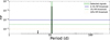 |
Fig. 3 FIP periodogram of the NIRPS-only model. The highlighted peak corresponds to the period of 11.19 days of Proxima b. |
4.6 Inference
We optimised the parameters of the models using Bayesian inference through the nested sampling (Skilling 2004, 2006) code Dynesty (Speagle 2020; Koposov et al. 2023).We sampled the parameter space using random slice sampling, which is well suited for the high-dimensional spaces (Handley et al. 2015a,b) resulting from modelling several time series at once. We used a number of live points of 20 × Nfree in models with narrow priors in period, and 100 × Nfree in models with wide priors, to ensure the discoverability of the narrow frequency posteriors.
5 Results
5.1 NIRPS-only RVs
The NIRPS GTO programme accumulated 149 nightly binned RV spectroscopic observations. The data spans a baseline of 604 days, with a median cadence of one visit per 1.1 nights (average one visit every 4.1 nights), corresponding with nightly observations with large gaps in between campaigns. The root mean square (RMS) of the RV data is of 1.69 m s−1, with a median uncertainty of55 cms−1. The RMS of the FWHM data is of 10.21 m s−1, with a median uncertainty of64 cm s−1. We analysed these data together with the complete photometric dataset, to guide the GP model.
We first performed a blind search of planetary signals. We used the model, as described in the previous section, with the spectroscopic data restricted to the NIRPS dataset. We include two planetary components in the model. Given the baseline of the observations, we do not attempt to survey the presence of Proxima c in the NIRPS data alone. We assessed the significance of the detection of the signals using the False inclusion probability (FIP) framework (Hara et al. 2022b). This framework uses the posterior distribution of the nested sampling run, and compute the probability of having a planet within a certain orbital frequency interval based on the relative weight of the samples within each frequency interval. The FIP framework has been demonstrated to minimise both false detections and missed detections, compared to other detection criteria such as the False Alarm Probability, or the Bayesian evidence. Based on an extensive set of simulations, Hara et al. (2022b) suggested an optimistic FIP threshold of 50%, that maximises detections, and a conservative threshold of 1%, that minimises false positives. Figure 3 shows the FIP periodogram of the data after analysing the posterior distribution of the two-planet model. The FIP periodogram shows the significant detection of a signal with a period of 11.19 days, corresponding to Proxima b, with a FIP < 0.001%, far below the conservative 1%. This strong detection supports the presence of Proxima b. There is an additional peak at 5.12 days, that passes the optimistic threshold but falls significantly short of the conservative threshold. This can be considered a tentative detection of the signal of Proxima d, or a hint of its presence in the data.
After the blind search, we perform a guided search, using the results obtained by Faria et al. (2022) as priors for the periods of the planetary signals. We use normal priors around the period of the solution of Faria et al. (2022), with a standard deviation of ~1% of the period. This corresponds to a prior N[11.1868,0.1] for Proxima b, and N[5.122, 0.05] for Proxima d. The priors for the RV amplitude and phase remain the same. We measure RV amplitudes of 1.15 ± 0.11 m s−1 for Proxima b, and 32 ± 14 cm s−1 for Proxima d, in complete agreement with the ESPRESSO results. The ephemerides of both are consistent with all previous publications. While not a formal detection, this is evidence of a signal consistent with the properties of Proxima d being present in the data. Figure 4 shows the model of the NIRPS RV, detrended from CRX, and of the FWHM data, along with their respective residuals, and Generalised Lomb-Scargle (GLS) periodograms (Zechmeister & Kürster 2009). The combination of the GP, the detrending, and planetary models accurately describes the variations in the data, leaving residuals with an RMS of 81 cm s−1, a 52% reduction with respect to the original data. In addition, the model accurately describes the variations in FWHM, which clearly show an ~80-day periodicity, linked to stellar rotation. The shape of the variations hints at the presence of several active regions, rotating at different rates. Figure 5 shows the phase-folded plots of the RV component caused by both planets.
Figure 6 shows a zoom to a section with high cadence observations taken at the beginning of the 2024 campaign. The model and the data show very good agreement. The visible variations are caused by the signals of Proxima b and d with the GP accounting only for low-frequency variations (timescales ~>40 days) linked to stellar rotation.
Regarding the stellar activity model, we measure the length of the stellar cycle to be 6425 ± 71 days, based entirely on the photometric data, with amplitudes of 34.0 ± 2.1 ppt, 5.0 ± 1.4 ppt, 5.7 ± 1.6 ppt, and 6.9 ± 1.3 ppt, at the components of Pcyc, Pcyc/2, Pcyc/3, and Pcyc/4, respectively. These results remain roughly consistent for all subsequent models (the timescales are dominated by the photometric data). We measure a stellar rotation period of 84.35 ± 0.90 days, with a timescale of evolution of 151 ± 41 days. The GP shows amplitudes of 20.8 ± 1.8 ppt, and 10.1 ± 1.2 ppt, at the components of Prot and Prot/2, respectively. We measure the variations in the FWHM to be anticorrelated with the variations in flux, and positively correlated with the gradient of the flux. The RV variations show a small positive correlation with the flux, and a large negative correlation with its gradient, but only for the component at Prot/2. The result is consistent with the expectations of spot-models (Aigrain et al. 2012). The activity model (trend against CRX and GP) account for an RMS of84 cms−1, while the polynomial against the BERV account for an RMS of 53 cm s−1. Figure D.1 shows these RV variations against the CRX and the BERV, along with the bestfit polynomial model. The variations correlated with the CRX are most likely caused by some form of activity of Proxima that is not fully captured by the photometry and FWHM, while those correlated with the BERV are likely the result of residual telluric contamination, detector defects, or other effects anchored in the detector reference frame.
As cross-check, we repeated the analysis using the LBL RVs derived from the spectra reduced with the ESO NIRPS DRS. We obtained very similar RVs, although noisier, and consistent results. The RV data from the NIRPS DRS showed an RMS of 2.11 ms−1, and we derived RV amplitudes of 1.00 ± 0.15 ms−1 for Proxima b, and 37 ± 20 cm s−1 for Proxima d. The results are in agreement with the ones obtained with spectra reduced with the APERO pipeline.
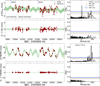 |
Fig. 4 Data and model of the NIRPS RV and DLW time series. The two top panels show the NIRPS RV data (detrended from CRX and BERV), with the best model fit (top; GP + two planets), and the residuals after the fit (bottom), along with the periodograms of both (right). The two bottom panels show the same for the FWHM. The shaded region shows the standard deviation of the GP model. |
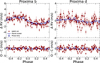 |
Fig. 5 NIRPS phase-folded plots of the planetary-induced RV signals. Left panels show the phase-folded RV variations induced by Proxima b (top), and the residuals after the fit (bottom). Right panels show the same for Proxima d. The blue hollow points represent the data binned by phase. |
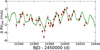 |
Fig. 6 Zoomed-in view of a high cadence RV campaign. NIRPS RV data of Proxima, detrended from CRX and BERV, along with the best model fit. The shaded region shows the standard deviation of the GP model. |
 |
Fig. 7 FIP Periodogram of the NIRPS+HARPS 2023-2024 model. The highlighted peak corresponds to the period of 11.19 days of Proxima b. The second weaker peak corresponds to 5.11 days, consistent with the period of Proxima d. |
5.2 Simultaneous HARPS data
After performing the model on the NIRPS data, we add the HARPS data obtained within the NIRPS GTO and repeat the models previously described. The HARPS RV data consists of 135 nightly binned epochs, over a baseline of 604 days, the same as the NIRPS data. The time series shows an RMS of 3.5 m s−1, with a typical measurement uncertainty of 1.4 m s−1.
Activity-induced RV variations of VIS and NIR data are expected to show different amplitudes (Carmona et al. 2023). We account for this effect by including different amplitudes for the GP component in the VIS and NIR data.
As in the NIRPS-only model, we first perform a blind search using the same period limits as before. The inclusion of the HARPS data does not change the significance of the detection of Proxima b, which was already nearly saturated with the NIRPS-only data. It, however, increases the significance of the peak corresponding to Proxima d, which rises up to a FIP of ~ 10% (see Fig. 7). This value of the FIP is in between the optimistic (50%) and conservative (1%) thresholds suggested by Hara et al. (2022b). It can be considered, at least, a tentative detection.
We repeat our guided search, with the same priors for the planets as before. With the combined GTO dataset we measure amplitudes of 1.198 ± 0.091 m s−1 for the signal of Proxima b, and 37.9 ± 9.9 cm s−1 for the signal of Proxima d. The signal at 5.12 days is detected at a >3-σ level. The ephemerides remain consistent. The residuals after the fit of the NIRPS data have an RMS of 0.84 ms−1, while those of HARPS are of 2.77 ms−1. Figure 8 shows the phase-folded plot of the HARPS+NIRPS RV variations of Proxima b and d.
We repeated both models using only the HARPS data from the NIRPS GTO. These data correspond to approximately the same baseline and exposure time as the NIRPS data, and can act as a good comparison of the performance of NIRPS. In the blind search, we did not have a significant detection of any signal. When performing the guided search, we measured an amplitude of 1.46 ± 0.31 ms−1 for Proxima b, and an amplitude <1.52 ms−1 (95% confidence) for Proxima d.
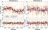 |
Fig. 8 Phase-folded plots of the planetary-induced RV signals in NIRPS and HARPS. Left panels show the phase-folded RV variations induced by Proxima b (top), and the residuals after the fit (bottom). Right panels show the same for Proxima d. |
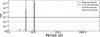 |
Fig. 9 FIP periodogram of the full dataset. The highlighted peaks corresponds to the period of 5.11 (Proxima d), and 11.19 (Proxima b). |
5.3 Full spectroscopic dataset
When including the full spectroscopic dataset, we construct a time series of 722 RV measurements, and 645 FWHM measurements, over a baseline of 24.5 years. The time series includes data of UVES, HARPS, ESPRESSO, and NIRPS. The RMS and median uncertainty of different time series is as follows: 2.00/0.64 m s−1 for UVES, 3.20/0.84 m s−1 for HARPS, 1.98/0.15 ms−1 for ESPRESSO, and 1.69/0.55 ms−1 for NIRPS. The combined dataset has an RMS of 2.67 m s−1, a median cadence of one point per 1.1 nights, and an average cadence of one point every twelve nights.
Following the same steps as with previous dataset, we start by performing a blind search. In this case, as the baseline is long enough, we test a four-planet model to account for the potential signal of the candidate Proxima c and an additional potential planetary signal present in the data. Figure 9 shows the FIP periodogram of the data, under the assumption of a model with up to four planets. We detect two significant peaks, at periods of 11.19 days, and 5.12 days, corresponding to the signals of Proxima b, and Proxima d. The detection of both signals is very significant, according to the FIP framework. Both peaks comfortably cross the 1% conservative threshold. In fact, the signals are present in virtually all the samples of the posterior distribution of the nested sampling run. We do not find additional significant peaks. There is one additional peak at 2.91 days, which does not reach the 10% FIP threshold. We investigated the posterior distribution to search for the presence, even marginal, of the signal of the candidate Proxima c. The combined posterior of the frequencies of the four planetary signals included in the model only has a few hundred samples (<0.1%) at periods within 3σ of the published period of Proxima c. We measure a period of 11.18482 ± 0.00028 days and an amplitude of 1.233 ± 0.037 ms−1 for Proxima b. For Proxima d, we measure a period of 5.12335 ± 0.00025 days and an amplitude of 36.8 ± 3.5 cms−1. We repeated the fit with a simpler three-planet model, with no significant changes.
Following the same steps as with previous datasets, and in an attempt to find the signal of the candidate Proxima c, we proceeded with a guided search. We set up a three-planets model. We maintained the priors of N [11.1868, 0.1] days for Proxima b, and N[5.122, 0.05] days for Proxima d, and used a prior N[1900, 200] days, following Damasso et al. (2020). We measure an RV semi-amplitude of 39.2 ± 5.5 cm s−1 for Proxima d, an orbital period of 5.12332 ± 0.00033 days, and a phase of 0.519 ± 0.031, which corresponds to a time of inferior conjuction Tc = 10557.54 ± 0.16 (BJD - 24 50 000). For Proxima b we measure an RV semi-amplitude of 1.234 ± 0.062 m s−1, an orbital period of 11.18472 ± 0.00051 days, and a phase of −0.020 ± 0.011, corresponding to a Tc = 10 548.59 ± 0.12 (BJD −2 450 000). We do not significantly detect the signal of Proxima c. We measure a semi-amplitude of 58 ± 28 cm s−1 (<1.4 ms−1, 99.7% confidence). We recover an orbital period of 1800 days, and a phase of 0.17
 , corresponding to a
  (BJD - 2 450 000). This hints at the presence of a long period signal with similar parameters, although not fully compatible, to those reported of the candidate Proxima c. Figure 10 shows the posterior distribution of the RV amplitude of the three signals.
As the cycle model could have an effect on the determination of the parameters of long-period planets, we repeated the three-planets model in the case of no-cycle model in RV, a simpler cycle model (1-sinusoidal), and a cycle model with a shorter period (following the results of Wargelin et al. (2024). All models provided upper limits to the presence of the signal consistent with that obtained using the default model.
From the two last models, we can confirm the detection of two signals, at periods of 5.123 days, 11.185 days. We cannot confirm the signal of the candidate Proxima c. However, we find hints of a long-period signal that might exists with not-too-different parameters. This signal, however, would have a significantly lower RV amplitude.
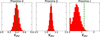 |
Fig. 10 RV amplitudes. Posterior distributions of the amplitudes of the RV signals. The vertical dashed lines show the previously reported amplitudes of Proxima d, b, and c. |
5.3.1 Stability of the detected signals
To test the stability of the planetary signals over time, we performed a new guided model on the two signals attributed to Proxima b and d, using apodised signals (Gregory 2016; Hara et al. 2022a). We define the apodised signals as:
 (14)
(14)
where G is Gaussian function with centre μ, width σ, and height 1. This model tests whether the intensity of the signal is uneven over the baseline of observations, and has proven effective in the past (Dumusque et al. 2017). As planetary signals are stable over time, we would expect to retrieve an undefined μ and a large σ. However, if we obtain a well-defined Gaussian, it would mean the signal is only present in part of the dataset. For this test, we used the same priors for the planetary parameters as stated before in the guided inferences. For the priors of the Gaussian, we used U[1634, 10560] (BJD - 2 450 000) for μ to cover the full baseline, and U[3, 15] for ln σ (20d to 3 × 10⁶ days), to allow for widths of the Gaussian much larger than the observation baseline, without biasing the results toward large widths.
The signals of Proxima b and d show strong stability, with a centre consistent with the full dataset, and median values of σ of 180 000 days, and 120 000 days, respectively. These values are much larger than the observing baseline.
Figure 11 shows the measured evolution of the amplitude over time. For Proxima b and Proxima d, the distribution is consistent with the final values of the global model throughout the complete baseline of observations. The range is wider at the beginning, coinciding with the data with the lowest observing cadence. Nevertheless, the signals are always present and remain at consistent amplitude with the median amplitude measured in the static model.
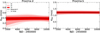 |
Fig. 11 Distribution of apodised amplitudes. The red shaded area shows the confidence intervals of the amplitudes of the apodised signals over time. The horizontal black lines show the median value and 1-σ range of the static model. |
5.3.2 Consistency between instruments
We performed a consistency test between the instruments by keeping the same global activity model and using independent sinusoidal signals for the planetary components in all the instruments. Since we do not expect all signals to be detectable in all instruments (e.g. Proxima d at 37 cm s−1), we kept the same priors of the guided search, with the aim of testing the differences in semi-amplitude and phase. For planetary signals, we expect all instruments to provide consistent results. For potential non-detections we expect to obtain upper limits that are consistent with the measurements in those instruments that provide a detection. Detections in a specific instrument, incompatible with upper limits from other instruments, would be indicative of instrumental effects.
Figure 12 shows the amplitude versus the time of inferior conjunction of the two signals for the different instruments. We found the properties of the signals of Proxima b and d to be consistent across all instruments. In the case of Proxima d, we find consistent parameter estimates in the data of ESPRESSO and HARPS. The amplitude measured in the HARPS data is slightly larger, but consistent within their respective confidence intervals. The constraints imposed by NIRPS and UVES are consistent with the measurement from ESPRESSO. These results are within the expectations of having a stable signal present in datasets of varying precision. In fact, the parameters obtained from all instruments are 1-σ compatible.
We performed one additional test of consistency between instruments. We compared the results obtained for Proxima d with ESPRESSO, against the results obtained using all other instruments combined. While these instruments, independently, struggled to provide a significant measurement, the combined dataset is capable of reaching it. Figure 12, right panel, shows the comparison between the parameters obtained with the ESPRESSO data, and those obtained by combining all other instruments. The parameters are fully consistent, showing that the presence and parameters of Proxima d are instrumentindependent.
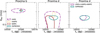 |
Fig. 12 Comparison of the parameters between instruments. RV semiamplitude vs. time of inferior conjunction for the solutions of individual instruments for Proxima b (left) and d (center). The right panel shows the same comparison for ESPRESSO-only and all other instruments combined. The lines encapsulate the 95% confidence interval. |
5.3.3 Adopted model
Following the results of Sections 5.3.1 and 5.3.2, we adopt a model that includes two sinusoidal signals to account for planets Proxima b and d. To establish the final parameters of these signals, we run a model using U priors for the periods, centred at the known period and with a range of ± 40% of the period. The rest of the priors for all parameters remain the same. We compared circular and Keplerian models and the results were consistent with each other. We measure eccentricities <0.1 for Proxima b and <0.25 for Proxima d (95% confidence). The rest of the parameters were consistent within 1σ. The circular model was statistically favoured, with a Δ ln Z = + 3 in favour of the simpler model. We adopt the circular model. The full set of priors and parameters of the adopted model is available in Appendix H.
We obtain parameters that are fully consistent with previous measurements. We measure Proxima b to have an orbital period of 11.18465 ± 0.00052 days and induce an RV semi-amplitude of 1.226 ± 0.062 ms−1. We measure a phase of −0.020 ± 0.011, which corresponds to a Tc = 10 548.59 ± 0.12 (BJD - 2 450 000). We measure Proxima d to have an orbital period of 5.12338 ± 0.00035 days and induce a semi-amplitude of 39.2 ± 5.7 cms−1. We measure a phase of 0.522 ± 0.031, which corresponds to a Tc = 10 557.55 ± 0.16 (BJD - 2 450 000).
Over the full dataset, we measure the stellar cycle to have a period of 6560 ± 85 days. It induces an RMS of 1.55 m s−1 in the FWHMVIS data and 0.56 m s−1 in the RVVIS data, with a peak-to-peak amplitude of 1.7ms−1. In the RVVIS, most of the detectable signal is present at half the cycle. We measure the stellar rotation period to be 83.2 ± 1.6 days, with a timescale of evolution of 60 ± 12 days. We measure an RV jitter of 57.5 ± 7.0 cm s−1 in the NIRPS data, 1.64 ± 0.21 m s−1 in the HARPS-03 data, 1.53 ± 0.12 m s−1 in the HARPS-15 data, 92 ± 21 cm s−1 in the UVES data, 42.5 ± 9.5 cm s−1 in the ESPRESSO-18 data, and 30.0 ± 7.0 cm s−1 in the ESPRESSO-19 data (95% confidence). The residuals after the fit do not highlight the presence of any significant periodic signal and show an RMS of 0.81 ms−1 in the NIRPS data, 1.51 ms−1 in the HARPS-03 data, 1.87 m s−1 in the HARPS-15 data, 0.59 m s−1 in the UVES data, and 0.20 m s−1 in the ESPRESSO data.
Figure 13 shows the full RV dataset, along with the bestfit model, the residuals, and their respective periodograms. Table G.1 shows the full set of priors, and the measured parameters, of the adopted model. Figure 14 provides a zoomed-in view of specific observing seasons. We separated the NIR and VIS data due to the different amplitudes of the activity model. Figure 15 shows the phase-folded plots of the planetary-induced RV signals. Appendix F contains the equivalent figures for the FWHM data and model.
6 Discussion
6.1 Performance of NIRPS
We studied the system of Proxima using the NIRPS spectrograph, while obtaining simultaneous HARPS spectra, providing us with a dataset in which NIRPS and HARPS share the same baseline, cadence, and exposure time. We measured the NIRPS data to have typical uncertainties of 55 cm s−1, compared to 1.4 m s−1 for the HARPS data. The NIRPS data showed a significantly lower RMS of 1.68 m s−1, compared to 3.54 m s−1 for HARPS. Most of this can be attributed to the significantly higher S/N data obtained with the NIRPS spectrograph at the same exposure time, while part of it can be ascribed to intrinsic instrumental stability. After modelling the combined GTO data (see Sect. 5.2), and subtracting the models, we measured an RMS of the residuals of 0.81 ms−1 in NIRPS, and 1.74 m s−1 for HARPS.
With this dataset, we provided a significant detection of Proxima b in the NIRPS dataset, while only a marginal detection in the HARPS data. Figure 16 shows the comparison of the amplitudes of the signals of Proxima b and d in the NIRPS, HARPS 2023-2024 data, the combined NIRPS+HARPS dataset, and the full spectroscopic dataset. Using the NIRPS data, we obtain a ~11-σ determination of the amplitude of Proxima b, which is accurate with the parameters obtained using ESPRESSO data. Using the HARPS 2023-2024 data, we achieved a ~4-σ determination. The combination of the two datasets reached a ~ 12-σ determination, and the full dataset a ~21-σ determination. In the case of Proxima d, the NIRPS dataset alone cannot provide a significant detection. Using the NIRPS data, we obtained a ~2-σ determination of the amplitude. Using the HARPS 2023-2024 data, we can barely reach ~1-σ determination. The combination of the two reached a ~4-σ determination, and the full dataset a ~7-σ determination. While the amplitude measurement of the signal in the NIRPS dataset cannot be considered significant, the peak of the posterior distribution is compatible with the posterior distribution obtained using the full dataset. In contrast, for the HARPS 2023-2024 dataset, the posterior distribution is mostly flat.
These results show that, in the case of Proxima, and at equal baseline and cumulative exposure time, NIRPS performs significantly better than HARPS. It would be expected that, with a larger dataset, NIRPS alone could be able to provide a fully independent detection of Proxima d, and the detection of other planetary signals inducing sub-m s−1 amplitude. It has to be said that, for the most recent dataset, the exposure time was optimised for NIRPS observations. Proxima is significantly brighter in the NIR than in the VIS, which permitted the use of shorter exposure times for the NIRPS observations. With longer exposure times it would be expected to obtain higher quality HARPS data.
Figure 17 shows the distribution of the RV residuals after the fit for all instruments, using the adopted model from Section 5.3.3. Here, once again, NIRPS compares favourably with HARPS. NIRPS residuals show an RMS of 80 cm s−1, comparable to UVES (80 cm s−1), which is mounted on an 8-meter telescope. HARPS shows residuals of 1.5 m s−1, while ESPRESSO stands on a league of its own, with just 20 cm s−1 residuals.
Parameters of the planets of the Proxima system, using the adopted model (circular).
6.2 The planetary system of Proxima
Our analysis provided significant detections of the signals of Proxima b and Proxima d. In the case of Proxima d, we provided significant evidence of the signal being present in spectrographs other than ESPRESSO and of its parameters being instrumentindependent. For the signals of Proxima b and d we found consistent parameters for parameters of the signal across the different models and instruments. We did not find conclusive evidence of the presence of the signal attributed to Proxima c in the data.
Table 3 shows the measured planetary parameters. The table provides updated ephemerides for the two planets in the system. Figure 15 shows the phase-folded RV data of two planetary signals.
6.2.1 Proxima b
Proxima b was announced using HARPS data (Anglada-Escudé et al. 2016) and later confirmed using ESPRESSO data (Suárez Mascareño et al. 2020). We confirm its presence once again using near-infrared radial velocities with NIRPS. We obtained a very significant detection within the FIP framework, as well as a measurement of its amplitude that is >10-σ different from zero. The planetary parameters derived from the NIRPS data are fully consistent with previous determinations.
Taking advantage of the complete dataset, we studied the temporal stability of the signal. We found its properties to be very consistent over the complete baseline of observations. Additionally, we demonstrated that the RV amplitude and phase obtained in the data of different instruments are consistent. We measure Proxima b to have an orbital period of 11.185 days, a minimum mass of 1.055 ± 0.055 M⊕, and an eccentricity lower than 0.1. It orbits at a distance of 0.04848 ± 0.00029 au and induces an RV amplitude of 1.226 ± 0.062 ms−1. With the complete dataset, we obtained ephemerides with a precision of 2.88 hours.
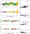 |
Fig. 13 RV model using the full dataset. The two top panels show the VIS RV data (detrended from CRX), with the best model fit (top), and the residuals after the fit (bottom), along with the periodograms of both (right). The two bottom panels show the same for the NIR RV data. |
6.2.2 Proxima d
The signal attributed to Proxima d was first discussed by Suárez Mascareño et al. (2020). The planet was later proposed as a candidate by Faria et al. (2022). Both works used ESPRESSO data. We provide a significant detection of Proxima d in our combined dataset, with parameters consistent with those proposed by Faria et al. (2022). In addition, we find strong evidence of the stability of the signal over time, and of its presence in instruments other than ESPRESSO. Our results confirm the presence of Proxima d, with an orbital period of 5.12338 ± 0.00035 days, a minimum mass of 0.260 ± 0.038 M⊕, and an eccentricity lower than 0.25. It orbits at a distance of 0.02881 ± 0.00017 au and induces an RV amplitude of 39.2 ± 5.7 cms−1. We provide ephemerides with a precision of 3.8 hours.
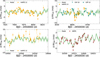 |
Fig. 14 Zoom to selected observing campaigns. RV data of HARPS, ESPRESSO, and NIRPS, detrended from CRX, with the best model fit. |
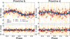 |
Fig. 15 Phase-folded plots of the planetary-induced RV signals. RV variations induced by Proxima b and d with the best model fit (top panels), and the residuals after the fit (bottom panels). The blue circles with white filling show the average at every phase bin. |
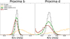 |
Fig. 16 Comparison of the amplitudes of NIRPS with other instruments. Posterior distributions of the RV amplitudes of Proxima b and d with NIRPS, HARPS, NIRPS+HARPS, and the full spectroscopic datasets. |
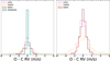 |
Fig. 17 Comparison of RV residuals. Distribution of the residuals of the RV data after subtracting the best fit. The left panel includes all instruments. The right panel excludes ESPRESSO, for an easier visualisation of the rest. |
6.2.3 Proxima c
Proxima c was proposed as a candidate by Damasso et al. (2020), but later challenged by Artigau et al. (2022). We attempted to detect the signal of Proxima c in our dataset but found no evidence of a significant signal within the FIP framework. In addition, we also did not find conclusive evidence when modelling the data using narrower priors around the period proposed by Damasso et al. (2020). We found hints of the presence of a signal at a similar period, but the amplitude and time of inferior conjunction were not consistent with those previously reported. By performing simple injection-recovery tests, we confirmed that we are sensitive to signals of 1 m s−1 amplitude at periods comparable to the proposed period of Proxima c.
6.2.4 Estimating the true masses of the planets
The rotation axis of Proxima has been estimated to be tilted 47 ± 7° with respect to our line of sight (Klein et al. 2021). In addition, Anglada et al. (2017) reported the detection ofa dust belt around the star, with a tilt angle of ~45°, which would make it coplanar to the rotation axis. Assuming the planetary orbits to be coplanar with the rotation axis, the masses of Proxima b, and d, would be 1.44 ± 0.21 M⊕, and 0.357 ± 0.072 M⊕, respectively.
6.2.5 Refinement of the planetary ephemeris
The planetary system of Proxima is one of the most promising candidates for the detection of atmosphere signatures in reflected light, or thermal emission, in rocky planets. It has been identified as a key target for RISTRETTO (Blind et al. 2022, 2024), ANDES (Palle et al. 2023) and LIFE (Quanz et al. 2022). Maintaining precise, and up-to-date, ephemeris of Proxima will be key to maximise the potential of detecting the planet signature and, potentially, information on the composition of its atmosphere. The addition of the NIRPS GTO data provides a significant improvement on the planetary ephemeris.
Using the previously publicly available data, we can measure the period of Proxima b with an uncertainty of 0.00076 days (65 seconds), and the time of inferior conjunction with an uncertainty of 0.16 days (3.8 hours). The addition of the NIRPS GTO data reduced the uncertainty in the period to 0.00053 days (46 seconds), and the uncertainty in the time of inferior conjunction to 0.12 days (2.9 hours). Moreover, the propagation of the uncertainty meant that a potential observation taken during 2026 would have had an uncertainty on the ephemeris of ~6 hours, which with the new data is reduced to ~3 hours.
In the case of Proxima d, with previously available data it was possible to constraint the period to an uncertainty of 0.0011 days (95 seconds), and the time of inferior conjunction to a precision of 0.26 days. With the NIRPS GTO data, we reduced the period uncertainty to 0.00035 days (30 seconds), and the time of inferior conjunction to 0.16 days (3.8 hours). A potential observation performed in 2026 would have had an uncertainty on the ephemeris of ~13.5 hours, that after the inclusion of the new data is reduced to −4 hours.
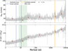 |
Fig. 18 Compatibility limits. The upper panel shows the RV amplitude limit (99%) as a function of orbital period. The blue shaded bars show the periods of the confirmed planets, Proxima b and Proxima c. The orange shaded line shows the period of the candidate Proxima c. The green shaded area shows the habitable zone. The red points shows those cases in which we obtained a >3 σ determination of the RV amplitude. The lower panels shows the same, but for planetary masses. |
6.2.6 Compatibility limits
Using the results from the adopted model on the full dataset, we measured the compatibility limits at a wide range of orbital periods of Proxima. We froze most of the parameters of the model (trends, cycle, GP, planets) and left free only the white noise and zero point RV components. We included a third sinusoid in the model, with only two parameters, RV amplitude and phase (parametrised as before). We fixed the orbital period to the period we wanted to test. This reduced the model to 12 parameters (five jitters, five zero-points, two sine parameters), which could be evaluated in a few seconds. Then randomly swept over the full range of orbital periods (1-10 000 days). From the posterior distribution of each try, we computed the 99% upper limit in RV amplitude, its median value, and standard deviation. Figure 18 shows these 99% RV limits as a function of orbital period, both in RV amplitude, and transformed to planetary mass. In addition, it shows the few cases in which the median value of the RV amplitude was more than 3-σ different from zero. We found that, for periods shorter than 10 days, we can exclude the presence of any additional signal with an amplitude larger than 20 cms−1 (minimum masses 0.08-0.15 M⊕). Within the habitable zone, we can exclude, for the most part, the presence of signals with amplitudes between 20 and 30 cm s−1 (m sin i 0.1-0.3 M⊕). At periods between the edge of the habitable zone (30d) and 100 days, we can exclude the presence of additional signals beyond 30-40 cm s−1 (m sin i 0.3-0.6 M⊕). Between 100 and 1000 days, the limit remains similar (0.51.0 M⊕). Beyond 1000-day orbital period, the limits raise up to ~60 cm s−1 (~4 M⊕).
While we did not formally detect the signal of Proxima c in our previous analysis (we only found an upper limit on a guided model), there is an RV amplitude excess at the period of the candidate consistent with the upper limit we previously measured. There seems to be an RV signal around 2000 days orbital period. This signal, however, needs to be of significantly lower amplitude than reported by Damasso et al. (2020). Our limit here is somewhat lower than what we derived when running a full three-planet model. This is likely due to the activity model changing to accommodate the signal in the case of the full model. In this case, the cycle model is fully frozen and, while the GP shape can still change slightly, its parameters cannot.
We encountered a few situations in which we measured amplitudes more than 3-σ different from zero. These signals have periods of 2.91d, 13.6d, 33d, 186d, 2000d, and 5350d. Their amplitudes are 18 cms−1, 12 cm s−1, 25 cms−1, 26 cms−1, 27 cm s−1, and 40 cm s−1, respectively. None of these were detected under a rigorous detection exercise. However, they could serve as hints that could guide future studies. The 2.91 d in particular coincides with a low-level peak in the FIP periodogram of the full dataset (see Figure 9).
6.3 Stellar activity
In conjunction with the planetary model, we characterised the activity variations of Proxima. We modelled the magnetic cycle in photometry, its induced variations in the width of the spectral lines, and the RV-induced variations. We modelled the stellar rotation, using multi-dimensional Gaussian processes regression. We measured the amplitude of the variations induced in photometry, in the width of spectral lines, and in RV, including the difference in amplitude between the visible and near-infrared data.
6.3.1 Magnetic cycle
For a long time, fully convective M dwarfs (i.e., M3.5 and later) were believed to be unable to support the magnetic dynamos necessary to support magnetic cycles. In recent years, however, several fully convective M dwarfs have shown to have magnetic cycles of lengths comparable to the solar cycle (Suárez Mascareño et al. 2016). In particular, a 7-8 year magnetic cycle was identified in Proxima using long-term photometric monitoring and X-ray data Jason et al. (2007); Suárez Mascareño et al. (2016); Wargelin et al. (2017, 2024).
For this work, we combined ground-based photometric data spanning 23.7 years of observations. The analysis of our data suggests the cycle is significantly longer than previously thought. Assuming we have observed the full cycle, we obtain a measurement of its length of 17.96 ± 0.23 years (6560 ± 85 days). The photometric variations due to the cycle are of −100 ppt peak-to-peak, comparable to those caused by the stellar rotation. This suggests that the change in the number of spots is not as significant as in a star like the Sun. Even at its quietest phase, the surface of Proxima maintains enough spot coverage to create −100 ppt peak-to-peak variations. The shape of the cycle is non-sinusoidal, which creates power at several of the harmonics of the main period. We modelled it as a combination of four sinu-soidals, with periods Pcycle,Pcycle/2, Pcycle/3, and Pcycle/4. This asymmetry, combined with the shorter baseline of observations used in previous works, likely explains most previous estimates.
While the parameters obtained in the fit are well constrained, and the model is visually compelling, the short baseline of the data compared to the measured period makes it difficult to be sure that this is the true period of the cycle. The results of Figure 20 hint at this period being at least close to the true period, by showing that the evolution of the photometric period shows a solar-like evolution when phase-folded with this cycle period. However, the difference between a cycle of 18 years and a cycle of half the period combined with a longer-term non-periodic variation is not obvious to disentangle with our dataset. The continuation of the photometric monitoring over the next decades will be crucial to confirm the true period of Proxima’s cycle.
By modelling the cycle simultaneously in photometry, FWHM, and RV, we can compare its signature in all of them. Figure 19 shows the cycle models in flux, FWHM, and RV, scaled to their own RMS. We find that the cycle in photometry and FWHM behaves in a very similar way, with only small differences in its shape. The opposition in sign shows that when the star becomes brighter, the line width becomes narrower, which is consistent with a spot-dominated stellar surface. In the case of the RV, the variations are somewhat more abrupt than in photometry or FWHM, with even a sign change when the slope of the flux variations changes at around BJD ~ 5000.
The measured period is approximately twice as long as the one measured by Wargelin et al. (2024), using a very similar photometric dataset. The difference between the two periods arises from differences in data treatment and modelling assumptions. By performing a source-by-source detrending, and assuming a simpler cycle model, we are able to reproduce their results. In our analysis, however, the inclusion of the spectroscopic data reinforces the push towards the longer period. With the current data, it is difficult to firmly establish which of the two sets of assumptions provide a more accurate result. Confidently disentangling the two scenarios would require a longer baseline of photometric and spectroscopic observations.
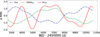 |
Fig. 19 Comparison of the cycle models. Cycle model in Flux, FWHM, and RV, showing the relationship between the components. |
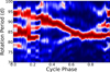 |
Fig. 20 Evolution of differential rotation. Colour map of the evolution of the periodogram power at different periods as a function of the cycle phase. The red shaded regions corresponds to the periods of high periodogram power. The blue shaded regions to the regions of low periodogram power. |
6.3.2 Differential rotation
Stars are not rigid bodies, which means not every part of their surface rotates at the same speed. This effect is primarily driven by the turbulent convection currents within the star. As hot plasma moves from the core to the surface, it carries angular momentum, resulting in different rates of rotation at different latitudes (Spruit 2002). Typically, the angular velocity decreases with increasing latitude, but that is not the case for all stars (Kitchatinov & Rüdiger 2004). In the case of the Sun, over the solar cycle, spots appear at high latitudes at the beginning of the cycle, migrating later to the equator as the cycle progresses. In photometry, this latitudinal movement corresponds to a slower rotation period at the beginning of the cycle that gradually increases until the end, before suddenly slowing down again. Wargelin et al. (2017) showed evidence of differential rotation in Proxima. However, the incompleteness of the data made it difficult to fully characterise its evolution.
Using the photometric data detrended from the magnetic cycle, with the parameters obtained from the full global model that included all available data, we attempted to measure variations in the photometric period. We computed a sliding periodogram over the data using a 2000 days window, using a frequency grid between 70 and 100 days. Figure 20 shows the map of the periodogram power as a function of the phase of the photometric cycle. We find that the photometric period varies smoothly as the cycle progresses, with a progression that resembles the butterfly diagram of the Sun. We measured multiple periods, between 83 and 95 days, at the beginning of the cycle, when the star is fainter. As the star becomes brighter, only the longer period survives, and it smoothly decreases until stabilising at ~83 days for the last third of the cycle. With these data, we measure a fractional rate of differential rotation of 0.16.
The evolution of the photometric rotation period resembles that of the Sun, with active regions appearing at high latitudes and then migrating towards more equatorial regions as the cycle progresses. However, it is important to remain cautious interpreting the data. The available time series cover less than two periodicities of the cycle, making it difficult to accurately phasefold the data. The conclusion is based on photometric flux, rather than number of spots present in the disk, which makes it difficult to establish the true beginning of the cycle. In addition, we do not know the inclination of the system. A pole-on stellar alignment might hide the variations related to equatorial spots.
We attempted the same exercise phase-folding with the period measured by Wargelin et al. (2024). In this case we did not find a coherent evolution over the cycle phase. We interpret this as evidence of the cycle being closer to 18 years.
6.3.3 Chromatic variations
We measured the stellar rotation-induced RV signal of Proxima to have a very small difference in amplitude between the visible and near-infrared data. The rotation variations in HARPS RV data taken simultaneously with the NIRPS data showed an RMS of 1.3 ms−1, compared to an RMS of 1.2 ms−1 in the nearinfrared data. Figure 21 shows the activity component of the RV data in HARPS and NIRPS overplotted. The shape of the variations is slightly different, with some sections in opposition of phase (BJD ~ 10 170), and others in phase (BJD ~ 10 550). The NIR data shows a clear peak in the periodogram close to the measured rotation period, while the VIS data shows a more complex pattern. The difference in RV amplitude is smaller than what might be expected when extrapolating from past results on active stars (Carmona et al. 2023). However, the activity-induced variations of Proxima are much smaller than those of any star when significant chromatic effects have been demonstrated. The results we obtain are closer to those of Cortés-Zuleta et al. (2023), which found that the stellar activity variations of Gl 205 in the visible and near-infrared are very similar in amplitude, although not necessarily in shape.
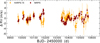 |
Fig. 21 Activity-induced RV variations. Activity-induced RV data from NIRPS and HARPS, after subtracting all planetary and instrumental effects. |
6.3.4 Differential temperature variations
Artigau et al. (2024) introduced a measurement of the differential change in effective temperature, based on small changes in the profile of stellar lines in high resolution spectroscopy, as part of the LBL framework (Artigau et al. 2022). We computed this differential temperature (dTEMP) for the NIRPS data, finding a typical variation of 2.11 K RMS, with a median uncertainty of 0.12 K. The variations show a very stable pattern following the rotation of the star. We compared them with the variations seen in photometry, FWHM, and RVs, corrected from planetary signals. Figure 22 shows the comparison of these data, all of them scaled to their own RMS. The dTEMP variations show a very similar pattern to the photometric variations, with the same periodicity and almost the exact same shape. At higher temperature we see the star becoming brighter, both implying a smaller filling factor. For Proxima, the dTEMP works as a very direct proxy of stellar flux. Compared to the FWHM, the dTEMP variations are in opposition, but still showing a very similar pattern. This emphasises that the PSF of NIRPS is stable enough that its changes are dominated by stellar variability. As in the case of ESPRESSO, NIRPS FWHM variations work as an inverse proxy of stellar flux (Suárez Mascareño et al. 2020). The activity-induced variations in RV follow these variations in dTEMP with the same periodicity, although the shape is slightly different. The RV variations seem to show a smaller slope over a rotation cycle. However, they are also noisier, making the comparison a bit more difficult. We modelled the dTEMP variation using the same GP-Kernel as used throughout the article. Figure 23 shows the best-fit model, and the residuals after the fit. We recovered similar parameters, although with larger parameter uncertainties, likely due to the lower amount of data. The residuals after the fit show an RMS of 0.25 K.
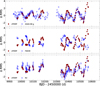 |
Fig. 22 Scaled dTEMP variations, compared to other activity proxies. The top panel shows the variations of the dTEMP compared to the variations in photometric flux. The middle panel shows the variations of the dTEMP compared to the variations in the FWHM. The bottom panel shows the variations of the dTEMP compared to the variations in the RV. All data and errors are scaled to the respective RMS of the displayed time series. |
7 Conclusions
We analysed the NIRPS RV data of Proxima, acquired within the context of the NIRPS GTO, the simultaneously obtained HARPS data, and the complete spectroscopic historical dataset spanning 24.5 years of observations. We complemented our analysis with 23.7 years of archival ground-based photometry. We performed a joint model that combined information from photometry, the variations in the width of stellar lines, RVs, variations in the chromatic RV slope, and BERV, into the multi-dimensional Gaussian process framework.
NIRPS provided an independent detection of Proxima b and evidence for Proxima d. The parameters obtained for Proxima b are consistent with previous studies, and the amplitude of the signal is constrained at a 10-σ level. The residuals after subtracting the best-fit model are ~80 cms−1, and show that NIRPS outperforms HARPS in RV precision for at least M6-type stars. Combining NIRPS and HARPS data improved detection significance and parameter precision, demonstrating their capability to detect Earth-mass planets around low-mass stars.
The full dataset confirmed Proxima b and d with extremely high confidence (FIP < 0.001%). Proxima b has a period of 11.18465 ± 0.00053 days, an RV amplitude of 1.226 ± 0.062 m s−1, and a minimum mass of 1.055 ± 0.055 M⊕. Proxima d has a period of 5.12338 ± 0.00035 days, an RV amplitude of 39.2 ± 5.7 cm s−1, and a minimum mass of 0.260 ± 0.038 M⊕, consistent with previous findings. Combining these results with previous measurements of the system inclination, and assuming coplanarity, we estimate that the true masses of Proxima b, and d, could be 1.44 ± 0.21 M⊕, and 0.357 ± 0.072 M⊕, respectively. No conclusive evidence was found for Proxima c, though hints of a lower-amplitude signal with a similar period exist. Taking advantage of the complete dataset, we demonstrate that the parameters of Proxima b and d are consistent between instruments, wavelengths, and over time.
We established compatibility limits for the presence of additional planets in the system. We exclude the presence of planets more massive than m sin i ~ 0.15 M⊕ at periods shorter than 10 days, more massive than 0.3 M⊕ in the habitable zone, 0.6 M⊕ up to 100 days, 1.0 M⊕ up to 1000 days, and to 4 M⊕ up to 10 000 days. Some RV excess at specific periods may warrant further study.
Using 23.7 years of ground-based photometric data, we updated the measurement Proxima’s magnetic cycle. We measure a length of 17.73 ± 0.22 years. The cycle shows significant asymmetries, which create power at several of its harmonics when modelling it by a combination of sine functions. The star’s photometric rotation period varies over the cycle, suggesting solar-like differential rotation.
We observe a very small chromatic effect in the activity-induced RV signal of Proxima. The RMS of the activity-induced RVs is ~10% larger in the contemporary HARPS dataset, compared to the NIRPS data.
Last, we find that the newly introduced dTEMP metric correlates well with flux and FWHM measurements, highlighting its potential as an activity proxy.
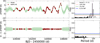 |
Fig. 23 NIRPS dTEMP model. The top row shows the NIRPS dTEMP data, along with the best fit model, and the GLS periodogram of the data. The lower row shows the residuals after the fit, along with their periodogram. |
Data availability
The data used in this paper is available at the CDS via anonymous ftp to cdsarc.cds.unistra.fr (130.79.128.5) or via https://cdsarc.cds.unistra.fr/viz-bin/cat/J/A+A/700/A11
Acknowledgements
We would like to thank Steve Saar, and Erik Mamajek, for useful discussion on Proxima’s stellar cycle, and its stellar parameters, respectively. ASM, JIGH, AKS, RR, FGT, NN, VMP & JLR acknowledge financial support from the Spanish Ministry of Science, Innovation and Universities (MICIU) projects PID2020-117493GB-I00 and PID2023-149982NB-I00. ÉA, NJC, RD, TV, CC, PLam, FBa, BB, LMa, RA, LB, AB, AD-B, LD, AL, OL, LMo, JS-A, PV & JPW acknowledge the financial support of the FRQ-NT through the Centre de recherche en astrophysique du Québec as well as the support from the Trottier Family Foundation and the Trottier Institute for Research on Exoplanets. ÉA, RD, FBa, LMa, TA, J-SM, MO, JS-A & PV acknowledges support from Canada Foundation for Innovation (CFI) program, the Université de Montréal and Université Laval, the Canada Economic Development (CED) program and the Ministere of Economy, Innovation and Energy (MEIE). XDe, XB, ACar, TF & VY acknowledge funding from the French ANR under contract number ANR18CE310019 (SPlaSH), and the French National Research Agency in the framework of the Investissements d’Avenir program (ANR-15-IDEX-02), through the funding of the “Origin of Life” project of the Grenoble-Alpes University. TV acknowledges support from the Fonds de recherche du Québec (FRQ) - Secteur Nature et technologies under file 320056. The Board of Observational and Instrumental Astronomy (NAOS) at the Federal University of Rio Grande do Norte’s research activities are supported by continuous grants from the Brazilian funding agency CNPq. This study was partially funded by the Coordenação de Aperfeiçoamento de Pessoal de Nível Superior—Brasil (CAPES) — Finance Code 001 and the CAPES-Print program. ICL acknowledges CNPq research fellowships (Grant No. 313103/2022-4). AKS acknowledges financial support from La Caixa Foundation (ID 100010434) under the grant LCF/BQ/DI23/11990071. SCB, ED-M, NCS, EC, ARCS & JGd acknowledge the support from FCT - Fundaçâo para a Ciência e a Tecnologia through national funds by these grants: UIDB/04434/2020, UIDP/04434/2020. SCB acknowledges the support from Fundaçâo para a Ciência e Tecnologia (FCT) in the form of a work contract through the Scientific Employment Incentive program with reference 2023.06687.CEECIND. BLCM & AMM acknowledge CAPES postdoctoral fellowships. BLCM acknowledges CNPq research fellowships (Grant No. 305804/2022-7). NBC acknowledges support from an NSERC Discovery Grant, a Canada Research Chair, and an Arthur B. McDonald Fellowship, and thanks the Trottier Space Institute for its financial support and dynamic intellectual environment. DBF acknowledges financial support from the Brazilian agency CNPq-PQ (Grant No. 305566/2021-0). Continuous grants from the Brazilian agency CNPq support the STELLAR TEAM of the Federal University of Ceara’s research activities. JRM acknowledges CNPq research fellowships (Grant No. 308928/2019-9). ED-M further acknowledges the support from FCT through Stimulus FCT contract 2021.01294.CEECIND. ED-M acknowledges the support by the Ramón y Cajal grant RyC2022-035854-I funded by MICIU/AEI/10.13039/501100011033 and by ESF+. XDu acknowledges the support from the European Research Council (ERC) under the European Union’s Horizon 2020 research and innovation programme (grant agreement SCORE No. 851555) and from the Swiss National Science Foundation under the grant SPECTRE (No. 200021_215200). This work has been carried out within the framework of the NCCR PlanetS supported by the Swiss National Science Foundation under grants 51NF40_182901 and 51NF40_205606. DE acknowledge support from the Swiss National Science Foundation for project 200021_200726. The authors acknowledge the financial support of the SNSF. CMo acknowledges the funding from the Swiss National Science Foundation under grant 200021_204847 “PlanetsInTime”. Co-funded by the European Union (ERC, FIERCE, 101052347). Views and opinions expressed are however those of the author(s) only and do not necessarily reflect those of the European Union or the European Research Council. Neither the European Union nor the granting authority can be held responsible for them. RA acknowledges the Swiss National Science Foundation (SNSF) support under the Post-Doc Mobility grant P500PT_222212 and the support of the Institut Trottier de Recherche sur les Exoplanètes (IREx). LB acknowledges the support of the Natural Sciences and Engineering Research Council of Canada (NSERC). This project has received funding from the European Research Council (ERC) under the European Union’s Horizon 2020 research and innovation programme (project Spice Dune, grant agreement No. 947634). This material reflects only the authors’ views and the Commission is not liable for any use that may be made of the information contained therein. ARCS acknowledges the support from Fundaçao para a Ciência e a Tecnologia (FCT) through the fellowship 2021.07856.BD. LD acknowledges the support of the Natural Sciences and Engineering Research Council of Canada (NSERC) and from the Fonds de recherche du Québec (FRQ) - Secteur Nature et technologies. FG acknowledges support from the Fonds de recherche du Québec (FRQ) - Secteur Nature et technologies under file 350366. HJH acknowledges funding from eSSENCE (grant number eSSENCE@LU 9:3), the Swedish National Research Council (project number 2023-05307), The Crafoord foundation and the Royal Physiographic Society of Lund, through The Fund of the Walter Gyllenberg Foundation. AL acknowledges support from the Fonds de recherche du Québec (FRQ) - Secteur Nature et technologies under file 349961. LMo acknowledges the support of the Natural Sciences and Engineering Research Council of Canada (NSERC), [funding reference number 589653]. NN acknowledges financial support by Light Bridges S.L, Las Palmas de Gran Canaria. NN acknowledges funding from Light Bridges for the Doctoral Thesis “Habitable Earth-like planets with ESPRESSO and NIRPS”, in cooperation with the Instituto de Astrofísica de Canarias, and the use of Indefeasible Computer Rights (ICR) being commissioned at the ASTRO POC project in the Island of Tenerife, Canary Islands (Spain). The ICR-ASTRONOMY used for his research was provided by Light Bridges in cooperation with Hewlett Packard Enterprise (HPE). CPi acknowledges support from the NSERC Vanier scholarship, and the Trottier Family Foundation. CPi also acknowledges support from the E. Margaret Burbidge Prize Postdoctoral Fellowship from the Brinson Foundation. This work is based on data obtained via the public archive at the European Southern Observatory (ESO). We are grateful to all the observers of the following ESO projects, whose data we are using: 072.C-0488, 082.C-0718, 183.C-0437, 191.C-0505, 096.C-0082, 099.C-0205, 099.C-0880, and 1102.C-0339. We are grateful to the crews at the ESO observatories of Paranal and La Silla. This research has made extensive use of the SIMBAD database, operated at CDS, Strasbourg, France, and NASA’s Astrophysics Data System. This research has made use of the NASA Exoplanet Archive, which is operated by the California Institute of Technology, under contract with the National Aeronautics and Space Administration under the Exoplanet Exploration Program. This work makes use of observations from the LCOGT network. The manuscript was written using VS Code. Main analysis performed in Python3 (Van Rossum & Drake 2009) running on Ubuntu (Sobell 2015) systems and MS. Windows running the Windows subsystem for Linux (WLS). Extensive use of the DACE platform4 Extensive usage of Numpy (van der Walt et al. 2011). Extensive usage of Scipy (Virtanen et al. 2020). AstroimageJ (Collins et al. 2017). TAPIR (Jensen 2013). All figures built with Matplotlib (Hunter 2007). The bulk of the analysis was performed on desktop PC with an AMD RyzenTM 9 9950X (16 cores, 32 threads, 3.5-4.7 GHz), provided by ASM, and a server hosting 2x AMD EpycTM 7663 (56 cores, 112 threads, per cpu), provided by the SUBSTELLAR ERC AdG.
Appendix A Photometric-only model
We analysed the photometric data to determine the best model for the cycle and the stellar rotation. We tested several different combinations of polynomials and sinusoidals, until converging to the sum of four sinusoidal signals at periods Pcycle, Pcycle/2, Pcycle/3, and Pcycle/4. Table A.1 shows the comparison of the parameters obtained, and the Bayesian evidence (Δ Log Z), of models using up to five sinusoidals. The model with four sinusoidals is preferred (Δ Log Z > 25 with respect to a single sinusoidal), and all the associated amplitudes are significantly measured. Figure A.1 shows the best-fit model, the residuals, and the periodograms of both. Models of lower complexity would leave residual signals with the period of the harmonics of the cycle. The periodogram of the data shows a dominant peak at 6400 days, with the periodogram of the residuals showing a peak at 83 days, corresponding to the stellar rotation.
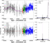 |
Fig. A.1 Cycle model. Photometric data with the best-fit model for the cycle, and the residuals after the fit. The right panels show the periodogram of the data and of the residuals. The horizontal lines in the periodograms show the 10% (red), 1% (green), and 0.1% (blue) false alarm probability thresholds. |
We modelled the stellar rotation using Gaussian process regression. We tested different kernels, including several combinations of stochastic harmonic oscillators (SHO), and variations of the Quasi-periodic (QP) kernel. We tried S+LEAF’s MEP, ESP, and ESP with additional harmonic components. We found that all the variations of the QP would supress the cycle signal. The same would happen with combinations of three SHO kernels, or more. A single SHO kernel would leave large residuals at the harmonics of the stellar rotation. The combination of two SHO kernels, centred at Prot, and Prot/2, provided a fit that both preserved the amplitudes of the cycle and its harmonic components, and suppressed the rotation signal. We opted for this last case to ensure that the GP model of choice would preserve, as much as possible, the presence of signals at periods longer than the stellar rotation (e.g long-period planets in the RV). We performed a blind determination of the cycle period and rotation periods, using Nested Sampling. We used a prior U[2000, 8000] for the cycle, and U[20, 200] for the stellar rotation. The best-fit model converted to a cycle period of 6425 ± 65 days, and a rotation period of 85 ± 1 days. We used these results, and the five times their uncertainties, as priors in all global models (N [6400,300] days for the cycle, N [85,5] days for the rotation). Figure A.2 shows the full model, combining the cycle and the GP components.
Comparison of cycle complexities
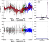 |
Fig. A.2 Full photometric model. Photometric data with the best-fit model combining cycle and rotation, and the residuals after the fit. The right panels show the periodogram of the data and of the residuals. |
Appendix B Presence of the cycle in spectroscopic data
Fig. B.1 shows the periodogram of the raw photometric, FWHM, and RV data. The zero-points of the individual datasets have been calculated by matching the median value of contemporary, or nearby, data. The periodograms show peaks, or power excesses, at long periods. These peaks, although poorly defined, are at periods between 5000 and 7000 days. Their origin might be tied to the same cycle seen in photometry. In addition, the periodogram of the FWHM shows several significant peaks (false alarm probability < 0.01) at shorter periods (108d, 270d, 1100d). These peaks correspond to 360d, 120d, and 90d, aliases of the rotation signal. To evaluate the importance of including a model for the stellar cycle in the spectroscopic data, we built a model using the full dataset (photometry, FWHM, and RV) that included all components described in section 4, except the planetary signals and the cycle model in spectroscopic data. We compared the change of the Bayesian evidence of the models after including the cycle model in FWHM, and then in RV.
We found that including the cycle model in FWHM was favoured (Δ LogZ ~ 7), compared to a model in which the cycle only affected the photometric data. We measured a significant amplitude at the main period of the cycle (7.3 ± 1.8 m s−1). For the FWHM, the variations at the harmonic components were not significant. Adding a cycle model in RV is once again favoured against the photometric-only model (Δ LogZ ~ 16) and against the model with the cycle in photometry and FWHM (Δ LogZ ~ 9). The signal in RV shows significant amplitudes at the main mode (0.86 ± 0.37 m s−1), the third harmonic (1.0 ± 0.25 m s−1) and the fourth harmonic (0.77 ± 0.21 m s−1). In all cases, the measured period remained consistent with the period of the photometry-only model.
With these results, we decided to include the cycle model both in FWHM and RV, following the same approach of the photometric cycle.
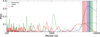 |
Fig. B.1 GLS periodogram of the photometric and spectroscopic data. Comparison of the periodograms of the photometric time-series, FWHM, and RV, focused on long periods. The shaded regions show the region of the highest periodogram power at periods longer than 2000 days. |
Appendix C Correlation with the chromatic index
Most RV data shows a significant trend against the chromatic index. The trend in all cases is positive. Figure C.1 shows the RV data of the three instruments against their respective CRX.
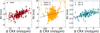 |
Fig. C.1 RV measurements against CRX. RV data of NIRPS, HARPS, and ESPRESSO, as a function of the chromatic index. The blue dotted line shows the best linear fit. |
Appendix D Correlation with BERV
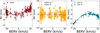 |
Fig. D.1 RV measurements against BERV. RV data of NIRPS, HARPS, and ESPRESSO, as a function of the barycentric earth radial velocity. The blue dotted line shows the best linear fit. |
Appendix E Detection of long period signals
We could not confirm the detection of the signal attributed to Proxima c. We could only measure an upper limit of the RV amplitude at the proposed period. To evaluate whether this is an indication that the signal does not exists in the data, or of the activity model is suppressing low-frequency signals, we performed simple injection-recovery tests. We conducted two tests in which we injected a long-period signal around the expected period of Proxima c. The injected signals were placed far enough apart that, if the signal of Proxima c exists, it should not interfere significantly with the injected signals. Additionally, the injected periods did not correspond to any harmonics of the stellar cycle. We tested one signal with shorter period (1400 days) and another one with a longer period (2400 days), both with RV amplitudes of 1 ms−1 and a Tc = 9000 (BJD - 2450000). We performed a guided search with the exact same setup as before, using priors of N[1400, 100] days, and N[2400, 200] days. In the first case, we recovered a period of 1418 ± 19 days, a semi-amplitude of 1.17 ± 0.20 ms−1, and a Tc = 9030 ± 50 (BJD - 2450000). In the second case, we recovered a period of 2407 ± 57 days, a semi-amplitude of 1.25 ± 0.32 ms−1, and a Tc = 8990 ± 95 (BJD - 2450000). With all recovered parameters being 1-σ accurate with those injected, it shows we would expect to detect a signal of 1 m s−1 at these periods.
Appendix F Adopted model - FWHM
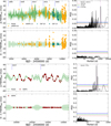 |
Fig. F.1 FWHM model using the full dataset. The two top panels show the VIS FWHM data, with the best model fit (top), and the residuals after the fit (bottom), along with the periodograms of both (right). The two bottom panels show the same for the NIR FWHM data. |
Appendix G Parameters of the adopted model
Priors and measured parameters of the adopted model.
Appendix H No transits in the TESS data
Since the discovery of Proxima b, there have been several attempts at detecting one of its transits. Jenkins et al. (2019) first reported a non-detection, using Spitzer observations. Later, Gilbert et al. (2021) reported the same using data from the first available TESS (Ricker et al. 2015) sectors. Using the four TESS sectors currently available (11, 12, 38, and 65) we repeat the exercise to confirm whether it is possible to detect a transit of Proxima b, or Proxima d, in the data. Following (Stefanov et al. 2025), we downloaded the light curves processed by the Science Processing Operations Center (SPOC) pipeline (Jenkins et al. 2016). We took all 2 min SAP measurements from all four sectors, using the hard cadence quality bitmask. Then, we smoothed the time series of each sector independently with the Tukey’s biweight time-window slider (Mosteller & Tukey 1977) through the Wotan library (Hippke et al. 2019). We used a window length of 6 h, a break tolerance of 12 h and no edge cut-offs. After detrending each sector individually and then combining them together, we could find no evidence of transits. Figure H.1, left panel, shows the phase-folded plot of the detrended TESS photometry, along with the expected transit signatures of both planets, for different impact parameters. Figure H.1, right panel, shows the time series of the detrended TESS photometry, with the dates of the expected transits highlighted. To this date, TESS has observed during eight potential transit dates of Proxima b, and 21 of Proxima d. In addition, we analysed the data looking for potential transit events with a period of 2.91d, as that signal appears both in the FIP periodogram from both Sects. 5.3 and 6.2.6. We did not find any event consistent with this period.
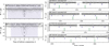 |
Fig. H.1 Phase-folded TESS data. Left panel shows the detrended SAP photometry folded with the periods, and ephemerides, of Proxima d (top panel), and Proxima b (bottom panel), with the expected transit signatures for different impact parameters. The shaded region shows the uncertainty in the ephemeris. Right panel shows the TESS SAP flux of the four available sectors, with the dates and predicted depths of the potential transiting events highlighted. The green horizontal lines, and shaded regions, mark the potential transits of Proxima b. The lilac lines, and shaded regions, mark the confidence interval of the potential transits of Proxima d. |
Appendix I Effect of changing the GP Kernel
In addition to the combination of two SHO kernels at PRot, and PRot/2, as presented through all the text, we re-run the adopted model using a single SHO (PRot), three SHOs (PRot, PRot/2, and PRot/4), the MEP kernel, the ESP kernel, and the ESP kernel with four harmonic components. The MEP and ESP Kernels are approximations of the traditional Quasi-Periodic kernel, written in the form of semi-separable matrices for increased computation efficiency (see Delisle et al. 2022). Except for the case of the single SHO, which would significantly underfit the data, the results of the parameters of planets b and d were consistent (within 1σ) in all cases. The biggest difference when using the combination of three SHOs, or the MEP/ESP kernels, was that they would suppress most low-frequency variations, independently of their origin. The most obvious effect would be in a reduction of the measured amplitude of the cycle, as the GP would absorbe part of that variation and to incorporate it into its own shape.
References
- Aigrain, S., Pont, F., & Zucker, S. 2012, MNRAS, 419, 3147 [NASA ADS] [CrossRef] [Google Scholar]
- Anglada, G., Amado, P. J., Ortiz, J. L., et al. 2017, ApJ, 850, L6 [Google Scholar]
- Anglada-Escudé, G., Amado, P. J., Barnes, J., et al. 2016, Nature, 536, 437 [Google Scholar]
- Artigau, É., Cadieux, C., Cook, N. J., et al. 2022, AJ, 164, 84 [NASA ADS] [CrossRef] [Google Scholar]
- Artigau, É., Bouchy, F., Doyon, R., et al. 2024, SPIE Conf. Ser., 13096, 130960C [Google Scholar]
- Bessell, M. S. 1991, AJ, 101, 662 [Google Scholar]
- Blind, N., Chazelas, B., Kühn, J., et al. 2022, SPIE Conf. Ser., 12185, 1218573 [NASA ADS] [Google Scholar]
- Blind, N., Shinde, M., Dinis, I., et al. 2024, SPIE Conf. Ser., 13097, 130976U [Google Scholar]
- Bonfils, X., Delfosse, X., Udry, S., et al. 2013, A&A, 549, A109 [NASA ADS] [CrossRef] [EDP Sciences] [Google Scholar]
- Bouchy, F., Doyon, R., Pepe, F., et al. 2025, A&A, 700, A10 [NASA ADS] [CrossRef] [EDP Sciences] [Google Scholar]
- Boyajian, T. S., von Braun, K., van Belle, G., et al. 2012, ApJ, 757, 112 [Google Scholar]
- Brown, T. M., Baliber, N., Bianco, F. B., et al. 2013, PASP, 125, 1031 [Google Scholar]
- Butler, R. P., Jones, H. R. A., Feng, F., et al. 2019, AJ, 158, 251 [Google Scholar]
- Carmona, A., Delfosse, X., Bellotti, S., et al. 2023, A&A, 674, A110 [NASA ADS] [CrossRef] [EDP Sciences] [Google Scholar]
- Coffinet, A., Lovis, C., Dumusque, X., & Pepe, F. 2019, A&A, 629, A27 [NASA ADS] [CrossRef] [EDP Sciences] [Google Scholar]
- Collins, K. A., Kielkopf, J. F., Stassun, K. G., & Hessman, F. V. 2017, AJ, 153, 77 [Google Scholar]
- Cook, N. J., Artigau, É., Doyon, R., et al. 2022, PASP, 134, 114509 [NASA ADS] [CrossRef] [Google Scholar]
- Cortés-Zuleta, P., Boisse, I., Klein, B., et al. 2023, A&A, 673, A14 [CrossRef] [EDP Sciences] [Google Scholar]
- Cretignier, M., Dumusque, X., Hara, N. C., & Pepe, F. 2021, A&A, 653, A43 [NASA ADS] [CrossRef] [EDP Sciences] [Google Scholar]
- Damasso, M., & Del Sordo, F. 2017, A&A, 599, A126 [NASA ADS] [CrossRef] [EDP Sciences] [Google Scholar]
- Damasso, M., Del Sordo, F., Anglada-Escudé, G., et al. 2020, Sci. Adv., 6, eaax7467 [Google Scholar]
- Dekker, H., D’Odorico, S., Kaufer, A., Delabre, B., & Kotzlowski, H. 2000, SPIE Conf. Ser., 4008, 534 [Google Scholar]
- Delisle, J. B., Unger, N., Hara, N. C., & Ségransan, D. 2022, A&A, 659, A182 [NASA ADS] [CrossRef] [EDP Sciences] [Google Scholar]
- Donati, J. F., Kouach, D., Moutou, C., et al. 2020, MNRAS, 498, 5684 [Google Scholar]
- Dong, C., Lingam, M., Ma, Y., & Cohen, O. 2017, ApJ, 837, L26 [NASA ADS] [CrossRef] [Google Scholar]
- Dumusque, X. 2018, A&A, 620, A47 [NASA ADS] [CrossRef] [EDP Sciences] [Google Scholar]
- Dumusque, X., Pepe, F., Lovis, C., & Latham, D. W. 2015, ApJ, 808, 171 [NASA ADS] [CrossRef] [Google Scholar]
- Dumusque, X., Borsa, F., Damasso, M., et al. 2017, A&A, 598, A133 [NASA ADS] [CrossRef] [EDP Sciences] [Google Scholar]
- Faria, J. P., Suárez Mascareño, A., Figueira, P., et al. 2022, A&A, 658, A115 [NASA ADS] [CrossRef] [EDP Sciences] [Google Scholar]
- Figueira, P., Marmier, M., Bonfils, X., et al. 2010, A&A, 513, L8 [NASA ADS] [CrossRef] [EDP Sciences] [Google Scholar]
- Foreman-Mackey, D., Agol, E., Ambikasaran, S., & Angus, R. 2017, AJ, 154, 220 [Google Scholar]
- Gaia Collaboration (Brown, A. G. A., et al.) 2021, A&A, 649, A1 [NASA ADS] [CrossRef] [EDP Sciences] [Google Scholar]
- Gilbert, E. A., Barclay, T., Kruse, E., Quintana, E. V., & Walkowicz, L. M. 2021, Front. Astron. Space Sci., 8, 190 [NASA ADS] [CrossRef] [Google Scholar]
- Gregory, P. C. 2016, MNRAS, 458, 2604 [NASA ADS] [CrossRef] [Google Scholar]
- Handley, W. J., Hobson, M. P., & Lasenby, A. N. 2015a, MNRAS, 450, L61 [NASA ADS] [CrossRef] [Google Scholar]
- Handley, W. J., Hobson, M. P., & Lasenby, A. N. 2015b, MNRAS, 453, 4384 [Google Scholar]
- Hara, N. C., Delisle, J.-B., Unger, N., & Dumusque, X. 2022a, A&A, 658, A177 [NASA ADS] [CrossRef] [EDP Sciences] [Google Scholar]
- Hara, N. C., Unger, N., Delisle, J.-B., Díaz, R. F., & Ségransan, D. 2022b, A&A, 663, A14 [NASA ADS] [CrossRef] [EDP Sciences] [Google Scholar]
- Haywood, R. D., Collier Cameron, A., Queloz, D., et al. 2014, MNRAS, 443, 2517 [Google Scholar]
- Hippke, M., David, T. J., Mulders, G. D., & Heller, R. 2019, AJ, 158, 143 [Google Scholar]
- Howard, W. S., Tilley, M. A., Corbett, H., et al. 2018, ApJ, 860, L30 [Google Scholar]
- Huélamo, N., Figueira, P., Bonfils, X., et al. 2008, A&A, 489, L9 [NASA ADS] [CrossRef] [EDP Sciences] [Google Scholar]
- Hunter, J. D. 2007, Comput. Sci. Eng., 9, 90 [NASA ADS] [CrossRef] [Google Scholar]
- Innes, R. T. A. 1915, Circ. Union Observ. Johannesburg, 30, 235 [Google Scholar]
- Jao, W.-C., Henry, T. J., Subasavage, J. P., et al. 2014, AJ, 147, 21 [Google Scholar]
- Jason, M., Guinan, E., Engle, S., & Pojmanski, G. 2007, in American Astronomical Society Meeting Abstracts, 211, 103.11 [Google Scholar]
- Jenkins, J. M., Twicken, J. D., McCauliff, S., et al. 2016, SPIE Conf. Ser., 9913, 99133E [Google Scholar]
- Jenkins, J. S., Harrington, J., Challener, R. C., et al. 2019, MNRAS, 487, 268 [Google Scholar]
- Jensen, E. 2013, Tapir: A web interface for transit/eclipse observability, Astrophysics Source Code Library, [record ascl:1306.007] [Google Scholar]
- Kasper, M., Cerpa Urra, N., Pathak, P., et al. 2021, The Messenger, 182, 38 [Google Scholar]
- Kervella, P., Thévenin, F., & Lovis, C. 2017, A&A, 598, L7 [NASA ADS] [CrossRef] [EDP Sciences] [Google Scholar]
- Kitchatinov, L. L., & Rüdiger, G. 2004, Astron. Nachr., 325, 496 [NASA ADS] [CrossRef] [Google Scholar]
- Klein, B., Donati, J.-F., Hébrard, É. M., et al. 2021, MNRAS, 500, 1844 [Google Scholar]
- Kochanek, C. S., Shappee, B. J., Stanek, K. Z., et al. 2017, PASP, 129, 104502 [Google Scholar]
- Koposov, S., Speagle, J., Barbary, K., et al. 2023, https://doi.org/10.5281/zenodo.7832419 [Google Scholar]
- Kopparapu, R. K., Ramirez, R. M., SchottelKotte, J., et al. 2014, ApJ, 787, L29 [Google Scholar]
- Kopparapu, R. k., Wolf, E. T., Arney, G., et al. 2017, ApJ, 845, 5 [NASA ADS] [CrossRef] [Google Scholar]
- Lo Curto, G., Pepe, F., Avila, G., et al. 2015, The Messenger, 162, 9 [NASA ADS] [Google Scholar]
- Lovis, C., Snellen, I., Mouillet, D., et al. 2017, A&A, 599, A16 [NASA ADS] [CrossRef] [EDP Sciences] [Google Scholar]
- Mann, A. W., Feiden, G. A., Gaidos, E., Boyajian, T., & von Braun, K. 2015, ApJ, 804, 64 [Google Scholar]
- Marconi, A., Abreu, M., Adibekyan, V., et al. 2022, SPIE Conf. Ser., 12184, 1218424 [NASA ADS] [Google Scholar]
- Mayor, M., Pepe, F., Queloz, D., et al. 2003, The Messenger, 114, 20 [NASA ADS] [Google Scholar]
- Meadows, V. S., Arney, G. N., Schwieterman, E. W., et al. 2018, Astrobiology, 18, 133 [Google Scholar]
- Mosteller, F., & Tukey, J. W. 1977, Data analysis and regression. A second course in statistics, Addison-Wesley Series in Behavioral Science: Quantitative Methods, Reading (Mass.: Addison-Wesley) [Google Scholar]
- Palle, E., Biazzo, K., Bolmont, E., et al. 2023, arXiv e-prints, [arXiv:2311.17075] [Google Scholar]
- Pavlenko, Y., Suárez Mascareño, A., Rebolo, R., et al. 2017, A&A, 606, A49 [NASA ADS] [CrossRef] [EDP Sciences] [Google Scholar]
- Pepe, F., Cristiani, S., Rebolo, R., et al. 2021, A&A, 645, A96 [NASA ADS] [CrossRef] [EDP Sciences] [Google Scholar]
- Pojmanski, G. 1997, Acta Astron., 47, 467 [Google Scholar]
- Quanz, S. P., Ottiger, M., Fontanet, E., et al. 2022, A&A, 664, A21 [NASA ADS] [CrossRef] [EDP Sciences] [Google Scholar]
- Queloz, D., Henry, G. W., Sivan, J. P., et al. 2001, A&A, 379, 279 [NASA ADS] [CrossRef] [EDP Sciences] [Google Scholar]
- Rajpaul, V., Aigrain, S., Osborne, M. A., Reece, S., & Roberts, S. 2015, MNRAS, 452, 2269 [Google Scholar]
- Rajpaul, V. M., Barragán, O., & Zicher, N. 2024, MNRAS, 530, 4665 [Google Scholar]
- Reiners, A., Zechmeister, M., Caballero, J. A., et al. 2018, A&A, 612, A49 [NASA ADS] [CrossRef] [EDP Sciences] [Google Scholar]
- Ribas, I., Bolmont, E., Selsis, F., et al. 2016, A&A, 596, A111 [NASA ADS] [CrossRef] [EDP Sciences] [Google Scholar]
- Ribas, I., Gregg, M. D., Boyajian, T. S., & Bolmont, E. 2017, A&A, 603, A58 [NASA ADS] [CrossRef] [EDP Sciences] [Google Scholar]
- Ricker, G. R., Winn, J. N., Vanderspek, R., et al. 2015, J. Astron. Telesc. Instrum. Syst., 1, 014003 [Google Scholar]
- Robertson, P., Mahadevan, S., Endl, M., & Roy, A. 2014, Science, 345, 440 [Google Scholar]
- Skilling, J. 2004, in American Institute of Physics Conference Series, 735, Bayesian Inference and Maximum Entropy Methods in Science and Engineering: 24th International Workshop on Bayesian Inference and Maximum Entropy Methods in Science and Engineering, eds. R. Fischer, R. Preuss, & U. V. Toussaint, 395 [Google Scholar]
- Skilling, J. 2006, Bayesian Anal., 1, 833 [Google Scholar]
- Sobell, M. G. 2015, A Practical Guide to Ubuntu Linux (Pearson Education) [Google Scholar]
- Speagle, J. S. 2020, MNRAS, 493, 3132 [Google Scholar]
- Spruit, H. C. 2002, A&A, 381, 923 [CrossRef] [EDP Sciences] [Google Scholar]
- Stefanov, A. K., González Hernández, J. I., Suárez Mascareño, A., et al. 2025, A&A, 693, L3 [NASA ADS] [CrossRef] [EDP Sciences] [Google Scholar]
- Suárez Mascareño, A., Rebolo, R., & González Hernández, J. I. 2016, A&A, 595, A12 [Google Scholar]
- Suárez Mascareño, A., Rebolo, R., González Hernández, J. I., & Esposito, M. 2017, MNRAS, 468, 4772 [Google Scholar]
- Suárez Mascareño, A., Faria, J. P., Figueira, P., et al. 2020, A&A, 639, A77 [Google Scholar]
- Turbet, M., Leconte, J., Selsis, F., et al. 2016, A&A, 596, A112 [NASA ADS] [CrossRef] [EDP Sciences] [Google Scholar]
- Turbet, M., Fauchez, T. J., Leconte, J., et al. 2023, A&A, 679, A126 [NASA ADS] [CrossRef] [EDP Sciences] [Google Scholar]
- van der Walt, S., Colbert, S. C., & Varoquaux, G. 2011, Comput. Sci. Eng., 13, 22 [Google Scholar]
- Van Rossum, G., & Drake, F. L. 2009, Python 3 Reference Manual (Scotts Valley, CA: CreateSpace) [Google Scholar]
- Virtanen, P., Gommers, R., Oliphant, T. E., et al. 2020, Nat. Methods, 17, 261 [Google Scholar]
- Wargelin, B. J., Saar, S. H., Pojmanski, G., Drake, J. J., & Kashyap, V. L. 2017, MNRAS, 464, 3281 [NASA ADS] [CrossRef] [Google Scholar]
- Wargelin, B. J., Saar, S. H., Irving, Z. A., et al. 2024, ApJ, 977, 144 [Google Scholar]
- Wildi, F., Bouchy, F., Doyon, R., et al. 2022, SPIE Conf. Ser., 12184, 121841H [NASA ADS] [Google Scholar]
- Zechmeister, M., & Kürster, M. 2009, A&A, 496, 577 [CrossRef] [EDP Sciences] [Google Scholar]
- Zechmeister, M., Reiners, A., Amado, P. J., et al. 2018, A&A, 609, A12 [NASA ADS] [CrossRef] [EDP Sciences] [Google Scholar]
Version 0.65.001, https://lbl.exoplanets.ca.
All Tables
Parameters of the planets of the Proxima system, using the adopted model (circular).
All Figures
|
Fig. 1 NIRPS GTO data. The upper panel shows the nightly binned RV data of NIRPS and HARPS, obtained by the NIRPS GTO. The uppermiddle panel shows the time series of FWHM of the same spectra. The lower-middle panel shows the CRX data. The lower panel shows the BERV at which the measurements were taken. All data has its median value subtracted. |
| In the text | |
|
Fig. 2 All data. The upper panel shows the combined RV time series of Proxima. The upper-middle panel shows the time series of FWHM of the same spectra. The middle panel shows the CRX data. The lower-middle panel shows the BERV at which the measurements were taken. The lower panel shows the photometric data used in this work. |
| In the text | |
|
Fig. 3 FIP periodogram of the NIRPS-only model. The highlighted peak corresponds to the period of 11.19 days of Proxima b. |
| In the text | |
|
Fig. 4 Data and model of the NIRPS RV and DLW time series. The two top panels show the NIRPS RV data (detrended from CRX and BERV), with the best model fit (top; GP + two planets), and the residuals after the fit (bottom), along with the periodograms of both (right). The two bottom panels show the same for the FWHM. The shaded region shows the standard deviation of the GP model. |
| In the text | |
|
Fig. 5 NIRPS phase-folded plots of the planetary-induced RV signals. Left panels show the phase-folded RV variations induced by Proxima b (top), and the residuals after the fit (bottom). Right panels show the same for Proxima d. The blue hollow points represent the data binned by phase. |
| In the text | |
|
Fig. 6 Zoomed-in view of a high cadence RV campaign. NIRPS RV data of Proxima, detrended from CRX and BERV, along with the best model fit. The shaded region shows the standard deviation of the GP model. |
| In the text | |
|
Fig. 7 FIP Periodogram of the NIRPS+HARPS 2023-2024 model. The highlighted peak corresponds to the period of 11.19 days of Proxima b. The second weaker peak corresponds to 5.11 days, consistent with the period of Proxima d. |
| In the text | |
|
Fig. 8 Phase-folded plots of the planetary-induced RV signals in NIRPS and HARPS. Left panels show the phase-folded RV variations induced by Proxima b (top), and the residuals after the fit (bottom). Right panels show the same for Proxima d. |
| In the text | |
|
Fig. 9 FIP periodogram of the full dataset. The highlighted peaks corresponds to the period of 5.11 (Proxima d), and 11.19 (Proxima b). |
| In the text | |
|
Fig. 10 RV amplitudes. Posterior distributions of the amplitudes of the RV signals. The vertical dashed lines show the previously reported amplitudes of Proxima d, b, and c. |
| In the text | |
|
Fig. 11 Distribution of apodised amplitudes. The red shaded area shows the confidence intervals of the amplitudes of the apodised signals over time. The horizontal black lines show the median value and 1-σ range of the static model. |
| In the text | |
|
Fig. 12 Comparison of the parameters between instruments. RV semiamplitude vs. time of inferior conjunction for the solutions of individual instruments for Proxima b (left) and d (center). The right panel shows the same comparison for ESPRESSO-only and all other instruments combined. The lines encapsulate the 95% confidence interval. |
| In the text | |
|
Fig. 13 RV model using the full dataset. The two top panels show the VIS RV data (detrended from CRX), with the best model fit (top), and the residuals after the fit (bottom), along with the periodograms of both (right). The two bottom panels show the same for the NIR RV data. |
| In the text | |
|
Fig. 14 Zoom to selected observing campaigns. RV data of HARPS, ESPRESSO, and NIRPS, detrended from CRX, with the best model fit. |
| In the text | |
|
Fig. 15 Phase-folded plots of the planetary-induced RV signals. RV variations induced by Proxima b and d with the best model fit (top panels), and the residuals after the fit (bottom panels). The blue circles with white filling show the average at every phase bin. |
| In the text | |
|
Fig. 16 Comparison of the amplitudes of NIRPS with other instruments. Posterior distributions of the RV amplitudes of Proxima b and d with NIRPS, HARPS, NIRPS+HARPS, and the full spectroscopic datasets. |
| In the text | |
|
Fig. 17 Comparison of RV residuals. Distribution of the residuals of the RV data after subtracting the best fit. The left panel includes all instruments. The right panel excludes ESPRESSO, for an easier visualisation of the rest. |
| In the text | |
|
Fig. 18 Compatibility limits. The upper panel shows the RV amplitude limit (99%) as a function of orbital period. The blue shaded bars show the periods of the confirmed planets, Proxima b and Proxima c. The orange shaded line shows the period of the candidate Proxima c. The green shaded area shows the habitable zone. The red points shows those cases in which we obtained a >3 σ determination of the RV amplitude. The lower panels shows the same, but for planetary masses. |
| In the text | |
|
Fig. 19 Comparison of the cycle models. Cycle model in Flux, FWHM, and RV, showing the relationship between the components. |
| In the text | |
|
Fig. 20 Evolution of differential rotation. Colour map of the evolution of the periodogram power at different periods as a function of the cycle phase. The red shaded regions corresponds to the periods of high periodogram power. The blue shaded regions to the regions of low periodogram power. |
| In the text | |
|
Fig. 21 Activity-induced RV variations. Activity-induced RV data from NIRPS and HARPS, after subtracting all planetary and instrumental effects. |
| In the text | |
|
Fig. 22 Scaled dTEMP variations, compared to other activity proxies. The top panel shows the variations of the dTEMP compared to the variations in photometric flux. The middle panel shows the variations of the dTEMP compared to the variations in the FWHM. The bottom panel shows the variations of the dTEMP compared to the variations in the RV. All data and errors are scaled to the respective RMS of the displayed time series. |
| In the text | |
|
Fig. 23 NIRPS dTEMP model. The top row shows the NIRPS dTEMP data, along with the best fit model, and the GLS periodogram of the data. The lower row shows the residuals after the fit, along with their periodogram. |
| In the text | |
|
Fig. A.1 Cycle model. Photometric data with the best-fit model for the cycle, and the residuals after the fit. The right panels show the periodogram of the data and of the residuals. The horizontal lines in the periodograms show the 10% (red), 1% (green), and 0.1% (blue) false alarm probability thresholds. |
| In the text | |
|
Fig. A.2 Full photometric model. Photometric data with the best-fit model combining cycle and rotation, and the residuals after the fit. The right panels show the periodogram of the data and of the residuals. |
| In the text | |
|
Fig. B.1 GLS periodogram of the photometric and spectroscopic data. Comparison of the periodograms of the photometric time-series, FWHM, and RV, focused on long periods. The shaded regions show the region of the highest periodogram power at periods longer than 2000 days. |
| In the text | |
|
Fig. C.1 RV measurements against CRX. RV data of NIRPS, HARPS, and ESPRESSO, as a function of the chromatic index. The blue dotted line shows the best linear fit. |
| In the text | |
|
Fig. D.1 RV measurements against BERV. RV data of NIRPS, HARPS, and ESPRESSO, as a function of the barycentric earth radial velocity. The blue dotted line shows the best linear fit. |
| In the text | |
|
Fig. F.1 FWHM model using the full dataset. The two top panels show the VIS FWHM data, with the best model fit (top), and the residuals after the fit (bottom), along with the periodograms of both (right). The two bottom panels show the same for the NIR FWHM data. |
| In the text | |
|
Fig. H.1 Phase-folded TESS data. Left panel shows the detrended SAP photometry folded with the periods, and ephemerides, of Proxima d (top panel), and Proxima b (bottom panel), with the expected transit signatures for different impact parameters. The shaded region shows the uncertainty in the ephemeris. Right panel shows the TESS SAP flux of the four available sectors, with the dates and predicted depths of the potential transiting events highlighted. The green horizontal lines, and shaded regions, mark the potential transits of Proxima b. The lilac lines, and shaded regions, mark the confidence interval of the potential transits of Proxima d. |
| In the text | |
Current usage metrics show cumulative count of Article Views (full-text article views including HTML views, PDF and ePub downloads, according to the available data) and Abstracts Views on Vision4Press platform.
Data correspond to usage on the plateform after 2015. The current usage metrics is available 48-96 hours after online publication and is updated daily on week days.
Initial download of the metrics may take a while.