| Issue |
A&A
Volume 699, July 2025
|
|
|---|---|---|
| Article Number | A1 | |
| Number of page(s) | 21 | |
| Section | Cosmology (including clusters of galaxies) | |
| DOI | https://doi.org/10.1051/0004-6361/202453483 | |
| Published online | 25 June 2025 | |
The eventful life journey of galaxy clusters
I. Impact of dark matter halo and intracluster medium properties on their full assembly histories
1
Departament d’Astronomia i Astrofísica, Universitat de València, E-46100 Burjassot, (València), Spain
2
Observatori Astronòmic, Universitat de València, E-46980 Paterna, (València), Spain
⋆ Corresponding author: This email address is being protected from spambots. You need JavaScript enabled to view it.
Received:
17
December
2024
Accepted:
5
May
2025
Abstract
Context. Galaxy clusters assemble over gigayears in a very anisotropic environment, leading to a remarkable diversity in their mass assembly histories (MAHs).
Aims. In this work, we aim to understand how the present-day properties of the dark matter (DM) halo and the intracluster medium (ICM) are related to the whole evolution of these structures.
Methods. To this end, we analysed a ΛCDM hydrodynamical + N-Body simulation of a (100 h−1 Mpc)3 volume, containing over 30 clusters and 300 groups. We looked at the individual and the stacked MAHs (determined from complete merger trees) in relation to the properties of the DM halos and the ICM at a fixed cosmic time (i.e. indicators of assembly state).
Results. The ensemble MAHs are well separated when stacked in bins of these indicators, yielding clear dependencies of the evolutionary properties (e.g. formation redshift) on the fixed-time halo properties. Additionally, we find that different indicators offer a varying range of information on distinct epochs of accretion. Finally, by summarising the complex MAH diversity with two parameters, we have described how different indicators bring in complementary information in different directions of this biparametric space. Overall, the halo spin and a combined indicator appear to be the ones encoding the most information about the MAH.
Conclusions. The results shown here add up to the idea that the dynamical state of cosmic structures is a multifaceted concept, with a warning that single indicators are incapable of capturing the whole complexity of the process. This work sheds light on the nature of this characterisation by untangling precisely when and how a number of these indicators provide information about. In turn, these results offer clues that can help to better constrain the MAH of observed structures.
Key words: methods: numerical / methods: statistical / galaxies: clusters: general / galaxies: clusters: intracluster medium / galaxies: groups: general / large-scale structure of Universe
© The Authors 2025
 Open Access article, published by EDP Sciences, under the terms of the Creative Commons Attribution License (https://creativecommons.org/licenses/by/4.0), which permits unrestricted use, distribution, and reproduction in any medium, provided the original work is properly cited.
This article is published in open access under the Subscribe to Open model. This email address is being protected from spambots. You need JavaScript enabled to view it. to support open access publication.
1. Introduction
Galaxy clusters and groups, spanning a mass range from 1013 M⊙ to a few times 1015 M⊙, form through the most energetic (up to ∼1061 − 65 erg) and long-lasting (on timescales comparable to the Hubble time) events in the Universe (Kravtsov & Borgani 2012; Planelles et al. 2015). Within this process, dark matter (DM) and baryons collapse in an increasingly inhomogeneous and anisotropic environment, due to the emergence of an intricate web of filaments, walls, and voids (White et al. 1987; Bond et al. 1996). Additionally, the process is hierarchical and, thus, the mass growth of clusters is made possible by contributions resulting from the accretion of smooth material from the cosmic web as well as from a more intermittent and violent component associated to mergers of similarly-sized objects (Gott & Rees 1975; White & Rees 1978). All this complexity is imprinted in the high diversity of mass assembly histories (MAHs), where (even at fixed present-day mass), there is a very considerable scatter in M(z)/M0 (e.g. Maulbetsch et al. 2007; Zhao et al. 2009; Vallés-Pérez et al. 2020).
Characterising the formation history of galaxy clusters and groups is of utmost importance, since it has been linked to a plethora of properties and phenomena of the DM halo and of the intracluster medium (ICM). Regarding the latter, these include, for instance, turbulence (Dolag et al. 2005; Lau et al. 2009; Vazza et al. 2017; Vallés-Pérez et al. 2021) leading to mass bias (Lau et al. 2013; Nelson et al. 2014; Vazza et al. 2018; Angelinelli et al. 2020; Bennett & Sijacki 2022), self-similarity (or a lack thereof) when considering either integrated properties (McCarthy et al. 2008; Poole et al. 2008; Planelles & Quilis 2009; Chen et al. 2019) or radial profiles (Lau et al. 2015), ram-pressure stripping of infalling satellites (Lourenço et al. 2023), or gas clumping (Nagai & Lau 2011; Vazza et al. 2013; Eckert et al. 2015; Angelinelli et al. 2021). As per the properties of the DM halo, the splashback radius (More et al. 2015; Diemer et al. 2017; Pizzardo et al. 2024) and/or its shape (Gouin et al. 2021; Lau et al. 2021; Cataldi et al. 2023) have also been linked to its MAH.
However, most of these works correspond to numerical studies, where the whole evolutionary history of these structures can be explicitly followed. While there are recipes for the direct estimation of mass accretion rates (MARs) on actual observational data (e.g. Pizzardo et al. 2021, 2022; using the caustic technique under reasonable, simplifying assumptions, De Boni et al. 2016; as well as Soltis et al. 2025, who built a machine learning model based on multi-wavelength data), most often the assessment of the assembly state of galaxy clusters is done by looking at morphological and dynamical properties of either their radio, optical, or X-ray emission, or their Sunyaev-Zeldovich signal (e.g. Rasia et al. 2013; Lovisari et al. 2017; Zenteno et al. 2020; Campitiello et al. 2022; Biava et al. 2024).
At the same time, as of three decades ago, simulations have been helpful in our attempts to understand which properties of a cluster or its DM halo are most affected by its MAH. Simple quantities that can be derived from the three-dimensional (3D) description only available in simulations include the offset between any pair of definitions of the cluster centre (Crone et al. 1996; Macciò et al. 2007; Cui et al. 2016), the ratio of kinetic to gravitational energies (Shaw et al. 2006; Neto et al. 2007; Knebe & Power 2008; Cui et al. 2017), or the fraction of the total halo mass in sub-structures (Neto et al. 2007; or variants thereof; see e.g. Kimmig et al. 2023). More recently, other quantities have shown significant potential for constraining the evolutionary properties of DM halos, such as the halo concentration (Neto et al. 2007; Wang et al. 2020) or sparsity (Balmès et al. 2014; Corasaniti et al. 2018), amongst others. In addition, the thermodynamical state of the cluster core (in particular, ‘cool-cored-ness’, Rasia et al. 2015; Rossetti et al. 2017) and properties of the stellar component (e.g. ‘fossil-ness’, Ragagnin et al. 2019, or the fraction of mass in the brightest cluster galaxy and the intracluster light, Kimmig et al. 2025) have been extensively studied in relation to cluster assembly.
Even going beyond the intrinsic interest on this topic because of its implications for observational studies (e.g. sample selection, constraining assembly histories, etc.), the search for proxies for the dynamical state or the assembly information has been targeting growing interest lately, as it has been shown that this notion of dynamical state is multifaceted (Haggar et al. 2024; in the sense of being able to be split in several, more fundamental properties highlighting different distinct, uncorrelated features) and potentially time-dependent (Vallés-Pérez et al. 2023, hereon VP23; implying that the optimal combination of different indicators that best predicts the presence of assembly episodes is not constant through cosmic time, but, rather, is strongly evolving), where additionally the different properties under study tend to be only mildly correlated (Jeeson-Daniel et al. 2011; Skibba & Macciò 2011).
In this context, recent literature on the topic still lacks a comprehensive and systematic view regarding what specific part of the MAH of galaxy groups and clusters is each of the myriad of indicators informing about and how far it goes to constrain the MAH or the quantities derived from it. Wong & Taylor (2012) performed one of the first studies in this particular direction, using DM-only simulations to explore how the MAH of DM halos can be decomposed and what information the halo shape can yield on these components. In addition, Giocoli et al. (2012) described how the halo concentration depends, in a non-trivial way, on several epochs of the assembly history of the halo (i.e. on a combination of the times at which the halo had built 4% and 50% of its present-day mass). However, to our best knowledge, no study in the literature has taken a systematic look at the relation of DM halo morphological and dynamical parameters on instantaneous properties, such as accretion rates, and neither have accounted for the differences in ICM and DM quantities.
This is the first article of a series aimed at studying the effects of mass accretion onto simulated galaxy clusters and groups on their morphological, dynamical, thermodynamical, and observational properties. In this first paper, we aim to study in detail the precise information on the full MAH and the associated MARs is yielded by a number of properties of the DM halo and the ICM when measured at z = 0 (or at another, fix cosmic time). We want to constrain when, what, and to what extent each of these quantities contribute information in this context. In particular, the specific aims of this work have been to establish (i) the effect of selecting clusters based on their assembly state indicators on their ensemble MAHs; (ii) when mass accretion affects the value of each parameter at z = 0 the most; (iii) besides timing, what additional information on the MAH each parameter encodes; and (iv) how consistent these indicators are when measured from the DM distribution and from the ICM.
The paper is organised as follows. In Sect. 2, we describe the simulation data, our set of assembly state indicators, and the statistical treatment. Subsequently, in Sect. 3, we describe and discuss our results in relation to the four points above. Finally, Sect. 4 contains a summary of the main conclusions together with additional discussion and comparisons with the literature. Appendices A and B discuss, respectively, our strategy for building the merger trees along with its impact on our results, and a presentation of some of the more technical points regarding the principal component analysis (PCA) of the assembly histories.
2. Methods
The results in this paper stem from the analysis of a Lambda cold dark matter (ΛCDM) N-body + hydrodynamical simulation, whose technical details are covered in Sect. 2.1. The halo catalogues and merger trees, as well as the characterisation of their assembly state, are subsequently described in Sects. 2.2 and 2.3, respectively. In Sect. 2.4, we cover our determination of the assembly histories and accretion rates. Finally, Sect. 2.5 deals with several aspects of the statistical analyses in this work.
2.1. Simulation
We performed and analysed a cosmological ΛCDM simulation of a cubic domain of L = 100 h−1 cMpc on each side. The assumed background cosmology is specified by a dimensionless Hubble constant h ≡ H0/(100 km s−1 Mpc−1) = 0.678, matter and baryonic density parameters of Ωm = 0.31 and Ωb = 0.048, respectively, and a null spatial curvature (ΩΛ = 1 − Ωm) that is generally compatible with the results reported by Planck Collaboration VI (2020).
The initial conditions were generated from an unconstrained realisation of a primordial power spectrum with an index of ns = 0.96 and an amplitude yielding σ8 = 0.82, with a baryonic transfer function at z = 1000 (Eisenstein & Hu 1998), further evolved until zini = 100 under the Zel’dovich (1970) approximation. From zini until z = 0, the fully non-linear evolution is followed with the MASCLET code (Quilis 2004), which combines a Eulerian, high-resolution shock-capturing (HRSC) treatment of the equations of hydrodynamics and an N-body approach for DM based on the particle-mesh method, both within an adaptive mesh refinement (AMR) scheme, allowing for high dynamical ranges to be achieved.
The simulation was run with a base grid of Nx3 = 2563 cells and nℓini = 3 levels of refinement, already present on the initial conditions (equivalent to an effective 20483 resolution in dense regions). During the evolution, up to nℓ = 6 refinement levels are dynamically generated, with criteria based on overdensity (standard, pseudo-Lagrangian AMR), converging flows, and Jeans length. Overall, this gives a peak spatial resolution of Δx6 = 9 kpc and a peak DM mass resolution of MDM, peak = 1.5 × 10⁷ M⊙. Besides the hydrodynamical and gravitational forces, only cooling is included, but with no star formation or additional feedback mechanisms. Further details on this simulation are also covered by Vallés-Pérez et al. (2024).
Since this work is focused on large aperture radii (typically, R200m; see definition below), the lack of feedback mechanisms (which typically impact the inner radii, r ≲ (0.3 − 1)R500c, e.g. Duffy et al. 2010; Planelles et al. 2014, 2017) is unlikely to have a substantial qualitative contribution to our results. Masses (and, thus, MAHs) at R200m are minimally affected by feedback (e.g. Teyssier et al. 2011). Regarding cluster properties (such as those introduced below in Sect. 2.3), we note that while feedback could moderately impact their values, these are quantities integrated over a large (∼Rvir) aperture and should therefore remain relatively stable and be monotonically related to the equivalent quantities in the absence of feedback (albeit with considerable scatter; see, for instance, Corasaniti et al. 2025 for the case of sparsity).
2.2. Cluster catalogues and merger trees
Simulations were post-processed with the public halo finder ASOHF1 (Planelles & Quilis 2010; Knebe et al. 2011; Vallés-Pérez et al. 2022) to extract a catalogue of DM halos at each snapshot. Halos at different snapshots were connected using the ancillary mtree.py code of the ASOHF package, which determines all contributors to a halo in an (immediate or not) previous snapshot.
The catalogue of galaxy clusters and groups was then selected at z = 0 as a mass-limited sample, containing all objects with virial mass2MvirDM(z = 0) > 1013 M⊙, which are additionally sufficiently well-refined (at least up to ℓ = 4, Δx4 = 36 kpc) and away from the domain boundaries. The main branch of the merger tree was traced back in time down to z = 4 using a double-fold criterion looking the most gravitationally-bound particle in the progenitor and descendant halos (i.e. the most-bound particle in the progenitor is amongst the descendant particles and vice-versa; see Section 2.6.2 in Vallés-Pérez et al. 2022, as well as Appendix A in this work, for more details and discussion).
The resulting catalogue comprises 31 galaxy clusters, whose z = 0 virial mass exceeds 1014 M⊙, together with 358 groups (1013 < MvirDM/M⊙ < 1014). Regarding the completeness of the merger tree, 90% of the catalogue is traced back to at least z = 2. The fraction starts to decline more rapidly at higher redshift, with 80% at z = 3 and 50% at z ≳ 4. Unless where specified otherwise, the results have been obtained by considering the complete sample of clusters and groups.
2.3. Assembly state indicators
We aimed to study how the MAHs of our clusters and groups depend on several parameters of the DM (or the ICM) at given, fixed cosmic times. Many of these indicators were already introduced by VP23 in their study of the assembly state of DM halos, and are only summarised here for completeness.
-
Centre offset (Δr), defined as the distance between the DM density peak and the centre of mass in units of the virial radius,
 (e.g. Crone et al. 1996; Cole & Lacey 1996; Cui et al. 2016).
 -
Virial ratio (η), namely, the quotient between twice the kinetic and the gravitational binding energies, η ≡ 2T/|W|. While there are different choices as per whether to correct this quantity by a surface energy term (Poole et al. 2006; Shaw et al. 2006; Power et al. 2012), as discussed in VP23, we do not consider this correction, since it tends to erase the correlation with merging activity and would make this quantity less useful as an indicator of assembly state.
-
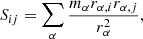
Mean radial velocity (
 ) of the dark matter particles, computed as
 (1)
(1)where mα and
 are, respectively, the mass and the radial velocity (in the halo reference frame) of the α-th particle, while
  is the circular velocity at the virial radius.
 -
Sparsity (s200c, 500c), which is the quotient between3M200c and M500c and provides similar information to halo concentration, albeit in a non-parametric way (Balmès et al. 2014; Corasaniti et al. 2018; Richardson & Corasaniti 2022).
-
Ellipticity (ϵ), computed from the reduced shape tensor,
 (2)
(2)whose eigenvalues λ1 ≥ λ2 ≥ λ3 are proportional to the semiaxes (a ≥ b ≥ c) squared, from which we define
 . This and other quantities relating to halo shape have been recently related to the assembly history of DM halos (e.g. Chen et al. 2019; Lau et al. 2021).
 -
Sub-structure fraction (fsub), namely, the quotient between the total mass in sub-structures (each delimited by its Jacobi radius; see e.g. Binney & Tremaine 1987) over the total, virial mass of the halo.
-
Spin parameter (λBullock), which is a normalised measure of the DM angular momentum in units of
 (Bullock et al. 2001).
 -
Combined relaxedness indicator (χ). Inspired by the functional form used by Haggar et al. (2020) and subsequent works, in VP23 we introduced a summary measure of relaxedness that takes into account the first six parameters in this list in a redshift-dependent combination. Formally, this is defined as
![Mathematical equation: $$ \begin{aligned} \chi = \left[ \sum _{i = 1}^6 w_i (z) \left( \frac{X_i}{X_i^\mathrm{thr} (z)}\right)^2\right]^{-1/2}, \end{aligned} $$](/articles/aa/full_html/2025/07/aa53483-24/aa53483-24-eq9.gif) (3)
(3)where Xi represents each of the six aforementioned parameters and the weights wi(z) and thresholds Xithr(z), which were calibrated as a function of redshift by VP23 and Vallés-Pérez (2024). In this definition, χ does not account for λBullock. While the methodology in VP23 admits introducing as many indicators as desired, λBullock was not considered in the calibration by Vallés-Pérez (2024). For the sake of conciseness, we chose to stick to the aforementioned calibration in this work. Since the parameters for χ were calibrated to correlate with merging activity, we do not expect the inclusion of additional indicators to substantially impact our results.
Each of these quantities (except for χ) is intuitively correlated with the notion of a dynamically active halo, which is undergoing significant assembly activity. All quantities are computed from the 3D description of the DM distribution and, unless otherwise stated (e.g. s200c, 500c), all bound particles within the virial radius are used in the computation.
2.4. Determination and stacking of the MAHs and MARs
The MAHs of the DM component for individual clusters and groups were determined by summing the masses of all bound DM particles within the spherical overdensity radius (e.g.4R200m) at each snapshot with redshift z, yielding M200mDM(z). For gas mass, M200mgas(z), we added the mass of all cells whose centre lies within a sphere of R200m. Here, treating cells as pointwise particles for the purpose of mass integration implies quasi-Poissonian errors of ∼1% or below for the largest mass objects (up to ∼3% for the lowest mass ones), which can be safely disregarded given the typical mass variations during the considered redshift interval of around 2 orders of magnitude. Note that we did not perform any unbinding for gas for simplicity, as baryons have already been shock-heated at distances much larger than the apertures we use and their velocity distribution does not exhibit the same high-velocity tails as DM.
The MAHs from a sub-sample of clusters (in terms of e.g. mass or any assembly state indicator) are stacked at each redshift by iteratively computing the biweight mean (i.e. robust mean; as e.g. described in Beers et al. 1990; Wilcox 2012) of the values of log10M(z)/M0. Missing data (either clusters that are lost in a particular snapshot and recovered afterwards, or clusters where the main branch of the merger tree is interrupted) were ignored in this calculation. Through the paper, we refer to two measures of the scatter around these MAHs:
-
Scatter around the MAH, computed from the 1σ confidence interval in log10M(z)/M0, where σ is determined as the robust standard deviation (or biweight midvariance; Wilcox 2012).
-
Uncertainty in determining the mean MAH (i.e. standard errors), computed by taking the standard deviation of the distribution of mean values obtained by bootstrap resampling.
Finally, the instantaneous MARs,
 (4)
(4)
are computed in a similar way to Vallés-Pérez et al. (2020), by resampling the M(a) by cubic interpolation in logarithmic space to a vector of values of the scale factor, a, which is logarithmically spaced with Δlog a = 0.01 dex. Then, we apply a Savitzky & Golay (1964) cubic filter to compute the derivatives with window length of 15 points (Δlog a = 0.15 dex), which roughly corresponds to a dynamical time. Thus, our Γ200m are instantaneous accretion rates smoothed over a dynamical time, to prevent the noisy behaviour of individual MAHs to contaminate the determination of the derivatives.
2.5. Partial correlations and directions of maximal variation
In different sections of the results, we make extensive reference to different correlation coefficients amongst the assembly state indicators and the MAHs or MARs. For clarity, we describe all of them in detail here.
2.5.1. Linear and non-linear partial correlations
In Sect. 3.2, we have aimed to establish the relation between MAHs or MARs and several properties of the cluster. Given that these quantities may have implicit dependencies with mass (see, e.g. Figs. 1 and 2 below), it is important to account for them so that we look at the correlations at fixed mass. While splitting objects in mass sub-samples could alleviate this problem, it would come at the cost of greatly reducing the sample sizes and thus the statistical power. Instead, we account for these dependences by using partial correlation coefficients (Cramer 1946), which account for the correlation between a pair of variables (namely, x and y) while fixing one or more additional quantities (z). If the correlations are assumed to be linear, this comes down to finding the linear relations x(z) and y(z) and determining the Pearson correlation coefficients of the residuals (ϵx)i = xi − x(zi) and (ϵy)i = yi − y(zi). This can be developed to derive a general expression for the partial correlation between x and y fixing z,
 (5)
(5)
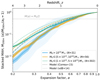 |
Fig. 1. Stacked mass assembly histories (MAHs) in three mass sub-samples, corresponding to galaxy clusters (light blue, thicker lines), high-mass groups (orange), and low-mass groups (turquoise, thinner lines). Dark shaded regions indicate the 1σ uncertainty around each mean MAH. Light shaded regions indicate the population standard deviation (just shown for the galaxy clusters sub-sample for clarity). Dashed (dotted) lines show the MAHs expected for each mass range according to the analytic (semi-analytic) model by Correa et al. (2015) (van den Bosch et al. 2014). |
 |
Fig. 2. Corner plot showing the univariate and bivariate distribution of the assembly state indicators and mass at R200m, all measured at z = 0. Along the diagonal, each panel presents the distribution of one variable, with the text in the top indicating the median value and (16, 84) percentiles. The sub-diagonal terms are scatter plots of the pair of variables indicated by the respective row and column. The text in magenta within each off-diagonal panel indicates the Spearman rank correlation coefficient between the corresponding pair of variables. The panels above the diagonal represent the same information as contours, for better visualisation in the densest parts. |
where ρAB is the regular Pearson correlation coefficient. Dropping the assumption of linearity, Pearson coefficients in Eq. (5) can be substituted by Spearman rank correlation coefficients5 if the relation is monotonic.
In other instances (e.g. Sect. 3.3.1), we have aimed at quantifying the ability of a third variable, z, to break the scatter between a pair of variables x and y with an unknown, possibly non-monotonic underlying relation. Being non-monotonic, the approach above (i.e. computing ρyz|x) is no longer valid. In these cases, we perform a non-parametric fit to the y = f(x) relation with smoothing cubic splines. In particular, we used the FITPACK implementation (Dierckx 1995), where the number of polynomials (the lower this number, the smoother the resulting interpolation) is set as the lowest fulfilling the condition
![Mathematical equation: $$ \begin{aligned} \sum _{i = 1}^N \frac{1}{\sigma (y_i)^2} \left[ y_i - f(x_i) \right]^2 < N, \end{aligned} $$](/articles/aa/full_html/2025/07/aa53483-24/aa53483-24-eq12.gif) (6)
(6)
with N being the number of data points, even though we checked how slight variations on the smoothing criterion have negligible effect on our results. We then compute the Spearman rank correlation between the residuals and the third variable, z. We refer to this quantity as the ‘non-parametric residual correlation’.
2.5.2. Directions of maximal variation in a scatter plot
In Sect. 3.3.2, we are focussed on finding the direction within a parametric space (x, y) in which a third variable z varies, given some observations {(xi,yi,zi)}i = 1N. While there are several intuitively straightforward approaches for this aim (i.e. fitting a plane or using the partial correlation coefficients; e.g. Baker et al. 2022; Haggar et al. 2024), we often found these solutions to be unstable in our case due to the presence of outliers.
Instead, we devise a simple heuristic approach, where we consider the function uα(xi, yi) = xi cos α + yi sin α, where α ∈ [0, π[, yielding the component of the vector (xi, yi) along the unit vector  . Then, we can identify the direction of maximal variation as
 (7)
(7)
where ρsp represents the Spearman correlation coefficient. Additionally, the maximum value attained when  can be interpreted as a measure of the capability of z in breaking the scatter in the xy plane. Therefore, these results can be represented as a vector in the xy-space,
 (8)
(8)
whose magnitude indicates the strength of the monotonic relation, and which points in the direction of variation of z in the xy space.
2.5.3. Interpretation of the correlation coefficients
The Pearson correlation coefficient of x and y has the natural interpretation of the fraction of scatter in y that can be explained by the variable x via a linear fit y(x). By definition, the Spearman rank correlation has an equivalent interpretation on the rank variable, that is, on the ranking of the data (the positions of values when sorted monotonically).
While univocally defined, these definitions can be slightly difficult to interpret. In cases where we are comparing two equivalent variables (i.e. in Sect. 3.4, where we study the relation between several indicators of dynamical state when determined from either gas or DM), it is also useful to introduce the Kendall (1938) rank correlation coefficient as an additional measure of monotonicity, namely,
 (9)
(9)
where npairs = N(N − 1)/2 = nconc + ndisc is the number of unordered pairs amongst the N data points, while nconc (ndisc) is the number of concordant (discordant) pairs; namely, pairs where (xi − xj)(yi − yj) > 0 (< 0). Purely monotonic relations will have |τK| = 1, while completely unsorted datapoints will have τK = 0.
3. Results
Following the methodology described through Sect. 2, we perform a general description and validation of the MAHs of our sample (Sect. 3.1). In Sect. 3.2, we explore the information yielded by each assembly state indicator on the MARs and MAHs, while in Sect. 3.3 we consider how the diversity of MAHs can be summarised using a reduced number of parameters and how far the assembly state indicators can go to constrain these parameters. Finally, Sect. 3.4 deals with the possibility of relating the properties of the DM halo to the ones of the ICM.
3.1. General description of the MAHs
As a first validation of our subsequent results, in Fig. 1, we show the total (dark + baryonic) stacked MAHs for three mass ranges at z = 0, corresponding to clusters (light blue, thicker line; M0 > 1014 M⊙), high-mass groups (orange; 5 × 10¹³ M⊙ < M0 < 1014 M⊙) and low-mass groups (turquoise, thinner line; 1013 M⊙ < M0 < 5 × 10¹³ M⊙), determined according to the merger-tree and stacking procedures described in Sects. 2.2 and 2.4, respectively. In this figure, darker shaded regions indicate the standard error in the mean MAH, while broader, lighter shades enclose the standard deviation of the population of MAHs.
Overall, our merger trees capture a stable trend of more massive halos assembling later in cosmic time on statistical terms, that is, M(z)/M0 being a decreasing function of M0 at fixed z, even though individual MAHs are very diverse and reach a 1σ scatter of ∼1 dex at z ≃ 4. This is not reflected on typical measures of formation time (e.g. half-mass formation redshift, z0.5; see the gray, dashed line intersecting with the ensemble MAHs) since differences only become significant over the uncertainty in the mean MAH at z ≳ 1 and 2 for the low-mass (turquoise line) and high-mass (orange line) groups, respectively, when compared to the clusters sample (light blue line).
To show how our MAHs compare to other works, in the figure we also overplot the analytic predictions of Correa et al. (2015) and the semi-analytic ones of van den Bosch et al. (2014), evaluated for each class at the median value of M0. The comparison reveals noticeable differences with respect to these two models, where our MAHs lie up to a factor of 2 below the reference ones at high (z ≃ 4) redshift. As further discussed in Appendix A, these differences can be attributed to the strategy for selecting the main branch of the merger tree. Given the physical motivation of our strategy, based on a two-fold check using the most bound DM particles, we choose to stick to this choice, but urge caution when making direct comparisons with the aforementioned references.
3.2. Influence of assembly state parameters on the MAHs and MARs
In a first step of the analysis, we aimed to understand the information provided by each of the assembly state indicators described in Sect. 2.3, by means of exploring the effect of selecting clusters by each indicator on their ensemble MAHs (computed and stacked as described in Sect. 2.4).
In Fig. 2, we present a corner plot of the parameter space consisting of the eight individual indicators, together with cluster mass at R200m, as a statistical summary of our basic dataset at z = 0. Looking at the distribution of masses (bottom, right panel), our catalogue is naturally biased towards lower-mass systems, since it is a mass-limited sample. Looking at the bottom row, showing the bivariate distribution of all eight parameters with mass, no important mass dependences are found. The only significant ones (p-value < 0.05) are those with η and fsub. While for the latter there could be numerical reasons (higher mass halos can contain a deeper hierarchy of sub-structures since they are sampled with more DM particles), the correlation of η with mass may be purely physical and associated to the fact that more massive structures have assembled later on6. Interestingly, however, we do not find these mass dependencies in the rest of properties.
Amongst the assembly state parameters themselves7, correlations are generally weak, perhaps with the exceptions of the pairs fsub − λBullock, s200c, 500c − λBullock, fsub − s200c, 500c, and ϵ − s200c, 500c, which reach ρs ≃ 0.4. This highlights the complementarity of different probes of the assembly state which, even when recovered from the full 3D description of simulations, tend to be highly scattered and loosely correlated (see Vallés-Pérez et al. 2023, for more discussion).
3.2.1. Effects of the indicators at z = 0 on the full MAHs
To study what information on the full MAH is encoded by each indicator in Sect. 2.3, we considered their ability in splitting the MAH curves. As a first indication of the relevance of the indicators, in the different panels of Fig. 3 we present the stacked MAHs for the most-unrelaxed third (orange, dashed) and the most-relaxed third (solid blue lines) according to each of the parameters in Sect. 2.3 at z = 0. Dark and light shaded regions indicate respectively the uncertainty in the class-averaged MAH and the population scatter around the MAH, as described in Sect. 2.4. In these figures, we also indicate the formation redshift of each sub-sample, which we define from the formation time (the mass-weighted average of the accretion time of each mass element),
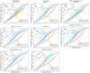 |
Fig. 3. Effects of selecting halos based on their assembly state indicators at z = 0 on their full MAHs. Blue solid lines show the most relaxed third of the halo population at z = 0 according to each parameter, specified in the sub-plot title. Orange dashed lines refer to the most disturbed third. Dark and light contours indicate uncertainty on the mean and population scatter, respectively. The insets indicate the dependence of zform with the corresponding parameter, with a linear fit as the red, dashed line. |
 (10)
(10)
From this, we can obtain zform = z(t = tform). We note that while this definition roughly (but not exactly) agrees with the usual definition of z0.5 as the time where M(z0.5) = M(z0 = 0)/2, it has the advantage of being defined from the whole MAH an hence is less sensitive to oscillations and, especially, to the coarse-graining of the simulation snapshots.
In general, even though the population scatter is large due to the huge diversity of assembly histories, the mean MAHs of the two extreme sub-samples are always clearly separated in the natural direction (i.e. the disturbed sub-sample according to any parameter is more late-forming). However, there are clear variations of the amplitude and the location of such separation amongst the indicators. As a rule of thumb for the following qualitative analysis, we shall indicate the separation to be relevant if the mean of one class falls outside the population scatter of the other.
For some indicators (Δr and  ), the separation of the MAHs is minimal and only focused at very low redshift (a ≳ 0.8), indicating that these parameters are only weakly related with the MAH for under a dynamical time. Wider effects on the MAHs are observed for the rest of indicators.
It is interesting to compare these results to the ones shown in figure 4 of Haggar et al. (2024), where the authors report only noticeable differences in the mean MAHs when stacking them in groups of their PC1 variable (mostly contributed by fsub and Δr), while no significant separation is obtained when using their PC2 (η and concentration; this, however, does encode the spread around the stacked MAH), PC3 (λBullock and cosmic web connectivity), or PC4 (containing ϵ). These findings are slightly at odds with our results (i.e. the fact that most of these parameters do effectively separate the MAHs), which could possibly be due to the fact that their PC variables are linear combinations of many indicators; hence, their influence on the MAH could be lower than the individual variables if they contribute in opposite directions in the linear combination.
However, little further quantitative information can be easily drawn from these panels. This is why we show (in Fig. 4) the Spearman rank-correlation coefficients between M(z)/M0 and each indicator (measured at z = 0) as a function of z. To rule out that any correlation is due to mass dependence on both M(z)/M0 and the assembly state indicator, they are computed as partial correlation coefficients controlling for the dependence on M0 (find a more in-depth description in Sect. 2.5.1). While the figures show the complete information ρM(z)/M0, X|M0 for each indicator X, to simplify the discussion, let us consider that selecting clusters based on X at z0 = 0 is relevant for M(z)/M0 if |ρM(z)/M0, X|M0|> 0.3 at any given z. While this may appear arbitrary8, it does correspond to an identification of the interval of cosmic time where the value of the indicator at z0 = 0 explains over 30% of the scatter on the ranking of the values of M(z)/M0. Here, it is easy to distinguish three groups of indicators:
 |
Fig. 4. Constraining power of the z0 = 0 assembly state indicators on the MAHs. Each panel shows the Spearman rank correlations between the MAH curves and a z0 = 0 assembly state indicator. The absolute magnitude of the curve at each z can be read as the fraction of the scatter on the ranking of M(z)/M0 that can be explained by the corresponding parameter at z0 = 0. The green regions indicate the redshift intervals where this correlation exceeds 0.3 in magnitude, with the green, vertical lines delimiting the interval to ease the visualisation. The horizontal, grey, dashed line marks null correlation. The arrows indicate the redshift at which this correlation is maximal, zc, X. |
-
Late-time indicators, most linked to the MAH at z ≃ 0.1 and no further back than z ≃ 0.2 (≃2τdyn/3 back9): the mean radial velocity (
 ).
). -
Mid-time indicators, being sensitive to M(z)/M0 in the broad redshift interval of 0 ≲ z ≲ 1, with the correlation peaking at z ≃ 0.2 − 0.25 ([0.6 − 0.8]τdyn ago): the virial ratio (η), our combined indicator (χ), and, although at a much less significant level, the centre offset (Δr).
-
Early-time indicators, with their peak correlation with the MAH occurring at z ≃ 0.4 (over a dynamical time ago), and being influenced by the past MAH up to z ≃ 3: sparsity (s200c, 500c), ellipticity (ϵ), sub-structure fraction (fsub), or the spin parameter (λBullock).
It is important noting that a given parameter at z = 0 correlating with the MAH at z ≃ 3 does not equate to the fact that mass accretion at z ≃ 3 is conditioning the value of the parameter at z = 0. This is discussed in greater detail below (Sect. 3.2.2).
Ideally, we could aim to explicitly parametrise the secondary dependence of the MAH on each assembly state indicator M(a|X). However, this is unfeasible in the present study due to the limited statistics, along with the fact that the M(a) values already depend on M0 and that we are considering the whole mass range 1013 M⊙ ≲ Mvir, 0 ≲ 1015 M⊙. Nevertheless, as a first step towards this goal, in the inset of each panel in Fig. 3, we show how zform varies continuously with the corresponding indicator, as obtained from stacking of the MAHs within each decile of the indicator. In this way, even in cases where the separation between the MAHs was not obvious, we find a clear trend for zform (e.g. in the case of Δr; cf. Power et al. 2012, their figure 9).
These dependences can be to first order fitted to linear relations, so as to get the primary trends of formation redshift (and hence, of the MAH; see also Sect. 3.3) with halo properties at z = 0. These results, zform(X), together with their 1σ uncertainties, σzform(X), the validity region of each fit and their R2 values are summarised in Table 1.
3.2.2. What do indicators at a given z tell us about the MARs
While the previous study has focused on characterising the effect on the M(z) curves of selecting clusters and groups based on their assembly state as inferred from different parameters, this is not to be confused by the characteristic epoch of accretion the parameter responds to. That is to say, the fact we have detected significant correlation between, for instance, λBullock and M(z)/M0 back to z ≃ 2.5 is not equivalent to saying that λBullock at z0 = 0 is related to the mass accreted at z = 2.5. This is mostly due to the fact that the MAH curves are strongly self-correlated, in the sense that late-assembling clusters will display stronger slopes at low redshifts and, consequently, lower values at high redshift. To complement this view, in this section we precisely explore the correlations between accretion rates Γ200m (defined in Sect. 2.4) and single assembly state indicators at z = 0 (Fig. 5) and at z = 0.5 (Fig. 6), providing a more insightful picture to assess when each indicator offers specific information.
 |
Fig. 5. Impact of accretion rates on each of the z0 = 0 assembly state indicators. Each panel shows the Spearman rank correlations between the instantaneous MARs and an assembly state indicator at z0 = 0. All plot elements are equivalent to Fig. 4. |
Focusing on the results for the parameters at z = 0 (in line with previous results in Fig. 4), we see that Δr cannot provide sufficient insight on Γ200m (according to our arbitrary threshold of 0.3 on the Spearman rank correlation magnitude). Also, in this case, there is a separation between indicators of earlier and later accretion:
-
In particular, the mean radial velocity
 appears to be the one most focused on present, instantaneous accretion, with
  peaking at z ≃ 0.
 -
Like in the analysis of the MAHs, the virial ratio η and the combined indicator χ are more mid-time indicators of assembly, being sensitive to accretion rates in z ∈ [0, 0.2], peaking around (0.2 − 0.3)τdyn ago.
-
Sub-structure fraction fsub, ellipticity, ϵ, and spin parameter, λBullock, are earlier indicators, being strongly correlated with accretion rates up to z ≃ 0.3 and with their influence being maximal around ∼τdyn/2 from the moment the indicators are determined.
-
Lastly, sparsity stands as the earliest indicator, whose value at z0 = 0 is strongly correlated with the MAR up to z = 0.4 (over a dynamical time ago) and especially at z ≃ 0.2 (∼2τdyn/3 ago)
Among the indicators, the combined parameter χ (Vallés-Pérez et al. 2023, Vallés-Pérez 2024) provides the tightest constraints on the MAR (Spearman correlation magnitude 0.48, implying that this quantity measured at z = 0 can account for half of the scatter in the values of Γ200m at z ≃ 0.07), closely followed by the sub-structure fraction (0.46), although these refer to different epochs as reviewed above.
In an analogous way, in Fig. 6, we analyse which accretion epochs are driving the values of these indicators at z = 0.5. This has the additional interest of being able to assess the correlation between the indicators and, not only past accretion rate, but also future ones. At this earlier time, we can qualitatively discern at least two groups of variables:
 |
Fig. 6. Impact of accretion rates on each of the z = 0.5 (indicated as a vertical, grey, dashed line) assembly state indicators. All plot elements are equivalent to Fig. 5. |
-
Variables responding to the accretion rates in an interval centred on z = 0.5 (the instant when the parameters are determined), namely, the indicators of ongoing accretion. These include the virial ratio (η; roughly in z ∈ [0.45, 0.6]), the mean radial velocity (
 ; z ∈ [0.35, 0.65]) and our combined indicator (χ; for z ∈ [0.4, 0.8]). The latter two display the strongest correlations:
  and ρΓ200m, χ|M0 = 0.48 at their respective peaks.
 -
Variables that are sensitive to past accretion rates, with their correlation peaking around z ≃ 0.65, namely, around ∼0.4τdyn before they are measured. This group consists on halo ellipticity (ϵ; z ∈ [0.55, 0.75]), sub-structure fraction (fsub; z ∈ [0.5, 0.85]), and spin (λBullock; z ∈ [0.55, 0.75]).
Interestingly, even though it does not reach our threshold for significance at this higher redshift, sparsity presents its maximum correlation with the mass increase at z ≃ 0.9, corresponding to a full dynamical time ahead, also in line with the results at z = 0 presented above. This may be naturally explained from the fact that this quantity is sensitive to the density profile in between R200c and R500c. Especially the latter, being a rather central region (R500c ∼ [0.35 − 0.5]R200m), is affected with considerable delay by smooth accretion and mergers (unless these proceed with low impact parameter), whereas the other properties can start to be affected as soon as the infalling matter crosses the outer boundary of the halo.
Although they are indeed subtle, it is important to study these relations at different redshifts through the assembly history of groups and clusters, since, as shown by VP23, the constraining power of these parameters on the presence or absence of assembly episodes varies strongly through cosmic history. While it would be interesting to pursue these analyses at higher redshift, in the present work we are limited by several factors, including the sparse saving of snapshots (ideally, we need around 6 − 10 snapshots per dynamical time to be able to appreciate timing differences across indicators), or the increasing uncertainty of the determination of merger tree’s main branches (which becomes less straightforward as we approach the protocluster regime beyond z ∼ 1.5 − 2).
3.3. Constraints on the MAHs from individual indicators at z = 0
Given the complexity and diversity of MAHs, we deal in Sect. 3.3.1 with the possibility of summarising this diversity with two parameters. Subsequently, in Sect. 3.3.2, we study how our assembly state indicators provide constraints in this biparametric space.
All the results in this section correspond exclusively to the sub-sample of clusters that can be tracked back to zstart = 4. Such a selection may induce a slight bias for the MAHs, as it has been shown that major mergers pose an important challenge for halo finders and merger trees, particularly in recovering halo masses (Behroozi et al. 2015). Nevertheless, we have explicitly verified that the discrepancy, at high redshift, between the MAH stacked over the whole cluster sample, and only those tracked back to z > zstart, does not exceed ∼30%. Given that MAHs typically span over two orders of magnitude in our sample (see Fig. 1), this level of discrepancy is minor, and the approach remains robust.
3.3.1. Biparametric characterisation of the MAHs
To reduce the dimensionality of the problem, we aim to capture as much information as possible from the MAHs (a continuous function) with a minimal set of parameters. This was done, from the data-driven perspective, by Wong & Taylor (2012), for instance. They performed a principal component analysis (PCA; Pearson 1901; Hotelling 1936) on their assembly histories to extract and interpret the two most relevant contributions. Here, conversely, we have aimed to define two properties of the MAH with closed mathematical forms to explore the extent to which they capture the diversity of MAHs.
The first of such properties is, naturally, the formation redshift, zform, as defined by Eq. (10). This quantity (or alternative definitions, such as z0.5) has been widely used in the literature. As a second parameter aimed at explaining the scatter in assembly histories at fixed formation time, we introduced a dimensionless quantity, αMAH, measuring the episodicity of the assembly (i.e. whether it occurs suddenly in one major event, or more smoothly throughout the whole evolutionary history). Formally, we define it as
 (11)
(11)
where tβ is the latest time when M(tβ) = βM0 (0 < β ≤ 1). In this way, high values of αMAH indicate smooth assembly, and low values indicate bursty assembly around the formation time of the halo10.
In the two upper panels of Fig. 7, we plot all MAHs, normalised as M200m(a)/M200m(a0 = 1), colour-coded by zform (left-hand side panel) and by αMAH (right-hand side panel). The interpretation of the former is direct, earlier-assembling clusters having larger – yellow – values of zform (in contrast, later-assembling clusters having smaller – purple – values). Clusters with large αMAH (yellow lines) have straighter MAHs, indicative of a smoother – at a more constant pace – assembly of their mass. Conversely, the smaller the value of αMAH (turquoise to purple lines), the larger the variation in the steepness of these curves, presenting a very steep build-up of mass around zform (coming from one or several successive major mergers) and a quiescent phase for the rest of their assembly history.
 |
Fig. 7. Parametrisation of the MAHs. The two top panels present the assembly histories of the whole sample, colour-coded according to the formation redshift zform (left) and the episodicity parameter αMAH (right-hand side panel). The two bottom panels describe the distribution of these parameters in the {PC1, PC2} space, accounting for the maximum variance with two linearly uncorrelated components. The colour coding of the dots is the same as represented in their respective top panels. |
While this parametrisation is fully physically motivated, it is still imperative to check to what extent does it describe the diversity of assembly histories. To this end, we performed a PCA on our MAHs, qualitatively reproducing the results by Wong & Taylor (2012) for the two first components, jointly accounting for 77% of their total variance (cf. 83% in the aforementioned reference; for a thorough description, see Appendix B).
In the two lower panels of Fig. 7, we plot the distribution of our assembly histories in the {PC1, PC2} space, colour-coded according to zform (left) and αMAH (right) following the colour bars in the respective panels above. There is a very clean correlation (albeit non-linear) between zform and PC1, resulting in a Spearman rank correlation ρsp(zform, PC1) = − 0.975, justifying our choice in Sect. 3.2 to characterise the dependence of zform on our indicators, as the main summary statistic of the full MAH.
For αMAH, from the bottom right panel of Fig. 7 it is obvious that, at fixed PC1, PC2 is significantly anticorrelated with αMAH. To quantify the strength of such a correlation, since data points in the {PC1, PC2} are distributed in an arc-like shape (i.e. non-monotonic), we used the non-parametric residual correlation introduced in Sect. 2.5.1. In this way, we were able to obtain that the residuals with respect to the underlying PC2 = f(PC1) relation have a Spearman rank correlation of −0.68 with αMAH (up to −0.72 if discarding the most extreme outliers, |PC1|> 10). This implies that our set of two physically motivated variables describe, to a considerably large extent, the main variability of the assembly histories in our sample as revealed by the PCA, and therefore are in principle a good choice to study the dependence of the MAHs on assembly state indicators at z = 0 below.
3.3.2. Constraints on the MAHs from the assembly state indicators
Having defined a 2D space where the complexity of MAHs can be summarised, we can now investigate what direction in this space is constrained by each of the indicators in Sect. 2.3. We do so under the assumption of monotonous, but not necessarily linear, dependences of our parameters with the MAHs within this space, which is well justified based on the findings of the previous Sect. 3.2.
Following the procedure of Sect. 2.5.2, for each of the parameters, X, at z = 0 we can obtain a vector ρ(X) representing the direction in which X varies, and the magnitude of such dependence (the larger it is, the more information about the MAH that the parameter can yield). This is represented, both in the zform − αMAH and in the PC1 − PC2 planes, in the upper and lower panels of Fig. 8, respectively.
 |
Fig. 8. Constraints of the assembly state indicators on the two biparametric characterisations of the MAHs: the zform − αMAH plane (top panel) and the PC1 − PC2 plane (bottom panel). In each panel, the different arrows correspond to each of the assembly indicators according to the colour legend in the bottom panel. Their directions indicate the relative weight of each of the two parameters in the linear combination which best correlates with the given indicator, while their magnitude is the Spearman rank correlation coefficient between the indicator and the corresponding projection of the MAH representation (the larger, the more information is yielded by the indicator). Colour aid: Arrows correspond to χ, Δr, fsub, λBullock, |


In the former case, namely, in the zform − αMAH plane, it appears that little information can be obtained on the episodicity of accretion from this set of parameters (vectors are mostly horizontal). Only Δr provides very marginal (p-value = 0.11) correlation with αMAH, while the only relevant information being drawn from the remaining of parameters lies in the early-late assembly axis, (i.e. corresponding to zform). Naturally, our combined indicator χ points in the opposite direction to the individual ones, since it measures relaxedness, as opposed to the rest which are intuitively measures of disturbance. Strikingly, amongst these parameters, it is the spin parameter the one most correlated with the MAH (mainly, zform), achieving a Spearman rank correlation of 0.68.
Perhaps more interestingly, if we look at these relations in the PC1 − PC2 plane, there is a broader separation of these vectors, indicating that one can obtain broader information on these parameters from the assembly state indicators. In particular, general trends are maintained (e.g. the spin parameter yielding the most amount of information, χ indicating relaxedness and hence being opposed to the other indicators, etc.). However, there is a greater scope of the range of information about the MAH yielded by each parameter. For instance, while halo spin informs provides information exclusively about the formation time (larger spin implying later assembly), a larger centre offset is indicative of smoother accretion (less episodic) regardless of formation time. Other indicators (sub-structure fraction, sparsity, ellipticity, virial ratio, and mean radial velocity) lie in between these extreme cases, encompassing increasingly more information about PC2 in the order specified above.
Despite the low significance of the results in the zform − αMAH plane, it might be striking how Δr appears as an indicator of ‘bursty’ accretion when assessed in the zform − αMAH space, while it indicates smoother accretion in the principal components space. These results are not necessarily at odds with each other, but rather reflect that PC2 and αMAH (contrary to PC1 and zform) are correlated but not fully co-dependent. Thus, even though we have dubbed both the regimes of high PC2 and low αMAH as bursty accretion, they represent episodicity in different senses. While αMAH represents a mean accretion rate in a long and variable time interval (between the instant when 25% and 75% of the present-day mass was built up), PC2 is focused at a particular redshift (around a ≃ 0.65; see Fig. B.1). Additionally, despite the fact that αMAH appears to be more physically motivated, it is reasonable that we see more significant relations with PC2, since (by construction) the latter variable captures more variance of the MAHs than the former.
 |
Fig. 9. Assembly histories for individual clusters (summarised in the PC1 − PC2 plane) colour-coded according to each of the assembly state indicators at z = 0. The colour bars are ordinal (i.e. linear in the ranked variable: e.g. the middle point of the colorbar corresponds to the median value). At the top of each panel, we indicate the direction of maximum correlation with the indicator, the Spearman rank correlation coefficient, and the Kendall rank correlation coefficient. |
This is why we focus on the PC1 − PC2 space (as shown in Fig. 9) to represent the diversity of assembly histories in our sample of halos, colour-coded according to each of the indicators. Generally, trends are difficult to identify visually due to the considerable scatter. This is why, in the top part of each panel, we have annotated the direction of maximum correlation with the variable represented in colour, the magnitude of such correlation, and also the Kendall rank correlation coefficient (see Sect. 2.5.3 for the definitions). Thus, the arrows and Spearman coefficients present identical information to what has been shown in the lower panel of Fig. 8, but the scatter plot and τK values give a clearer view on how much information is brought by each single parameter.
In particular, a probabilistic interpretation of τK(x, y) comes by noting that the probability that, if x1 ≥ x2, then y1 ≥ y2, is precisely (1 + τK)/2. Therefore, the most promising indicator for constraining the past formation history of galaxy clusters and groups is, consistent with previous results, λBullock. In this case, finding a cluster with higher spin parameter than another one gives 75% probability that it will be later forming (more precisely, it will have a larger component along the direction specified by the arrow in the bottom, left panel of Fig. 9, which is essentially the zform axis).
Other parameters (fsub, s200c, 500c, etc.) still provide significant constraints on the position of the cluster in this assembly history representation space, while in other cases (Δr,  ) the information on a cluster-to-cluster basis is marginal (τK ≲ 0.2, implying probabilities of concordant pairs below 60%, which is only marginally better than random guessing).
Therefore, in an ensemble sense, these parameters predict a very noticeable segregation of the MAH curves and derived parameters (see Sect. 3.2), which could be useful, for instance, for sample selection. However, on a one-to-one basis, the population scatter is sufficiently large to significantly worsen the prospects of determining the assembly history of a halo by looking at a single parameter. Nevertheless, as we have shown, different parameters provide constraints in different directions in this space that summarises the MAHs. Hence, this leaves the door open for the combination of different indicators to better constrain the location of objects in this space.
3.4. Assembly state inferred from the ICM distribution
All the quantities involved in the study are derived from the dark matter distribution. As a first step towards the connection of these quantities to actually observable data, in this section we explore how much of this information is contained in the ICM morphology and dynamics. While the ICM properties defined here are not directly observable, a tight correlation between 3D ICM and DM properties is a necessary (but not sufficient) condition for SZ and X-ray morphology to be capable of constraining assembly state. In Sect. 3.4.1 we describe how we compute these parameters for the gas distribution, while the results of the comparison are discussed in Sect. 3.4.2.
3.4.1. Definition of the indicators for the ICM
In order to define an equivalent set of indicators computed from the ICM (again using the whole, 3D description), we need to modify the definition or the computation process of several of the parameters. In particular,
-
Centre offset. The computation of the centre of mass is analogous to the DM case. For the gas density peak, however, instead of following the procedure described in Vallés-Pérez et al. (2022) for DM particles, we take advantage of the AMR grid. Thus, we iterate from coarser to finer levels in the AMR hierarchy, each time finding the density peak in a 3 × 3 × 3-cells neighbourhood of the location determined at the previous AMR level. This iteration is especially important in our case, since the usage of simulations with cooling but no feedback can produce a significant number of unphysical clumps away from the cluster centre.
-
Virial ratio. Due to the collisional nature of gas, most of its kinetic energy (T) is converted into internal (Uth). Thus, we consider the quantity T′=(T + Uth)/fB, where fB = 0.155 is the cosmic baryon fraction, under the assumption that the total kinetic energy can be extrapolated to the whole mass distribution. Similarly, from the gravitational binding energy of the gas to itself (Ugas), we estimate U′=Ugas/fgas2.
-
Sparsity. In this case, sparsity is computed as by finding MΔc, gas as the mass within a sphere containing a mean gas overdensity, Δgas = fgasΔc, with respect to the critical ΛCDM density.
-
Sub-structure fraction. The notion of sub-structure is fundamentally different for the ICM and for the DM halo. Many DM sub-structures do not have a corresponding gaseous halo, while the ICM contains many clumps not associated with a DM sub-structure. This is why we have opted to quantify gaseous sub-structure in its most natural way, using a method based on Zhuravleva et al. (2013). Essentially, we took directional profiles of the ICM density with Δlog r = 0.01 dex and, at each r, we flagged all volume elements exceeding a density
 as a gaseous sub-structure (i.e. clumps). Here,
  is the median density, σlog ρ is the standard deviation of log ρ and fcut = 3.5 is a free parameter, for which we used the same prescription as in Zhuravleva et al. (2013).
The rest of indicators not mentioned here were computed in the same way as for DM. As for our combined indicator χ, since it corresponds to an empirical calibration of thresholds and weights, it lacks sense applying it directly to other indicators defined from the gas distribution. We note that the dynamics of the ICM is strongly affected by galaxy formation physics and other physical effects (e.g., viscosity) not considered in this simulation. Thus, one can expect shifts in the values of these indicators (e.g. feedback may suppress clumping, thus reducing sub-structure fraction from gas). The simpler physical setup in this simulation lets us isolate the effects of structure formation driven phenomena.
3.4.2. Assembly state indicators from the ICM
The results of the comparison between the set of indicators computed from the DM distribution and from the ICM distribution, are summarised in Fig. 10. In general, there are positive correlations for most of the parameters, but the scatter is sufficiently high to prevent a clear measurement of DM halo properties from ICM properties.
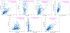 |
Fig. 10. Correspondence between the assembly state indicators measured from the DM distribution (horizontal axes) and from the ICM distribution (vertical axes), at z = 0. Each panel corresponds to a different parameter. Within each panel, each dot corresponds to a cluster or group; the dashed, gray line is the identity relation (Xgas = XDM); and the dashed red line is a least-squares linear fit, whose slope (m) is given at the top of each panel. Also the Spearman and Kendall rank correlation magnitudes, and their p-values, are given there. |
In many cases (Δr,  , ε, and λBullock), DM and gas indicators show a moderate (ρs ∼ 0.3 − 0.6) correlation, with very significant scatter, and a slope m < 1 (represented with the dashed, red line), clearly inconsistent with a direct one-to-one relation (represented by the dashed, gray line). This is most likely associated to the collisional nature of the ICM, which tends to produce rounder shapes (Lau et al. 2011, 2012), with consequently lower Δr, and lower infall velocities.
For these indicators (with the exception of λBullock), there are strong outliers above the fitted relation, indicating the presence of objects with very disturbed gas morphology, compared to their DM distribution. It is plausible that the presence of unopposed cooling in this simulation is generating some of these very disturbed morphologies, although fully elucidating their origin falls beyond the scope of the present work.
Amongst all these parameters, λBullock is shown to yield the relation with the least scatter. This is interesting, since this quantity also presents the largest correlations with assembly history (see Sect. 3.3). Additionally, this quantity could, potentially – and only in projection–, be determined by kinetic Sunyaev-Zeldovich measurements (Baldi et al. 2018; albeit with large scatter, cf. Monllor-Berbegal et al. 2024), rendering it a useful indicator to further study in both theoretical and observational data.
Other cases present even more striking differences between gas and DM. In particular, η values are essentially uncorrelated amongst the two components, signalling that the naive corrections by fgas suggested in Sect. 3.4.1 are not effective. To some degree, this could be contributed by the departure of fgas from its cosmic average (used for the corrections on T′ and U′). However, this simulation lacks feedback and fgas values present a rather narrow distribution, only slightly below the cosmic value. Instead, the most likely explanation for the lack of correlation resides in the different density profiles of both components, which make the comparison between gravitational energies inferred from the gas or from the total mass not straightforward. Perhaps less surprising is the lack of correlation between sub-structure fractions. Generally, we find cases of, both, rich DM sub-structure with no gaseous sub-structure and, more abundantly, the opposite. This is reasonable since these sub-structures have fundamentally different origins: the DM one comes from accretion of smaller halos, while the gaseous one (clumpiness) occurs in-situ due to cooling, even though it has also been linked to different measures of dynamical unrelaxedness (Roncarelli et al. 2013; Vazza et al. 2013; Battaglia et al. 2015; Planelles et al. 2017).
Lastly, the case of sparsity is interesting, since it presents a moderate correlation with slope m > 1. That is to say, while clusters appear more relaxed in their gaseous component when using indicators such as Δr or ε, the opposite trend is seen for s200c, 500c. As a matter of fact, gas sparsity appears to be approximately lower-bounded by DM sparsity, as a result of the gas distribution usually being less concentrated.
In summary, while in some cases DM and gas indicators present moderate correlations, the determination of these indicators from ICM data appears to be complex and affected by high scatter (let aside projection effects). Furthermore, these correlations are not scattered around the identity – and, rather, the slope might be larger or smaller than unity – so care must be taken when comparing relaxation criteria amongst different components.
4. Discussion and conclusions
In this work, we have used a moderate-sized hydrodynamical + N-Body cosmological simulation to study the connection between DM halo and ICM properties and the full assembly history of a sample of galaxy clusters and groups (1013 M⊙ ≤ Mvir ≲ 8 × 10¹⁴ M⊙) through the redshift interval 4 ≥ z ≥ 0. The extreme diversity in the formation channels of these structures demands a careful study of how these complex processes shape their properties, the timescales on which they are imprinted, and what the extent is of such an effect. The main findings of this paper can be summarised and put into context within the bibliography as follows.
Results summary for the timing analysis (central block) and the biparametric analysis (right-hand side block) on the MAHs, with each indicator given in each row.
-
The strategy for building the merger tree and, especially, selecting its main branch, is critical for determining and comparing the MAHs. In particular, at z ≃ 4, ours (where the main branch of the merger tree is determined on the basis of gravitational binding) are shown to reside a factor of ∼3 [∼2] below those of Correa et al. (2015) (van den Bosch et al. 2014), both of which are based on selecting the most massive progenitor. While there is no ‘true’ solution for defining the main branch of the merger tree, it is important to take caution when comparing amongst works in the literature, since different choices lead to noticeable differences. In particular, in Appendix A we show how – if we switch our strategy for defining the main branch – our MAHs are brought to substantially better agreement with the previously mentioned works.
-
As already discussed in different forms by Jeeson-Daniel et al. (2011), Skibba & Macciò (2011), and Haggar et al. (2024), indicators for the dynamical state of a cosmic structure (either galaxy clusters or their DM halos) are rather loosely correlated. In Fig. 2 we have shown how only a few pairs of parameters reach Spearman correlation ranks above ρs ∼ 0.4. This already suggests that (i) the information brought on by a single indicator can be fairly limited in a cluster-by-cluster basis and (ii) combinations of parameters might be useful to improve the predictive power on the MAHs, as done for instance by VP23.
-
Selecting clusters based on the assembly state indicators defined in Sect. 2.3 clearly splits their ensemble (stacked) MAHs in such a way that (according to any given parameter at z = 0) the higher the value of these indicators, the more late-forming the object is (Fig. 3).
-
Upon closer inspection (Fig. 4), these quantities are especially informative about different moments of the MAHs, enabling us to categorise them into more late-time (e.g.
 , η) and more early-time (e.g. ϵ, λBullock) indicators.
 -
We have calibrated relations for the formation redshift, zform, as a function of our different indicators (Table 1). With the exception of
 , these relations are tight and could be useful to understand the effects of selecting clusters based on their properties. Additionally, they could also help inform (semi-)analytic models (e.g. halo occupation distribution or similar methods).
-
-
Looking at the correlations between instantaneous accretion rates and indicators, we obtained a clearer view on the timescale each indicator is relevant to. Our results show how the indicators contain information about the accretion rates in different moments of the halo history. These range from instantaneous indicators (
 ) to late-time accretion indicators (η and χ, sensitive to z ∈ [0, 0.2] accretion rates), early-time accretion rate proxies (fsub, ϵ, λBullock, around z ≃ 0.3), and, finally, s200c, 500c provides the earliest information and demonstrates the ability to partially constrain the accretion rate up to z ≃ 0.4 when measured at z = 0. A more detailed summary is presented in Table 2.
 -
We have studied the characterisation of the diversity of MAHs with a couple of parameters (zform and αMAH) that can be defined with closed analytical forms from the M(a) curves. These parameters can be understood as having a steady correspondence (albeit a non-linear one) to the two principal components of the MAHs, as extracted from the PCA algorithm reproducing the analysis of Wong & Taylor (2012).
-
We characterised the information brought by each assembly state indicator on both biparametric representations of the MAHs. While, in the zform − αMAH space, the indicators are essentially incapable of constraining the episodicity parameter, αMAH. However, they can indeed offer a richer store of information in the PC1 − PC2 space. In this space, some indicators can be more informative about the formation time (e.g. λBullock), and others mainly offer insights into how episodic or bursty the accretion history has been, while being essentially unrelated to the assembly time (e.g. Δr). Most parameters (including our combined indicator, χ) lie in the middle ground, thus providing a combination of information on these two evolutionary properties. This information is summarised in an indicator-by-indicator basis in Table 2.
-
Regardless of the trends obtained in this work, it is important to note how (while here we have mostly concentrated on the effect of the assembly state indicators on the ensemble properties of halos) assessing the formation history of an individual galaxy cluster or group based on single properties is very difficult. This is the case due to the high intrinsic (cluster-to-cluster) scatter in the relations (e.g. 1σ uncertainties of Δzform ∼ 0.2 in Table 1; see also e.g. figure 8 of Wong & Taylor 2012). This is, at least in part, due to the non-trivial evolution of these indicators. While all of them tend to increase with recent strong assembly activity, their particular evolution during smooth accretion episodes and mergers might not necessarily be trivial. For instance,
 is by definition insensitive to mergers during their pericentric passages, as are Δr and ϵ (to a lesser extent). Due to the intrinsic interest of this topic, we plan to address the relation of these quantities to mergers in a future, separate work.
 -
In the case where the same indicators primarily used in this work (derived from the DM distribution) are derived (with minimal adaptations) from the ICM gaseous distribution, once again, the high scatter makes it essentially impossible to relate the DM morphological and dynamical parameters to gas properties (or vice versa) on a cluster-to-cluster basis; noting, however, that there are moderate correlations. For example, in the best case, measuring a larger spin parameter, λBullock, from the gas distribution only implies a larger rotation of DM in ∼75% of the cases. This suggests that assessing the dynamical state of a cluster in observations from single (ICM) morphological parameters may not be an accurate method – or, rather, the conclusions may not be directly extrapolated from the ICM to DM. This could only possibly be overcome by the (likely non-linear) combination of many different indicators, which might additionally be redshift- and mass-dependent, as hinted by VP23.
The results presented in this work contribute to the existing bibliographic corpus in suggesting that dynamical state is not a single, monolithic property (e.g. Haggar et al. 2024), and they do complement previous approaches in similar directions (e.g. Wong & Taylor 2012) by incorporating baryons (which are known to modify several of the parameters involved in this study) and looking at the constraining power of these parameters on the actual accretion rates, as well as the timing of the accretion phenomenology.
Overall, we have shown how: (i) the stacked MAHs are strongly dependent, even up to z ≃ 4, on selection of the clusters and groups based on the value of their indicators at z = 0; (ii) the different indicators respond to mass accretion in distinct moments through the assembly history (from instantaneous, to a τdyn ago; and (iii) each indicator points in different directions in the parameter space summarising the MAHs, implying that they may be able to constrain, not only the formation time, but also secondary properties (e.g. how smooth or bursty this accretion is).
Future works will need to deal with how the information obtained from the full 3D description offered by simulations (as in the present work) is retained or hindered when obtained from observations. When dealing with observations, it will also be interesting to see in how far these theoretical measures of cluster assembly can be related to, for instance, X-ray and SZ morphology (e.g. Zenteno et al. 2020; Capalbo et al. 2021), or the properties of the galaxy populations (Berrier et al. 2009). Conceptually, this involves several steps that should be carefully considered: the relation between DM halo and ICM properties and galaxy distribution under varying physical models (including feedback prescriptions), the effects of projection, and the observational constraints of present and future instruments. In forthcoming works of this series, we will concentrate on the effect of cluster assembly on the dynamical and thermodynamical properties of the ICM.
Here, Mvir is the virial mass using the prescription of Bryan & Norman (1998), which corresponds to the mass in a spherical overdensity Δc = 18π2 + 39[Ωm(z)−1] − 82[Ωm(z)−1]2 with respect to the critical density ρc = 3H2/(8πG), G being the gravitational constant. At z = 0, this corresponds to Δm, vir ≊ 330.7.
We adopt the usual notation for MΔc[m] being the mass in a sphere of radius RΔc[m] enclosing an overdensity Δ times the critical [background] density of a ΛCDM cosmology.
We opted for R200m as the aperture to define our MAHs, instead of the Rvir described in Sect. 2.2 to define the cluster sample, since the latter would introduce an explicit pseudoevolution of the MAHs due to the time-dependent overdensity.
Note that the Spearman rank correlation coefficients are just the Pearson coefficients between the rank variables. Hence, instead of testing for linearity, they indicate monotonicity.
We note that this weak correlation of η with M200m vanishes if we account for the surface energy term in the computation of the virial ratio, as in Shaw et al. (2006). Nevertheless, the corrected ratio, η′, does not correlate with assembly state, as discussed above and in Vallés-Pérez et al. (2023).
The results on the timing of the different indicators are by construction unchanged by this threshold (i.e. the curves and the green arrow in Fig. 4). The choice of explaining 30% of the scatter to be deemed as relevant is, by definition, arbitrary, and whether it is enough or not will inevitably depend on the application.
τdyn(z) = [Gρ]−1/2 = [GρB(z)Δvir(z)]−1/2 is the dynamical timescale associated to the virial density of a collapsed DM halo, where ρB(z) = Ωm(z)ρc(z) is the background matter density and Δvir(z) is the virial overdensity given by Bryan & Norman (1998).
We have tested either normalising t0.75 − t0.25 by τdyn(zform) and by τdyn(z = 0), finding that in the latter case there is a small but significant (ρsp ∼ −0.3) anticorrelation of the resulting parameter with zform. Hence, the former appears to be a more convenient choice to represent the MAHs. It is also worth to mention that, while for zform we chose not to use quantile-based measurements (z0.5), this is not as problematic for αMAH since the noisy character associated to the coarse-graining of the snapshots is heavily suppressed by the fact that t0.75 − t0.25 typically corresponds to 5 − 10 snapshots.
At a0 = 1, we naturally encounter a node since ℳj(a0 = 1) = 1 for all j by construction. At the high-redshift end, however, we find an approximate node: while here not all values of ℳj(a ≈ 0.2) are equal, they typically lie in the interval [0.01, 0.1], thus much smaller than 1.
Acknowledgments
We thank the anonymous referee for their valuable feedback, which has contributed to improve the presentation of this work. This work has been supported by the Agencia Estatal de Investigación Española (AEI; grant PID2022-138855NB-C33), by the Ministerio de Ciencia e Innovación (MCIN) within the Plan de Recuperación, Transformación y Resiliencia del Gobierno de España through the project ASFAE/2022/001, with funding from European Union NextGenerationEU (PRTR-C17.I1), and by the Generalitat Valenciana (grant CIPROM/2022/49). DVP acknowledges support from Universitat de València through an Atracció de Talent fellowship. The simulation and part of the analysis has been carried out using the supercomputer Lluís Vives at the Servei d’Informótica of the Universitat de València. This research has been made possible by the following open-source projects: Numpy (Harris et al. 2020), Scipy (Virtanen et al. 2020), Matplotlib (Hunter 2007), FFTW (Frigo & Johnson 2005), emcee (Foreman-Mackey et al. 2013).
References
- Angelinelli, M., Vazza, F., Giocoli, C., et al. 2020, MNRAS, 495, 864 [NASA ADS] [CrossRef] [Google Scholar]
- Angelinelli, M., Ettori, S., Vazza, F., & Jones, T. W. 2021, A&A, 653, A171 [NASA ADS] [CrossRef] [EDP Sciences] [Google Scholar]
- Baker, W. M., Maiolino, R., Bluck, A. F. L., et al. 2022, MNRAS, 510, 3622 [NASA ADS] [CrossRef] [Google Scholar]
- Baldi, A. S., De Petris, M., Sembolini, F., et al. 2018, MNRAS, 479, 4028 [NASA ADS] [CrossRef] [Google Scholar]
- Balmès, I., Rasera, Y., Corasaniti, P. S., & Alimi, J. M. 2014, MNRAS, 437, 2328 [CrossRef] [Google Scholar]
- Battaglia, N., Bond, J. R., Pfrommer, C., & Sievers, J. L. 2015, ApJ, 806, 43 [NASA ADS] [CrossRef] [Google Scholar]
- Beers, T. C., Flynn, K., & Gebhardt, K. 1990, AJ, 100, 32 [Google Scholar]
- Behroozi, P., Knebe, A., Pearce, F. R., et al. 2015, MNRAS, 454, 3020 [Google Scholar]
- Bennett, J. S., & Sijacki, D. 2022, MNRAS, 514, 313 [CrossRef] [Google Scholar]
- Berrier, J. C., Stewart, K. R., Bullock, J. S., et al. 2009, ApJ, 690, 1292 [NASA ADS] [CrossRef] [Google Scholar]
- Biava, N., Bonafede, A., Gastaldello, F., et al. 2024, A&A, 686, A82 [NASA ADS] [CrossRef] [EDP Sciences] [Google Scholar]
- Binney, J., & Tremaine, S. 1987, Galactic Dynamics (Princeton, N.J.: Princeton University Press) [Google Scholar]
- Bond, J. R., Kofman, L., & Pogosyan, D. 1996, Nature, 380, 603 [NASA ADS] [CrossRef] [Google Scholar]
- Bryan, G. L., & Norman, M. L. 1998, ApJ, 495, 80 [NASA ADS] [CrossRef] [Google Scholar]
- Bullock, J. S., Kolatt, T. S., Sigad, Y., et al. 2001, MNRAS, 321, 559 [Google Scholar]
- Campitiello, M. G., Ettori, S., Lovisari, L., et al. 2022, A&A, 665, A117 [NASA ADS] [CrossRef] [EDP Sciences] [Google Scholar]
- Capalbo, V., De Petris, M., De Luca, F., et al. 2021, MNRAS, 503, 6155 [Google Scholar]
- Cataldi, P., Pedrosa, S. E., Tissera, P. B., et al. 2023, MNRAS, 523, 1919 [NASA ADS] [CrossRef] [Google Scholar]
- Chen, H., Avestruz, C., Kravtsov, A. V., Lau, E. T., & Nagai, D. 2019, MNRAS, 490, 2380 [NASA ADS] [CrossRef] [Google Scholar]
- Cole, S., & Lacey, C. 1996, MNRAS, 281, 716 [NASA ADS] [CrossRef] [Google Scholar]
- Corasaniti, P. S., Ettori, S., Rasera, Y., et al. 2018, ApJ, 862, 40 [CrossRef] [Google Scholar]
- Corasaniti, P. S., Richardson, T. R. G., Ettori, S., et al. 2025, A&A, 697, A33 [NASA ADS] [CrossRef] [EDP Sciences] [Google Scholar]
- Correa, C. A., Wyithe, J. S. B., Schaye, J., & Duffy, A. R. 2015, MNRAS, 450, 1514 [NASA ADS] [CrossRef] [Google Scholar]
- Cramer, H. 1946, Mathematical Methods of Statistics (Princeton Univ. Press) [Google Scholar]
- Crone, M. M., Evrard, A. E., & Richstone, D. O. 1996, ApJ, 467, 489 [Google Scholar]
- Cui, W., Power, C., Biffi, V., et al. 2016, MNRAS, 456, 2566 [NASA ADS] [CrossRef] [Google Scholar]
- Cui, W., Power, C., Borgani, S., et al. 2017, MNRAS, 464, 2502 [NASA ADS] [CrossRef] [Google Scholar]
- De Boni, C., Serra, A. L., Diaferio, A., Giocoli, C., & Baldi, M. 2016, ApJ, 818, 188 [NASA ADS] [CrossRef] [Google Scholar]
- Diemer, B., Mansfield, P., Kravtsov, A. V., & More, S. 2017, ApJ, 843, 140 [NASA ADS] [CrossRef] [Google Scholar]
- Dierckx, P. 1995, Curve and Surface Fitting with Splines (Clarendon Press), Monogr. Numer. Anal. [Google Scholar]
- Dolag, K., Vazza, F., Brunetti, G., & Tormen, G. 2005, MNRAS, 364, 753 [NASA ADS] [CrossRef] [Google Scholar]
- Duffy, A. R., Schaye, J., Kay, S. T., et al. 2010, MNRAS, 405, 2161 [NASA ADS] [Google Scholar]
- Eckert, D., Roncarelli, M., Ettori, S., et al. 2015, MNRAS, 447, 2198 [Google Scholar]
- Eisenstein, D. J., & Hu, W. 1998, ApJ, 496, 605 [Google Scholar]
- Foreman-Mackey, D., Hogg, D. W., Lang, D., & Goodman, J. 2013, PASP, 125, 306 [Google Scholar]
- Frigo, M., & Johnson, S. G. 2005, Proc. IEEE, 93, 216, special issue on “Program Generation, Optimization, and Platform Adaptation” [Google Scholar]
- Giocoli, C., Tormen, G., & Sheth, R. K. 2012, MNRAS, 422, 185 [NASA ADS] [CrossRef] [Google Scholar]
- Gott, J. R., I., & Rees, M. J. 1975, A&A, 45, 365 [NASA ADS] [Google Scholar]
- Gouin, C., Bonnaire, T., & Aghanim, N. 2021, A&A, 651, A56 [NASA ADS] [CrossRef] [EDP Sciences] [Google Scholar]
- Haggar, R., Gray, M. E., Pearce, F. R., et al. 2020, MNRAS, 492, 6074 [NASA ADS] [CrossRef] [Google Scholar]
- Haggar, R., De Luca, F., De Petris, M., et al. 2024, MNRAS, 532, 1031 [Google Scholar]
- Harris, C. R., Millman, K. J., van der Walt, S. J., et al. 2020, Nature, 585, 357 [NASA ADS] [CrossRef] [Google Scholar]
- Hotelling, H. 1936, Biometrika, 28, 321 [Google Scholar]
- Hunter, J. D. 2007, Comput. Sci. Eng., 9, 90 [NASA ADS] [CrossRef] [Google Scholar]
- Jeeson-Daniel, A., Dalla Vecchia, C., Haas, M. R., & Schaye, J. 2011, MNRAS, 415, L69 [NASA ADS] [Google Scholar]
- Kendall, M. G. 1938, Biometrika, 30, 81 [Google Scholar]
- Kimmig, L. C., Remus, R.-S., Dolag, K., & Biffi, V. 2023, ApJ, 949, 92 [Google Scholar]
- Kimmig, L. C., Brough, S., Dolag, K., et al. 2025, A&A, submitted [arXiv:2503.20857] [Google Scholar]
- Knebe, A., & Power, C. 2008, ApJ, 678, 621 [NASA ADS] [CrossRef] [Google Scholar]
- Knebe, A., Knollmann, S. R., Muldrew, S. I., et al. 2011, MNRAS, 415, 2293 [Google Scholar]
- Kravtsov, A. V., & Borgani, S. 2012, ARA&A, 50, 353 [Google Scholar]
- Lau, E. T., Kravtsov, A. V., & Nagai, D. 2009, ApJ, 705, 1129 [NASA ADS] [CrossRef] [Google Scholar]
- Lau, E. T., Nagai, D., Kravtsov, A. V., & Zentner, A. R. 2011, ApJ, 734, 93 [CrossRef] [Google Scholar]
- Lau, E. T., Nagai, D., Kravtsov, A. V., Vikhlinin, A., & Zentner, A. R. 2012, ApJ, 755, 116 [NASA ADS] [CrossRef] [Google Scholar]
- Lau, E. T., Nagai, D., & Nelson, K. 2013, ApJ, 777, 151 [NASA ADS] [CrossRef] [Google Scholar]
- Lau, E. T., Nagai, D., Avestruz, C., Nelson, K., & Vikhlinin, A. 2015, ApJ, 806, 68 [NASA ADS] [CrossRef] [Google Scholar]
- Lau, E. T., Hearin, A. P., Nagai, D., & Cappelluti, N. 2021, MNRAS, 500, 1029 [Google Scholar]
- Lourenço, A. C. C., Jaffé, Y. L., Vulcani, B., et al. 2023, MNRAS, 526, 4831 [CrossRef] [Google Scholar]
- Lovisari, L., Forman, W. R., Jones, C., et al. 2017, ApJ, 846, 51 [Google Scholar]
- Macciò, A. V., Dutton, A. A., van den Bosch, F. C., et al. 2007, MNRAS, 378, 55 [Google Scholar]
- Maulbetsch, C., Avila-Reese, V., Colín, P., et al. 2007, ApJ, 654, 53 [NASA ADS] [CrossRef] [Google Scholar]
- McBride, J., Fakhouri, O., & Ma, C.-P. 2009, MNRAS, 398, 1858 [NASA ADS] [CrossRef] [Google Scholar]
- McCarthy, I. G., Babul, A., Bower, R. G., & Balogh, M. L. 2008, MNRAS, 386, 1309 [NASA ADS] [CrossRef] [Google Scholar]
- Monllor-Berbegal, Ó., Vallés-Pérez, D., Planelles, S., & Quilis, V. 2024, A&A, 686, A243 [NASA ADS] [CrossRef] [EDP Sciences] [Google Scholar]
- More, S., Diemer, B., & Kravtsov, A. V. 2015, ApJ, 810, 36 [Google Scholar]
- Nagai, D., & Lau, E. T. 2011, ApJ, 731, L10 [NASA ADS] [CrossRef] [Google Scholar]
- Nelson, K., Lau, E. T., Nagai, D., Rudd, D. H., & Yu, L. 2014, ApJ, 782, 107 [NASA ADS] [CrossRef] [Google Scholar]
- Neto, A. F., Gao, L., Bett, P., et al. 2007, MNRAS, 381, 1450 [NASA ADS] [CrossRef] [Google Scholar]
- Pearson, K. 1901, London Edinburgh Dublin Philos. Mag. J. Sci., 2, 559 [CrossRef] [Google Scholar]
- Pizzardo, M., Di Gioia, S., Diaferio, A., et al. 2021, A&A, 646, A105 [NASA ADS] [CrossRef] [EDP Sciences] [Google Scholar]
- Pizzardo, M., Sohn, J., Geller, M. J., Diaferio, A., & Rines, K. 2022, ApJ, 927, 26 [NASA ADS] [CrossRef] [Google Scholar]
- Pizzardo, M., Geller, M. J., Kenyon, S. J., & Damjanov, I. 2024, A&A, 683, A82 [NASA ADS] [CrossRef] [EDP Sciences] [Google Scholar]
- Planck Collaboration VI. 2020, A&A, 641, A6 [NASA ADS] [CrossRef] [EDP Sciences] [Google Scholar]
- Planelles, S., & Quilis, V. 2009, MNRAS, 399, 410 [NASA ADS] [CrossRef] [Google Scholar]
- Planelles, S., & Quilis, V. 2010, A&A, 519, A94 [NASA ADS] [CrossRef] [EDP Sciences] [Google Scholar]
- Planelles, S., Borgani, S., Fabjan, D., et al. 2014, MNRAS, 438, 195 [Google Scholar]
- Planelles, S., Schleicher, D. R. G., & Bykov, A. M. 2015, Space Sci. Rev., 188, 93 [NASA ADS] [CrossRef] [Google Scholar]
- Planelles, S., Fabjan, D., Borgani, S., et al. 2017, MNRAS, 467, 3827 [Google Scholar]
- Poole, G. B., Fardal, M. A., Babul, A., et al. 2006, MNRAS, 373, 881 [Google Scholar]
- Poole, G. B., Babul, A., McCarthy, I. G., Sanderson, A. J. R., & Fardal, M. A. 2008, MNRAS, 391, 1163 [CrossRef] [Google Scholar]
- Power, C., Knebe, A., & Knollmann, S. R. 2012, MNRAS, 419, 1576 [NASA ADS] [CrossRef] [Google Scholar]
- Quilis, V. 2004, MNRAS, 352, 1426 [NASA ADS] [CrossRef] [Google Scholar]
- Ragagnin, A., Dolag, K., Moscardini, L., Biviano, A., & D’Onofrio, M. 2019, MNRAS, 486, 4001 [Google Scholar]
- Rasia, E., Meneghetti, M., & Ettori, S. 2013, Astron. Rev., 8, 40 [Google Scholar]
- Rasia, E., Borgani, S., Murante, G., et al. 2015, ApJ, 813, L17 [Google Scholar]
- Richardson, T. R. G., & Corasaniti, P. S. 2022, MNRAS, 513, 4951 [NASA ADS] [CrossRef] [Google Scholar]
- Roncarelli, M., Ettori, S., Borgani, S., et al. 2013, MNRAS, 432, 3030 [NASA ADS] [CrossRef] [Google Scholar]
- Rossetti, M., Gastaldello, F., Eckert, D., et al. 2017, MNRAS, 468, 1917 [Google Scholar]
- Savitzky, A., & Golay, M. J. E. 1964, Anal. Chem., 36, 1627 [Google Scholar]
- Shaw, L. D., Weller, J., Ostriker, J. P., & Bode, P. 2006, ApJ, 646, 815 [NASA ADS] [CrossRef] [Google Scholar]
- Skibba, R. A., & Macciò, A. V. 2011, MNRAS, 416, 2388 [NASA ADS] [CrossRef] [Google Scholar]
- Soltis, J., Ntampaka, M., Diemer, B., et al. 2025, ApJ, 985, 212 [Google Scholar]
- Teyssier, R., Moore, B., Martizzi, D., Dubois, Y., & Mayer, L. 2011, MNRAS, 414, 195 [NASA ADS] [CrossRef] [Google Scholar]
- Vallés-Pérez, D. 2024, Ph.D. Thesis, Departamentd’Astronomia i Astrofísica, Universitat de València, Spain [Google Scholar]
- Vallés-Pérez, D., Planelles, S., & Quilis, V. 2020, MNRAS, 499, 2303 [CrossRef] [Google Scholar]
- Vallés-Pérez, D., Planelles, S., & Quilis, V. 2021, MNRAS, 504, 510 [CrossRef] [Google Scholar]
- Vallés-Pérez, D., Planelles, S., & Quilis, V. 2022, A&A, 664, A42 [NASA ADS] [CrossRef] [EDP Sciences] [Google Scholar]
- Vallés-Pérez, D., Planelles, S., Monllor-Berbegal, Ó., & Quilis, V. 2023, MNRAS, 519, 6111 [CrossRef] [Google Scholar]
- Vallés-Pérez, D., Quilis, V., & Planelles, S. 2024, Nat. Astron, 8, 1195 [Google Scholar]
- van den Bosch, F. C., Jiang, F., Hearin, A., et al. 2014, MNRAS, 445, 1713 [NASA ADS] [CrossRef] [Google Scholar]
- Vazza, F., Eckert, D., Simionescu, A., Brüggen, M., & Ettori, S. 2013, MNRAS, 429, 799 [Google Scholar]
- Vazza, F., Jones, T. W., Brüggen, M., et al. 2017, MNRAS, 464, 210 [Google Scholar]
- Vazza, F., Angelinelli, M., Jones, T. W., et al. 2018, MNRAS, 481, L120 [NASA ADS] [CrossRef] [Google Scholar]
- Virtanen, P., Gommers, R., Oliphant, T. E., et al. 2020, Nat. Methods, 17, 261 [Google Scholar]
- Wang, K., Mao, Y.-Y., Zentner, A. R., et al. 2020, MNRAS, 498, 4450 [NASA ADS] [CrossRef] [Google Scholar]
- White, S. D. M., & Rees, M. J. 1978, MNRAS, 183, 341 [Google Scholar]
- White, S. D. M., Frenk, C. S., Davis, M., & Efstathiou, G. 1987, ApJ, 313, 505 [Google Scholar]
- Wilcox, R. 2012, Introduction to Robust Estimation and Hypothesis Testing (Elsevier Science), Statistical Model. Decis. Sci. [Google Scholar]
- Wong, A. W. C., & Taylor, J. E. 2012, ApJ, 757, 102 [NASA ADS] [CrossRef] [Google Scholar]
- Zel’dovich, Y. B. 1970, A&A, 5, 84 [NASA ADS] [Google Scholar]
- Zenteno, A., Hernández-Lang, D., Klein, M., et al. 2020, MNRAS, 495, 705 [Google Scholar]
- Zhao, D. H., Jing, Y. P., Mo, H. J., & Börner, G. 2009, ApJ, 707, 354 [NASA ADS] [CrossRef] [Google Scholar]
- Zhuravleva, I., Churazov, E., Kravtsov, A., et al. 2013, MNRAS, 428, 3274 [NASA ADS] [CrossRef] [Google Scholar]
Appendix A: Merger trees and MAHs
As discussed in Sect. 3.1 (Fig. 1), the ensemble MAHs for our three mass sub-samples depart significantly from the analytic results of Correa et al. (2015) and, albeit on a smaller level, from the semi-analytic results of van den Bosch et al. (2014). This is better quantified in Table A.1, where in the top row of each group we give the mean relative errors (MRE) of our MAHs with respect to their tabulated ones, for the three mass ranges. Although van den Bosch et al. (2014) MAHs reduce the error up to a factor of 2, it is still above 25% for some mass ranges.
In this work, we define the main branch of the merger tree by picking, at each step backwards in time, the main progenitor as the unique halo at the previous snapshot which:
-
Contains amongst its particles the most gravitationally-bound particle of the descendant halo.
-
Its most gravitationally-bound particle is within the descendant particles.
This criterion (hereon, the ‘most-bound method’) can sensibly depart from the one based on picking the most-massive progenitor at each snapshot, used both in van den Bosch et al. (2014) and Correa et al. (2015) (the ‘most-massive method’). In Fig. A.1 we show an equivalent figure to Fig. 1, where the main branch of the merger tree has been picked by the most-massive method. In this case, we see how our recovered MAHs for the most massive sub-sample are fully consistent with van den Bosch et al.’s (2014) within the 1σ mean error, and the discrepancy at lower masses is greatly reduced (see also the bottom row in each group of Table A.1).
We have also fitted our original MAHs and the ones obtained with the most-massive method to the functional form suggested by McBride et al. (2009), which is the one used by Correa et al. (2015) as well,
 (A.1)
(A.1)
which describes an exponential phase at high redshift (Γ|z → ∞ → −β/a) and a more relaxed, power-law regime at low redshift (Γ|z → 0 → −(α + β)). The fits have been performed using a Markov-chain Montecarlo ensemble sampler (implemented in the emcee package, Foreman-Mackey et al. 2013), with flat priors and a χ2 log-likelihood, to recover the whole posterior distribution of the fit parameters. The fit results are summarised in Table A.2.
While confidence intervals are generally large and may contain the reference values in both cases, both the coefficients of determination (larger for the most-massive method) and the more continuous variation of the parameters with mass clearly suggest a better compatibility of this latter method with the functional form of McBride et al. (2009).
Notably, we observe that these two criteria tend to converge when selecting, from the whole sample, the objects with the narrowest MAHs (the least quotient between z = 4 and z = 0 masses). This suggests that the differences between methods appear mainly in periods of strong assembly activity (e.g. major mergers), which is precisely when the largest discrepancies among merger trees arise (Behroozi et al. 2015).
However, it is important stressing that there is nothing incorrect with either choice of main branch of the merger tree. While in the main text we have chosen to follow the most-bound method because of its sensible physical interpretation, this section proves that our simulation results can also reproduce the previous literature.
 |
Fig. A.1. Equivalent to Fig. 1 of the main text, with the main branch of the merger tree having been set by choosing the most massive progenitor at each timestep. |
Percentual mean relative error (MRE) between the tabulated MAHs of van den Bosch et al. (2014) and Correa et al. (2015), and the ones obtained from our simulation.
Fit parameters (α and β) for our three mass ranges to the functional form in Eq. (A.1).
Appendix B: PCA of MAHs
In Sect. 3.3.1, we have compared our biparametric description of the MAHs to their first two principal components, in order to assess in how far our analytically defined parameters reproduce a large fraction of the diversity of this family of curves. In this appendix, we extend on the description of the Principal Component Analysis (PCA) performed here, and compare it to earlier works.
B.1. PCA methodology and results
PCA (Pearson 1901; Hotelling 1936) is a relatively simple method to extract the linearly uncorrelated components of a certain dataset (i.e. the eigenvectors of the correlation matrix), in such a way that one can keep the ones accounting for the largest fractions of variance to reduce the dimensionality of the input space. Wong & Taylor (2012) applied this methodology to the characterisation of the assembly of their DM halos with their first two principal components. Given the different masses and selection methods in our sample with respect to the aforementioned reference, instead of using their PCs, we perform the PCA on our data and compare to their results.
 |
Fig. B.1. First four principal components of our MAHs (from left to right, in decreasing order of explained variance, stated in the title of each panel). Within each panel, the black line represents the mean MAH of the sample. The different additional curves correspond to ±1σ and ±2σ of the values of the corresponding principal component, reflecting how each component is producing changes in the MAHs of our sample. |
In practical terms, we retained all the halos that could be tracked down to at least zstart = 4 (∼50% of our total sample) and we resampled the MAH of the j-th halo, ℳj(a)≡Mj(a)/Mj0 onto Na = 101 points equally spaced in the expansion factor, a. In this way, we obtain Nhalos = 187 MAHs, described as vectors in ℝ101. Since PCA is sensitive to the relative scaling of the components, we standardise the input data, such that
 (B.1)
(B.1)
where the average (⟨ ⋅ ⟩) and standard deviation (σ(⋅)) are performed over the Nhalos independently at each ai, so that the set of  has null mean and unit variance. Finally, the eigenvectors of the correlation matrix,
 (B.2)
(B.2)
yield the PCs,  , while their eigenvalues inform about the fraction of variance in this ℝ101-dimensional distribution of MAHs explained by the corresponding PC.
Using this methodology, Fig. B.1 shows graphically the first four principal components of the data, by adding ±1σ and ±2σ to the mean MAH, σ being the standard deviation of the values of the corresponding component of the linear decomposition,  (where ⋅ denotes the dot product in ℝ101).
The results, shown from left to right for the first four principal components in decreasing order of variance explained, are qualitatively in broad agreement with Wong & Taylor (2012) (their figure 2, showing the first two PCs); namely, PC1 showing two nodes at opposite ends11 and a central antinode. For PC2, an additional central node appears and therefore the second component describing the most variability in the set of MAHs explains a behaviour with two antinodes. The situation is reproduced for subsequent principal components, PC3 (PC4) describing ℳ(a) curves with 3 (4) antinodes. The origin of this rather peculiar behaviour is explored in more detail in Sect. B.2.
We note, however, that quantitative differences between these results and the ones by Wong & Taylor (2012) emerge upon closer inspection. In particular, regarding PC2, while their node is located at a ≃ 0.45 (and hence this component is related to the instantaneous accretion rate especially at this particular epoch), ours is located at a ≃ 0.65. This could be well explained by the different mass interval of the two studies, together with a different strategy for building the merger tree.
B.2. Interpretation of the principal components
To understand why these PCs have emerged from our data, we constructed a set of mock MAHs, which were not extracted from any simulation data, but solely aimed at reproducing the overall shape of these curves instead.
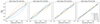 |
Fig. B.2. Equivalent to Fig. B.1, but for the mock MAHs. All figure elements are equivalent to the previous one. |
Each mock MAH is generated as follows:
-
We generate Na random numbers ui ∼ 𝒩(0, 1)+0.3, where 𝒩(0, 1) is a standardised normal distribution. This allows for the MAHs to locally decrease (as might be the case for actual halos), but also to present an overall increasing trend.
-
We obtain the cumulative sum,
 , and then smooth it with a Gaussian filter with σ = 2 points to get rid of small-scale oscillations.
 -
In order to reproduce the variability at the high-redshift end, we finally define the normalised MAH as:
 (B.3)
(B.3)
where x is yet another random number drawn from the 𝒩(0, 0.02) distribution. Empirically, we find that this heuristics produces curves with a shape remarkably similar to the real MAHs, as shown in Fig. B.3.
The PCA of the mock MAHs is shown in Fig. B.2, in a completely equivalent way to Fig. B.1 above for the real MAHs. Besides a slightly less smooth morphology in some cases, which can be attributed to the high-frequency noise in the mock MAHs, the mock data appears to distribute in a very similar way to the real one. Note that the only requirements imposed on these curves are:
-
Having a fixed extreme at a = 1 (ℳ = 1), and having an almost-fixed extreme at a ≃ 0.2 (ℳ ≪ 1).
-
Having an overall increasing trend, although decreasing intervals are allowed.
Therefore, it appears that these principal components, obtained by Wong & Taylor (2012) and which we reproduce in this work, are conceptually similar to the harmonic modes in a 1D system with the two fix boundary conditions. They emerge primarily as a consequence of these limiting behaviours of the MAH curves, namely lima → 1ℳ(a) = 1 and lima → astartℳ(a)≪1, and are probably not as much related to specific details about the whole span of the MAH (i.e. they do not seem to be related to possible physical properties, such as the typical timescale between mergers).
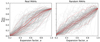 |
Fig. B.3. Comparison between the actual MAHs in our sample (left-hand side panel) and the mock ones generated to investigate the origin of their PCA (right-hand side panel). Here, gray lines are individual MAHs. The solid, red line is the mean MAH, while the dashed (dotted) lines indicate 32 − 68 (5 − 95) percentiles. |
This does not detract from the fact that the first two principal components are capable of explaining 77% (83% in Wong & Taylor’s 2012 case) of the variance in the (standardised) MAHs, implying that they constitute an idoneous base where to summarize their complex diversity. Indeed, as seen through Sect. 3.3 and especially in Fig. 8, the different indicators involved in this work seem to inform about different combinations of these two principal components, while other (perhaps more physically motivated) definitions aiming to summarise the MAHs do not allow us to extract as much information.
All Tables
Results summary for the timing analysis (central block) and the biparametric analysis (right-hand side block) on the MAHs, with each indicator given in each row.
Percentual mean relative error (MRE) between the tabulated MAHs of van den Bosch et al. (2014) and Correa et al. (2015), and the ones obtained from our simulation.
Fit parameters (α and β) for our three mass ranges to the functional form in Eq. (A.1).
All Figures
|
Fig. 1. Stacked mass assembly histories (MAHs) in three mass sub-samples, corresponding to galaxy clusters (light blue, thicker lines), high-mass groups (orange), and low-mass groups (turquoise, thinner lines). Dark shaded regions indicate the 1σ uncertainty around each mean MAH. Light shaded regions indicate the population standard deviation (just shown for the galaxy clusters sub-sample for clarity). Dashed (dotted) lines show the MAHs expected for each mass range according to the analytic (semi-analytic) model by Correa et al. (2015) (van den Bosch et al. 2014). |
| In the text | |
|
Fig. 2. Corner plot showing the univariate and bivariate distribution of the assembly state indicators and mass at R200m, all measured at z = 0. Along the diagonal, each panel presents the distribution of one variable, with the text in the top indicating the median value and (16, 84) percentiles. The sub-diagonal terms are scatter plots of the pair of variables indicated by the respective row and column. The text in magenta within each off-diagonal panel indicates the Spearman rank correlation coefficient between the corresponding pair of variables. The panels above the diagonal represent the same information as contours, for better visualisation in the densest parts. |
| In the text | |
|
Fig. 3. Effects of selecting halos based on their assembly state indicators at z = 0 on their full MAHs. Blue solid lines show the most relaxed third of the halo population at z = 0 according to each parameter, specified in the sub-plot title. Orange dashed lines refer to the most disturbed third. Dark and light contours indicate uncertainty on the mean and population scatter, respectively. The insets indicate the dependence of zform with the corresponding parameter, with a linear fit as the red, dashed line. |
| In the text | |
|
Fig. 4. Constraining power of the z0 = 0 assembly state indicators on the MAHs. Each panel shows the Spearman rank correlations between the MAH curves and a z0 = 0 assembly state indicator. The absolute magnitude of the curve at each z can be read as the fraction of the scatter on the ranking of M(z)/M0 that can be explained by the corresponding parameter at z0 = 0. The green regions indicate the redshift intervals where this correlation exceeds 0.3 in magnitude, with the green, vertical lines delimiting the interval to ease the visualisation. The horizontal, grey, dashed line marks null correlation. The arrows indicate the redshift at which this correlation is maximal, zc, X. |
| In the text | |
|
Fig. 5. Impact of accretion rates on each of the z0 = 0 assembly state indicators. Each panel shows the Spearman rank correlations between the instantaneous MARs and an assembly state indicator at z0 = 0. All plot elements are equivalent to Fig. 4. |
| In the text | |
|
Fig. 6. Impact of accretion rates on each of the z = 0.5 (indicated as a vertical, grey, dashed line) assembly state indicators. All plot elements are equivalent to Fig. 5. |
| In the text | |
|
Fig. 7. Parametrisation of the MAHs. The two top panels present the assembly histories of the whole sample, colour-coded according to the formation redshift zform (left) and the episodicity parameter αMAH (right-hand side panel). The two bottom panels describe the distribution of these parameters in the {PC1, PC2} space, accounting for the maximum variance with two linearly uncorrelated components. The colour coding of the dots is the same as represented in their respective top panels. |
| In the text | |
|
Fig. 8. Constraints of the assembly state indicators on the two biparametric characterisations of the MAHs: the zform − αMAH plane (top panel) and the PC1 − PC2 plane (bottom panel). In each panel, the different arrows correspond to each of the assembly indicators according to the colour legend in the bottom panel. Their directions indicate the relative weight of each of the two parameters in the linear combination which best correlates with the given indicator, while their magnitude is the Spearman rank correlation coefficient between the indicator and the corresponding projection of the MAH representation (the larger, the more information is yielded by the indicator). Colour aid: Arrows correspond to χ, Δr, fsub, λBullock, |
| In the text | |
|
Fig. 9. Assembly histories for individual clusters (summarised in the PC1 − PC2 plane) colour-coded according to each of the assembly state indicators at z = 0. The colour bars are ordinal (i.e. linear in the ranked variable: e.g. the middle point of the colorbar corresponds to the median value). At the top of each panel, we indicate the direction of maximum correlation with the indicator, the Spearman rank correlation coefficient, and the Kendall rank correlation coefficient. |
| In the text | |
|
Fig. 10. Correspondence between the assembly state indicators measured from the DM distribution (horizontal axes) and from the ICM distribution (vertical axes), at z = 0. Each panel corresponds to a different parameter. Within each panel, each dot corresponds to a cluster or group; the dashed, gray line is the identity relation (Xgas = XDM); and the dashed red line is a least-squares linear fit, whose slope (m) is given at the top of each panel. Also the Spearman and Kendall rank correlation magnitudes, and their p-values, are given there. |
| In the text | |
|
Fig. A.1. Equivalent to Fig. 1 of the main text, with the main branch of the merger tree having been set by choosing the most massive progenitor at each timestep. |
| In the text | |
|
Fig. B.1. First four principal components of our MAHs (from left to right, in decreasing order of explained variance, stated in the title of each panel). Within each panel, the black line represents the mean MAH of the sample. The different additional curves correspond to ±1σ and ±2σ of the values of the corresponding principal component, reflecting how each component is producing changes in the MAHs of our sample. |
| In the text | |
|
Fig. B.2. Equivalent to Fig. B.1, but for the mock MAHs. All figure elements are equivalent to the previous one. |
| In the text | |
|
Fig. B.3. Comparison between the actual MAHs in our sample (left-hand side panel) and the mock ones generated to investigate the origin of their PCA (right-hand side panel). Here, gray lines are individual MAHs. The solid, red line is the mean MAH, while the dashed (dotted) lines indicate 32 − 68 (5 − 95) percentiles. |
| In the text | |
Current usage metrics show cumulative count of Article Views (full-text article views including HTML views, PDF and ePub downloads, according to the available data) and Abstracts Views on Vision4Press platform.
Data correspond to usage on the plateform after 2015. The current usage metrics is available 48-96 hours after online publication and is updated daily on week days.
Initial download of the metrics may take a while.