| Issue |
A&A
Volume 688, August 2024
|
|
|---|---|---|
| Article Number | A184 | |
| Number of page(s) | 21 | |
| Section | Stellar structure and evolution | |
| DOI | https://doi.org/10.1051/0004-6361/202449882 | |
| Published online | 21 August 2024 | |
Asteroseismic measurement of core and envelope rotation rates for 2006 red giant branch stars
1
IRAP, Université de Toulouse, CNRS, CNES, UPS, 14 avenue Edouard Belin, 31400 Toulouse, France
2
Institute of Astronomy, KU Leuven, Celestijnenlaan 200D, 3001 Leuven, Belgium
Received:
6
March
2024
Accepted:
20
May
2024
Context. Tens of thousands of red giant stars in the Kepler data exhibit solar-like oscillations. The mixed-mode characteristics of their oscillations enable us to study the internal physics from the core to the surface, such as differential rotation. However, envelope rotation rates have only been measured for about a dozen red giant branch (RGB) stars so far. This limited the theoretical interpretation of angular momentum transport in post-main sequence phases.
Aims. We report the measurements of g-mode properties and differential rotation in the largest sample of Kepler RGB stars.
Methods. We applied a new approach to calculate the asymptotic frequencies of mixed modes, which accounts for so-called near-degeneracy effects (NDEs) and leads to improved measurements of envelope rotation rates. By fitting these asymptotic expressions to the observations, we obtained measurements of the properties of g modes (period spacing, ΔΠ1, coupling factor, q, g-mode offset term, εg, small separation, δν01) and the internal rotation (mean core, Ωcore, and envelope, Ωenv, rotation rates).
Results. Among 2495 stars with clear mixed-mode patterns, we found that 800 show doublets and 1206 show triplets, while the remaining stars do not show any rotational splittings. We measured core rotation rates for 2006 red giants, doubling the size of pre-existing catalogues. This led us to discover an over-density of stars that are narrowly distributed around a well-defined ridge in the plane, showing core rotation rate versus evolution along the RGB. These stars could experience a different angular momentum transport compared to other red giants. With this work, we also increased the sample of stars with measured envelope rotation rates by two orders of magnitude. We found a decreasing trend between envelope rotation rates and evolution, implying that the envelopes slow down with expansion, as expected. We found 243 stars whose envelope rotation rates are significantly larger than zero. For these stars, the core-to-envelope rotation ratios are around Ωcore/Ωenv ∼ 20 and show a large spread with evolution. Several stars show extremely mild differential rotations, with core-to-surface ratios between 1 and 2. These stars also have very slow core rotation rates, suggesting that they go through a peculiar rotational evolution. We also discovered more stars located below the ΔΠ1–Δν degeneracy sequence, which presents an opportunity to study the history of plausible stellar mergers.
Key words: stars: interiors / stars: oscillations / stars: rotation / stars: solar-type
© The Authors 2024
 Open Access article, published by EDP Sciences, under the terms of the Creative Commons Attribution License (https://creativecommons.org/licenses/by/4.0), which permits unrestricted use, distribution, and reproduction in any medium, provided the original work is properly cited.
This article is published in open access under the Subscribe to Open model. Subscribe to A&A to support open access publication.
1. Introduction
Thanks to the advent of recent space-based photometric missions, particularly the Kepler mission (Borucki et al. 2010), it has been possible to observe stellar oscillations with a level of precision that was previously unimaginable through ground-based observations. One remarkable achievement in the field of asteroseismic research is related to red giants, which are stars that have depleted their central hydrogen and are now burning hydrogen in the shell. The oscillations in red giants are stochastically excited in the outer convective envelope, which is similar to the Sun. To date, tens of thousands of solar-like oscillators have been discovered by Kepler (Bedding et al. 2010; Yu et al. 2018).
The power spectra of solar-like oscillators exhibit distinct regular-spaced radial (l = 0) and quadrupole (l = 2) modes, where l represents the angular degree. In post-main sequence solar-like stars, dipole (l = 1) modes show a mixed-mode nature. This arises from the coupling between the outer pressure modes and the interior gravity modes (Bedding 2014). Unlike the equally spaced frequencies or periods predicted by the asymptotic relation (Shibahashi 1979; Tassoul 1980), the frequencies of mixed modes display a more complex pattern (e.g., Goupil et al. 2013; Mosser et al. 2012b, 2015). The coupling between the stellar interior and outer envelope allows us to investigate the physics from the stellar core to the surface. For example, mixed modes have been used to distinguish between hydrogen-shell-burning and helium-core-burning giants (Bedding et al. 2011) and unveil indications of mass transfer or merger (Deheuvels et al. 2022; Rui & Fuller 2021; Tayar et al. 2022; Li et al. 2022b). Mixed modes are predicted to reveal central magnetic fields, as these fields lead to frequency shifts (Gomes & Lopes 2020; Loi 2021; Bugnet et al. 2021; Mathis et al. 2021; Li et al. 2022a; Mathis & Bugnet 2023), modifications in period spacing (Loi 2020; Li et al. 2022a; Bugnet 2022; Deheuvels et al. 2023), and amplitude suppression (Fuller et al. 2015; Stello et al. 2016; Mosser et al. 2017a; Loi & Papaloizou 2017, 2018). The intensities and topology of central magnetic fields in dozens of stars have been reported by Li et al. (2022a, 2023), and Deheuvels et al. (2023).
Pertinent to the interests of this work, mixed modes can also be used to measure the internal rotation rates of red giant stars, most of which are core rotation rates (Beck et al. 2012; Gehan et al. 2018; Kuszlewicz et al. 2023). As a contrast, the envelope rotation rates have only been reported for dozens of stars (Deheuvels et al. 2012, 2014; Di Mauro et al. 2016; Triana et al. 2017).
Stellar rotation plays a crucial role in the process of stellar evolution (Maeder 2009). It leads to the distortion of stellar structure and facilitates the transport of additional hydrogen to the core, thereby extending the star’s lifetime. Asteroseismology offers a powerful method for accurately measuring rotation rates in different depths of a star. Studies have revealed that main sequence stars (not only Sun-like stars, including the Sun itself, but also hotter γ Doradus stars: A to F type), show nearly uniform rotations (Schou et al. 1998; Gough 2015; Benomar et al. 2015; Nielsen et al. 2015; Li et al. 2020b; Aerts et al. 2019). The rotation periods of main sequence stars decrease with increasing masses, ranging from tens of days to one day, consistent with spectroscopic observations (Royer et al. 2007; McQuillan et al. 2014; Van Reeth et al. 2016; Li et al. 2020b; Saio et al. 2021). After the main sequence, stars tend to rotate differentially. Deheuvels et al. (2014, 2020) found a clear transition from near-uniform to differential rotations in young subgiant stars. Afterwards, the core rotation rates of red giants show no correlation with their evolution and mass, even though their cores are contracting, which implies that some additional, efficient angular momentum transport mechanisms are at work (Mosser et al. 2012a; Wu et al. 2016; Gehan et al. 2018). As stars evolve beyond the red giant branch (RGB) stage and enter the helium-burning phases, the amount of differential rotation decreases (Deheuvels et al. 2015).
Despite its recognised importance, the theoretical understanding of angular momentum transport remains a primary challenge in current stellar physics. Firstly, rotation rates are consistently slower than predicted at nearly all stages of stellar evolution (Ouazzani et al. 2019; Li et al. 2020b; Fuller et al. 2019). Secondly, the pure hydrodynamic processes that involve angular momentum transfer through meridional circulation and shear instabilities (e.g. Zahn 1992; Mathis & Zahn 2004; Mathis et al. 2018) generate excessively strong differential rotation, which is not supported by observations (e.g. Eggenberger et al. 2012; Ceillier et al. 2013; Marques et al. 2013). These discrepancies imply the existence of unknown mechanisms responsible for internal angular momentum transport within stars. The efficiency of these mechanisms was found to increase with stellar mass and evolution on the red giant branch (Cantiello et al. 2014; Eggenberger 2015; Spada et al. 2016). By contrast, it was shown that the efficiency of angular momentum transport decreases with evolution during the subgiant phase (Eggenberger et al. 2019).
Several mechanisms have been proposed to reconcile the discrepancy between theoretical predictions and observations. One such mechanism involves internal gravity waves (IGW) that are excited at the base of the convective envelope and contribute to additional angular momentum transport (Fuller et al. 2014; Pinçon et al. 2016). However, IGWs still face challenges in explaining the rotational behaviour of more evolved red giants. Mixed modes, on the other hand, could be efficient at transporting angular momentum on the upper RGB (Belkacem et al. 2015). Recently, core magnetic fields were discovered in some red giant stars (Li et al. 2022a, 2023; Deheuvels et al. 2023), providing observational constraints on how magnetic fields influence angular momentum transport (e.g. Maeder & Meynet 2014; Kissin & Thompson 2015; Rüdiger et al. 2015; Jouve et al. 2015; Fuller et al. 2019; Barrère et al. 2023; Petitdemange et al. 2023, 2024). Recently, Eggenberger et al. (2022a) showed the importance of the Tayler instability in the Sun to reproduce the observed internal rotation profile and lithium and helium abundances. Angular momentum transport via the Tayler instability appears to better match the asteroseismic core rotation rates of both main-sequence and post-main sequence stars (Moyano et al. 2023; Eggenberger et al. 2022b). However, theories based on magnetism still struggle to fully explain the observed internal rotations. Another important mechanism to consider is binary interaction. It has been demonstrated that tidal effects from binary companions can significantly shape the internal rotations of stars (Li et al. 2020a; Fuller 2021; Ahuir et al. 2021). Given the prevalence of binary systems, the tidal effects they induce cannot be ignored and may have a substantial impact on stellar rotation.
Current studies typically report only the core rotation rates of RGB stars, operating under the assumption that the envelope rotation rates are negligible and can be treated as zero. There are samples of roughly one thousand stars whose core rotation rates have been measured (Gehan et al. 2018; Kuszlewicz et al. 2023). Conversely, a limited number of red giants, approximately twenty, have had their envelope rotation rates directly measured (Deheuvels et al. 2014; Di Mauro et al. 2016; Triana et al. 2017). This type of measurement is complicated for several reasons. First, the strong expansion of red-giant envelopes causes them to spin down, so the envelope rotation periods are long and become comparable to the duration of Kepler observations for more evolved red giants. Secondly, while rotation inversions are very efficient at providing estimates of core rotation rates, they can lead to biased measurements for the envelope rotation rates because of the pollution from the core (Deheuvels et al. 2014). This is all the more true for evolved giants. Finally, as we show in the present paper, the measurements of envelope rotation rates can be strongly affected by the so-called near-degeneracy effects (NDE), which arise when the frequency separation between consecutive mixed modes is comparable to the rotational splitting (Deheuvels et al. 2017). None of the studies performed so far to measure the internal rotation of red giants using dipole mixed modes accounted for these NDE.
In the present work, we have analysed existing seismic observations of red giant stars obtained by the Kepler mission to measure both the core and envelope rotation rates for a large number of targets. We thus treated the envelope rotation rates as free parameters and investigated whether we can effectively constrain their values. We introduced a new fitting method based on the asymptotic expression of mixed modes, which can properly account for NDE. Finally, we were able to significantly expand the sample of RGB stars with measured internal rotation: the sample size has been doubled for core rotation rates and multiplied by a factor of 100 for envelope rotation rates.
The paper is organised as follows: In Section 2, we introduce asymptotic expressions of mixed modes, which are then fit to the observed spectra. We propose a new method that avoids using the ζ function and we show that it is better suited to measure envelope rotation rates in Section 3.1. We compare our results with the previous literature in Section 3.2 and show that our results are generally consistent and reliable. In Section 4, we present our results and comment on the distributions that we obtain for core and envelope rotation rates, and their dependence on stellar parameters. Special care is given to stars that might undergo a process of mass transfer or merger. Finally, the conclusions are given in Section 5.
2. Data analysis
2.1. Sample collection
We collected the red giant stars from the catalogues by Yu et al. (2018) and Gehan et al. (2018) and used the Kepler four-year long-cadence data downloaded from the Mikulski Archive for Space Telescopes (MAST) to perform the seismic analysis. We derived the frequency of the maximum power (νmax), the initial estimate of the large frequency separation (Δν), and the Harvey background (Karoff 2008) by applying the algorithm used in the SYD pipeline (Huber et al. 2009; Chontos et al. 2021).
2.2. Asymptotic properties of pressure modes
Before fitting the l = 1 mixed modes, we need to obtain information on the asymptotic properties of p modes. Quadrupole modes are in principle mixed modes. However, since the coupling between the p- and g-mode cavities is much weaker for these modes that for dipole modes, only l = 2 modes that behave predominantly as p modes are visible. The frequencies of l = 0 and l = 2 modes (νp) are derived by fitting the oscillation spectrum with the Lorentzian profiles, which are written as
where P(ν) is the oscillation power, a0 is the amplitude parameter, ν0 is the centre of the profile, and η is the half width at half maximum. For each star, we ran a Markov chain Monte Carlo (MCMC) optimisation algorithm to search for the best-fitting results using the emcee package (Foreman-Mackey et al. 2013). In the MCMC algorithm, we maximised the likelihood function, defined by Anderson et al. (1990) as
![$$ \begin{aligned} \ln p\left(D|\theta , M \right) = -\sum _i\left[\ln M_i\left(\theta \right) +\frac{D_i}{M_i\left(\theta \right)} \right], \end{aligned} $$](/articles/aa/full_html/2024/08/aa49882-24/aa49882-24-eq2.gif)
where Di is the observed data, θ stands for the parameters, and Mi is the model. In this MCMC algorithm, we obtained the best-fitting frequencies for l = 0 and l = 2 modes  and their uncertainties
  .
.
For high-radial order p modes, the second-order asymptotic relation can be expressed as
where Δν is the revised large separation, εp is the p-mode phase term, and nmax = νmax/Δν is the radial order at the max-power frequency (Mosser et al. 2012b). The term D describes the small separation between l = 0 and 2 modes (Shibahashi 1979; Tassoul 1980; Mosser et al. 2011).
We ran another MCMC optimisation algorithm to obtain the best-fitting Δν, εp, α, and D by maximising the likelihood function Lp defined as:
![$$ \begin{aligned} \ln L_\mathrm{p} = -\frac{1}{2} \sum _{l=0,2}\sum _{i} \left[ \frac{\left(\nu _{l, i}^\mathrm{obs} -\nu _{l, i}^\mathrm{cal} \right)^2}{\sigma _{l, i}^2} +\ln \left(2\pi \sigma _{l, i}^2\right) \right], \end{aligned} $$](/articles/aa/full_html/2024/08/aa49882-24/aa49882-24-eq6.gif)
where  is the ith observed frequencies of l = 0 and l = 2 modes,
  is the theoretical frequencies calculated by Eq. (3), and σl, i is the uncertainty. After fitting all the stars’ p modes, we find that there is a residual spread with a median value σm = 0.042 μHz. We consider that this value σm is the model error due to the limitation of the asymptotic relation Eq. (3). To properly account for it, the uncertainty of p-mode frequency is defined as a quadratic summation as
In the MCMC code, we used 32 parallel chains and 2000 steps, retaining only the last 1600 steps as the final posterior distributions. The asymptotic expression of the p modes is simple and explicit, allowing the MCMC code complete its task and converge rapidly.
2.3. Asymptotic expression for l = 1 mixed modes
After fitting and removing the l = 0 and l = 2 p modes, We followed the so-called ‘stretched echelle diagram’ procedure introduced by Mosser et al. (2015) to extract the l = 1 mixed modes and identify their azimuthal orders m. In this procedure, the unevenly-spaced l = 1 mixed modes are stretched by a differential equation to generate vertical ridges in the stretched échelle diagram. The vertical ridges provide the estimate of the period spacing ΔΠ1, and the slight differences in the period spacings found for the ridges allow us to identify their azimuthal orders m. Figure 1 shows a stretched échelle diagram using KIC 8636389 as an example.
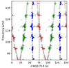 |
Fig. 1. Stretched échelle diagram of KIC 8636389. The x-axis is the stretched period τ module of 75.9 s. The y-axis is the oscillation frequency. The grey dots are the peaks with S/N higher than 10. The blue circles are identified as l = 1 m = 0 mixed modes. The red line and green plus are the m = −1 and m = +1 modes. The crosses show the best-fitting frequencies. |
To calculate the asymptotic frequencies of l = 1 mixed modes (Shibahashi 1979, Unno et al. 1989), we solve the equation:
where q is the coupling factor, which gives physical constraints on the regions surrounding the radiative core and the hydrogen-burning shell of subgiants and red giants (Mosser et al. 2017b). θg and θp are phase terms characterising pure g and p modes, given by
and
The frequencies νg of pure l = 1 g modes are equally spaced in period, and hence can be written as
where εg is an offset term. Here, we adopt the same definition of εg as Mosser et al. (2015). However, as discussed by Lindsay et al. (2022) and Ong & Gehan (2023), with this definition, Eq. (6) fails to recover the frequencies of pure g modes in the case of a weak coupling (when q → 0). We caution the reader that there is a  offset of εg in our work, so
  should be the correct value of εg using the proper definition.
The terms νp, l = 1 in Eq. (8) are the frequencies of l = 1 pure p modes. They cannot be calculated directly from Eq. (3) because the small separation δν01 (the amount by which l = 1 modes are offset from the midpoint of consecutive l = 0 modes, Bedding 2014) varies with evolution and cannot be reproduced well using only the D parameter (Lund et al. 2017). Therefore, we include an additional free parameter fshift to describe the shift of the l = 1 pure p modes, as
The parameter fshift is related to the small separation  . Ignoring the second-order term, we have δν01 = 2D − fshift. We provide a discussion about the small separation δν01 in Appendix B.
2.4. Rotational perturbation
To take into account the rotational perturbations to mixed mode frequencies, we attempted two different approaches and we will show that the second approach is a better way.
2.4.1. Approach one
Approach one is the commonly-used method used to calculate the rotational splittings δνrot of mixed modes in red giants. It is now customary to follow Goupil et al. (2013) and to express it as
where Ωcore is the average core rotation, Ωenv is the average envelope rotation, and ζ is the ratio of mode inertia in the g cavity over the total mode inertia, hence ζ = 1 stands for a pure g mode while ζ = 0 is pure p modes (Deheuvels et al. 2012; Goupil et al. 2013). This expression is particularly convenient because the function ζ(ν) can be expressed as a function of the asymptotic properties of pure p and g modes as (Mosser et al. 2015; Gehan et al. 2018)
![$$ \begin{aligned} \zeta = \left[1+\frac{\nu ^2}{q}\frac{\Delta \Pi _1}{\Delta \nu }\frac{1}{\frac{1}{q^2}\sin ^2\theta _\mathrm{p} +\cos ^2\theta _\mathrm{p} }\right]^{-1}. \end{aligned} $$](/articles/aa/full_html/2024/08/aa49882-24/aa49882-24-eq19.gif)
Thus, the frequencies of m = 0 modes νm = 0 can be first obtained by solving Eq. (6), and the frequencies of m = ±1 modes can then be calculated as νm = ν0 − mδνrot. The advantages of this approach are that the best-fitting result provides the splitting identification even though the splittings overlap each other, and the computation is relatively fast since the ζ function is explicit.
The disadvantage of approach one is the lack of consideration of near-degeneracy effects (NDE). NDE arise when the frequency separation between consecutive mixed modes is comparable to or lower than the rotational splitting. They generally lead to asymmetries in the rotational multiplets of p-dominated mixed modes (Deheuvels et al. 2017). As stars evolve along the RGB, we expect NDE to become more important because their asymptotic period spacing decreases. Also, NDE are naturally larger for stars with faster-rotating cores. Approach one uses the ζ function to obtain approximate expressions for the rotational splittings (Eq. (6)) and therefore has symmetric rotational multiplets by construction. For stars that show non-negligible NDE, approach one inadequately captures the structure of p-dominated modes, which can lead to biases in the measurements of the envelope rotation Ωenv and the coupling factor q.
2.4.2. Approach two
Approach two consists of including rotational perturbations to the asymptotic frequencies of pure p- and g-modes before accounting for the coupling between the cavities. These frequencies are thus expressed as
and
They are then used to calculate the perturbed g and p phase terms for m = 1, 0, −1 as
and
After this, the implicit function for m = 1, 0, and −1 is solved three times to obtain the frequencies with different m values:

Solving Eq. (17) is much more time-consuming than approach one since it is implicit, but we argue below that it provides a more reliable solution. We note that approach two has already been used by Li et al. (2022a, 2023), and Deheuvels et al. (2023), but these works also included magnetism-induced perturbations. Here we only consider rotational perturbations.
Approach two is in fact similar to the one proposed by Ong et al. (2022) to account for the NDE. Starting from the oscillation operator perturbed by rotation, the authors isolate pure pressure modes (π modes) and pure gravity modes (γ modes). Then, they decompose the mode eigenfunctions in the basis of isolated π and γ modes and they argue that the rotation operator is diagonal in this representation. This shows that in this basis, the effects of rotation on the mode frequencies can indeed be separated from the effects of the coupling, as we have done in approach two. Ong et al. (2022) showed that they obtained the same expressions as the ones that were found by Deheuvels et al. (2017) to account for the NDE. The only difference between the approach of Ong et al. (2022) and our approach two is that the latter uses WKB expressions of mode frequencies, while the former uses eigenfrequencies and eigenfunctions numerically computed with a code solving the unperturbed set of oscillation equations. We thus expect approach two to adequately account for the NDE, contrary to approach one.
2.5. MCMC optimisation for mixed modes
We ran an MCMC optimisation algorithm to search for the best-fitting parameters of l = 0, l = 2, and l = 1 frequencies. Table 1 lists all the ten parameters that were optimised, along with their ranges of uniform priors. The top four parameters describe the p-mode asymptotic expression in Eq. (3), while the rest six parameters describe the mixed modes. The likelihood function for l = 1 mixed modes is defined as:
![$$ \begin{aligned} \ln L_{l=1} = -\frac{1}{2}\sum _{m=1, 0, -1} \sum _i\left[\frac{\left(\nu _{m, i}^\mathrm{obs} -\nu _{m, i}^\mathrm{cal} \right)^2}{\sigma _{m, i}^2} +\ln \left(2\pi \sigma _{m, i}^2\right)\right], \end{aligned} $$](/articles/aa/full_html/2024/08/aa49882-24/aa49882-24-eq25.gif)
where  and
and  are the observed and calculated ith frequencies with azimuthal order m, and σm, i is the uncertainty of the ith frequency with azimuthal order m.
We followed a two-step procedure. In the first step, we ran the MCMC optimisation code with fixed p-mode parameters and constant uncertainties  for l = 1 mixed mode frequencies. At this point, we considered the points with a S/N higher than ten as input frequencies. The best-fitting results helped us identify the rotational splittings of l = 1 mixed modes. We then fitted Lorentzian profiles on them, which allowed us to derive proper estimates of the mode frequencies and their related uncertainties
  . Figure C.1 shows an example of the result of the Lorentzian fit for a star of the sample. Beside the central frequency, this fitting procedure also provides estimates of the rotational splittings, δνrot, the stellar inclination, i, the mode amplitude, a0, and linewidths, η, and the background of the power spectrum.
In the second step, we re-ran the MCMC code using the frequencies and uncertainties acquired through the Lorentzian fit. This step enabled us to accurately estimate the uncertainties of the parameters related to the asymptotic expressions of the modes. We then treated the p-mode parameters as free parameters, incorporating them into the MCMC process alongside the mixed-mode parameters. We found that our best-fitting models have a residual spread, whose median is larger when |θp|< 0.15π (corresponding to p-dominated modes) and smaller when |θp|> 0.15π (which are g-dominated modes). We indeed found a median σp = 14 nHz for p-dominated modes, and σg = 7 nHz for g-dominated modes. We consider this residual spread as the model uncertainty of the asymptotic expressions. The larger residual on p-dominated modes might be a hint of small glitches, which influence our estimation of envelope rotation rates. To include the model uncertainty properly, we define the frequency uncertainty as
![$$ \begin{aligned} \begin{split}&\sigma _{m, i} = \left[ \sigma _{\rm p}^2+ \left(\sigma _{m, i}^\mathrm{obs} \right)^2 \right]^{0.5}~\mathrm{when} ~|\theta _\mathrm{p} | < 0.15\pi , \\&\mathrm{or} \\&\sigma _{m, i} = \left[ \sigma _{\rm g}^2+ \left(\sigma _{m, i}^\mathrm{obs} \right)^2 \right]^{0.5}~\mathrm{when} ~|\theta _\mathrm{p} |>0.15\pi , \end{split} \end{aligned} $$](/articles/aa/full_html/2024/08/aa49882-24/aa49882-24-eq30.gif)
where  is the observed frequency uncertainty from the Lorentzian profile fitting. To fit p modes and mixed modes together, the likelihood function is defined as the sum of Eqs. (18) and (4), that is
The MCMC code for mixed mode is more time-consuming. We used 22 parallel chains and 6000 steps, and we discarded the first half of the chain to obtain the posterior distributions. This choice ensures both MCMC convergence and time cost. We also visually inspected all the results of stars to ensure that the chains were well converged and their posterior distributions did not reach the boundary of their uniform priors. In some cases, we found that εg reached its boundary (the initial one is −0.1 < ε < 1.1), so we just set a larger boundary for the uniform prior of εg.
Here we show KIC 9289599 as an example, which is selected randomly from our sample. Figure 2 displays the corner diagram of the MCMC fit using approach two, which demonstrates that the chain converges well. We find that there is a strong anti-correlations between ΔΠ1 and εg, which can be understood from Eq. (9) as the product ΔΠ1εg plays a holistic role. The core and envelope rotation rates (Ωcore and Ωenv) also show anti-correlations. This is because the sum of the two rates, weighted by the ζ function, determines the magnitude of the rotational splitting. Some correlations between p-mode parameters and g-mode parameters are also found, such as the correlation between ΔΠ1 and Δν, which can be understood in Eq. (6).
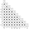 |
Fig. 2. Corner diagram of the posterior distributions of KIC 9289599 by approach two. |
2.6. Sample and selection effects
During the visual inspection of our stars, we removed the stars that show glitches caused by the discontinuity in the cores (Cunha et al. 2015) and also the stars showing curved stretched échelle diagrams or asymmetric rotational splittings which are caused by their central magnetic fields (Li et al. 2022a, 2023; Deheuvels et al. 2023). In total, we collected 2495 stars that show clear l = 1 mixed-mode patterns. The 2006 stars show rotational splittings hence the ten parameters (Table 1) including the core and the envelope rotation rates are measured. Among them, 800 stars show doublets and 1206 stars show triplets. However, 489 stars show only l = 1, m = 0 modes. In these cases, we could not measure their internal rotations, so we only measured the eight other parameters. In solar-like oscillations, the relative amplitudes of the components in rotational splittings are determined by the inclination of the rotational axis (Gizon & Solanki 2003). Inclination close to 0° leads to the visibility of m = 0 modes while a 90° inclination allows m = ±1 modes to be visible. Intermediate inclinations generate triplets. We also measured the inclinations of our sample, which are discussed in Appendix B. All the 2495 stars were inspected to assure that the best-fitting results are correct. During the inspection, we concentrated on evaluating the following points: 1) whether the fit residuals are small; and 2) whether the MCMC algorithm converged properly. The main issues with the above two points are primarily related to mode identifications, such as failing to correctly identify the large frequency separation, mistaking l = 3 modes for l = 1 mixed modes, or encountering issues while fitting the Lorentzian profile for rotational splitting. These problems could all be manually corrected.
Figure 3 displays the distributions of Δν and stellar mass of our sample and the sample by Yu et al. (2018). For the Δν distribution in the top panel of Fig. 3, we observe a distinct cut-off at around Δν ≈ 7.5 μHz. Below this value, the mixed modes are unclear due to the short mode lifetime caused by the radiative damping (Grosjean et al. 2014), hence it is hard to identify any pattern. We find that our Δν cut-off of ∼7.5 μHz is larger than what is predicted by Grosjean et al. (2014), which is 4.9 μHz. The bottom panel of Fig. 3 displays the distribution of stellar mass in our sample and the sample by Yu et al. (2018). The masses of the stars in our sample predominantly range from approximately ∼0.7 to 2.0 M⊙. The fraction of stars exhibiting clear mixed-mode pattern increases with masses, and reaches the maximum around 1.25 M⊙, where about 30% stars are included in our sample. Subsequently, the fraction gradually decreases, reaching around 5% at M ≈ 2.0 M⊙. The scarcity of high-mass stars could be attributed to the suppression of l = 1 modes induced by central magnetic fields, whose prevalence increases with increasing stellar mass (Stello et al. 2016).
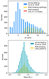 |
Fig. 3. Distributions of Δν (top) and mass (bottom) of our sample and the sample by Yu et al. (2018). |
3. Comparison of results
3.1. Approach one versus approach two
We compared the results given by the two different approaches used to compute the rotational splitting of mixed modes in Sects. 2.4.1 and 2.4.2. These two approaches show general consistency for the estimates of all parameters but one, the average envelope rotation rate Ωenv. As shown in the two panels of Fig. 4, approach one (left panel) tends to yield significantly negative rotation rates of the envelopes. This is particularly the case when Δν < 11 μHz, that is, for more evolved giants. In contrast, approach two (right panel of Fig. 4) does not exhibit any spread of Ωenv for stars with small Δν.
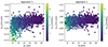 |
Fig. 4. Envelope rotation rates derived by approaches one and two. The colour bar indicates the intensity of NDE, calculated as the ratio between the core rotation and Δfmin, which is the smallest frequency separation between consecutive l = 1 mixed modes around νmax (see Sect. 3.1). |
In Fig. 5, we show the differences obtained between approach one and two for core and envelope rotation rates. The left panel of Fig. 5 shows that there is a slight but significant systematic deviation in the core rotation rates, particularly at smaller values of Δν. At Δν ≈ 8 μHz, the core rotation rates given by approach two are on average smaller than those given by approach one by about 10 nHz. However, this difference diminishes as Δν increases. Regarding the envelope rotation rates (right panel in Fig. 5), the two approaches show a systematic deviation, accentuated at small values of Δν by the subset of stars that are found to have large negative rotation rates with approach one.
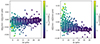 |
Fig. 5. Differences of the core and envelope rotation rates between approaches two and one (defined as the results from approach two minus the results from approach one). The colour bar represents the extent of the NDE (see Fig. 4 and Sect. 3.1). The horizontal dashed lines mark the location where the values are equal. The white error bars show the mean and standard deviations in each bin of Δν. |
We suspected that these differences were caused by the NDEs. To verify this, we estimated the intensity of the NDE that is expected in the targets of our sample. For this purpose, we calculated the smallest frequency separation Δfmin between consecutive mixed modes around νmax and we compared this quantity to the core rotation rate Ωcore/(2π). NDE become important when the ratio Ωcore/(2πΔfmin) becomes of the order of unity or more. In Figs. 4 and 5, the points are colour-coded with the value of this ratio. It appears clearly that the stars that are found to have large negative envelope rotation rates with approach one correspond to stars for which large NDE are expected. Conversely, when using approach two, stars with large NDE have envelope rotation rates that are similar to those of other stars (right panel of Fig. 5).
As an additional verification that approach two adequately captures NDE, we considered a reference star for which NDE are expected to be non-negligible and approach one reports a large negative envelope rotation rate (we picked KIC 11245496, for which Ωcore/(2πΔfmin) = 2.4). We computed a stellar model approximately representative of this star (showing similar values of Δν and ΔΠ1) with the MESA code (Paxton et al. 2011) and we calculated its mode frequencies and eigenfunctions with ADIPLS (Christensen-Dalsgaard 2008). To estimate the rotational perturbation to the mode frequencies accounting for NDE in this model, we followed Deheuvels et al. (2017) to generate synthetic frequencies (see Appendix E). Significant multiplet asymmetries arise in the vicinity of p-dominated modes owing to NDE, as can be seen in Fig. 6. We then considered the perturbed frequencies of this model as mock observations and attempted to fit them using approach two. The results are shown in Fig. 6, where it can be seen that the asymmetries of multiplets are very well reproduced using approach two (for comparison, we recall that the asymmetries are by construction equal to zero when using approach one). Also, the parameters recovered when using approach two (in particular the core and envelope rotation rates) are in good agreement with the input values. This confirms that approach indeed accounts well for NDE. In Fig. A.1, we present the observed splitting asymmetries and the best-fitting results of KIC 11245496. We claim that approach two indeed can reproduce the observed splitting asymmetries.
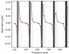 |
Fig. 6. Synthetic asymmetries in l = 1 rotational multiplets resulting from near-degeneracy effects in KIC 11245496. The red dots are the simulated asymmetries following the method by Deheuvels et al. (2017), while the grey dots and lines are the best-fitting results by approach two. The background shows the ζ values: the darker, the smaller, hence the dark fringes stand for the positions of p-dominated modes. |
3.2. Comparison with previous works
We selected the stars that were also studied by Gehan et al. (2018) and Mosser et al. (2018) and compared the parameters obtained in our work with those from the previous studies. In Fig. 7, we present the comparison between the results obtained using approach two and the previous studies.
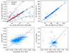 |
Fig. 7. Comparison between our result with previous studies. Top left: core rotation rate Ωcore. Top right: period spacing ΔΠ1. Bottom left: coupling factor q. Bottom right: g-mode phase εg. the dashed line in each panel shows the 1:1 relation, or 2:1 and 1:2 as marked. |
In the top left panel of Figure 7, we present the comparison of the core rotation rates (Ωcore) between our results and those from Gehan et al. (2018). For this comparison, we selected a total of 693 stars that are studied in both works. In general, the measurements of core rotation rates show good agreement between the two studies, indicating consistency. However, we do observe a small fraction of stars where the core rotation rates obtained in our study are approximately twice those reported by Gehan et al. (2018). To be specific, there are 32 stars that Gehan et al. (2018) reported larger core rotation rates (ΔΩcore/2π larger than 0.1 μHz), while 61 stars were reported smaller core rotation rates by Gehan et al. (2018; ΔΩcore/2π smaller than 0.1 μHz). This discrepancy could be attributed to the misidentification of the azimuthal order m in these particular stars. As plotted by the grey downward-pointing triangles in the upper left panel of Figure 7, a significant portion of stars that fall along the 2:1 trend exhibit triplets in their rotational splittings. It is plausible that the previous study misidentified these triplets as doublets, failing to recognise one of the components, consequently leading to the calculation of core rotation rates at half their actual values. Additionally, we find several stars in our sample that exhibit smaller rotation rates compared to the measurements reported in Gehan et al. (2018). The stars located along the 1:2 trend might be a result of the previous work misidentifying doublets (m = ±1) as parts of triplets (comprising components with m = 1 and 0, or m = 0 and −1).
In the top right panel of Fig. 7, we present the comparison of the g-mode period spacing (ΔΠ1) between our results and those reported in Gehan et al. (2018). For this comparison, we selected a total of 765 stars that are common to both studies. Our measurements of the g-mode period spacing show good consistency with the previous study, as the majority of stars exhibit similar values in both studies. Only six stars demonstrate significant differences in their period spacings between the two studies. Among these six stars, KIC 1865102 exhibits significant scatters that deviate from the best-fitting asymptotic frequencies. KIC 4667909, 5255835, 12207840, 6579495, and 8418309 display high core rotation rates, indicating that the multiple ridges in the stretched échelle diagram have significantly different period spacings, with some even crossing over to another ridge. We believe that these complex phenomena may have misled the measurement of period spacing in previous studies.
In the bottom left panel of Fig. 7, we compare the measurements of the coupling factor (q) between our results and those from Mosser et al. (2018). For this comparison, we selected 99 stars that are common to both studies. The comparison clearly demonstrates a correlation between our results and the previous study, with our measurements exhibiting much smaller uncertainties.
In the bottom right panel of Figure 7, we present the comparison of the g-mode phase offset (εg) between our results and those reported in Mosser et al. (2018). For this comparison, we once again use the sample of 99 stars that are common to both studies. Unlike the previous parameters we compared, we do not observe a clear correlation between our results and the previous study in terms of the g-mode phase. This lack of correlation can be attributed to the fact that the g-mode phases are confined to a very narrow range (0.28 ± 0.08 as reported in Mosser et al. 2018; Takata 2016) and the typical uncertainties associated with the measurements are also on a similar scale. Our results of εg indeed show the same distribution. Both our results and those from Mosser et al. (2018) exhibit outliers, indicating the presence of some stars that deviate from the expected g-mode phase behaviour. These outliers may potentially be related to the existence of an internal magnetic field, as mentioned in Li et al. (2022a). We are currently investigating this possibility, which will be reported in a follow-up publication.
There are only a few measurements of envelope rotations available. We gathered the envelope rotation rates for 13 red giant stars from Triana et al. (2017) and for KIC 4448777 from Di Mauro et al. (2016). We first mention that in these studies, envelope rotation rates were obtained using several different techniques (rotation inversions with several reference models, linear fits to the relation between the rotation splitting and ζ), which provided results showing poor statistical agreement with one another. Rotation inversions tend to provide larger envelope rotation rates, which might be due to a contamination from the core, because the weights in the core region cannot be completely eliminated (e.g. Di Mauro et al. 2016). Envelope rotation measurements using ζ are generally smaller, and in some cases negative. This could point to problems related to NDE, as we showed in Sect. 3.1. Di Mauro et al. (2016) reported asymmetries in l = 1 multiplets, which could be produced by NDE, and Deheuvels et al. (2017) have indeed shown that non-negligible NDE is expected for this star. Additionally, the targets studied by Triana et al. (2017) have p-mode large separations between about 9 and 13 μHz, a range in which our results have shown that envelope rotation measurements can be incorrectly estimated if NDE is not taken into account. To compare our results with those of Triana et al. (2017), we picked their envelope rotation rates determined by the linear fit between the rotational splitting and the asymptotic ζ values (sixth column in Table 2 of Triana et al. 2017), which is the closest to our approach, but does not account for NDE. For Di Mauro et al. (2016), we also picked the two values obtained from the splitting-versus-ζ method instead of the inversion approaches. The labels ‘Model 1’ and ‘Model 2’ in Fig. 8 correspond to the two best-fitting stellar evolution models that were used by Di Mauro et al. (2016). The comparison between these results and our measurements are shown in Fig. 8. The rather large error bars of the measurements from the literature make it difficult to see a strong correlation with our measurements. The strongest disagreements arise for stars for which Triana et al. (2017) measured negative envelope rates, which as argued above might stem from the absence of treatment of NDE in this work.
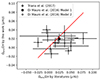 |
Fig. 8. Comparison of envelope rotation rates between this work and literature. We collected the 13 red giant stars by Triana et al. (2017) and KIC 4448777 by Di Mauro et al. (2016). The red line shows the 1:1 relation. |
4. Discussion
4.1. Core rotation rate Ωcore
Figure 9 displays the measurements of the core and the envelope rotation rates of 2006 stars in our sample. We show both core and envelope rotations as a function of mixed mode density, stellar mass, and radius.
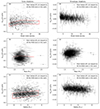 |
Fig. 9. Results of the core and the envelope rotation rates of our sample. The left column (panels a, b, c) shows the core rotation rates as a function of mixed mode density, stellar mass, and radius. The right column (panels d, e, f) is the counterpart of envelope rotations. The open points are the stars identified below the ΔΠ1–Δν sequence in Fig. 14. The dashed lines in panel (a) circle the over-density ridge. |
In panel (a), we show the core rotation rates as a function of mixed mode density, which is defined as  and has been shown as a good proxy of stellar evolution (Gehan et al. 2018). We find that the points show a bimodal distribution, formed by a narrow over-density ridge and an extended background. The over-density ridge is located at approximately Ωg/2π ∼ 0.6 μHz with width ∼ ± 0.1 μHz (circled by the dashed red lines in panel (a) of Fig. 9). We visually find that the over-density ridge might slightly increase with evolution while the extended background remains consistent with evolution. Overall speaking, no clear correlation between core rotation and evolution is apparent. We give a further discussion of the over-density ridge in Section 4.2.
In panel (b) of Fig. 9, we present the core rotation rates as a function of stellar mass which is determined by the scaling relation proposed by Yu et al. (2018). Many studies have shown that main sequence stars rotate nearly rigidly and their rotation rates increase rapidly with stellar mass, especially from ∼1.0 M⊙ to ∼1.4 M⊙, which is the transition range from stars with convective envelopes to stars with radiative envelope (Royer et al. 2007; McQuillan et al. 2014; Li et al. 2020b). However, in red giant stars, we find no obvious correlation between core rotation rate and stellar mass. This suggests that the redistribution of angular momentum transport after the main sequence is sufficiently efficient to erase the previous rotation information. Eggenberger et al. (2022b) showed that the calibrated version of the Tayler instability predicts no correlation of the core rotation rates with stellar mass for RGB stars, consistent with our observations. The over-density ridge mentioned in panel (a) is more significant in panel (b). We see a clear gap at Ωcore ≈ 0.88 μHz (marked by the dashed red line). This gap is also discovered by Hatt et al. (in prep.).
Panel (c) presents the core rotation rate as a function of stellar radius. We still observe the over-density ridge for core rotation rates (circled by the dashed red lines). The over-density ridge exhibits a slightly increasing trend between the core rotation rate and radius, indicating that as the stellar radius expands, the core experiences a slight acceleration in its rotation since the core is contracting.
In Fig. 9, the open circles refer to the stars whose ΔΠ1 are smaller than expected (Deheuvels et al. 2022; Rui & Fuller 2021). These stars might undergo a mass transfer or merger process, but do not show any special distribution of core rotation rates. We will provide more information in Section 4.5.
4.2. The over-density ridge of Ωcore
To further characterise the over-density ridge of the core rotations in panel (a) of Fig. 9, we divided the mixed mode density 𝒩 into several bins (with 𝒩∈ [3, 5], [5, 7], [7, 9], [9, 11], [11, 13] ), and fitted a two-Gaussian probability function to the core rotations in each bin. The two-Gaussian probability function is constructed as
formed by the sum of two Gaussian distributions. The first term on the right-hand side represents the over-density ridge with a mean of μ1 and a standard deviation of σ1, while the second term shows the extended background with a mean of μ2 and a standard deviation of σ2. The parameter K represents the ratio of the height of the two Gaussian distributions. Since the over-density ridge exhibits higher distribution density, we require K to be smaller than 1 but larger than 0. Additionally, the over-density ridge also shows a smaller scatter than the background, so we set 0 < σ1 < σ2. The normalisation parameter A is used to ensure that the integration of the probability function equals one.
To search for the best-fitting of  , we maximise the likelihood function defined as
The likelihood function L represents the probability of obtaining the observed core rotation distribution  given the parameter set {μ1,σ1,μ2,σ2,K}. It is calculated as the product of probabilities at each core rotation rate
  , where i means the ith core rotation value. To maximise this likelihood, we also used a Markov Chain Monte Carlo (MCMC) code implemented in the Python package emcee (Foreman-Mackey et al. 2013). Non-informative priors were used for the parameters.
Figure 10 presents the best-fitting two-Gaussian distributions in each bin of mixed mode density 𝒩. We find that the two-Gaussian distributions effectively reproduce the observed histograms of core rotation rates when 𝒩 ranges from 3 to 11 (panels (1) to (4)), as indicated by the well-constrained parameters obtained from the MCMC fit. However, for 𝒩 values from 11 to 13 (panel (5)), we face challenges in obtaining accurate constraints for μ2, σ2, and K. Particularly, the MCMC chains suggest that K converges to zero, suggesting that a single Gaussian distribution adequately reproduces the observed histogram.
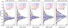 |
Fig. 10. Two-Gaussian fit of the core rotation rate distributions in each bin of mixed mode density 𝒩. The grey histograms are the observed distributions of core rotation rates. The blue lines correspond to the first term on the right-hand side of Eq. (21), characterised by μ1 and σ1, which represent the over-density ridge. The blue horizontal lines and shaded areas illustrate the means and 1-σ regions of the over-density ridge in each bin. The red lines depict the second term on the right-hand side of Eq. (21), characterised by μ2 and σ2, representing the extended background. The black lines indicate the sum of the two Gaussian distributions, which provide a good reproduction of the observed histogram. |
To further confirm whether the two-Gaussian model (Eq. (21), hereafter named model M2) is statistically more significant than a single-Gaussian model (model M1) to represent the distribution of core rotation rates, we computed the odd ratio, that can be reduced to the Bayes factor (e.g. Deheuvels et al. 2015) defined as
where P(D|Mi) is the global likelihood (or evidence) of model Mi, that is the probability for model Mi to produce the data set D. It is obtained by marginalisation, that is the integration of the likelihood over the whole parameter space (see discussion for example in Benomar et al. 2009). To compute the evidences of models M1 and M2, we use a parallel tempering MCMC code we developed in the past (Deheuvels et al. 2015). We then computed the logarithmic Bayes factor lnB21 to test the ability for model M2 to better represent the distribution of rotation than model M1. For the four distributions obtained with 𝒩 < 11, we get lnB21 ranging between 29 and 13. According to Jeffreys’ scale (Jeffreys 1961), values above 5 are decisive evidences for model M2 against model M1. However, for the last distribution (11 < 𝒩 < 13), we get lnB21 ≈ −0.5, that confirms that a single Gaussian law is enough to model this distribution. Therefore, we confirm that the over-density ridge is statistically significant up to 𝒩 = 11.
The mean value μ2 and the standard deviation σ2 of the extended background exhibit consistency across the range of 𝒩 values from 3 to 11, indicating no significant variations in the distributions of the extended background. On the other hand, the mean value μ1 of the over-density ridge increases from 𝒩 = 3 to 7 and remains constant thereafter. This measurement of μ1 aligns with the visual inspection of the over-density ridge depicted in panel (a) of Fig. 9.
Currently, the origin of this bimodal distribution still have to be understood. We investigated the stellar parameters of the stars within the over-density ridge, such as the seismic parameters (q, fshift, and Ωcore) or global parameters (mass, metallicity, and log g), without finding any significant correlations or trends.. As the bimodal distribution emerges when 𝒩 < 13, we speculate that the mechanism responsible for the formation of the bimodal distribution might be significant in late subgiant to young RGB stars, but gradually disppears with stellar evolution.
4.3. Envelope rotations
Panels (d) and (e) of Fig. 9 show the envelope rotations as a function of mixed mode density and stellar mass. Although our code reports some negative envelope rotation rates of some stars, the envelope rotations of the majority are consistent with zero within 3σ. We detect significant (above a 3-σ detection threshold) positive envelope rotation rates in 243 stars. We also measure negative rotation rates above a 3-σ detection threshold in only 33 stars. The reason for the negative values is twofold. First, most of the stars in our sample have envelope rotation rates that are distributed around 0.025 μHz (corresponding to 463 days), which is close to the detection limit of 1400-day asteroseismic data by Kepler. Second, p-dominated mixed modes usually have wider linewidths and larger frequency uncertainties, which results in fewer constraints on envelope rotation compared to g-dominated modes on core rotation. Consequently, a few negative envelope rotation results might be reported by our code. In Fig. 11, we show the stretched échelle diagram of KIC 10817031, which exhibits the smallest negative value of envelope rotation (Ωenv/(2π) = − 0.102 ± 0.026 μHz) among our sample. We attribute the negative envelope rotation in this star to the limited number of splittings observed in p-dominated modes, which do not provide sufficient constraints on the envelope rotation rate.
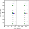 |
Fig. 11. Stretched échelle diagram of KIC 10817031, which shows a negative envelope rotation rate due to the limited number of rotational splittings. |
In panel (d), a significant decreasing trend is observed between envelope rotation and mixed mode density. This can be attributed to the expansion of the stellar envelope, which leads to a deceleration of the envelope rotation (this interpretation is further supported by panel (f), which confirms that the envelope rotation rate shows a decreasing trend as a function of the stellar radius). At the beginning of the red giant phase (with a mixed mode density around 4), the envelope rotation rates are distributed between 0 and 0.05 μHz, corresponding to rotation periods of approximately 460 days. As stars expand, the envelope rotation rates decrease and eventually distribute around 0 μHz. This indicates that current asteroseismic data provide limited constraints on envelope rotation rates due to the expansion of stars. In panel (e), the relation between envelope rotation rates and stellar masses is examined, yet no correlation is found between them.
In Fig.12, we plot the relation between envelope rotation Ωenv and stellar radius R for the 243 RGB stars with significant measurements. Additionally, we include data from other studies, including six young post-main sequence stars from Deheuvels et al. (2014), and two young subgiants from Deheuvels et al. (2020). In a simplified scenario, the envelope rotation is expected to scale as R−2. We find that this relation holds for the RGB stars in our sample. The best-fitting relation is given by

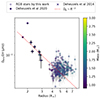 |
Fig. 12. Envelope rotation rate as a function of stellar radius. We include 243 RGB stars by this work whose envelope rotation rates are outside three sigma deviation from zero, six young RGB stars by Deheuvels et al. (2014), and two young RGB stars by Deheuvels et al. (2020). The red dotted line shows the best fitting results assuming the envelope rotation decreases with R−2, which is Ωp/2π = 0.97/R2. |
plotted as the red dotted line in Fig. 12. Notably, the young RGB stars with R < 3.5 R⊙ exhibit a smaller scatter around this relation. In contrast, the RGB stars from our study with 4 R⊙ < R < 8 R⊙ show a larger spread in their envelope rotation rates. There may be several reasons for the increased spread of envelope rotation rates during the transition from subgiants to young red giants. One reason is the bias of the data; currently, there are only eight subgiant samples (Deheuvels et al. 2014, 2020), which is far from sufficient to delineate the statistical characteristics of surface rotations in subgiants. Another reason is that as the stars expand, certain physical processes, such as the engulfment of planets (Tayar et al. 2022; Kunitomo et al. 2011; Hon et al. 2023) or the tidal effects of nearby companions (e.g. Ahuir et al. 2021), become more significant. These can all potentially impact the envelope rotation rates.
The stars which might undergo a mass transfer or merger process (open circles in Fig. 9) still do not show any special envelope rotation rates. This implies that the mass transfer or merger process might not lead to an obvious change in surface rotation rates.
4.4. Differential rotation
Our analysis of core and envelope rotation rates in RGB stars allows us to examine the core-to-surface differential rotations, specifically the ratio between the core and envelope rotation rates, denoted as Ωcore/Ωenv. To ensure reliable measurements and avoid issues associated with near-zero or negative estimates of Ωenv, we only consider the 243 stars with a significant measurements in the envelop (the same stars as in Fig. 12). It is important to note that this selection leads to a bias towards low values of the reported ratio distribution, as many stars with near-zero envelope rotations are discarded.
In Fig. 13, we examine the relation between the ratio of core-to-envelope rotation rates, Ωcore/Ωenv, and the mixed mode density 𝒩. This analysis provides insights into how differential rotation evolves with stellar evolution. In addition to the 243 red-giant-branch (RGB) stars analysed in this work, we also include six young red giants studied by Deheuvels et al. (2014), two young subgiants exhibiting solid-body rotation profiles reported by Deheuvels et al. (2020), and 17 young red giants by Li, Yaguang et al. (in prep.). We find that as stars evolve, the ratio Ωcore/Ωenv increases significantly from around 1 at 𝒩 ∼ 0.1 to approximately 20 at 𝒩 ∼ 1 (Deheuvels et al. 2014, 2020). Our sample consists of more evolved stars, with 𝒩 ranging from approximately 3 to 20. The core-to-envelope rotation ratios of our stars fall within the range of around 10–50, exhibiting a larger spread compared to the young stars. We speculate that this increased spread may be caused by the increased spread of envelope rotation rates (we refer to the discussion in Sect. 4.3). Moreover, based on the measurements of the seven helium-burning stars reported by Deheuvels et al. (2015), Once the stars enter the helium-burning phase, their differential rotations become mild, and the core-to-envelope rotation ratios are typically around two or three.
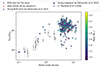 |
Fig. 13. Ratio between core and envelope rotation rates of evolved stars, including 243 RGB stars by this work whose envelope rotation rates are outside three sigma deviation from zero. We also show the six young RGB stars by Deheuvels et al. (2014) and seven helium-burning stars by Deheuvels et al. (2015). |
It is intriguing to note that six stars in our sample exhibit extremely mild differential rotations, with Ωcore/Ωenv < 2. They are KIC 4279009, 6956834, 7257241, 7630743, 8352953, and 11294612. Among them, KIC 7630743 is the one that has the smallest Ωcore/Ωenv. Our measurements indicate that Ωcore/2π = 0.065 ± 0.007 μHz and Ωenv/2π = 0.063 ± 0.012 μHz, hence the ratio Ωcore/Ωenv is only 1.04 ± 0.24. KIC 7630743 thus becomes the first red giant that is found to have a nearly uniform rotation. We show the rotational splittings of KIC 7630743 in Fig. D.1.
We find that these rigidly rotating RGB stars exhibit typical envelope rotation rates. Their rigid rotation profiles are attributed to the extremely slow rotation rates of their cores. One hypothesis is that their progenitors, during the main sequence phase, were extremely slow rotators within binary systems, as discovered by Li et al. (2020a). These stars exhibit γ Doradus-type pulsations, and their near-core rotation rates are on the order of hundreds of days. Fuller (2021) proposed the concept of “inverse tides” to explain this slow rotation: tidal interaction with unstable pulsation modes can force the spins of the stars away from synchronicity. As these stars evolve into the RGB phase, they may retain their slowly rotating cores, resulting in rigid rotation profiles.
4.5. Stars below ΔΠ1–Δν degenerate sequence and their q values
In this section, besides the rotation part, we report the result of the ΔΠ1–Δν sequence. The ΔΠ1–Δν sequence was noticed by several previous studies (e.g. Stello et al. 2013; Mosser et al. 2014; Vrard et al. 2016). Deheuvels et al. (2022) demonstrated that red giants join the ΔΠ1–Δν sequence when electron degeneracy becomes strong in the cores. The stars above the sequence might be because their cores have not yet reached electron degeneracy, or their masses are too large to reach the degeneracy. For those below the sequence, a process of mass transfer or a stellar merger was proposed to address the core-to-envelope inconsistency (see Deheuvels et al. 2022; Rui & Fuller 2021). Strong central magnetic fields can also generate smaller apparent ΔΠ1 (Loi 2020; Li et al. 2022a; Bugnet 2022; Deheuvels et al. 2023), but we have removed them from our sample. Here we present our measurements of the degenerate sequence in Fig. 14. Our results successfully reproduce the sequence, and we also observe the expected mass gradient, with higher-mass stars tending to be located at the lower boundary of the sequence. We show the mass-transfer or merger remnants by Deheuvels et al. (2022) and Rui & Fuller (2021), and we also identify more stars that are located below the sequence (marked by the red dots). The criterion is that the ΔΠ1 value of a star is six seconds smaller than the ΔΠ1–Δν linear fit.
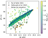 |
Fig. 14. ΔΠ1–Δν degenerate sequence, colour-coded by the scaling-relation mass by Yu et al. (2018). The plus symbol (‘+’) marks the stars reported by Rui & Fuller (2021), and the cross symbol (‘×’) are reported by Deheuvels et al. (2022). The red dots mark the stars that are located six seconds below the sequence (dotted line) by this work. |
In order to test further the scenario that these stars have undergone a mass transfer process, we examined whether they exhibit any unusual parameter distributions. These stars are highlighted in Fig. 9 as empty dots. They show normal core and envelope rotation rates. Interestingly, as shown in panel (b) in Fig. 9, the stars below the ΔΠ1–Δν sequence all show relatively large masses (≳1.5 M⊙), which is another evidence that they underwent a process of mass transfer or merger, but these stars still show normal core rotation rates. We also examined their other parameters (q, εg, fshift) and found no significant deviations, except for q.
The coupling factor q stands for the coupling strength between p- and g-mode cavities and provides structure information of the evanescent region between the two cavities for low-luminosity red giants (Takata 2016; Mosser et al. 2017b; Hekker et al. 2018; Pinçon et al. 2020; Jiang et al. 2020). In our study, we assume that the q value is the same for all modes, although Jiang et al. (2020) has shown a frequency dependence. We present the measurement of the coupling factor q in Fig. 15. We find that the value q distributes between ∼0.2 and ∼0.1 and decreases with descending Δν, forming a q-Δν linear relation (Mosser et al. 2017b). The linear relation is caused by the progressive migration of the evanescent region from the radiative to the convective zones within the star (Pinçon et al. 2020). In Fig. 15, we find that most of the stars under the ΔΠ1-Δν sequence show smaller values of q. This is because these stars should have older cores with smaller q, while mass transfer from their companions leads to an increase in mean density, resulting in a larger Δν. As a result, they are located below the q-Δν sequence.
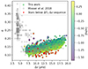 |
Fig. 15. Coupling factor, q, as a function of Δν, colour-coded by metallicity. The grey circles are reported by Mosser et al. (2018). Our results are consistent with the results of the RGB stars by Mosser et al. (2018), while plenty of helium-burning stars show much larger q and much smaller Δν. A clear metallicity gradient is seen in the figure. The stars which might undergo mass transfer processes tend to have smaller q value. |
A large spread of the correlation between q and Δν is seen, which is caused by different metallicity and stellar mass. The clear metallicity gradient visible in Fig. 15 indicates that low-metallicity stars tend to exhibit larger q values. Additionally, in Fig. 16, we can see a weak correlation with stellar mass, although not as pronounced as the effect of metallicity. Stars with smaller masses tend to display larger values of q. Furthermore, we also notice that the stars below the ΔΠ1-Δν sequence show larger stellar mass (M ≳ 1.5 M⊙, also shown later in panels (b) and (e) of Fig. 9), consistent with the hypothesis that they gain extra material from companion stars. The dependences between q and metallicity (and mass) have been reported by Kuszlewicz et al. (2023). Our larger sample further confirms their discovery.
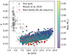 |
Fig. 16. Same as Fig. 15 but colour-coded by stellar mass. The gradient caused by mass is weaker but is still visible. |
5. Conclusions
In this work, we report the largest sample of Kepler RGB stars with clearly identified and analysed mixed-mode patterns. Overall, we measured mixed-mode properties for 2495 RGB stars. Among them, 2006 stars show rotational splittings, including 800 stars showing doublets and 1206 stars showing triplets. There are also 489 stars that show only m = 0 modes.
One of our main goals was to reliably measure envelope rotation rate for a large sample of RGB stars. In this work, we argued that the methods that were previously applied to infer the internal rotation of red giants (rotation inversions, linear regression of the relation between the rotational splitting and the ζ parameter) do not account for near-degeneracy effects (NDE, Deheuvels et al. 2017). We showed that this leads to biases in the estimates of envelope rotation rates, which become stronger as stars ascend the RGB. We proposed an alternate approach to fitting asymptotic expressions of mixed modes to the observations without resorting to the ζ function and we showed that it properly treats NDE. This new approach provides more reliable measurements of the envelope rotation rate.
Using this new approach, we measured the following mixed-mode parameters for each star: period spacing, ΔΠ1, coupling factor, q, g-mode offset term, εg, frequency correction of pure dipole p mode, fshift (linked to the small separation, δν01), mean core rotation rate, Ωcore, and the mean envelope rotation rate, Ωenv. Asymptotic relations were also fitted to l = 0 and 2 pressure mode frequencies. The envelope rotation rate, in particular, is measured in such a large sample for the first time.
The core rotation sample we reported is twice as large as that in previous studies, allowing us to investigate the detailed structure of core rotation as it evolves. We confirm previous findings that there is no obvious correlation between the core rotation rates and evolution. However, we uncovered the existence of an over-density ridge, or bimodal distribution, for core rotation rates as a function of the evolution along the RGB. Indeed, a population of red giants shows core rotation rates that are narrowly distributed around about 0.6 μHz, while other red giants show larger scatter. The central peak of this newly identified distribution slightly increases with evolution, which suggests that the cores of this sub-population of red giants might be spinning up, in contrast with other red giants. This implies that there might be two populations of RGB stars whose cores undergo different rotational evolution. Currently, we cannot provide any theoretical explanation for the formation of the over-density ridge. However, it could provide precious information about the way angular momentum is transported in the subgiant and RGB phases.
We increased the sample of the envelope rotation rate measurements by two orders of magnitude. We find that there is a clear spin-down of the envelope rotation rates as a function of stellar evolution and radius due to the expansion of stars. For more evolved red giants, the envelope rotation rates of most stars are too slow to be significantly measured, even with the longest Kepler data sets. We obtain 243 stars whose envelope rotation rates are significantly larger than zero, among a total of 2006 stars for which the internal rotation could be probed. The core-to-envelope rotation ratios of these stars are measured. We find that the ratios distribute around ∼20. This is to be understood as the lower-end of the distribution because we ignore a lot of stars whose envelope rotation rates are close to zero. The core-to-envelope ratios Ωcore/Ωenv show a larger spread compared to the stars in the subgiant phase (Deheuvels et al. 2014, 2020), suggesting various processes of angular momentum transport at the transition between subgiants and red giants. Our observations will be important to measure the efficiency of angular momentum transport along the RGB since for this purpose a core-envelope rotation ratio is needed (Eggenberger et al. 2019). Interestingly, we also find several RGB stars showing extremely mild radial differential rotations (with Ωcore/Ωenv < 2), which had not been reported before. We find that the envelope rotation rates of these stars are quite typical, but their cores are rotating much slower than those of the bulk of Kepler red giants. These stars might be the evolved counterparts of γ Doradus-type stars that exhibit extremely slow near-core rotation during the main sequence (Li et al. 2020a), which has been interpreted as a potential consequence of tidal interactions (Fuller 2021).
As a by-product of this work, we also find a group of new stars which show smaller ΔΠ1 compared to the ΔΠ1–Δν degenerate sequence. We confirm the previous discovery by Kuszlewicz et al. (2023) that the stars below the ΔΠ1–Δν degenerate sequence show smaller q values, which is proof that stars might have undergone a process of mass transfer or binary merger. We also discover that many stars show larger εg, which might be a new clue for their central magnetic fields (Li et al. 2022a). We are currently investigating this possible interpretation.
Data availability
The electronic tables containing all the asteroseismic parameters and mode identifications are available at the Zenodo link https://zenodo.org/records/13207485
Acknowledgments
The authors acknowledge support from the project BEAMING ANR-18-CE31-0001 of the French National Research Agency (ANR) and from the Centre National d’Etudes Spatiales (CNES). The research leading to these results has received funding from the KU Leuven Research Council (grant C16/18/005: PARADISE). GL acknowledges the Research Foundation Flanders (FWO) Grant for a long stay abroad (grant V422323N) and the Dick Hunstead Fund for Astrophysics for his 2-month stay at the University of Sydney. GL acknowledge the travel support from the National Natural Science Foundation of China (NSFC) through the grant 12273002. GL thanks Dr. Yaguang Li for generously sharing their data. GL also thanks Professor Dennis Stello and Emily Hatt for the private discussion about the over-density ridge. This paper includes data collected by the Kepler mission and obtained from the MAST data archive at the Space Telescope Science Institute (STScI). Funding for the Kepler mission is provided by the NASA Science Mission Directorate. STScI is operated by the Association of Universities for Research in Astronomy, Inc., under NASA contract NAS 5–26555.
References
- Aerts, C., Mathis, S., & Rogers, T. M. 2019, ARA&A, 57, 35 [Google Scholar]
- Ahuir, J., Mathis, S., & Amard, L. 2021, A&A, 651, A3 [NASA ADS] [CrossRef] [EDP Sciences] [Google Scholar]
- Anderson, E. R., Duvall, T. L. Jr., & Jefferies, S. M. 1990, ApJ, 364, 699 [NASA ADS] [CrossRef] [Google Scholar]
- Ballot, J., Appourchaux, T., Toutain, T., & Guittet, M. 2008, A&A, 486, 867 [NASA ADS] [CrossRef] [EDP Sciences] [Google Scholar]
- Barrère, P., Guilet, J., Raynaud, R., & Reboul-Salze, A. 2023, MNRAS, 526, L88 [CrossRef] [Google Scholar]
- Beck, P. G., Montalban, J., Kallinger, T., et al. 2012, Nature, 481, 55 [Google Scholar]
- Bedding, T. R. 2014, in Asteroseismology, eds. P. L. Pallé, & C. Esteban (Cambridge, UK: Cambridge University Press), 60 [CrossRef] [Google Scholar]
- Bedding, T. R., Huber, D., Stello, D., et al. 2010, ApJ, 713, L176 [Google Scholar]
- Bedding, T. R., Mosser, B., Huber, D., et al. 2011, Nature, 471, 608 [Google Scholar]
- Belkacem, K., Marques, J. P., Goupil, M. J., et al. 2015, A&A, 579, A30 [NASA ADS] [CrossRef] [EDP Sciences] [Google Scholar]
- Benomar, O., Appourchaux, T., & Baudin, F. 2009, A&A, 506, 15 [NASA ADS] [CrossRef] [EDP Sciences] [Google Scholar]
- Benomar, O., Takata, M., Shibahashi, H., Ceillier, T., & García, R. A. 2015, MNRAS, 452, 2654 [Google Scholar]
- Borucki, W. J., Koch, D., Basri, G., et al. 2010, Science, 327, 977 [Google Scholar]
- Bugnet, L. 2022, A&A, 667, A68 [NASA ADS] [CrossRef] [EDP Sciences] [Google Scholar]
- Bugnet, L., Prat, V., Mathis, S., et al. 2021, A&A, 650, A53 [NASA ADS] [CrossRef] [EDP Sciences] [Google Scholar]
- Cantiello, M., Mankovich, C., Bildsten, L., Christensen-Dalsgaard, J., & Paxton, B. 2014, ApJ, 788, 93 [Google Scholar]
- Ceillier, T., Eggenberger, P., García, R. A., & Mathis, S. 2013, A&A, 555, A54 [NASA ADS] [CrossRef] [EDP Sciences] [Google Scholar]
- Chontos, A., Sayeed, M., & Huber, D. 2021, Posters from the TESS Science Conference II (TSC2), 189 [Google Scholar]
- Christensen-Dalsgaard, J. 2008, Ap&SS, 316, 113 [Google Scholar]
- Cunha, M. S., Stello, D., Avelino, P. P., Christensen-Dalsgaard, J., & Townsend, R. H. D. 2015, ApJ, 805, 127 [NASA ADS] [CrossRef] [Google Scholar]
- Deheuvels, S., García, R. A., Chaplin, W. J., et al. 2012, ApJ, 756, 19 [Google Scholar]
- Deheuvels, S., Doğan, G., Goupil, M. J., et al. 2014, A&A, 564, A27 [NASA ADS] [CrossRef] [EDP Sciences] [Google Scholar]
- Deheuvels, S., Ballot, J., Beck, P. G., et al. 2015, A&A, 580, A96 [NASA ADS] [CrossRef] [EDP Sciences] [Google Scholar]
- Deheuvels, S., Ouazzani, R. M., & Basu, S. 2017, A&A, 605, A75 [NASA ADS] [CrossRef] [EDP Sciences] [Google Scholar]
- Deheuvels, S., Ballot, J., Eggenberger, P., et al. 2020, A&A, 641, A117 [EDP Sciences] [Google Scholar]
- Deheuvels, S., Ballot, J., Gehan, C., & Mosser, B. 2022, A&A, 659, A106 [NASA ADS] [CrossRef] [EDP Sciences] [Google Scholar]
- Deheuvels, S., Li, G., Ballot, J., & Lignières, F. 2023, A&A, 670, L16 [NASA ADS] [CrossRef] [EDP Sciences] [Google Scholar]
- Di Mauro, M. P., Ventura, R., Cardini, D., et al. 2016, ApJ, 817, 65 [NASA ADS] [CrossRef] [Google Scholar]
- Eggenberger, P. 2015, in New Windows on Massive Stars, eds. G. Meynet, C. Georgy, J. Groh, & P. Stee, IAU Symp., 307, 165 [NASA ADS] [Google Scholar]
- Eggenberger, P., Montalbán, J., & Miglio, A. 2012, A&A, 544, L4 [NASA ADS] [CrossRef] [EDP Sciences] [Google Scholar]
- Eggenberger, P., Deheuvels, S., Miglio, A., et al. 2019, A&A, 621, A66 [NASA ADS] [CrossRef] [EDP Sciences] [Google Scholar]
- Eggenberger, P., Buldgen, G., Salmon, S. J. A. J., et al. 2022a, Nat. Astron., 6, 788 [NASA ADS] [CrossRef] [Google Scholar]
- Eggenberger, P., Moyano, F. D., & den Hartogh, J. W. 2022b, A&A, 664, L16 [NASA ADS] [CrossRef] [EDP Sciences] [Google Scholar]
- Foreman-Mackey, D., Hogg, D. W., Lang, D., & Goodman, J. 2013, PASP, 125, 306 [Google Scholar]
- Fuller, J. 2021, MNRAS, 501, 483 [Google Scholar]
- Fuller, J., Lecoanet, D., Cantiello, M., & Brown, B. 2014, ApJ, 796, 17 [Google Scholar]
- Fuller, J., Cantiello, M., Stello, D., Garcia, R. A., & Bildsten, L. 2015, Science, 350, 423 [Google Scholar]
- Fuller, J., Piro, A. L., & Jermyn, A. S. 2019, MNRAS, 485, 3661 [NASA ADS] [Google Scholar]
- Gehan, C., Mosser, B., Michel, E., Samadi, R., & Kallinger, T. 2018, A&A, 616, A24 [NASA ADS] [CrossRef] [EDP Sciences] [Google Scholar]
- Gehan, C., Mosser, B., Michel, E., & Cunha, M. S. 2021, A&A, 645, A124 [NASA ADS] [CrossRef] [EDP Sciences] [Google Scholar]
- Gizon, L., & Solanki, S. K. 2003, ApJ, 589, 1009 [Google Scholar]
- Gomes, P., & Lopes, I. 2020, MNRAS, 496, 620 [NASA ADS] [CrossRef] [Google Scholar]
- Gough, D. O. 2015, Space Sci. Rev., 196, 15 [NASA ADS] [CrossRef] [Google Scholar]
- Goupil, M. J., Mosser, B., Marques, J. P., et al. 2013, A&A, 549, A75 [NASA ADS] [CrossRef] [EDP Sciences] [Google Scholar]
- Grosjean, M., Dupret, M. A., Belkacem, K., et al. 2014, A&A, 572, A11 [CrossRef] [EDP Sciences] [Google Scholar]
- Hekker, S., Elsworth, Y., & Angelou, G. C. 2018, A&A, 610, A80 [NASA ADS] [CrossRef] [EDP Sciences] [Google Scholar]
- Hon, M., Huber, D., Rui, N. Z., et al. 2023, Nature, 618, 917 [CrossRef] [Google Scholar]
- Huber, D., Stello, D., Bedding, T. R., et al. 2009, Commun. Asteroseismol., 160, 74 [Google Scholar]
- Jeffreys, H. 1961, The Theory of Probability (Oxford: Oxford Univ. Press) [Google Scholar]
- Jiang, C., Cunha, M., Christensen-Dalsgaard, J., & Zhang, Q. 2020, MNRAS, 495, 621 [Google Scholar]
- Jouve, L., Gastine, T., & Lignières, F. 2015, A&A, 575, A106 [NASA ADS] [CrossRef] [EDP Sciences] [Google Scholar]
- Karoff, C. 2008, PhD Thesis, Aarhus University, Denmark [Google Scholar]
- Kissin, Y., & Thompson, C. 2015, ApJ, 808, 35 [NASA ADS] [CrossRef] [Google Scholar]
- Kunitomo, M., Ikoma, M., Sato, B., Katsuta, Y., & Ida, S. 2011, ApJ, 737, 66 [Google Scholar]
- Kuszlewicz, J. S., Hon, M., & Huber, D. 2023, ApJ, 954, 152 [NASA ADS] [CrossRef] [Google Scholar]
- Li, G., Guo, Z., Fuller, J., et al. 2020a, MNRAS, 497, 4363 [Google Scholar]
- Li, G., Van Reeth, T., Bedding, T. R., et al. 2020b, MNRAS, 491, 3586 [Google Scholar]
- Li, G., Deheuvels, S., Ballot, J., & Lignières, F. 2022a, Nature, 610, 43 [NASA ADS] [CrossRef] [Google Scholar]
- Li, Y., Bedding, T. R., Murphy, S. J., et al. 2022b, Nat. Astron., 6, 673 [NASA ADS] [CrossRef] [Google Scholar]
- Li, G., Deheuvels, S., Li, T., Ballot, J., & Lignières, F. 2023, A&A, 680, A26 [NASA ADS] [CrossRef] [EDP Sciences] [Google Scholar]
- Lindsay, C. J., Ong, J. M. J., & Basu, S. 2022, ApJ, 931, 116 [CrossRef] [Google Scholar]
- Loi, S. T. 2020, MNRAS, 496, 3829 [Google Scholar]
- Loi, S. T. 2021, MNRAS, 504, 3711 [NASA ADS] [CrossRef] [Google Scholar]
- Loi, S. T., & Papaloizou, J. C. B. 2017, MNRAS, 467, 3212 [NASA ADS] [Google Scholar]
- Loi, S. T., & Papaloizou, J. C. B. 2018, MNRAS, 477, 5338 [Google Scholar]
- Lund, M. N., Silva Aguirre, V., Davies, G. R., et al. 2017, ApJ, 835, 172 [Google Scholar]
- Maeder, A. 2009, Physics, Formation and Evolution of Rotating Stars (Berlin, Heidelberg: Springer) [Google Scholar]
- Maeder, A., & Meynet, G. 2014, ApJ, 793, 123 [Google Scholar]
- Marques, J. P., Goupil, M. J., Lebreton, Y., et al. 2013, A&A, 549, A74 [NASA ADS] [CrossRef] [EDP Sciences] [Google Scholar]
- Mathis, S., & Bugnet, L. 2023, A&A, 676, L9 [NASA ADS] [CrossRef] [EDP Sciences] [Google Scholar]
- Mathis, S., & Zahn, J. P. 2004, A&A, 425, 229 [NASA ADS] [CrossRef] [EDP Sciences] [Google Scholar]
- Mathis, S., Prat, V., Amard, L., et al. 2018, A&A, 620, A22 [NASA ADS] [CrossRef] [EDP Sciences] [Google Scholar]
- Mathis, S., Bugnet, L., Prat, V., et al. 2021, A&A, 647, A122 [EDP Sciences] [Google Scholar]
- McQuillan, A., Mazeh, T., & Aigrain, S. 2014, ApJS, 211, 24 [Google Scholar]
- Mosser, B., Belkacem, K., Goupil, M. J., et al. 2011, A&A, 525, L9 [CrossRef] [EDP Sciences] [Google Scholar]
- Mosser, B., Goupil, M. J., Belkacem, K., et al. 2012a, A&A, 548, A10 [NASA ADS] [CrossRef] [EDP Sciences] [Google Scholar]
- Mosser, B., Goupil, M. J., Belkacem, K., et al. 2012b, A&A, 540, A143 [NASA ADS] [CrossRef] [EDP Sciences] [Google Scholar]
- Mosser, B., Benomar, O., Belkacem, K., et al. 2014, A&A, 572, L5 [NASA ADS] [CrossRef] [EDP Sciences] [Google Scholar]
- Mosser, B., Vrard, M., Belkacem, K., Deheuvels, S., & Goupil, M. J. 2015, A&A, 584, A50 [NASA ADS] [CrossRef] [EDP Sciences] [Google Scholar]
- Mosser, B., Belkacem, K., Pinçon, C., et al. 2017a, A&A, 598, A62 [NASA ADS] [CrossRef] [EDP Sciences] [Google Scholar]
- Mosser, B., Pinçon, C., Belkacem, K., Takata, M., & Vrard, M. 2017b, A&A, 600, A1 [NASA ADS] [CrossRef] [EDP Sciences] [Google Scholar]
- Mosser, B., Gehan, C., Belkacem, K., et al. 2018, A&A, 618, A109 [NASA ADS] [CrossRef] [EDP Sciences] [Google Scholar]
- Moyano, F. D., Eggenberger, P., Salmon, S. J. A. J., Mombarg, J. S. G., & Ekström, S. 2023, A&A, 677, A6 [NASA ADS] [CrossRef] [EDP Sciences] [Google Scholar]
- Nielsen, M. B., Schunker, H., Gizon, L., & Ball, W. H. 2015, A&A, 582, A10 [NASA ADS] [CrossRef] [EDP Sciences] [Google Scholar]
- Ong, J. M. J., & Gehan, C. 2023, ApJ, 946, 92 [CrossRef] [Google Scholar]
- Ong, J. M. J., Bugnet, L., & Basu, S. 2022, ApJ, 940, 18 [NASA ADS] [CrossRef] [Google Scholar]
- Ouazzani, R. M., Marques, J. P., Goupil, M. J., et al. 2019, A&A, 626, A121 [NASA ADS] [CrossRef] [EDP Sciences] [Google Scholar]
- Paxton, B., Bildsten, L., Dotter, A., et al. 2011, ApJS, 192, 3 [Google Scholar]
- Petitdemange, L., Marcotte, F., & Gissinger, C. 2023, Science, 379, 300 [NASA ADS] [CrossRef] [Google Scholar]
- Petitdemange, L., Marcotte, F., Gissinger, C., & Daniel, F. 2024, A&A, 681, A75 [NASA ADS] [CrossRef] [EDP Sciences] [Google Scholar]
- Pinçon, C., Belkacem, K., & Goupil, M. J. 2016, A&A, 588, A122 [NASA ADS] [CrossRef] [EDP Sciences] [Google Scholar]
- Pinçon, C., Goupil, M. J., & Belkacem, K. 2020, A&A, 634, A68 [Google Scholar]
- Royer, F., Zorec, J., & Gómez, A. E. 2007, A&A, 463, 671 [NASA ADS] [CrossRef] [EDP Sciences] [Google Scholar]
- Rüdiger, G., Gellert, M., Spada, F., & Tereshin, I. 2015, A&A, 573, A80 [NASA ADS] [CrossRef] [EDP Sciences] [Google Scholar]
- Rui, N. Z., & Fuller, J. 2021, MNRAS, 508, 1618 [NASA ADS] [CrossRef] [Google Scholar]
- Saio, H., Takata, M., Lee, U., Li, G., & Van Reeth, T. 2021, MNRAS, 502, 5856 [Google Scholar]
- Schou, J., Antia, H. M., Basu, S., et al. 1998, ApJ, 505, 390 [Google Scholar]
- Shibahashi, H. 1979, PASJ, 31, 87 [NASA ADS] [Google Scholar]
- Spada, F., Gellert, M., Arlt, R., & Deheuvels, S. 2016, A&A, 589, A23 [NASA ADS] [CrossRef] [EDP Sciences] [Google Scholar]
- Stello, D., Huber, D., Bedding, T. R., et al. 2013, ApJ, 765, L41 [CrossRef] [Google Scholar]
- Stello, D., Cantiello, M., Fuller, J., et al. 2016, Nature, 529, 364 [Google Scholar]
- Takata, M. 2016, PASJ, 68, 109 [NASA ADS] [CrossRef] [Google Scholar]
- Tassoul, M. 1980, ApJS, 43, 469 [Google Scholar]
- Tayar, J., Moyano, F. D., Soares-Furtado, M., et al. 2022, ApJ, 940, 23 [NASA ADS] [CrossRef] [Google Scholar]
- Triana, S. A., Corsaro, E., De Ridder, J., et al. 2017, A&A, 602, A62 [NASA ADS] [CrossRef] [EDP Sciences] [Google Scholar]
- Unno, W., Osaki, Y., Ando, H., Saio, H., & Shibahashi, H. 1989, Nonradial Oscillations of Stars (Tokyo: University of Tokyo Press) [Google Scholar]
- Van Reeth, T., Tkachenko, A., & Aerts, C. 2016, A&A, 593, A120 [NASA ADS] [CrossRef] [EDP Sciences] [Google Scholar]
- Vrard, M., Mosser, B., & Samadi, R. 2016, A&A, 588, A87 [CrossRef] [EDP Sciences] [Google Scholar]
- Wu, X., Li, C., de Grijs, R., & Deng, L. 2016, ApJ, 826, L14 [NASA ADS] [CrossRef] [Google Scholar]
- Yu, J., Huber, D., Bedding, T. R., et al. 2018, ApJS, 236, 42 [NASA ADS] [CrossRef] [Google Scholar]
- Zahn, J. P. 1992, A&A, 265, 115 [NASA ADS] [Google Scholar]
Appendix A: Observed splitting asymmetries in KIC 11245496
In Fig. A.1, we present the observed splitting asymmetries for KIC 11245496 as a comparison to the simulated splitting asymmetries shown in Fig. 6. We find that l = 1 modes exhibit observable splitting asymmetries similar to the l = 2 modes reported by (Deheuvels et al. 2017). Moreover, approach two successfully reproduces the observed asymmetries.
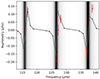 |
Fig. A.1. Observed asymmetries in l = 1 rotational multiplets in KIC 11245496. The difference to Fig. 6 is that the red dots are real observed values of asymmetries, so we can show error bars on them. |
Appendix B: The other parameters
In this section, we show the other parameters that we measure, which may not be directly related to our scientific goals but still have some interesting results.
B.1. Shift of pure l = 1 p mode fshift
In Eq. 10, we define the shift of the pure l = 1 p modes, denoted as fshift, to properly account for the locations of invisible pure p modes. Figure B.1 illustrates a correlation between fshift and Δν. As Δν decreases, fshift also decreases, ranging from approximately 0.8 to 0.4, and the spread of values becomes smaller. We observe a mass gradient in this relation, where higher-mass stars tend to exhibit smaller values of fshift.
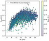 |
Fig. B.1. Shift of the pure l = 1 p modes fshift as a function of Δν. |
Therefore, we can measure the small separation δν01 defined as  . The top panel of Fig. B.2 shows δν01 of the RGB stars by this work. δν01 decreases from ∼0.2 μHz to ∼ − 0.2 μHz as Δν decreases; thus, for RGB stars, the pure l = 1 p modes are almost exactly located at the halfway between l = 0 modes. The bottom panel shows how δν0, 1 evolves from the main sequence to the red giant branch. The main sequence stars by Lund et al. (2017) show a relatively large spread of δν01, ranging from 2 μHz to 6 μHz, and their δν01 decreases with evolution and eventually converges to the RGB stars.
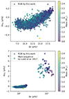 |
Fig. B.2. Small separation δ01 with Δν. Top panel: RGB stars by this work. Bottom panel: Both the RGB stars from this work and the main sequence stars from Lund et al. (2017). |
B.2. Inclination i
We obtain the stellar inclinations when fitting the Lorentzian profiles to the rotational splittings. Figure B.3 compares our results with those reported by Gehan et al. (2021). Our results show a general consistency with the inclinations by Gehan et al. (2018). The difference might come from the different mode identifications or different fitting strategies. For example, we fit the Lorentzian profiles to all the rotational splittings (as shown in Fig. C.1), whereas Gehan et al. (2021) only used g-dominated modes to fit.
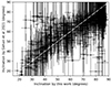 |
Fig. B.3. Comparison between the inclinations measured by this work and those reported by Gehan et al. (2021). The white dotted-dashed line stands for the 1:1 relation. |
Figure B.4 displays the distribution of stellar inclinations in our sample. The solid curve is the theoretical distribution that is proportional to sin(i), assuming isotropic orientations of stellar rotational axes. Similar to the findings of Gehan et al. (2021), we also observe a distribution that deviates from the isotropic expectation. In Fig. B.4, the number increases rapidly from i = 20° to 30° because the stars with smaller inclinations do not show any rotational splittings hence cannot be measured in our algorithm. Additionally, we identify an excess when the inclination is close to 90°, which has been referred to as ‘fit locking’ and explained by Ballot et al. (2008). Therefore, the deviation from isotropic distribution cannot prove that the directions of the stellar rotational axes are not isotropic.
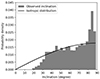 |
Fig. B.4. Distribution of stellar inclination measured by rotational splittings. |
Appendix C: Spectral fit of KIC 8636389
We show the mode identifications of azimuthal order, m, and Lorentzian fit of the mixed-mode rotational splittings of KIC 8636389 in Fig. C.1. The spectrum in Fig. C.1 is located between np = 10, l = 0 p mode and np = 10, l = 2 p mode. The best-fitting model reproduces the observed power spectrum and gives the measurements of oscillation frequencies, linewidth changes, and inclination.
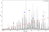 |
Fig. C.1. Fit of the whole power spectrum of KIC 8636389. We only show the sector with np = 10. The grey line is the observed power spectrum. We mark the m = −1, 0, and +1 modes by the red short line, blue circle, and green plus symbols. The horizontal red lines mark the rotational splittings. The best-fitting result is shown by the black line, from which the frequency, rotational splitting, amplitude, stellar inclination, and linewidth are derived. |
Appendix D: Rotational splittings and Lorentzian fit of KIC 7630743
In Fig. D.1 we show the detail of the observed and fitting rotational splittings of KIC 7630743. This star shows very slow rotational rates and a near-rigid radial rotation profile (see the discussion in Section 4.4).
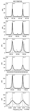 |
Fig. D.1. Rotational splittings of KIC 7630743. the grey lines show the observed power spectrum and the solid black lines show the best-fitting Lorentzian profiles. The vertical dashed lines mark the locations of m = ±1 modes. |
Appendix E: Estimating near-degeneracy-effects on dipole mixed modes in a Kepler red giant
To estimate NDEs for the chosen reference star, we followed Deheuvels et al. (2017). The authors expressed the mode displacement as a linear combination of the eigenfunctions of the unperturbed degenerate modes. They focused on l = 2 mixed modes, which have only weak coupling. Thus, they restricted their analysis to the case of two near-degenerate modes. For l = 1 modes, the coupling between the cavities is stronger, so that one p mode couples to several consecutive g modes. When NDEs play a key role, we should thus consider the general case of N degenerate modes. Contrary to what was stated by Ong et al. (2022), the development proposed in Deheuvels et al. (2017) can easily be extended to the case of N modes. The eigenfunctions of perturbed modes are then simply written as  , where ξ0, i is the eigenfunction of the ith unperturbed mode experiencing near-degeneracy. The frequencies of the near-degenerate modes are then found as the eigenvalues of the matrix M = A + R, where A is a diagonal matrix containing the square of the unperturbed frequencies of the N considered modes (
 ), and the components of matrix R are given by
where δℒR is the rotational perturbation to the oscillation operator and ⟨ ⋅ , ⋅ ⟩ is the inner product defined as  for functions ξ and η. To characterise δℒR, we needed to assume a rotation profile Ω(r). We chose a two-zone profile with a discontinuity in the evanescent zone. We then solved the eigenvalue problem to obtain the perturbed mode frequencies of the considered stellar models.
All Tables
All Figures
|
Fig. 1. Stretched échelle diagram of KIC 8636389. The x-axis is the stretched period τ module of 75.9 s. The y-axis is the oscillation frequency. The grey dots are the peaks with S/N higher than 10. The blue circles are identified as l = 1 m = 0 mixed modes. The red line and green plus are the m = −1 and m = +1 modes. The crosses show the best-fitting frequencies. |
| In the text | |
|
Fig. 2. Corner diagram of the posterior distributions of KIC 9289599 by approach two. |
| In the text | |
|
Fig. 3. Distributions of Δν (top) and mass (bottom) of our sample and the sample by Yu et al. (2018). |
| In the text | |
|
Fig. 4. Envelope rotation rates derived by approaches one and two. The colour bar indicates the intensity of NDE, calculated as the ratio between the core rotation and Δfmin, which is the smallest frequency separation between consecutive l = 1 mixed modes around νmax (see Sect. 3.1). |
| In the text | |
|
Fig. 5. Differences of the core and envelope rotation rates between approaches two and one (defined as the results from approach two minus the results from approach one). The colour bar represents the extent of the NDE (see Fig. 4 and Sect. 3.1). The horizontal dashed lines mark the location where the values are equal. The white error bars show the mean and standard deviations in each bin of Δν. |
| In the text | |
|
Fig. 6. Synthetic asymmetries in l = 1 rotational multiplets resulting from near-degeneracy effects in KIC 11245496. The red dots are the simulated asymmetries following the method by Deheuvels et al. (2017), while the grey dots and lines are the best-fitting results by approach two. The background shows the ζ values: the darker, the smaller, hence the dark fringes stand for the positions of p-dominated modes. |
| In the text | |
|
Fig. 7. Comparison between our result with previous studies. Top left: core rotation rate Ωcore. Top right: period spacing ΔΠ1. Bottom left: coupling factor q. Bottom right: g-mode phase εg. the dashed line in each panel shows the 1:1 relation, or 2:1 and 1:2 as marked. |
| In the text | |
|
Fig. 8. Comparison of envelope rotation rates between this work and literature. We collected the 13 red giant stars by Triana et al. (2017) and KIC 4448777 by Di Mauro et al. (2016). The red line shows the 1:1 relation. |
| In the text | |
|
Fig. 9. Results of the core and the envelope rotation rates of our sample. The left column (panels a, b, c) shows the core rotation rates as a function of mixed mode density, stellar mass, and radius. The right column (panels d, e, f) is the counterpart of envelope rotations. The open points are the stars identified below the ΔΠ1–Δν sequence in Fig. 14. The dashed lines in panel (a) circle the over-density ridge. |
| In the text | |
|
Fig. 10. Two-Gaussian fit of the core rotation rate distributions in each bin of mixed mode density 𝒩. The grey histograms are the observed distributions of core rotation rates. The blue lines correspond to the first term on the right-hand side of Eq. (21), characterised by μ1 and σ1, which represent the over-density ridge. The blue horizontal lines and shaded areas illustrate the means and 1-σ regions of the over-density ridge in each bin. The red lines depict the second term on the right-hand side of Eq. (21), characterised by μ2 and σ2, representing the extended background. The black lines indicate the sum of the two Gaussian distributions, which provide a good reproduction of the observed histogram. |
| In the text | |
|
Fig. 11. Stretched échelle diagram of KIC 10817031, which shows a negative envelope rotation rate due to the limited number of rotational splittings. |
| In the text | |
|
Fig. 12. Envelope rotation rate as a function of stellar radius. We include 243 RGB stars by this work whose envelope rotation rates are outside three sigma deviation from zero, six young RGB stars by Deheuvels et al. (2014), and two young RGB stars by Deheuvels et al. (2020). The red dotted line shows the best fitting results assuming the envelope rotation decreases with R−2, which is Ωp/2π = 0.97/R2. |
| In the text | |
|
Fig. 13. Ratio between core and envelope rotation rates of evolved stars, including 243 RGB stars by this work whose envelope rotation rates are outside three sigma deviation from zero. We also show the six young RGB stars by Deheuvels et al. (2014) and seven helium-burning stars by Deheuvels et al. (2015). |
| In the text | |
|
Fig. 14. ΔΠ1–Δν degenerate sequence, colour-coded by the scaling-relation mass by Yu et al. (2018). The plus symbol (‘+’) marks the stars reported by Rui & Fuller (2021), and the cross symbol (‘×’) are reported by Deheuvels et al. (2022). The red dots mark the stars that are located six seconds below the sequence (dotted line) by this work. |
| In the text | |
|
Fig. 15. Coupling factor, q, as a function of Δν, colour-coded by metallicity. The grey circles are reported by Mosser et al. (2018). Our results are consistent with the results of the RGB stars by Mosser et al. (2018), while plenty of helium-burning stars show much larger q and much smaller Δν. A clear metallicity gradient is seen in the figure. The stars which might undergo mass transfer processes tend to have smaller q value. |
| In the text | |
|
Fig. 16. Same as Fig. 15 but colour-coded by stellar mass. The gradient caused by mass is weaker but is still visible. |
| In the text | |
|
Fig. A.1. Observed asymmetries in l = 1 rotational multiplets in KIC 11245496. The difference to Fig. 6 is that the red dots are real observed values of asymmetries, so we can show error bars on them. |
| In the text | |
|
Fig. B.1. Shift of the pure l = 1 p modes fshift as a function of Δν. |
| In the text | |
|
Fig. B.2. Small separation δ01 with Δν. Top panel: RGB stars by this work. Bottom panel: Both the RGB stars from this work and the main sequence stars from Lund et al. (2017). |
| In the text | |
|
Fig. B.3. Comparison between the inclinations measured by this work and those reported by Gehan et al. (2021). The white dotted-dashed line stands for the 1:1 relation. |
| In the text | |
|
Fig. B.4. Distribution of stellar inclination measured by rotational splittings. |
| In the text | |
|
Fig. C.1. Fit of the whole power spectrum of KIC 8636389. We only show the sector with np = 10. The grey line is the observed power spectrum. We mark the m = −1, 0, and +1 modes by the red short line, blue circle, and green plus symbols. The horizontal red lines mark the rotational splittings. The best-fitting result is shown by the black line, from which the frequency, rotational splitting, amplitude, stellar inclination, and linewidth are derived. |
| In the text | |
|
Fig. D.1. Rotational splittings of KIC 7630743. the grey lines show the observed power spectrum and the solid black lines show the best-fitting Lorentzian profiles. The vertical dashed lines mark the locations of m = ±1 modes. |
| In the text | |
Current usage metrics show cumulative count of Article Views (full-text article views including HTML views, PDF and ePub downloads, according to the available data) and Abstracts Views on Vision4Press platform.
Data correspond to usage on the plateform after 2015. The current usage metrics is available 48-96 hours after online publication and is updated daily on week days.
Initial download of the metrics may take a while.