| Issue |
A&A
Volume 680, December 2023
|
|
|---|---|---|
| Article Number | A26 | |
| Number of page(s) | 57 | |
| Section | Stellar structure and evolution | |
| DOI | https://doi.org/10.1051/0004-6361/202347260 | |
| Published online | 05 December 2023 | |
Internal magnetic fields in 13 red giants detected by asteroseismology
1
IRAP, Université de Toulouse, CNRS, CNES, UPS, 31400 Toulouse, France
e-mail: This email address is being protected from spambots. You need JavaScript enabled to view it.
2
Institute of Astronomy, KU Leuven, Celestijnenlaan 200D, 3001 Leuven, Belgium
e-mail: This email address is being protected from spambots. You need JavaScript enabled to view it.
3
Institute for Frontiers in Astronomy and Astrophysics, Beijing Normal University, Beijing 102206, PR China
4
Department of Astronomy, Beijing Normal University, Beijing 100875, PR China
5
School of Physics and Astronomy, The University of Birmingham, Birmingham B15 2TT, UK
Received:
22
June
2023
Accepted:
22
September
2023
Abstract
Context. Magnetic fields affect stars at all evolutionary stages. While surface fields have been measured for stars across the Hertzsprung–Russell (HR) diagram, internal magnetic fields remain largely unknown. The recent seismic detection of magnetic fields in the cores of several Kepler red giants has opened a new avenue to better understand the origin of magnetic fields and their impact on stellar structure and evolution.
Aims. The goal of our study is to use asteroseismology to systematically search for internal magnetic fields in red giant stars observed with the Kepler satellite, and to determine the strengths and geometries of these fields.
Methods. Magnetic fields are known to break the symmetry of rotational multiplets. In red giants, oscillation modes are mixed, behaving as pressure modes in the envelope and as gravity modes in the core. Magnetism-induced asymmetries are expected to be stronger for gravity-dominated modes than for pressure-dominated modes, and to decrease with frequency. Among Kepler red giants, we searched for stars that exhibit asymmetries satisfying these properties.
Results. After collecting a sample of ∼2500 Kepler red giant stars with clear mixed-mode patterns, we specifically searched for targets among ∼1200 stars with dipole triplets. We identified 13 stars exhibiting clear asymmetric multiplets and measured their parameters, especially the asymmetry parameter a and the magnetic frequency shift δνg. By combining these estimates with best-fitting stellar models, we measured average core magnetic fields ranging from ∼20 to ∼150 kG, corresponding to ∼5% to ∼30% of the critical field strengths. We showed that the detected core fields have various horizontal geometries, some of which significantly differ from a dipolar configuration. We found that the field strengths decrease with stellar evolution, despite the fact that the cores of these stars are contracting. Additionally, even though these stars have strong internal magnetic fields, they display normal core rotation rates, suggesting no significantly different histories of angular momentum transport compared to other red giant stars. We also discuss the possible origin of the detected fields.
Key words: asteroseismology / stars: magnetic field / stars: rotation
© The Authors 2023
 Open Access article, published by EDP Sciences, under the terms of the Creative Commons Attribution License (https://creativecommons.org/licenses/by/4.0), which permits unrestricted use, distribution, and reproduction in any medium, provided the original work is properly cited.
This article is published in open access under the Subscribe to Open model. This email address is being protected from spambots. You need JavaScript enabled to view it. to support open access publication.
1. Introduction
Understanding the creation and evolution of magnetic fields is one of the main challenges faced by modern stellar physics. An important effect of magnetic fields on stellar evolution is that they are efficient at transporting angular momentum (Cantiello et al. 2014; Rüdiger et al. 2015; Fuller et al. 2019; Gouhier et al. 2022). Thus, they influence the internal rotation of stars, and in turn the transport of chemical elements. Surface magnetic fields have been observed across the Hertzsprung–Russell diagram (Landstreet 1992; Donati & Landstreet 2009). These measurements, together with numerical simulations, establish the presence of dynamo-generated magnetic fields in convective regions (Donati & Landstreet 2009; Aurière et al. 2015). A small fraction (5 − 10%) of intermediate- and high-mass stars with radiative envelopes harbour strong kiloGauss surface fields that remain stable over decades (Wade et al. 2012; Braithwaite & Spruit 2017). These fields, which are thought to result from the star formation process, can subsist thanks to negligible ohmic diffusion and are potential progenitors for the magnetic white dwarfs and neutron stars (Ferrario et al. 2020). Another potentially widespread class of magnetic intermediate-mass stars has been identified with the detection of ∼1 Gauss fields in a few stars (Lignières et al. 2009; Blazère et al. 2016). Although it seems plausible that magnetic fields pervade much of stellar interiors, the absence of direct measurements of internal fields has posed a significant obstacle to the study of their properties and their impact on stellar evolution. Fortunately, we have asteroseismology to help us explore the interior of stars (e.g., Aerts et al. 2010).
Asteroseismology has yielded measurements of various physical processes within stars, one of which is stellar rotation at various stages of their evolution: on the main sequence (e.g., Kurtz et al. 2014; Benomar et al. 2015; Van Reeth et al. 2016), in the subgiant and red giant branch (RGB) phases (Beck et al. 2012; Mosser et al. 2012b; Deheuvels et al. 2014, 2020; Triana et al. 2017; Gehan et al. 2018; Kuszlewicz et al. 2023), in the core-He burning phase (Mosser et al. 2012b; Deheuvels et al. 2015), and in white dwarfs (Hermes et al. 2017). In all of these phases, it was concluded that stars rotate more slowly than predicted by theoretical models (Zahn 1992; Eggenberger et al. 2012; Ceillier et al. 2013; Marques et al. 2013; Ouazzani et al. 2019; Li et al. 2020). This shows that there must be additional unidentified processes as of yet that efficiently carry angular momentum inside stars, beyond the classical hydrodynamic processes (Cantiello et al. 2014; Fuller et al. 2014; Belkacem et al. 2015; Spada et al. 2016; Pinçon et al. 2016; Eggenberger et al. 2017, 2019). One of the main solutions proposed is the presence of magnetic fields in radiative cores.
The advent of space missions partly dedicated to asteroseismology has yielded the high frequency resolution and photometric accuracy required to characterise stellar oscillation modes. Thanks to the Kepler mission (Borucki et al. 2010), solar-like oscillators have been discovered in tens of thousands of stars (Bedding et al. 2010; Yu et al. 2018). Their oscillations are excited stochastically by the outer envelope convection similar to the Sun. Most of these solar-like oscillators are post-main-sequence stars that exhibit mixed dipole (l = 1) modes, which arise from the coupling between the outer pressure modes and the interior gravity modes (Bedding 2014). Mixed modes enable us to probe the physics from the stellar core to the surface, for example, to distinguish evolutionary stages (Bedding et al. 2011; Mosser et al. 2011), infer previous processes such as mergers or mass transfers (Deheuvels et al. 2022; Rui & Fuller 2021; Li et al. 2022c), and measure the internal rotation, as mentioned above. Around 20% of red giants exhibit suppressed dipole mixed modes (Mosser et al. 2012a; García et al. 2014; Stello et al. 2016). It was suggested that this phenomenon could be caused by central magnetic fields exceeding the critical field intensity Bc above which magneto-gravity waves no longer propagate in the core (Fuller et al. 2015; Stello et al. 2016; Rui & Fuller 2023). However, this interpretation is still a topic of debate (Mosser et al. 2017a; Loi 2020).
From a theoretical perspective, it has been known for decades that magnetic fields impact stellar oscillations (Gough & Thompson 1990; Hasan et al. 2005). Similarly to rotation, they break the degeneracy of oscillation modes with the same degree l but different azimuthal order m. Rotational effects alone produce multiplets (triplets for l = 1 modes) that are generally symmetric with respect to the central m = 0 component when the rotation rate is not too fast (that is, when second-order effects are negligible). The effects of magnetic fields on mixed modes in red giants has been addressed, considering the simple case of dipolar fields with different radial profiles, which are either aligned with the rotation axis (Gomes & Lopes 2020; Mathis et al. 2021; Bugnet et al. 2021) or inclined (Loi 2021; Mathis & Bugnet 2023). These studies showed that magnetic fields are expected to break the symmetry of rotational multiplets, and they produced estimates of the minimal field intensities required to detect magnetic asymmetries, defined as δasym = νm = −1 + νm = 1 − 2νm = 0 (Deheuvels et al. 2017).
Observation breakthrough has only been recently achieved. Li et al. (2022a) reported the detection of clear asymmetries in the l = 1 multiplets of three Kepler red giants, which they found could only be accounted for by the presence of strong magnetic fields in their cores. For this purpose, they extended previous theoretical works to magnetic fields with arbitrary configurations and found that the magnetic asymmetries of multiplets can be either positive or negative depending on the field topology (all the configurations studied before them yielded positive asymmetries). They measured radial field intensities ranging from 30 to 130 kG in these stars, and placed constraints on their topology. If the magnetic field is strong enough, it can also significantly modify the regular spacing of g-mode period, which can be used to detect them (Li et al. 2022a; Bugnet 2022). Deheuvels et al. (2023) thus detected even stronger core fields in 11 Kepler red giants, with intensities that are comparable to the critical field strength Bc.
These studies naturally raise the question of the prevalence of magnetic red giants, which can shed light on the origin of these fields. In this study, we systematically searched for asymmetries in the rotational multiplets of Kepler red giants with detected oscillations. The paper is organised as follows. In Sect. 2, we present the method we used to search for multiplet asymmetries among Kepler red giants and we list the underlying assumptions. This leads us to identify 13 targets with multiplet asymmetries that exhibit all the features expected in the presence of an internal magnetic field. In Sect. 3, we fit asymptotic expressions of mixed modes including rotational and magnetic perturbations to the observations for these stars. We thus obtain estimates of the average field strength in the core, as well as constraints on its horizontal topology. In Sect. 4, we discuss the implications of these results for the origin and evolution of internal magnetic fields, and their impact on angular momentum transport. Section 5 is dedicated to conclusions.
2. Systematic search for multiplet asymmetries in Kepler data
2.1. Assumptions
The power spectra of mixed modes in red giants are complex. Specific methods were derived based on asymptotic expressions of mixed modes (Shibahashi 1979; Unno et al. 1989) to identify the modes and recover general properties of p and g modes. In this study, we used methods that are derived from those prescribed by Mosser et al. (2015), Vrard et al. (2016), and Gehan et al. (2018) in order to search for asymmetric multiplets within Kepler data. These methods assume that rotational multiplets are symmetric, so they needed to be adapted. They also make use of the regularity in the period spacings of asymptotic g modes. For field intensities comparable to those found by Li et al. (2022a), this assumption remains approximately correct. However, stronger fields can significantly modify this regularity, as already mentioned in Sect. 1, and it is likely that the methods that we use in this study are ill-suited to detect such strong fields. This introduces an observational bias, which is further discussed in Sect. 4.6.
We also assume that the effects of non-axisymmetry of the magnetic field on oscillations are small. If it is not the case, multiplets can be split into (2l + 1)2 components, instead of (2l + 1) in the axysymmetric case (Gough & Thompson 1990; Loi 2021; Li et al. 2022a). Dipole multiplets can thus have up to nine components instead of three. Li et al. (2022a) have shown that this effect arises only if the ratio between the magnetic frequency shift and the rotational frequency shift exceeds unity. We note that this was not the case for the three red giants studied in Li et al. (2022a; we found ratios that do not exceed ∼0.6). For these stars, the magnetic perturbations of the oscillation frequencies are expected to be indistinguishable, whether the field is axisymmetric or not. In this study, we restrict our search to stars in the same regime, postponing the search for stars showing the seismic signature of non-axisymmetric magnetic fields to a future work. This also introduces an observational bias (see Sect. 4.6).
The following subsections describe the different steps of the method that we applied to search for multiplet asymmetries, in the framework exposed above. The results obtained in this section serve as the basis for the measurements of the magnetic field strengths and topology reported in Sect. 3.
2.2. Data reduction and sample selection
We used the Kepler 4-yr long-cadence data to calculate the power spectra, which were downloaded from the Mikulski Archive for Space Telescopes (MAST)1. We calculated the power spectra density (PSD; Lomb 1976; Scargle 1982; Kjeldsen & Bedding 1995), the global asteroseismic parameters (νmax, Δν), and the background properties following the processes used in the SYD pipeline (Huber et al. 2009; Chontos et al. 2021).
We visually inspected about 8000 red giant branch (RGB) stars reported by Yu et al. (2018) and Gehan et al. (2018) to select the stars with good patterns of l = 1 mixed modes. During the visual inspection, our primary focus is on identifying stars that exhibit clear and distinct peaks between each l = 0 and l = 2 p mode. Some stars do not display any discernible peaks in their mixed-mode regions, a phenomenon referred to as suppressed l = 1 mixed modes as mentioned in the Introduction. Additionally, the pattern of mixed modes becomes unclear for more evolved red giants because of their smaller asymptotic period spacing and the effects of radiative damping, which become large for g-dominated modes (e.g., Grosjean et al. 2014). To ensure the selection of stars with well-defined mixed-mode features, we excluded red giant stars in such unfavourable cases, resulting in a cutoff for Δν at approximately 7 μHz. Consequently, we have identified and retained around 2500 RGB stars for further investigation.
2.3. Identification of azimuthal order m
2.3.1. Streched periods
The first step of the method consists of identifying the azimuthal order m of the detected modes. For this purpose, it is convenient to use the so-called stretched periods introduced by Mosser et al. (2015). These authors have shown that the period spacing between consecutive dipole mixed modes can be expressed as ΔP = ζΔΠ1, where ζ represents the fraction of the g-mode inertia over the whole inertia Goupil et al. (2013; ζ tends to unity for pure g modes and to zero for pure p modes), and ΔΠ1 is the asymptotic period spacing of pure g modes. The frequencies ν are transformed into the so-called stretched periods τ using the differential equation
 (1)
(1)
so that the mixed modes are equally spaced by ΔΠ1. When representing the stretched periods in an échelle diagram folded with ΔΠ1, the modes of the same azimuthal order m are expected to align nearly vertically in this diagram.
2.3.2. Asymptotic expression of ζ
To estimate the value of ζ for the detected modes, we used an asymptotic expression of this quantity, as is now commonly done (e.g., Mosser et al. 2015; Li et al. 2022a). We briefly recall the steps of the procedure. Following the work of Shibahashi (1979) and Unno et al. (1989), the implicit asymptotic relation of mixed modes is expressed as
 (2)
(2)
where q is the coupling factor between p and g components of the modes (e.g., Mosser et al. 2017b), and θp and θg are the phases for the pure p and g modes.
The phase of the pure p modes is written as
 (3)
(3)
where νp is the pure p-mode frequency and Δν(np) is the local frequency separation at the radial order np (Mosser et al. 2015). We used the detected l = 0 and l = 2 mode frequencies2 to derive an expression of νp for dipole mode frequencies. From asymptotic expressions,
![Mathematical equation: $$ \begin{aligned} \nu _{p} = \left[n_{p}+\frac{l}{2}+\varepsilon +\frac{\alpha }{2}(n_{p}-n_\mathrm{max} )^2\right]\Delta \nu - l(l+1)D, \end{aligned} $$](/articles/aa/full_html/2023/12/aa47260-23/aa47260-23-eq4.gif) (4)
(4)
where ε is the phase term and nmax = νmax/Δν is the radial order at the max power frequency. The term D describes the small separation δν02 between l = 0 and 2 modes. We fit the expression given by Eq. (4) to the frequencies of the detected l = 0 and l = 2 modes. The fit results are listed in Table 1 for the stars that are discussed in the following sections of the paper. Since the pure l = 1 p modes are not observable, and the small separation ratio δν02/δν01 deviate from the solar value (three) with stellar evolution (Lund et al. 2017), we add an extra free parameter fshift to the expression of νp given in Eq. (4) only for dipole mode frequencies, that is:
 (5)
(5)
We used νp, l = 1 to compute the dipole p-mode phase θp in Eq. (3). The initial guess of fshift is 0.6 μHz and it was set to be a free parameter in subsequent fitting steps.
The phase of the pure g modes is
 (6)
(6)
in which ΔPg is the local period spacing and Pg is the pure g-mode period (Mosser et al. 2015). Without considering any perturbations by rotation and magnetism, the pure g-mode period is equally spaced in period, shown as
 (7)
(7)
for l = 1 g modes, where ng is the g-mode radial order and εg is the g-mode phase.
As shown by Mosser et al. (2015) and Hekker & Christensen-Dalsgaard (2017), the ζ function can then be expressed as
![Mathematical equation: $$ \begin{aligned} \zeta = \left[1+\frac{\nu ^2}{q}\frac{\Delta \Pi _1}{\Delta \nu }\frac{1}{\frac{1}{q}\sin ^2\theta _{p}+\cos ^2\theta _{p}}\right]^{-1}. \end{aligned} $$](/articles/aa/full_html/2023/12/aa47260-23/aa47260-23-eq8.gif) (8)
(8)
2.3.3. Identification of m with stretched échelle diagrams
For all the stars of our sample, we selected the peaks with signal-to-noise ratio larger than ten to plot the initial stretched échelle diagram (Eqs. (1) and (8)), which is used to measure the asymptotic period spacing ΔΠ1 and identify azimuthal orders. In this step, we set q = 0.15, as a typical value for hydrogen-shell-burning (HSB) stars (Mosser et al. 2017b) and varied ΔΠ1 to produce vertical ridges in the stretched échelle diagram. The modes with different m are not exactly equally spaced by the period spacing ΔΠ1. As shown by Mosser et al. (2015), they have slightly different spacings Δτm in the stretched period diagram
 (9)
(9)
with  , where δνrot, core is the rotational splitting of pure g modes, that is, half the core rotation frequency. Multiple ridges may thus appear. We measured their period spacing Δτm by slightly changing ΔΠ1 and identified the m value as described by Eq. (21) in Mosser et al. (2015; m = 1 or −1 for doublets, and m = 1, 0, −1 for triplets). About 1200 stars with clear triplets were used for the subsequent analysis, and we also obtained about 800 stars with doublets (their asymmetries cannot be measured due to the lack of m = 0 modes). The rest ∼500 stars do not show splittings.
Figure 1 shows the stretched échelle diagram of KIC 5792889, which is selected randomly from our sample. Three distinct ridges are visible, each marked by a different symbol denoting their azimuthal order (refer to the caption of Fig. 1). However, this star does not show magnetism-induced asymmetries, as a result, the ridge corresponding to m = 0 appears halfway between the m = 1 and m = −1 ridges.
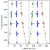 |
Fig. 1. Stretched échelle diagram of KIC 5792889 that does not show any magnetism-induced perturbation. The x-axis is the stretched periods τ modulo ΔΠ1 ≈ 81.6 s. The peaks with S/N > 10 are shown by the grey points (l = 0 and l = 2 modes have been removed). The green ‘+’ stands for the m = 1 modes. The red ‘−’ stands for the m = −1 modes. The blue ‘•’ shows the m = 0 modes. The best-fitting results are plotted by the cross. |
In the presence of a core magnetic field, the oscillation modes undergo a frequency shift that depends on |m| (see Sect. 3). If the core field is strong enough, we anticipate that it can modify the ordering of the m components in a multiplet. This would invalidate our identification of m base on Eq. (9). For all the stars where multiplet asymmetries were detected, we thus investigated alternate identifications of m, assigning m = 0 to the external components of the multiplet. In all these cases, these alternate identifications led to poor fits to the observations, so we ruled out the possibility of having a different ordering of the components in the multipltets.
2.4. Identification of the rotational multiplets
In order to measure multiplet asymmetry, we then needed to identify modes that belong to the same multiplet, that is, modes that share common values of l and n but have different values of m. This step can be complicated when the rotational splitting is comparable to or larger than the frequency spacing between modes of consecutive radial order n. In such cases, the nearest three modes no longer form a single multiplet, making the identification more difficult, as illustrated in Fig. 2 for KIC 7749842.
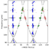 |
Fig. 2. Stretched échelle diagram of KIC 9467102, which does not show any magnetism-induced perturbation. The symbols are the same as Fig. 1. We show this star as an example because its splittings overlap seriously. |
To identify rotational multiplets, we fit an asymptotic expression of mixed modes including rotational effects to the detected modes. For given values of ΔΠ1, εg, q, and fshift, the frequencies of the unperturbed modes are given by solving Eq. (2). We then add rotational splittings to these modes. The rotational splittings δνR can be expressed as
 (10)
(10)
where Ωcore and Ωenv are the mean rotation rates (in unit of angular frequency) in the core and the outer envelope (Goupil et al. 2013; Deheuvels et al. 2014). This expression leads to symmetric rotational multiplets, contrary to what we generally expect for red giants harbouring core magnetic fields. However, if the effects of non-axisymmetry of the magnetic field on the frequency shifts are negligible (as we have assumed in Sect. 2.1), the mode frequencies of azimuthal order m = ±1 are affected in the same way. In this case, the frequency spacing between these two components remains equal to 2δνR, as in the non-magnetic case. We thus used only the m = ±1 modes to perform the fit.
We ran a Markov chain Monte Carlo (MCMC) method to optimise the parameters using the python package EMCEE (Foreman-Mackey et al. 2013). There are in total six parameters that will be optimised. We applied uniform priors to the parameters and defined their ranges for optimisation in the MCMC as shown in Table 2.
The prior ranges of these parameters were determined based on several previous analyses of large samples of red giant stars (Mosser et al. 2017b, 2018; Gehan et al. 2018; Triana et al. 2017). The MCMC algorithm maximises the likelihood function defined as follows:
![Mathematical equation: $$ \begin{aligned} \ln L = -\frac{1}{2}\sum _{m=1, 0, -1} \sum _i\left[\frac{(\nu _{m, i}^\mathrm{obs} -\nu _{m, i}^\mathrm{cal} )^2}{\sigma _{m, i}^2} +\ln \left(2\pi \sigma _{m, i}^2\right)\right], \end{aligned} $$](/articles/aa/full_html/2023/12/aa47260-23/aa47260-23-eq12.gif) (11)
(11)
where  is the ith observed frequency with azimuthal order of m and
  is the calculated frequency. At this stage, the observed frequencies are estimated as the mean of the nearby points in the PSD whose signal-to-noise ratio (S/N) is greater than 10, which is more conservative than the criterion applied in previous studies, such as Mosser et al. (2015).
Currently, we assume that the uncertainty in the observed frequency σm, i is 0.02 μHz. More proper estimates of the mode frequencies and their uncertainties are obtained in Sect. 2.5 by fitting Lorentzian profiles to the PSD.
We ran 14 parallel chains with length of 5000 steps. The first 50% samples are discarded. Finally, we obtained the best-fitting results that give the identification of the multiplets and allow us to run an automated algorithm (in Sect. 2.5) to measure the asymmetric splittings We show the best-fitting results of KIC 9467102 in Fig. A.1. The identified triplets are marked by the horizontal red lines in each panel. Even though there is significant overlap between multiplets, we still can distinguish them. We also find that the splitting identification works well even for the stars with asymmetric splittings.
2.5. Asymmetry measurement
We measured the asymmetries of the identified multiplets by fitting three Lorentzian profiles, whose initial locations are given by the MCMC algorithm in Sect. 2.4. In this fitting for the Lorentzian profile, we can determine the following parameters: the frequencies of the components, the linewidths assuming they are identical for the three components, amplitudes, and inclinations. The amplitudes of the three components were determined by a relation that was modified by inclination (Gizon & Solanki 2003), and the best-fitting results were obtained by maximising the likelihood function defined by Anderson & Duvall (1990). We allowed the m = 0 component to shift freely to reproduce the asymmetry.
Among the stars showing significant multiplet asymmetries, we selected those that share the features expected for magnetic asymmetries, namely:
-
They should have the same sign (either positive or negative) for all multiplets in a given star;
-
They should decrease with frequency (in absolute value);
-
They should be larger for g-dominated modes than for p-dominated modes.
Finally, 13 stars were found to show magnetism-induced asymmetries, including the three stars reported by Li et al. (2022a). Here we show KIC 5696081 as an example. The three panels in Fig. 3 show three continuous asymmetric splittings, whose x-axes are aligned by the m = 1 and m = −1 mode frequencies. The modes in the top and the bottom panels are g-dominated, so they show narrower linewidths and larger asymmetries. While the mode in the middle panel is p-dominated, hence it has wider linewidth and smaller asymmetry. Although the asymmetries vary with different modes, all the asymmetries keep positive. Figure 4 shows the variations in the asymmetry as a function of the frequency in KIC 5696081. We find that they follow all the characteristics expected from a magnetic perturbation (as listed in Sect. 1): the asymmetries are all positive in this star, decrease with frequency, and are smaller for p-dominated modes. We show all the asymmetry measurements in Appendix B.
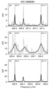 |
Fig. 3. Three continuous asymmetric splittings in KIC 5696081. The top and bottom panels show g-dominated modes while the middle panel displays a p-dominated one. The x-axes of three panels are aligned by the m = 1 and −1 mode frequencies. |
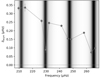 |
Fig. 4. Asymmetries as a function of frequency in KIC 5696081. The dark fringes show where the p-dominated modes are, while the white background shows the locations of g-dominated modes. |
3. Magnetic perturbation and field strength measurement
3.1. Magnetic perturbation
For the stars identified as showing multiplet asymmetries of magnetic origin in Sect. 2.5, we estimated the properties of the field that could reproduce the observations. For this purpose, we followed the approach that we proposed in Li et al. (2022a). We again solved Eq. (2) to obtain the asymptotic expression of mixed mode frequencies, but here the frequencies of pure p and g modes include perturbations arising from rotation and magnetic field.
In the case of axisymmetric fields, or the non-axisymmetric effects are negligible, the frequency perturbation of pure g modes caused by both magnetism and rotation is given by
 (12)
(12)
for m = 0 modes, and
 (13)
(13)
for m = ±1 modes (Li et al. 2022a). In Eqs. (12) and (13), δνg is the magnetic shift for pure g modes at the frequency at maximum power of the oscillations. The asymmetry parameter a is a dimensionless average of  in the oscillation cavity weighted by the second order Legendre polynomial P2(cos θ):
 (14)
(14)
It verifies −0.5 < a < 1, its exact value depending on the latitudinal distribution of  in the oscillation cavity (Li et al. 2022a).
The pure g-mode periods in Eq. (7) can then be rewritten as
 (15)
(15)
For pure p modes, the perturbation only arises from rotation, since the magnetic field being buried inside the star acts mainly on the g-mode parts of mixed modes. The effect on p modes is still negligible even if the magnetic field extends to the p-mode cavity (Mathis et al. 2021). Therefore, the pure p-mode frequency in Eq. (4) is rewritten as
 (16)
(16)
We then solved the asymptotic expressions for m = 1, 0, and −1 respectively,
 (17)
(17)
where  and
and  are the perturbed phases for pure p and g modes. Their expressions are similar to those of the unperturbed phases θp and θg given by Eqs. (3) and (6), but the frequencies of pure p and g modes are now replaced with the perturbed expressions given by Eqs. (12), (13), (15), and (16). Equation (17) can then be solved to obtain the perturbed mixed mode frequencies for any set of parameters characterising (ΔΠ1, q, εg, fshift, Ωcore, Ωenv, a, δνg).
3.2. Fit to the observations
In order to fit our asymptotic expression of mixed modes including rotational and magnetic perturbations to the observations, we ran an MCMC algorithm similar to the one used in Sect. 2.4. The priors for the first six parameters (ΔΠ1, q, εg, fshift, Ωcore, Ωenv) are the same as in Sect. 2.4, and for the two additional parameters a and δνg, we adopted uniform priors and listed its ranges in Table 3.
The same likelihood function as Eq. (11) was used with the uncertainty defined as the quadratic summation of model and observation errors:
 (18)
(18)
When fitting asymptotic expressions of mixed modes to the observations, we found that the optimal solutions have a typical residual spread of 0.02 μHz, which we consider as some residual spread caused by the WKB approximation since the asymptotic expression is not expected to be exact. Hence we included  as additional white noise into the frequency uncertainties to account for the model uncertainty, assuming they are completely uncorrelated. The uncertainties of the mode frequencies (
 ) were obtained in Sect. 2.5.
In the MCMC algorithm, 18 parallel chains were used with length of 4000 steps, and we discarded the first 50% sample results. The posterior distributions of the eight parameters are shown in Fig. 5. We obtained good agreement between the formula including both rotational and magnetic perturbation and the observed asymmetric splittings. To illustrate this, Fig. 6 displays the stretched échelle diagram of KIC 5696081. The dipole triplets form three nearly vertical ridges, and the m = 0 ridge does not fall exactly halfway between m = 1 and m = −1 ridges due to the magnetic perturbations. Our best-fitting frequencies (shown by the crosses) follow the observations well, showing a good agreement between the theory and observations. We display the stretched échelle diagrams of the 13 stars in Appendix B. They show that our fits are in good agreement with the observations and reproduce the asymmetries well.
 |
Fig. 5. Corner diagram of the magnetic fitting of KIC 5696081. The vertical dashed lines mark the median values and ±1σ ranges. |
The best-fitting parameters for all the 13 stars are listed in Table 4. Here we show KIC 5696081 as an example. The corner diagram of the MCMC result is shown in Fig. 5, where the best-fitting result is found with  and
and  . In Fig. 5, as well as the corner diagrams for the other stars in Appendix B, we identify correlations between several parameters. As in the case of non-magnetic red giants, the measurement of ΔΠ1 is strongly anti-correlated with the measurement of εg. This is a direct result from the linear relation given by Eq. (7). We also find a clear correlation between ΔΠ1 and δνg. This can be understood as follows: starting from a best-fit solution, if we increase the value of δνg (that is, if we increase the intensity of the field), the magnetic frequency perturbations increase, which tends to decrease the period spacing between consecutive g modes. Therefore, to correctly reproduce the observations, the asymptotic period spacing of unperturbed g modes ΔΠ1 needs to be increased. Also, the parameters δνg and a are found to be strongly anti-correlated. Again, this was expected. Indeed, using Eqs. (12) and (13), we find that the asymmetry of g-mode multiplets near νmax corresponds to 3aδνg. Therefore, if δνg increases, one needs to decrease a to reproduce the observed asymmetries. Finally, we observe a slight anti-correlation between the measurements of Ωcore and Ωenv. This can be understood from Eq. (10) (even though this relation has not been used in our fits here): in this linear relation, Ωcore and Ωenv are related to the slope and the intercept, respectively, and the measurements of these quantities are not independent.
The asymmetry parameter a generally has larger uncertainties and broader distributions within its prior range (from −0.5 to 1) compared to the other parameters, suggesting that the constraints on a are weaker. The parameter δνg often had an asymmetric distribution, while the other parameters have symmetric distributions and generally tighter constraints.
These stars display normal values for the other parameters of the fits (ΔΠ1, q, εg, and fshift), as shown in Appendix C. Despite the fact that we used non-informative priors for εg, we obtained results that are in line with typical values for other red giants (0.28 ± 0.08; Takata 2016; Mosser et al. 2018).
3.3. Stellar model and field strength
After obtaining the magnetic shift δνg, we can calculate the magnetic field strength in the stellar interior. What we can measure about the magnetic field strength is a weighted integral of the horizontal average of the squared radial magnetic field,  , given by (Li et al. 2022a):
 (19)
(19)
with K(r) the weight function and where ri and ro are the inner and outer turning points of the g-mode cavity, respectively, and μ0 is the vacuum permeability. The core factor ℐ is determined by the internal structure of the star:
 (20)
(20)
where N is the buoyancy frequency and ρ is the local density. The weighted function,
 (21)
(21)
sharply peaks at the hydrogen-burning shell, with a much lower sensitivity in the layers below.
To estimate the intensity of the detected magnetic fields, we needed to characterise the internal structures of these stars (such as the buoyancy frequency N and the density profile ρ). For this purpose, we adopted the seismology-modelling pipeline and the model grid introduced by Li et al. (2022b) to search for the best-fitting models. The input constraints were based on global parameters, such as effective temperature, luminosity, and metallicity, which were reported by Berger et al. (2020) and listed in Table 5. We also used the observed radial-mode frequencies given by Li et al. (2022b), and the asymptotic period spacing of g modes (ΔΠ1) measured by this work as additional constraints. By applying the pipeline, we determined the best-fitting structural model, whose parameters (masses, ages, and radii) are listed in Table 5.
Values and their uncertaintiers of Teff, log L/L⊙, and [Fe/H] that were used to constrain the theoretical models.
Using our best-fit stellar models, we could derive estimates of the core factor ℐ, and we were thus able to obtain measurements of the average radial magnetic fields  using Eq. (19) (see Table 5). We found field strengths ranging from about 20 kG to 150 kG.
Since this work and Li et al. (2022a) used different approaches in the stellar modelling and the fitting of the asymptotic expression of mixed mode frequencies to the observations, there are slight differences in the inferred field strengths for the three stars that they have in common. In Fig. 7, we compared the two sets of results and found that the field strengths derived by both works are generally consistent, with slightly larger strengths obtained in this work. For KIC 7518143 and KIC 8684542, they have consistent field strengths within 1-σ ranges. While for KIC 11515377, the field strength obtained by this work is approximately 30% times larger than the strength by Li et al. (2022a), though still within the 2-σ range. The ratios between the field strength and the critical field strength show good agreement between the two sets of results, likely due to this ratio being more sensitive to the stellar structure rather than the observed frequencies or the fitting strategies.
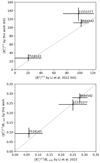 |
Fig. 7. Result comparison between this work and Li et al. (2022a). Top panel: measured field strengths by this work and by Li et al. (2022a). Bottom: the ratio between the measured field strengths and the critical strengths. The dotted lines show 1:1 relations. The value of the field strength of KIC 7518143 reported by Li et al. (2022a) is smaller than 41 kG, while we use the median here (20.5 kG). |
In Appendix D, we also offer a linear relation between ℐ and ΔΠ1. This relation can be used for model-independent calculations of field strength, particularly when a best-fitting stellar model is unavailable.
4. Discussion
4.1. Asymmetry parameter and magnetic shift
Figure 8 displays the relation between the asymmetry parameter a and the magnetic shift δνg. We find that there is no obvious correlation between these two parameters and there is also no correlation with the period spacing ΔΠ1. Figure 9 shows the relation between the asymmetry parameter a and the field strength of our sample, and we still do not find any correlation between them, meaning that the field strength does not correlate with the field topology.
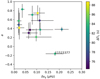 |
Fig. 8. Relation between the asymmetry parameter a and the magnetic shift δνg. KIC 11515377 is the only star that shows negative asymmetries. |
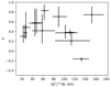 |
Fig. 9. Relation between the asymmetry parameter a and the field strength. |
The asymmetry parameter a reaches 1 when the field is entirely concentrated to the poles and it reaches −0.5 when the field is concentrated to the equator. Dipolar fields have values of a ranging from −0.2 (corresponding to a dipolar field aligned with the equator) to 0.4 (corresponding to a dipolar field aligned with the rotation axis). The asymmetry parameter can also vanish, even in the presence of a strong field, for example if a dipolar field is inclined by about 55° with respect to the rotation axis or if the latitudinal variations of  only occur at length scales much smaller than the star radius (Li et al. 2022a). Most of the stars exhibit a values between 0.2 and 0.8. KIC 11515377 is the only star that shows negative asymmetries, which lead to a close to −0.2. This suggests that this configuration might be rarer among red giants. We note the diversity of the values obtained for the asymmetry parameter a, which clearly shows that the core fields of red giants have various horizontal geometries. In some stars, the posterior probabilities for the asymmetry parameter a nearly vanish below 0.4, which means that for these stars the magnetic fields are more sharply concentrated on the poles than a purely dipolar field aligned with the rotation axis. Our measurements of a will be useful to constrain future models of red giant core magnetic fields.
4.2. Core and envelope rotation rates
We display the relation between Ωcore and ΔΠ1 in Fig. 10. The figure shows that the rotation rates of our stars are typical for red giants and are consistent with those of other studies (shown as the grey circles by Gehan et al. 2018). Our observations thus suggest that these stars have not experienced significantly different histories of angular momentum transport compared to other red giant stars. We note that this does not contradict the hypothesis that magnetic fields could be responsible for angular momentum transport in red giants because we cannot exclude that magnetic fields currently escaping detection might exist in other red giants.
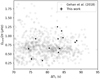 |
Fig. 10. The core rotation rates Ωg as a function of ΔΠ1. The black dots are the stars in this work, and the grey circles are reported by Gehan et al. (2018). |
We compared our measurements of the core rotation rates with those of Gehan et al. (2018) for the five stars in our sample that were also in their study. We find that our results are consistent in four stars (KIC 7518143, 6936091, 11515377, and 8540034), while a large discrepancy appears in KIC 8684542. The reason for the consistency is that the magnetism-induced perturbation does not change the frequency separation between m = 1 and m = −1 modes, hence it does not affect the measurements of splittings if the mode identification is correct. However, the discrepancy for KIC 8684542 arises because only symmetric rotational splittings were considered in the previous work, which resulted in an incorrect identification of the splitting of m = 1 and −1 modes (see the online peer review file of Li et al. 2022a).
The top panel of Fig. 11 displays the measurements of the envelope rotation rates as a function of their model-inferred radii. The method used in Sect. 3 does not require the use of the ζ function, which is different from the method used by Li et al. (2022a) to measure the internal rotation. Consequently, the envelope rotation rates obtained using the current method exhibit differences compared to the results reported by Li et al. (2022a). Due to the expansion of the envelopes, red giant stars show very slow envelope rotations. Most of the stars have surface rotation rates around 0.02 μHz, equivalent to about ∼600 d. KIC 7518143 has the fastest surface rotation rate with a rotation period of about 170 days. For the two stars KIC 6936091 and KIC 9589420, with relatively large radii inferred from the modelling (larger than six solar radii), the rotation rates are slower than the detection limit of the seismic signal, resulting in surface rotation rates that are compatible with zero within 1σ ranges.
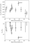 |
Fig. 11. Top panel: surface rotation rates as a function of model-inferred radii. Bottom panel: variations in the ratio Ωcore/Ωenv with stellar radii. |
The bottom panel of Fig. 11 shows the ratio between the core and the envelope rotations (Ωcore/Ωenv), which represents the level of differential rotation. For the two stars with near-zero envelope rotations (with radii larger than 6 solar radii), we can only obtain a lower limit to this ratio. Among the remaining stars, we find that the rotation ratio lies between 10 and 100. Interestingly, KIC 7518143, the star with the fastest envelope rotation, also shows a slow core-rotation rate, which leads to the rotation ratio Ωcore/Ωenv is only around 4. This finding suggests that a strong transfer of angular momentum occurs inside the star, but the relation with magnetic field is unclear, as the measured field strength of this star is not the strongest.
4.3. Comparison with critical field strength
Fuller et al. (2015) showed that magnetic fields that exceed a critical value Bc can prevent the propagation of gravity waves. This phenomenon was invoked as a possible explanation for the suppression of l = 1 mixed modes in a fraction of red giant stars (see also in Stello et al. 2016). Fuller et al. (2015) suggested that when the g-mode cavity harbours a magnetic field stronger than Bc, all the mode energy that reaches the core is dissipated, leading to modes that have a pure p-like behaviour. This interpretation was challenged by Mosser et al. (2017a), who found that for red giants that show only partially suppressed dipole modes, the modes still have a g-like character. This question is currently under debate. Even though we do not yet have a clear picture of how global oscillation modes are affected by a magnetic field exceeding Bc, it is clear that it will have an impact. We thus compared the measured field strength to the critical field strength, which we computed using our best-fit stellar models. In practice, this critical field varies as a function of radius. The minimum appears at the hydrogen-burning shell (HBS), as given by
 (22)
(22)
where ρhbs, rhbs, and Nhbs are the density, radius, and the Brunt-Väisälä frequency at the hydrogen-burning shell. Using our optimal stellar models, we computed Bc, min for the 13 stars of our sample. The obtained values ore listed in Table 5.
Using the values listed in Table 5, we can calculate the ratio between the measured and critical field strengths as a function of ΔΠ1. The ratios range from approximately 0.1–0.3. It is important to note that the critical field strength varies with radius, and we use the minimum value, which occurs at the hydrogen-burning shell and is consistent with the layer where we measure the field strength. Additionally, the measured field strength is the average over the weight function K(r), which means that some contribution from the field strength inside the hydrogen-burning shell is also included (see extended data Fig. 1 in Li et al. 2022a). Therefore, the reported ratios may not be representative of the fields ratio at the location of hydrogen-burning shell.
Figure 12 shows the observed and critical field strength with evolution, indicated by the mixed mode density  (Gehan et al. 2018). It is evident from Fig. 12 that the critical field strengths tend to decrease as stars evolve along the red giant branch (this was already shown by Fuller et al. 2015). We also observe an overall decrease in the observed field strengths with the evolution (albeit with relatively large scatter). This is in contrast to the theoretical prediction that the field strength should increase with evolution, assuming the magnetic flux is conserved while the core contracts. However, if the field strength exceeds the critical field strength, the energy of gravity waves is thought to be completely transferred to Alfvén waves, and we cannot observe any dipole mixed modes (Fuller et al. 2015). Moreover, a strong field leads to a curvature in the stretched échelle diagram (Li et al. 2022a; Bugnet 2022; Deheuvels et al. 2023), which could obscure the observations. Therefore, only a field that is ∼10% to ∼30% of the critical field strength can generate observable asymmetric splittings. This could explain why the decrease in the detected field strength with evolution seems to follow the decrease in the critical field Bc (Fig. 12).
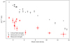 |
Fig. 12. Field strength as a function of mixed mode density. The red hexagons with errorbars are the field strengths of the 13 stars reported by this work, and the black dots are their critical field strengths. The grey vertical arrows show the lower limits of the field strengths reported by Deheuvels et al. (2023), where the stars do not show any asymmetric splittings, but only m = 0 curved ridges in their stretched échelle diagrams. |
Deheuvels et al. (2023) reported 11 stars showing curved stretched échelle diagrams caused by their central magnetic fields. In this case, only the lower limit of the field strengths are derived. We plot the results by the grey vertical arrows in Fig. 12, and find that they also follow a decreasing trend with evolution but with much stronger field strengths. Figure 12 reveals a large gap of field strength between the stars exhibiting asymmetric splittings, as seen in this work, and those with curved stretched échelle diagrams, as observed by Deheuvels et al. (2023). The search for such power spectra may be hindered by an observational bias, as explained in Sect. 4.6.
4.4. Origin of the fields
Figure 13 depicts the measured field strengths plotted against model-inferred age and mass. In the top panel, most stars have ages smaller than 6 Gyr and the field strengths of these stars show large scatter. However, for the two stars with longer ages (between 8 and 9 Gyr), the field strengths are small. As stellar age is strongly related to mass, we examined the correlation between field strength and mass in the bottom panel of Fig. 13. We find that most stars have masses larger than 1.3 M⊙, meaning that they had convective cores in their main-sequence stages and can generate strong central fields by the dynamo processes. Since the Ohmic timescale, over which magnetic field dissipate, is longer than the evolution timescale (Cantiello et al. 2016), such fields could survive until the red-giant phase, where they may relax into stable mixed poloidal-toroidal configurations (Braithwaite & Spruit 2004).
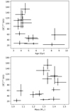 |
Fig. 13. Top panel: field strengths with model-inferred ages. Bottom panel: field strengths but with model-inferred masses. |
However, we observed two stars with lower masses (1.08 M⊙ for KIC 4458118 and 1.04 M⊙ for KIC 6936091). Our best-fit models for these stars had a radiative core during the bulk of their main sequence, which challenges the interpretation that their central fields may have been generated by the core dynamo. To further study the origin of the field, we calculated the mass and the radius of the convective core at the beginning of stellar life. For the two low-mass stars (KIC 4458118 and 6936091), we found that they show convective cores with masses of ∼12% of the total stellar masses at the very beginning of its evolution (∼30 Myr), owing to the burning of 3He and 12C outside of equilibrium (Deheuvels et al. 2010). However, the convective core was too small to reach the shell that is currently burning hydrogen in red-giant phase (which is located at about ∼20% of the total stellar masses). Even though the hydrogen-burning shell in these two stars was never convective, we cannot rule out the dynamo origin because the weight function K(r) involved in the expression of the measured field has a contribution from the deeper layers of the star. If we assume that the magnetic field is confined to the layers that were convective at the beginning of the main sequence (i.e., the layers whose mass is smaller than 12% of the total mass), we find that fields of ∼300 kG for KIC 4458118 and ∼200 kG for KIC 6936091 are needed to reproduce the observations. These values are several times larger than the values given in Table 5. However, we cannot exclude that such fields might result from a dynamo process in main-sequence cores because these field strengths remain compatible with the amplitudes predicted by numerical simulations of core convection (Brun et al. 2005) and dynamo scaling laws (Bugnet et al. 2021). In addition, the determination of convective core size still shows an uncertainty due to the poorly-understanding internal chemical mixing process (e.g., Johnston 2021). Another possibility for the origin of the magnetic field is that it is inherited from a fossil field.
4.5. Ongoing dynamo versus stable fields
The ratio between the Alfvén frequency  and the rotation rate Ω is an important parameter of the dynamical interactions between magnetic field and rotation. Its value can provide some clues about the nature of the detected magnetism. We computed this ratio at the HBS of the 13 red giants and, as shown in Fig. 14, found that it is comprised between 0.05 and 0.25.
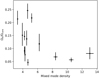 |
Fig. 14. Ratio of the Alfvèn frequency |

A first consequence is that a Tayler–Spruit dynamo is probably not presently at work in these layers. Indeed, the Fuller et al. (2019) model of the Tayler–Spruit dynamo finds that ΩA/Ω should scale with (Ω/N)5/3 where N, the Brunt-Väisälä frequency, measures the strength of stable stratification in radiative zones. As (Ω/N)5/3 ∼ 10−7 at the HBS of a typical 1.2 M⊙ and 4 R⊙ star at the base of the red giant branch (Fuller et al. 2019), the predicted ΩA/Ω are extremely small and thus incompatible with our measurements.
The observed ratios are rather compatible with a stable magnetic field configuration. Indeed, as anticipated in Spruit (1999), numerical studies of a poloidal magnetic field embedded in a differentially rotating radiative zone have shown that, if the ratio ΩA/Ωcore exceeds a certain value, the field is not affected by instabilities and evolves towards stable configurations while being only subjected to ohmic dissipation (Jouve et al. 2015, 2020; Gouhier et al. 2022). The values obtained in numerical simulations vary between 10−3 for a free differential rotation (Jouve et al. 2020) and 10−2 for a differential rotation forced by a radial flow simulating a star contraction (Gouhier et al. 2022). Another argument in favour of a stable magnetic field configuration comes from the magnetic fields observed at the surface of intermediate-mass and massive main-sequence stars. In this mass range, the so-called fossil magnetic fields are stable at least over decades and their ΩA/Ω ratio, computed at the star’s surface, is always greater than ∼1 (Aurière et al. 2007).
4.6. Observational biases
Our method of analysis of Kepler data presented in Sect. 2 leads to several observational biases that need to be acknowledged.
4.6.1. Limitation on the measurable field strength
As mentioned in Sect. 2.1, we have assumed that the magnetic field is not strong enough to significantly alter the regularity of g-mode period spacings. Deheuvels et al. (2023) estimated the magnetic intensity threshold Bth above which deviations from the regular period spacing of pure g modes become detectable (see their Appendix B). They found that Bth follows a similar decreasing trend with evolution as that of the critical field Bc. Overall, a magnetic field that exceeds about 40% of the critical field should produce significant deviations. We can thus expect that our method may start failing for field strengths above 0.4 Bth. This could at least partly explain the gap that we found between the field measurements in this work and those obtained by Deheuvels et al. (2023).
Additionally, we assumed in Sect. 2.3 that the magnetic asymmetries are not large enough to push the m = 0 component of the multiplets outside the interval formed by m = ±1 components. This phenomenon occurs if νg mode, m = 0 < νg mode, m = +1 when a > 0, and if νg mode, m = 0 > νg mode, m = −1 when a < 0. Using Eqs. (12) and (13), one finds that near νmax, this condition is equivalent to
 (23)
(23)
For the 13 stars of our sample, the quantity on the left-hand-side of Eq. (23) takes values between 0.03 and 0.36. It is not straightforward to translate the condition given by Eq. (23) in terms of a constraint on the field intensity because it depends on properties that vary from star to star (namely a, ℐ, νmax, and Ωcore). If we consider the values of these parameters that were obtained for the stars of our sample, we find that a change in the ordering of components in a multiplet would occur for these stars if the field strengths were multiplied by a factor ranging from 1.6 to 5.8. This corresponds to field intensities that are intermediate between the measured values and the critical field strengths. We thus conclude that our assumption that the m = 0 component lies between the m = ±1 components could partly explain the lack of red giants with measured fields closer to the critical field strength.
4.6.2. Non-axisymmetric effects
Equations (12) and (13) hold when the non-axisymmetric effects of magnetic fields are negligible. This is true (i) if  is axisymmetric, but also (ii) if the ratio b between the magnetic frequency and the rotational splitting (b = 4πδνg/Ωcore) is smaller than ∼1 (see the supplementary material S2.7 in Li et al. 2022a). Our results in Table 4 show that the ratio b is much smaller than one. The stars with the largest values of b are KIC 8684542 (b = 0.64 ± 0.09) and KIC 11515377 (b = 0.56 ± 0.12), the other stars having b values below ∼0.35. Hence, we state that case (ii) is valid for our stars, so that even if
  is non-axisymmetric, we still cannot see any significant non-axisymmetric effect in the oscillation spectra.
As mentioned in Sect. 2.1, when b ≳ 1, non-axisymmetric magnetic fields can produce up to nine components for dipole modes (Li et al. 2022a). Dedicated methods need to be devised and applied to search for such features in the oscillation spectra of red giants. This work is currently undertaken by our team and will be the subject of a next publication. Meanwhile, our assumption that non-axisymmetric effects are weak limits the strength of detectable fields. Similarly to Sect. 4.6.1, the condition b ≳ 1 cannot directly be translated in terms of field strength. We thus estimated the minimal field strengths that the stars of our sample should have in order to produce significant non-axisymmetric effects. We found that the measured fields would need to be multiplied by a factor ranging from 1.2 to 5.4. Again, this corresponds to field intensities that lie between the measurements obtained in this study and those found by Deheuvels et al. (2023). Taking non-axisymmetric effects into account could thus populate the gap observed in Fig. 12.
5. Conclusions
In this study, we conducted a systematic search for magnetism-induced asymmetric splittings in Kepler data. This work constrains the strength and topology of the magnetic fields, hence it can be used in future numerical simulations and provides the possibility to further investigate the evolution of magnetic fields and their interaction with stellar rotation.
We successfully identified 13 stars (including the three stars previously reported by Li et al. 2022a) exhibiting clear multiplet asymmetries with properties matching those expected in the presence of a core magnetic field. Notably, we found that only one star (KIC 11515377) displayed negative asymmetries, while the remaining stars exhibited positive asymmetries. By fitting an asymptotic expression of mixed mode frequencies including rotational and magnetic effects to the observations, we were able to measure the magnetic frequency shift δνg (which is related to the field strength), and the asymmetry parameter a (which yields constraints on the field topology).
Using the best-fitting stellar structure model, we were able to measure the average radial field strength in the core ( ) for the 13 stars. These field strengths were found to lie between approximately 20 and 150 kG, with maximal sensitivity in the vicinity of the hydrogen-burning shells. These values represent about 10%–30% of the critical field strength above which gravity modes are no longer expected to propagate in the core (Fuller et al. 2015).
We also obtained estimates of the asymmetry parameter a, which provides a horizontal average of  weighted by the second-order Legendre polynomial (see Eq. (14)). For the 13 stars, we found values of a between about −0.2 and 0.95, nearly spanning the entire possible range for this parameter (−0.5 ≤ a ≤ 1). We recall that large negative values of a are reached for fields that are concentrated near the equator, while large positive values of a correspond to fields concentrated on the poles. Our results thus show that the core fields of red giants have various horizontal geometries. For some stars, we find values of a that significantly exceed 0.4, which is the highest value that can be obtained with a dipolar magnetic field. This means that for these stars, the fields are more sharply concentrated on the poles than a pure dipolar field aligned with the rotation axis. The fact that a negative value of a was obtained for only one star (KIC 11515377) suggests that this configuration might be rare among red giants.
In agreement with the results of Deheuvels et al. (2023), we found that the magnetic field strength in the core of red giants decreases with evolution (see Fig. 12). This is in contradiction with the general expectation that the contraction of the core should increase the magnetic field, if we assume a conservation of the magnetic flux. As was already pointed out in Deheuvels et al. (2023), the observed decrease seems to follow the overall decrease of the critical field strength Bc with evolution. One possible interpretation is thus that for a given star, the core magnetic field increases with evolution until it reaches Bc. At this point, gravity waves no longer propagate in the core so that dipole modes do not have a mixed behaviour, and therefore core magnetic fields can no longer be detected. This could account for the observed decrease in the measured field strength, although further work is clearly needed to test this interpretation.
This work presents a larger sample of red giant stars with central magnetic fields, comprising 13 stars out of approximately 1200 red giant stars with triplets. The prevalence of such magnetic fields is thus currently found to be only 1%. Stello et al. (2016) claimed that about 5–15% of red giants in the mass range of our sample are magnetised based on the assumption that suppressed dipole mixed modes are caused by magnetic fields exceeding the critical field strength. So far, this assumption remains challenged (Mosser et al. 2017a), but if it were correct, the stars of Stello et al. (2016) (which lie in a different range of field intensities compared to this work) could be added to the list of magnetic red giants. The low prevalence of magnetic giants in our sample may be partly due to observational biases related to the analysis method that we adopted in this study. We assumed that the field strength was not strong enough to significantly alter the regularity in the g-mode period spacings, modify the ordering of the components within dipole multiplets, or produce detectable effects related to the non-axisymmetric component of the magnetic field. We estimated that field intensities exceeding the measured field strengths by a factor of a few would be enough to make at least one of these assumptions invalid. Therefore, the present study might miss stars with stronger core fields. We also stress that in this study, magnetic giants have been identified by searching for multiplet asymmetries. This method can thus not detect magnetic fields with horizontal geometries that correspond to vanishing values of a.
Regarding the origin of the detected fields, one of the main scenarios is that they were produced by a dynamo in the main-sequence convective core. After the end of the main sequence, these fields would have relaxed into stable configurations (Braithwaite & Spruit 2004), undergoing only weak Ohmic diffusion (Cantiello et al. 2016). In this study, we found magnetic fields in two low-mass stars ( for KIC 6936091, and
  for KIC 4458118), who had a small convective core only at the very beginning of the main sequence, owing to nuclear reactions outside of equilibrium. These convective cores never reached the layers where our magnetic field measurements have maximal sensitivity, namely the hydrogen-burning shell. Assuming that the core magnetic field is confined to the layers that were once convective, we found that field strengths of 200–300 kG need to be invoked. These intensities remain compatible with order-of-magnitude predictions of field strengths produced by dynamo in main-sequence convective cores (Brun et al. 2005; Bugnet et al. 2021). Another possible interpretation is that the detected fields might be inherited from fossil magnetic fields.
Internal magnetic fields have been proposed as a candidate to provide additional transport of angular momentum inside stars. In this study, we were also able to measure average core rotation rates for the 13 stars. We found values that are in line with the typical rotation rates of red giant cores, as obtained by Gehan et al. (2018). This suggests that the stars of our sample do not undergo enhanced angular momentum redistribution compared to other red giants. This does not rule out magnetic fields as the origin of the angular momentum transport in red giants, as other red giants may harbour core magnetic fields that were not detected, either because of our observational biases or because they are below the detection threshold. The relatively high ratios between the Alfvèn frequency and the rotation rate rule out that the observed fields are fed by an ongoing Tayler–Spruit dynamo. They rather point towards fields that have settled into stable configurations.
We fitted a Lorentzian profile to each detected l = 0 and l = 2 modes to obtain their frequencies (Anderson & Duvall 1990).
Acknowledgments
The authors acknowledge support from the project BEAMING ANR-18-CE31-0001 of the French National Research Agency (ANR) and from the Centre National d’Études Spatiales (CNES). Gang Li received funding from the KU Leuven Research Council under grant C16/18/005: PARADISE. G.L. expresses his gratitude for support from the Dick Hunstead Fund for Astrophysics during his visit to The University of Sydney. T.L. acknowledges support from the Joint Research Fund in Astronomy (U2031203) under cooperative agreement between the National Natural Science Foundation of China (NSFC) and Chinese Academy of Sciences (CAS), NSFC grants (12090040, 12090042), and the European Research Council (ERC) under the European Union’s Horizon 2020 research and innovation programme (CartographY GA. 804752). This paper includes data collected by the Kepler mission and obtained from the MAST data archive at the Space Telescope Science Institute (STScI). Funding for the Kepler mission is provided by the NASA Science Mission Directorate. STScI is operated by the Association of Universities for Research in Astronomy, Inc., under NASA contract NAS 5-26555.
References
- Aerts, C., Christensen-Dalsgaard, J., & Kurtz, D. W. 2010, Asteroseismology (Dordrecht: Springer) [Google Scholar]
- Anderson, E. R., Duvall, Thomas L. J., & Jefferies, S. M., 1990, ApJ, 364, 699 [NASA ADS] [CrossRef] [Google Scholar]
- Aurière, M., Wade, G. A., Silvester, J., et al. 2007, A&A, 475, 1053 [NASA ADS] [CrossRef] [EDP Sciences] [Google Scholar]
- Aurière, M., Konstantinova-Antova, R., Charbonnel, C., et al. 2015, A&A, 574, A90 [Google Scholar]
- Beck, P. G., Montalban, J., Kallinger, T., et al. 2012, Nature, 481, 55 [Google Scholar]
- Bedding, T. R. 2014, in Asteroseismology, eds. P. L. Pallé, & C. Esteban (Cambridge, UK: Cambridge University Press), 60 [Google Scholar]
- Bedding, T. R., Huber, D., Stello, D., et al. 2010, ApJ, 713, L176 [Google Scholar]
- Bedding, T. R., Mosser, B., Huber, D., et al. 2011, Nature, 471, 608 [Google Scholar]
- Belkacem, K., Marques, J. P., Goupil, M. J., et al. 2015, A&A, 579, A30 [NASA ADS] [CrossRef] [EDP Sciences] [Google Scholar]
- Benomar, O., Takata, M., Shibahashi, H., Ceillier, T., & García, R. A. 2015, MNRAS, 452, 2654 [Google Scholar]
- Berger, T. A., Huber, D., van Saders, J. L., et al. 2020, AJ, 159, 280 [Google Scholar]
- Blazère, A., Petit, P., Lignières, F., et al. 2016, A&A, 586, A97 [NASA ADS] [CrossRef] [EDP Sciences] [Google Scholar]
- Borucki, W. J., Koch, D., Basri, G., et al. 2010, Science, 327, 977 [Google Scholar]
- Braithwaite, J., & Spruit, H. C. 2004, Nature, 431, 819 [Google Scholar]
- Braithwaite, J., & Spruit, H. C. 2017, R. Soc. Open Sci., 4 [Google Scholar]
- Brun, A. S., Browning, M. K., & Toomre, J. 2005, ApJ, 629, 461 [Google Scholar]
- Bugnet, L. 2022, A&A, 667, A68 [NASA ADS] [CrossRef] [EDP Sciences] [Google Scholar]
- Bugnet, L., Prat, V., Mathis, S., et al. 2021, A&A, 650, A53 [NASA ADS] [CrossRef] [EDP Sciences] [Google Scholar]
- Cantiello, M., Mankovich, C., Bildsten, L., Christensen-Dalsgaard, J., & Paxton, B. 2014, ApJ, 788, 93 [Google Scholar]
- Cantiello, M., Fuller, J., & Bildsten, L. 2016, ApJ, 824, 14 [NASA ADS] [CrossRef] [Google Scholar]
- Ceillier, T., Eggenberger, P., García, R. A., & Mathis, S. 2013, A&A, 555, A54 [NASA ADS] [CrossRef] [EDP Sciences] [Google Scholar]
- Chontos, A., Sayeed, M., & Huber, D. 2021, Posters fromthe TESS Science Conference II (TSC2), 189 [Google Scholar]
- Deheuvels, S., Michel, E., Goupil, M. J., et al. 2010, A&A, 514, A31 [NASA ADS] [CrossRef] [EDP Sciences] [Google Scholar]
- Deheuvels, S., Doğan, G., Goupil, M. J., et al. 2014, A&A, 564, A27 [NASA ADS] [CrossRef] [EDP Sciences] [Google Scholar]
- Deheuvels, S., Ballot, J., Beck, P. G., et al. 2015, A&A, 580, A96 [NASA ADS] [CrossRef] [EDP Sciences] [Google Scholar]
- Deheuvels, S., Ouazzani, R. M., & Basu, S. 2017, A&A, 605, A75 [NASA ADS] [CrossRef] [EDP Sciences] [Google Scholar]
- Deheuvels, S., Ballot, J., Eggenberger, P., et al. 2020, A&A, 641, A117 [EDP Sciences] [Google Scholar]
- Deheuvels, S., Ballot, J., Gehan, C., & Mosser, B. 2022, A&A, 659, A106 [NASA ADS] [CrossRef] [EDP Sciences] [Google Scholar]
- Deheuvels, S., Li, G., Ballot, J., & Lignières, F. 2023, A&A, 670, L16 [NASA ADS] [CrossRef] [EDP Sciences] [Google Scholar]
- Donati, J. F., & Landstreet, J. D. 2009, ARA&A, 47, 333 [Google Scholar]
- Eggenberger, P., Montalbán, J., & Miglio, A. 2012, A&A, 544, L4 [NASA ADS] [CrossRef] [EDP Sciences] [Google Scholar]
- Eggenberger, P., Lagarde, N., Miglio, A., et al. 2017, A&A, 599, A18 [CrossRef] [EDP Sciences] [Google Scholar]
- Eggenberger, P., Deheuvels, S., Miglio, A., et al. 2019, A&A, 621, A66 [NASA ADS] [CrossRef] [EDP Sciences] [Google Scholar]
- Ferrario, L., Wickramasinghe, D., & Kawka, A. 2020, Adv. Space Res., 66, 1025 [NASA ADS] [CrossRef] [Google Scholar]
- Foreman-Mackey, D., Hogg, D. W., Lang, D., & Goodman, J. 2013, PASP, 125, 306 [Google Scholar]
- Fuller, J., Lecoanet, D., Cantiello, M., & Brown, B. 2014, ApJ, 796, 17 [Google Scholar]
- Fuller, J., Cantiello, M., Stello, D., Garcia, R. A., & Bildsten, L. 2015, Science, 350, 423 [Google Scholar]
- Fuller, J., Piro, A. L., & Jermyn, A. S. 2019, MNRAS, 485, 3661 [NASA ADS] [Google Scholar]
- García, R. A., Ceillier, T., Salabert, D., et al. 2014, A&A, 572, A34 [NASA ADS] [CrossRef] [EDP Sciences] [Google Scholar]
- Gehan, C., Mosser, B., Michel, E., Samadi, R., & Kallinger, T. 2018, A&A, 616, A24 [NASA ADS] [CrossRef] [EDP Sciences] [Google Scholar]
- Gizon, L., & Solanki, S. K. 2003, ApJ, 589, 1009 [Google Scholar]
- Gomes, P., & Lopes, I. 2020, MNRAS, 496, 620 [NASA ADS] [CrossRef] [Google Scholar]
- Gough, D. O., & Thompson, M. J. 1990, MNRAS, 242, 25 [Google Scholar]
- Gouhier, B., Jouve, L., & Lignières, F. 2022, A&A, 661, A119 [NASA ADS] [CrossRef] [EDP Sciences] [Google Scholar]
- Goupil, M. J., Mosser, B., Marques, J. P., et al. 2013, A&A, 549, A75 [NASA ADS] [CrossRef] [EDP Sciences] [Google Scholar]
- Grosjean, M., Dupret, M. A., Belkacem, K., et al. 2014, A&A, 572, A11 [CrossRef] [EDP Sciences] [Google Scholar]
- Hasan, S. S., Zahn, J. P., & Christensen-Dalsgaard, J. 2005, A&A, 444, L29 [NASA ADS] [CrossRef] [EDP Sciences] [Google Scholar]
- Hekker, S., & Christensen-Dalsgaard, J. 2017, A&ARv, 25, 1 [Google Scholar]
- Hermes, J. J., Gänsicke, B. T., Kawaler, S. D., et al. 2017, ApJS, 232, 23 [Google Scholar]
- Huber, D., Stello, D., Bedding, T. R., et al. 2009, Commun. Asteroseismol., 160, 74 [Google Scholar]
- Johnston, C. 2021, A&A, 655, A29 [NASA ADS] [CrossRef] [EDP Sciences] [Google Scholar]
- Jouve, L., Gastine, T., & Lignières, F. 2015, A&A, 575, A106 [NASA ADS] [CrossRef] [EDP Sciences] [Google Scholar]
- Jouve, L., Lignières, F., & Gaurat, M. 2020, A&A, 641, A13 [EDP Sciences] [Google Scholar]
- Kjeldsen, H., & Bedding, T. R. 1995, A&A, 293, 87 [NASA ADS] [Google Scholar]
- Kurtz, D. W., Saio, H., Takata, M., et al. 2014, MNRAS, 444, 102 [Google Scholar]
- Kuszlewicz, J. S., Hon, M., & Huber, D. 2023, ApJ, 954, 152 [NASA ADS] [CrossRef] [Google Scholar]
- Landstreet, J. D. 1992, A&ARv, 4, 35 [NASA ADS] [CrossRef] [Google Scholar]
- Li, G., Van Reeth, T., Bedding, T. R., et al. 2020, MNRAS, 491, 3586 [Google Scholar]
- Li, G., Deheuvels, S., Ballot, J., & Lignières, F. 2022a, Nature, 610, 43 [NASA ADS] [CrossRef] [Google Scholar]
- Li, T., Li, Y., Bi, S., et al. 2022b, ApJ, 927, 167 [NASA ADS] [CrossRef] [Google Scholar]
- Li, Y., Bedding, T. R., Murphy, S. J., et al. 2022c, Nat. Astron., 6, 673 [NASA ADS] [CrossRef] [Google Scholar]
- Lignières, F., Petit, P., Böhm, T., & Aurière, M. 2009, A&A, 500, L41 [CrossRef] [EDP Sciences] [Google Scholar]
- Loi, S. T. 2020, MNRAS, 493, 5726 [CrossRef] [Google Scholar]
- Loi, S. T. 2021, MNRAS, 504, 3711 [NASA ADS] [CrossRef] [Google Scholar]
- Lomb, N. R. 1976, Ap&SS, 39, 447 [Google Scholar]
- Lund, M. N., Silva Aguirre, V., Davies, G. R., et al. 2017, ApJ, 835, 172 [Google Scholar]
- Marques, J. P., Goupil, M. J., Lebreton, Y., et al. 2013, A&A, 549, A74 [NASA ADS] [CrossRef] [EDP Sciences] [Google Scholar]
- Mathis, S., & Bugnet, L. 2023, A&A, 676, L9 [NASA ADS] [CrossRef] [EDP Sciences] [Google Scholar]
- Mathis, S., Bugnet, L., Prat, V., et al. 2021, A&A, 647, A122 [EDP Sciences] [Google Scholar]
- Mosser, B., Barban, C., Montalbán, J., et al. 2011, A&A, 532, A86 [NASA ADS] [CrossRef] [EDP Sciences] [Google Scholar]
- Mosser, B., Elsworth, Y., Hekker, S., et al. 2012a, A&A, 537, A30 [NASA ADS] [CrossRef] [EDP Sciences] [Google Scholar]
- Mosser, B., Goupil, M. J., Belkacem, K., et al. 2012b, A&A, 548, A10 [NASA ADS] [CrossRef] [EDP Sciences] [Google Scholar]
- Mosser, B., Vrard, M., Belkacem, K., Deheuvels, S., & Goupil, M. J. 2015, A&A, 584, A50 [NASA ADS] [CrossRef] [EDP Sciences] [Google Scholar]
- Mosser, B., Belkacem, K., Pinçon, C., et al. 2017a, A&A, 598, A62 [NASA ADS] [CrossRef] [EDP Sciences] [Google Scholar]
- Mosser, B., Pinçon, C., Belkacem, K., Takata, M., & Vrard, M. 2017b, A&A, 600, A1 [NASA ADS] [CrossRef] [EDP Sciences] [Google Scholar]
- Mosser, B., Gehan, C., Belkacem, K., et al. 2018, A&A, 618, A109 [NASA ADS] [CrossRef] [EDP Sciences] [Google Scholar]
- Ouazzani, R. M., Marques, J. P., Goupil, M. J., et al. 2019, A&A, 626, A121 [NASA ADS] [CrossRef] [EDP Sciences] [Google Scholar]
- Pinçon, C., Belkacem, K., & Goupil, M. J. 2016, A&A, 588, A122 [NASA ADS] [CrossRef] [EDP Sciences] [Google Scholar]
- Rüdiger, G., Gellert, M., Spada, F., & Tereshin, I. 2015, A&A, 573, A80 [NASA ADS] [CrossRef] [EDP Sciences] [Google Scholar]
- Rui, N. Z., & Fuller, J. 2021, MNRAS, 508, 1618 [NASA ADS] [CrossRef] [Google Scholar]
- Rui, N. Z., & Fuller, J. 2023, MNRAS, 523, 582 [NASA ADS] [CrossRef] [Google Scholar]
- Scargle, J. D. 1982, ApJ, 263, 835 [Google Scholar]
- Shibahashi, H. 1979, PASJ, 31, 87 [NASA ADS] [Google Scholar]
- Spada, F., Gellert, M., Arlt, R., & Deheuvels, S. 2016, A&A, 589, A23 [NASA ADS] [CrossRef] [EDP Sciences] [Google Scholar]
- Spruit, H. C. 1999, A&A, 349, 189 [NASA ADS] [Google Scholar]
- Stello, D., Cantiello, M., Fuller, J., et al. 2016, Nature, 529, 364 [Google Scholar]
- Takata, M. 2016, PASJ, 68, 109 [NASA ADS] [CrossRef] [Google Scholar]
- Triana, S. A., Corsaro, E., De Ridder, J., et al. 2017, A&A, 602, A62 [NASA ADS] [CrossRef] [EDP Sciences] [Google Scholar]
- Unno, W., Osaki, Y., Ando, H., Saio, H., & Shibahashi, H. 1989, Nonradial Oscillations of Stars (Tokyo: University of Tokyo Press) [Google Scholar]
- Van Reeth, T., Tkachenko, A., & Aerts, C. 2016, A&A, 593, A120 [NASA ADS] [CrossRef] [EDP Sciences] [Google Scholar]
- Vrard, M., Mosser, B., & Samadi, R. 2016, A&A, 588, A87 [CrossRef] [EDP Sciences] [Google Scholar]
- Wade, G. A., Grunhut, J. H., & MiMeS Collaboration 2012, in Circumstellar Dynamics at High Resolution, eds. A. C. Carciofi, & T. Rivinius, ASP Conf. Ser., 464, 405 [NASA ADS] [Google Scholar]
- Yu, J., Huber, D., Bedding, T. R., et al. 2018, ApJS, 236, 42 [NASA ADS] [CrossRef] [Google Scholar]
- Zahn, J. P. 1992, A&A, 265, 115 [NASA ADS] [Google Scholar]
Appendix A: Échelle diagram of KIC 9467102
We show the normal échelle diagram of KIC 9467102 as an example of serious splitting overlap discussed in Sect. 2.4.
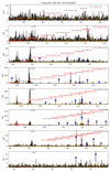 |
Fig. A.1. Normal échelle diagram for KIC 9467102. The frequencies are folded by the large separation Δν = 10.4278 μHz. The modes that are used in the fitting procedure are marked by the colour symbols: green ‘+’ for m = 1, purple ‘•’ for m = 0, and red ‘-’ for m=-1 modes. The best-fitting results are shown by the horizontal red lines, which connect the components in each triplet. We note that the overlap is serious. |
Appendix B: All the diagrams
We show the related diagrams of all the 13 stars. For each star, there are four diagrams shown in the following order: normal échelle diagram, stretched échelle diagram, splitting asymmetry as a function of frequency, and corner diagram of the MCMC fit result.
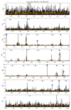 |
Fig. B.1. Normal échelle diagram of KIC 4458118. The frequencies are folded by the large separation Δν = 16.4420 μHz. The modes which are used in the fitting procedure are marked by the colour symbols: green ‘+’ for m = 1, purple ‘•’ for m = 0, and red ‘-’ for m=-1 modes. The best-fitting frequencies are marked by the black ‘+’, ‘•’, ‘-’ symbols at the top of each panel. |
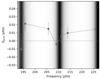 |
Fig. B.3. Splitting asymmetries as a function of frequency of KIC 4458118. Symbols are explained in Fig. 4. |
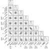 |
Fig. B.4. Corner diagram of the MCMC fitting result of KIC 4458118. |
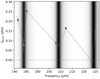 |
Fig. B.7. Splitting asymmetries as a function of frequency of KIC 5196300. Symbols are explained in Fig. 4. |
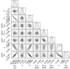 |
Fig. B.8. Corner diagram of the MCMC fitting result of KIC 5196300. |
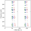 |
Fig. B.10. Stretched échelle diagram of KIC 5696081. Symbols are explained in Fig. 1. |
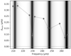 |
Fig. B.11. Splitting asymmetries as a function of frequency of KIC 5696081. Symbols are explained in Fig. 4. |
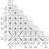 |
Fig. B.12. Corner diagram of the MCMC fitting result of KIC 5696081. |
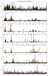 |
Fig. B.13. Normal échelle diagram of KIC 6936091. See Fig. B.1 for the explanations of the symbols. |
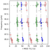 |
Fig. B.14. Stretched échelle diagram of KIC 6936091. Symbols are explained in Fig. 1. |
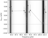 |
Fig. B.15. Splitting asymmetries as a function of frequency of KIC 6936091. Symbols are explained in Fig. 4. |
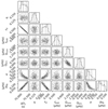 |
Fig. B.16. Corner diagram of the MCMC fitting result of KIC 6936091. |
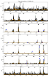 |
Fig. B.17. Normal échelle diagram of KIC 7009365. See Fig. B.1 for the explanations of the symbols. |
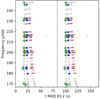 |
Fig. B.18. Stretched échelle diagram of KIC 7009365. Symbols are explained in Fig. 1. |
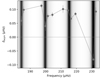 |
Fig. B.19. Splitting asymmetries as a function of frequency of KIC 7009365. Symbols are explained in Fig. 4. |
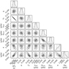 |
Fig. B.20. Corner diagram of the MCMC fitting result of KIC 7009365. |
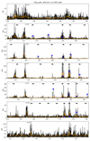 |
Fig. B.21. Normal échelle diagram of KIC 7518143. See Fig. B.1 for the explanations of the symbols. |
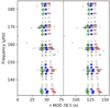 |
Fig. B.22. Stretched échelle diagram of KIC 7518143. Symbols are explained in Fig. 1. |
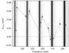 |
Fig. B.23. Splitting asymmetries as a function of frequency of KIC 7518143. Symbols are explained in Fig. 4. |
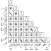 |
Fig. B.24. Corner diagram of the MCMC fitting result of KIC 7518143. |
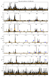 |
Fig. B.25. Normal échelle diagram of KIC 8540034. See Fig. B.1 for the explanations of the symbols. |
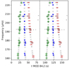 |
Fig. B.26. Stretched échelle diagram of KIC 8540034. Symbols are explained in Fig. 1. |
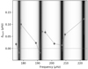 |
Fig. B.27. Splitting asymmetries as a function of frequency of KIC 8540034. Symbols are explained in Fig. 4. |
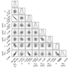 |
Fig. B.28. Corner diagram of the MCMC fitting result of KIC 8540034. |
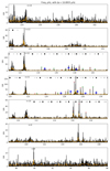 |
Fig. B.29. Normal échelle diagram of KIC 8619145. See Fig. B.1 for the explanations of the symbols. |
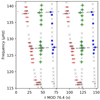 |
Fig. B.30. Stretched échelle diagram of KIC 8619145. Symbols are explained in Fig. 1. |
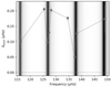 |
Fig. B.31. Splitting asymmetries as a function of frequency of KIC 8619145. Symbols are explained in Fig. 4. |
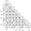 |
Fig. B.32. Corner diagram of the MCMC fitting result of KIC 8619145. |
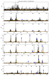 |
Fig. B.33. Normal échelle diagram of KIC 8684542. See Fig. B.1 for the explanations of the symbols. |
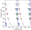 |
Fig. B.34. Stretched échelle diagram of KIC 8684542. Symbols are explained in Fig. 1. |
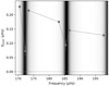 |
Fig. B.35. Splitting asymmetries as a function of frequency of KIC 8684542. Symbols are explained in Fig. 4. |
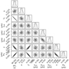 |
Fig. B.36. Corner diagram of the MCMC fitting result of KIC 8684542. |
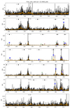 |
Fig. B.37. Normal échelle diagram of KIC 9202471. See Fig. B.1 for the explanations of the symbols. |
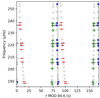 |
Fig. B.38. Stretched échelle diagram of KIC 9202471. Symbols are explained in Fig. 1. |
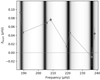 |
Fig. B.39. Splitting asymmetries as a function of frequency of KIC 9202471. Symbols are explained in Fig. 4. |
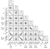 |
Fig. B.40. Corner diagram of the MCMC fitting result of KIC 9202471. |
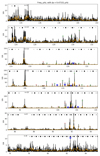 |
Fig. B.41. Normal échelle diagram of KIC 9589420. See Fig. B.1 for the explanations of the symbols. |
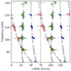 |
Fig. B.42. Stretched échelle diagram of KIC 9589420. Symbols are explained in Fig. 1. |
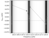 |
Fig. B.43. Splitting asymmetries as a function of frequency of KIC 9589420. Symbols are explained in Fig. 4. |
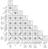 |
Fig. B.44. Corner diagram of the MCMC fitting result of KIC 9589420. |
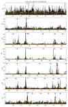 |
Fig. B.45. Normal échelle diagram of KIC 10801792. See Fig. B.1 for the explanations of the symbols. |
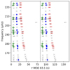 |
Fig. B.46. Stretched échelle diagram of KIC 10801792. Symbols are explained in Fig. 1. |
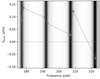 |
Fig. B.47. Splitting asymmetries as a function of frequency of KIC 10801792. Symbols are explained in Fig. 4. |
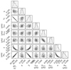 |
Fig. B.48. Corner diagram of the MCMC fitting result of KIC 10801792. |
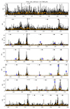 |
Fig. B.49. Normal échelle diagram of KIC 11515377. See Fig. B.1 for the explanations of the symbols. |
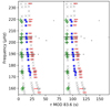 |
Fig. B.50. Stretched échelle diagram of KIC 11515377. Symbols are explained in Fig. 1. |
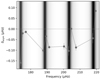 |
Fig. B.51. Splitting asymmetries as a function of frequency of KIC 11515377. Symbols are explained in Fig. 4. |
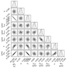 |
Fig. B.52. Corner diagram of the MCMC fitting result of KIC 11515377. |
Appendix C: Other parameters
C.1. Δν vs ΔΠ1
Figure C.1 displays the correlation between the measured period spacing ΔΠ1 and the frequency separation Δν. The frequency separations are distributed between ∼8 to ∼18 μHz and the period spacings range from ∼75 to ∼90 s. All the stars are located at the well-defined ΔΠ1–Δν degenerate ridge, as shown by the grey dots by Mosser et al. (2018), which implies that these stars did not undergo any mass transfer or binary merger (e.g. Deheuvels et al. 2022; Rui & Fuller 2021). We find that our stars tend to locate close to the lower boundary of the ΔΠ1–Δν ridge, implying that they have higher masses (Deheuvels et al. 2022).
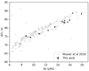 |
Fig. C.1. The correlation between Δν and ΔΠ1. The grey circles are given by Mosser et al. (2018). |
C.2. q, εg, and fshift
We show the values of the coupling factor q in Fig. C.2. The q values of our stars are in the typical range of red giant stars, and we also reproduce the increasing trend between q and ΔΠ1 (e.g. Mosser et al. 2018).
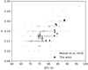 |
Fig. C.2. The coupling factor q vs ΔΠ1. The grey circles are reported by Mosser et al. (2018). |
The g-mode phases εg are displayed in Fig. C.3. We only applied a uniform prior for εg, but we still find that most of the stars have the typical εg values of red giant stars, which is 0.28 ± 0.08 reported by both observations (Mosser et al. 2018) and theoretical predictions that do not include magnetic perturbations (Takata 2016). Therefore, the magnetism-induced perturbation does not affect the distribution of g-mode phase. KIC 8619145 has a large εg with large uncertainty, and we cannot provide strong constraint on εg of KIC 6936091 either.
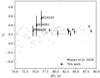 |
Fig. C.3. The g-mode phase εg as a function of ΔΠ1. |
The frequency correction of l = 1 pure p modes fshift in Eq. 4 is a new parameter that has not been studied in previous work. We plot fshift as function of Δν in Fig. C.4. The best values of fshift lie between ∼0.5 to ∼0.75 μHz. It seems that there is a rapid drop when Δν ≲ 10 μHz, but this feature needs more stars to confirm.
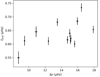 |
Fig. C.4. fshift as a function of Δν. |
Appendix D: Linear relation between ℐ and ΔΠ1
Using the best-fitting models, we calculated the core factors ℐ and derived the field strengths, listed in Table 5. The core factor ℐ is vital to calculate the field strength in Eq. 19, but it is time-consuming to run a stellar evolution code to derive it. Hence, we report an empirical relation between ℐ and the period spacing ΔΠ1. As shown in Fig. D.1, there is a linear relation between ℐ and ΔΠ1, which is characterised as
 (D.1)
(D.1)
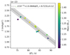 |
Fig. D.1. The core factor ℐ as a function of ΔΠ1, colour coded by the model-inferred masses. The grey dashed line shows the linear fit and the shaded area gives the 1σ range. |
All Tables
Values and their uncertaintiers of Teff, log L/L⊙, and [Fe/H] that were used to constrain the theoretical models.
All Figures
|
Fig. 1. Stretched échelle diagram of KIC 5792889 that does not show any magnetism-induced perturbation. The x-axis is the stretched periods τ modulo ΔΠ1 ≈ 81.6 s. The peaks with S/N > 10 are shown by the grey points (l = 0 and l = 2 modes have been removed). The green ‘+’ stands for the m = 1 modes. The red ‘−’ stands for the m = −1 modes. The blue ‘•’ shows the m = 0 modes. The best-fitting results are plotted by the cross. |
| In the text | |
|
Fig. 2. Stretched échelle diagram of KIC 9467102, which does not show any magnetism-induced perturbation. The symbols are the same as Fig. 1. We show this star as an example because its splittings overlap seriously. |
| In the text | |
|
Fig. 3. Three continuous asymmetric splittings in KIC 5696081. The top and bottom panels show g-dominated modes while the middle panel displays a p-dominated one. The x-axes of three panels are aligned by the m = 1 and −1 mode frequencies. |
| In the text | |
|
Fig. 4. Asymmetries as a function of frequency in KIC 5696081. The dark fringes show where the p-dominated modes are, while the white background shows the locations of g-dominated modes. |
| In the text | |
|
Fig. 5. Corner diagram of the magnetic fitting of KIC 5696081. The vertical dashed lines mark the median values and ±1σ ranges. |
| In the text | |
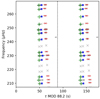 |
Fig. 6. Same as Fig. 1 but for KIC 5696081. This star shows clear asymmetries by magnetic field. |
| In the text | |
|
Fig. 7. Result comparison between this work and Li et al. (2022a). Top panel: measured field strengths by this work and by Li et al. (2022a). Bottom: the ratio between the measured field strengths and the critical strengths. The dotted lines show 1:1 relations. The value of the field strength of KIC 7518143 reported by Li et al. (2022a) is smaller than 41 kG, while we use the median here (20.5 kG). |
| In the text | |
|
Fig. 8. Relation between the asymmetry parameter a and the magnetic shift δνg. KIC 11515377 is the only star that shows negative asymmetries. |
| In the text | |
|
Fig. 9. Relation between the asymmetry parameter a and the field strength. |
| In the text | |
|
Fig. 10. The core rotation rates Ωg as a function of ΔΠ1. The black dots are the stars in this work, and the grey circles are reported by Gehan et al. (2018). |
| In the text | |
|
Fig. 11. Top panel: surface rotation rates as a function of model-inferred radii. Bottom panel: variations in the ratio Ωcore/Ωenv with stellar radii. |
| In the text | |
|
Fig. 12. Field strength as a function of mixed mode density. The red hexagons with errorbars are the field strengths of the 13 stars reported by this work, and the black dots are their critical field strengths. The grey vertical arrows show the lower limits of the field strengths reported by Deheuvels et al. (2023), where the stars do not show any asymmetric splittings, but only m = 0 curved ridges in their stretched échelle diagrams. |
| In the text | |
|
Fig. 13. Top panel: field strengths with model-inferred ages. Bottom panel: field strengths but with model-inferred masses. |
| In the text | |
|
Fig. 14. Ratio of the Alfvèn frequency |
| In the text | |
|
Fig. A.1. Normal échelle diagram for KIC 9467102. The frequencies are folded by the large separation Δν = 10.4278 μHz. The modes that are used in the fitting procedure are marked by the colour symbols: green ‘+’ for m = 1, purple ‘•’ for m = 0, and red ‘-’ for m=-1 modes. The best-fitting results are shown by the horizontal red lines, which connect the components in each triplet. We note that the overlap is serious. |
| In the text | |
|
Fig. B.1. Normal échelle diagram of KIC 4458118. The frequencies are folded by the large separation Δν = 16.4420 μHz. The modes which are used in the fitting procedure are marked by the colour symbols: green ‘+’ for m = 1, purple ‘•’ for m = 0, and red ‘-’ for m=-1 modes. The best-fitting frequencies are marked by the black ‘+’, ‘•’, ‘-’ symbols at the top of each panel. |
| In the text | |
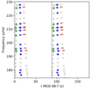 |
Fig. B.2. Stretched échelle diagram of KIC 4458118. Symbols are explained in Fig. 1. |
| In the text | |
|
Fig. B.3. Splitting asymmetries as a function of frequency of KIC 4458118. Symbols are explained in Fig. 4. |
| In the text | |
|
Fig. B.4. Corner diagram of the MCMC fitting result of KIC 4458118. |
| In the text | |
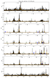 |
Fig. B.5. Normal échelle diagram of KIC 5196300. See Fig. B.1 for the explanations of the symbols. |
| In the text | |
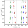 |
Fig. B.6. Stretched échelle diagram of KIC 5196300. Symbols are explained in Fig. 1. |
| In the text | |
|
Fig. B.7. Splitting asymmetries as a function of frequency of KIC 5196300. Symbols are explained in Fig. 4. |
| In the text | |
|
Fig. B.8. Corner diagram of the MCMC fitting result of KIC 5196300. |
| In the text | |
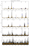 |
Fig. B.9. Normal échelle diagram of KIC 5696081. See Fig. B.1 for the explanations of the symbols. |
| In the text | |
|
Fig. B.10. Stretched échelle diagram of KIC 5696081. Symbols are explained in Fig. 1. |
| In the text | |
|
Fig. B.11. Splitting asymmetries as a function of frequency of KIC 5696081. Symbols are explained in Fig. 4. |
| In the text | |
|
Fig. B.12. Corner diagram of the MCMC fitting result of KIC 5696081. |
| In the text | |
|
Fig. B.13. Normal échelle diagram of KIC 6936091. See Fig. B.1 for the explanations of the symbols. |
| In the text | |
|
Fig. B.14. Stretched échelle diagram of KIC 6936091. Symbols are explained in Fig. 1. |
| In the text | |
|
Fig. B.15. Splitting asymmetries as a function of frequency of KIC 6936091. Symbols are explained in Fig. 4. |
| In the text | |
|
Fig. B.16. Corner diagram of the MCMC fitting result of KIC 6936091. |
| In the text | |
|
Fig. B.17. Normal échelle diagram of KIC 7009365. See Fig. B.1 for the explanations of the symbols. |
| In the text | |
|
Fig. B.18. Stretched échelle diagram of KIC 7009365. Symbols are explained in Fig. 1. |
| In the text | |
|
Fig. B.19. Splitting asymmetries as a function of frequency of KIC 7009365. Symbols are explained in Fig. 4. |
| In the text | |
|
Fig. B.20. Corner diagram of the MCMC fitting result of KIC 7009365. |
| In the text | |
|
Fig. B.21. Normal échelle diagram of KIC 7518143. See Fig. B.1 for the explanations of the symbols. |
| In the text | |
|
Fig. B.22. Stretched échelle diagram of KIC 7518143. Symbols are explained in Fig. 1. |
| In the text | |
|
Fig. B.23. Splitting asymmetries as a function of frequency of KIC 7518143. Symbols are explained in Fig. 4. |
| In the text | |
|
Fig. B.24. Corner diagram of the MCMC fitting result of KIC 7518143. |
| In the text | |
|
Fig. B.25. Normal échelle diagram of KIC 8540034. See Fig. B.1 for the explanations of the symbols. |
| In the text | |
|
Fig. B.26. Stretched échelle diagram of KIC 8540034. Symbols are explained in Fig. 1. |
| In the text | |
|
Fig. B.27. Splitting asymmetries as a function of frequency of KIC 8540034. Symbols are explained in Fig. 4. |
| In the text | |
|
Fig. B.28. Corner diagram of the MCMC fitting result of KIC 8540034. |
| In the text | |
|
Fig. B.29. Normal échelle diagram of KIC 8619145. See Fig. B.1 for the explanations of the symbols. |
| In the text | |
|
Fig. B.30. Stretched échelle diagram of KIC 8619145. Symbols are explained in Fig. 1. |
| In the text | |
|
Fig. B.31. Splitting asymmetries as a function of frequency of KIC 8619145. Symbols are explained in Fig. 4. |
| In the text | |
|
Fig. B.32. Corner diagram of the MCMC fitting result of KIC 8619145. |
| In the text | |
|
Fig. B.33. Normal échelle diagram of KIC 8684542. See Fig. B.1 for the explanations of the symbols. |
| In the text | |
|
Fig. B.34. Stretched échelle diagram of KIC 8684542. Symbols are explained in Fig. 1. |
| In the text | |
|
Fig. B.35. Splitting asymmetries as a function of frequency of KIC 8684542. Symbols are explained in Fig. 4. |
| In the text | |
|
Fig. B.36. Corner diagram of the MCMC fitting result of KIC 8684542. |
| In the text | |
|
Fig. B.37. Normal échelle diagram of KIC 9202471. See Fig. B.1 for the explanations of the symbols. |
| In the text | |
|
Fig. B.38. Stretched échelle diagram of KIC 9202471. Symbols are explained in Fig. 1. |
| In the text | |
|
Fig. B.39. Splitting asymmetries as a function of frequency of KIC 9202471. Symbols are explained in Fig. 4. |
| In the text | |
|
Fig. B.40. Corner diagram of the MCMC fitting result of KIC 9202471. |
| In the text | |
|
Fig. B.41. Normal échelle diagram of KIC 9589420. See Fig. B.1 for the explanations of the symbols. |
| In the text | |
|
Fig. B.42. Stretched échelle diagram of KIC 9589420. Symbols are explained in Fig. 1. |
| In the text | |
|
Fig. B.43. Splitting asymmetries as a function of frequency of KIC 9589420. Symbols are explained in Fig. 4. |
| In the text | |
|
Fig. B.44. Corner diagram of the MCMC fitting result of KIC 9589420. |
| In the text | |
|
Fig. B.45. Normal échelle diagram of KIC 10801792. See Fig. B.1 for the explanations of the symbols. |
| In the text | |
|
Fig. B.46. Stretched échelle diagram of KIC 10801792. Symbols are explained in Fig. 1. |
| In the text | |
|
Fig. B.47. Splitting asymmetries as a function of frequency of KIC 10801792. Symbols are explained in Fig. 4. |
| In the text | |
|
Fig. B.48. Corner diagram of the MCMC fitting result of KIC 10801792. |
| In the text | |
|
Fig. B.49. Normal échelle diagram of KIC 11515377. See Fig. B.1 for the explanations of the symbols. |
| In the text | |
|
Fig. B.50. Stretched échelle diagram of KIC 11515377. Symbols are explained in Fig. 1. |
| In the text | |
|
Fig. B.51. Splitting asymmetries as a function of frequency of KIC 11515377. Symbols are explained in Fig. 4. |
| In the text | |
|
Fig. B.52. Corner diagram of the MCMC fitting result of KIC 11515377. |
| In the text | |
|
Fig. C.1. The correlation between Δν and ΔΠ1. The grey circles are given by Mosser et al. (2018). |
| In the text | |
|
Fig. C.2. The coupling factor q vs ΔΠ1. The grey circles are reported by Mosser et al. (2018). |
| In the text | |
|
Fig. C.3. The g-mode phase εg as a function of ΔΠ1. |
| In the text | |
|
Fig. C.4. fshift as a function of Δν. |
| In the text | |
|
Fig. D.1. The core factor ℐ as a function of ΔΠ1, colour coded by the model-inferred masses. The grey dashed line shows the linear fit and the shaded area gives the 1σ range. |
| In the text | |
Current usage metrics show cumulative count of Article Views (full-text article views including HTML views, PDF and ePub downloads, according to the available data) and Abstracts Views on Vision4Press platform.
Data correspond to usage on the plateform after 2015. The current usage metrics is available 48-96 hours after online publication and is updated daily on week days.
Initial download of the metrics may take a while.