| Issue |
A&A
Volume 670, February 2023
|
|
|---|---|---|
| Article Number | L16 | |
| Number of page(s) | 9 | |
| Section | Letters to the Editor | |
| DOI | https://doi.org/10.1051/0004-6361/202245282 | |
| Published online | 09 February 2023 | |
Letter to the Editor
Strong magnetic fields detected in the cores of 11 red giant stars using gravity-mode period spacings
IRAP, Université de Toulouse, CNRS, CNES, UPS, 14 avenue Edouard Belin, 31400 Toulouse, France
e-mail: This email address is being protected from spambots. You need JavaScript enabled to view it.
Received:
24
October
2022
Accepted:
3
January
2023
Abstract
Despite their importance in stellar evolution, little is known about magnetic fields in the interior of stars. The recent seismic detection of magnetic fields in the core of several red giant stars has given measurements of their strength and information on their topology. We revisit the puzzling case of hydrogen-shell burning giants that show deviations from the expected regular period spacing of gravity modes. These stars also tend to have a measured period spacing that is too low compared to their counterparts. In this Letter, we show that these two features are well accounted for by strong magnetic fields in the cores of these stars. For 11 Kepler red giants showing these anomalies, we placed lower limits on the core field strengths ranging from 40 to 610 kG. For one star, the measured field exceeds the critical field above which gravity waves no longer propagate in the core. We find that this star shows mixed mode suppression at low frequency, which further suggests that this phenomenon might be related to strong core magnetic fields.
Key words: asteroseismology / stars: magnetic field
© The Authors 2023
 Open Access article, published by EDP Sciences, under the terms of the Creative Commons Attribution License (https://creativecommons.org/licenses/by/4.0), which permits unrestricted use, distribution, and reproduction in any medium, provided the original work is properly cited.
This article is published in open access under the Subscribe-to-Open model. This email address is being protected from spambots. You need JavaScript enabled to view it. to support open access publication.
1. Introduction
Magnetic fields affect stars at all evolutionary stages from star-forming molecular clouds to white dwarfs and magnetars (McKee & Ostriker 2007; Kaspi & Beloborodov 2017; Ferrario et al. 2020). In particular, they are expected to play a central role in the redistribution of angular momentum inside stars (Maeder & Meynet 2005; Cantiello et al. 2014; Rüdiger et al. 2015), and thus in the transport of chemical elements. While surface magnetic fields have been detected and characterized in stars across the Hertzsprung–Russell diagram (Landstreet 1992; Donati & Landstreet 2009), internal magnetic fields have long remained inaccessible to direct observations. In red giant stars, the detection of mixed modes – that is, oscillation modes that behave as gravity (g) modes in the core and as pressure modes in the envelope – has given strong evidence that the cores of red giant stars are rotating slowly (e.g., Deheuvels et al. 2012; Mosser et al. 2012b; Gehan et al. 2018). This has yielded evidence that angular momentum is redistributed much more efficiently than if only purely hydrodynamical processes were at work (e.g., Marques et al. 2013). Magnetic fields could produce the additional transport that is needed (Rüdiger et al. 2015; Jouve et al. 2015; Fuller et al. 2019; Petitdemange et al. 2023). Observational constraints on the properties of internal magnetic fields are crucially needed to assess the nature and the efficiency of the magnetic transport of angular momentum inside stars.
The propagation of magneto-gravity waves is expected to be suppressed when the magnetic field exceeds a critical strength Bc above which Alfvén wave frequencies become comparable to those of gravity waves. This phenomenon was invoked by Fuller et al. (2015) to account for the unexpectedly low amplitudes of dipole mixed modes in a fraction of red giants (see also Mosser et al. 2012a; Stello et al. 2016). For core fields above Bc, Fuller et al. (2015) suggest that the mode energy reaching the magnetized core would be entirely dissipated and lost, giving rise to purely p-like dipole modes. This interpretation has been questioned by Mosser et al. (2017), who found that partially suppressed dipole modes still retain a g-like character. Loi (2020b) later showed that even with strong fields, a fraction of the incoming waves could remain g-like, which would allow for partial energy to return from the core. The interpretation of suppressed dipole modes remains debated.
Magnetic fields also produce shifts in the oscillation mode frequencies (Gough 1990). Several studies have recently investigated the impact of internal fields on the frequencies of mixed modes in red giants (Gomes & Lopes 2020; Bugnet et al. 2021; Loi 2021). Very recently, Li et al. (2022) detected clear asymmetries in the rotational multiplets of dipole mixed modes in three Kepler red giants. They show that these features can only be accounted for by internal magnetic fields with intensities ranging from 30 to 130 kG in the vicinity of the hydrogen burning shell. These findings have made it possible to characterize magnetic fields in the cores of red giants.
In this Letter, we investigate the irregularity of g-mode period spacings in a group of red giant branch (RGB) stars, which thus far remains unexplained. High-radial-order g modes are expected to be approximately equally spaced in period by ΔΠl, where l is the mode degree. In red giants, dipole mixed modes can be used to measure ΔΠ1 using asymptotic expressions of the mode frequencies (Mosser et al. 2015). While ΔΠ1 is nearly constant over the frequency range of observed modes for the vast majority of RGB stars, some red giants show significant variations of ΔΠ1 (Mosser et al. 2018; Deheuvels et al. 2022). Here, we show that this feature is the signature of strong magnetic fields in the cores of these stars. This constitutes a new way of detecting and characterizing magnetic fields in the cores of red giants.
In Sect. 2, we present red giants that exhibit deviations from the regular period spacing pattern of g modes, and we find additional such targets in Kepler data. We then show in Sect. 3 that strong core magnetic fields can account for this phenomenon. In Sect. 4, we determine the field strengths that are required to match the seismic observations. We discuss these measurements in Sect. 5, before concluding in Sect. 6.
2. Red giants with nonconstant ΔΠ1
2.1. Previous detections of nonconstant ΔΠ1 in RGB stars
To first order, high-radial-order gravity modes are expected to be equally spaced in period. Among the 160 RGB stars studied by Mosser et al. (2018), only one shows clear deviations from a regular period spacing of g modes (KIC 3216736). The authors attribute this irregularity to a buoyancy glitch (that is, a sharp variation in the Brunt–Väisälä frequency N), which induces periodic variations in the asymptotic period spacing ΔΠ1.
More recently, Deheuvels et al. (2022) identified additional RGB stars with nonconstant ΔΠ1, in a different context. These stars appeared among a peculiar class of RGB stars that are located below the so-called degeneracy sequence in the (Δν, ΔΠ1) plane, where RGB stars regroup when electron degeneracy becomes strong in their core. Most of the stars in this class are intermediate-mass stars and are thought to result from mass transfer (Deheuvels et al. 2022). The only four lower-mass stars with ΔΠ1 being too low must have a different origin. Contrary to intermediate-mass stars, they all show clear departures from a constant period spacing of g modes. Interestingly, the star identified by Mosser et al. (2018; KIC 3216736) is among these targets. This suggests that there might be a link between the nonconstancy of ΔΠ1 and the fact that its measured value is abnormally low. These four stars show only one detected mode per rotational multiplet.
2.2. Additional targets
We searched for other targets showing nonconstant ΔΠ1 among RGB stars with detected oscillations using the catalog of Yu et al. (2018). To estimate the period spacings of g modes using dipole mixed modes, we computed the so-called stretched periods τ, defined by the differential equation dτ = dP/ζ (Mosser et al. 2015), where ζ corresponds to the fraction of the mode kinetic energy that is enclosed in the g-mode cavity (ζ tends to 1 for pure g modes, and 0 for pure p modes). When building échelle diagrams of these stretched periods, mixed modes are expected to align in a vertical ridge if ΔΠ1 is constant and deviations from a regular period spacing induce curvature in this ridge.
We searched for stars with only one curved ridge detected in order to avoid the additional complication coming from rotational effects (these effects will be addressed in a subsequent work). This can mean that these stars are seen pole-on, so that only the m = 0 modes can be detected. This could also arise if the core rotation is too weak to produce detectable rotational splitting in Kepler data. We thus found seven additional targets, bringing the total of the sample to 11 stars (see Table B.1). Their stretched period échelle diagrams are shown in Figs. 1 and B.1. They were folded using an average value of the asymptotic period spacing over the frequency range of the observations, which is further referred to as  .
.
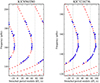 |
Fig. 1. Stretched period échelle diagrams of two red giants showing distortion from the regular g-mode pattern. Blue circles show detected dipole modes. Red crosses correspond to the best-fit asymptotic mixed mode frequencies obtained by including a magnetic perturbation. |
The location of these 11 targets in the (Δν, ΔΠ1) plane is shown in Fig. 2 (black star symbols), where we have used the values  as the measured asymptotic period spacing. Three of the seven additional targets lie well below the degeneracy sequence of RGB stars, which confirms the link between nonconstant ΔΠ1 and low measured values for these quantities.
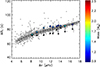 |
Fig. 2. Location of RGB stars with nonconstant ΔΠ1 in the (Δν, ΔΠ1) plane. Black star symbols correspond to the values of ΔΠ1 that produce the best vertical alignment of modes in the stretched period échelle diagram (Sect. 2). Colored star symbols correspond to the corrected values of ΔΠ1 obtained by taking into account the magnetic perturbation to the mode frequencies (Sect. 4). Other RGB stars from Vrard et al. (2016) are shown as gray circles (for clarity, stars flagged by the authors as potential aliases were omitted). |
2.3. Origin of the observed distortions in the g-mode pattern
Deviations from a regular ΔΠ1 are generally attributed to buoyancy glitches (e.g., Mosser et al. 2015). To produce the observed distortions in ΔΠ1, we show in Appendix A that a buoyancy glitch needs to have a large amplitude (the local value of N must be multiplied by a factor of at least six) and be located either deep inside the inert He core, or well above the H-burning shell. While this cannot be excluded, no known process is expected to produce such strong features in these regions of an RGB star. Secondly, the shape of the modulation in ΔΠ1 that is produced by a large-amplitude glitch strongly differs from the observations (see Appendix A). Finally, the hypothesis of a buoyancy glitch would not explain why the measured values of ΔΠ1 are unexpectedly low for most of our stars. It thus seems unlikely that the observed deviations in ΔΠ1 arise from buoyancy glitches. In the following sections, we explore the possibility that the irregularities in ΔΠ1 are produced by internal magnetic fields.
3. Effects of magnetic fields on g-mode period spacings
The influence of magnetic fields over oscillation mode frequencies has been studied over the last decades using a perturbative approach (Unno et al. 1989; Gough 1990). Recently, their effects on mixed modes in red giants have been addressed in the special case of dipolar fields with specific radial profiles, which are either aligned with the rotation axis (Hasan et al. 2005; Gomes & Lopes 2020; Mathis et al. 2021; Bugnet et al. 2021) or inclined (Loi 2021).
Li et al. (2022) extended these studies to an arbitrary magnetic field and obtained a general expression for the magnetic frequency shift that is valid provided that the azimuthal component is not much larger than the radial one (Bϕ/Br ≪ ωmax/N, where ωmax is the angular frequency at the maximum power of oscillations and N is the Brunt–Väisälä frequency1). Accordingly, the multiplets of l = 1 pure g modes (that is, g modes that are not coupled to p modes) undergo an average shift ωB, given by
 (1)
(1)
where K(r) is a weight function that probes the g-mode cavity and sharply peaks in the vicinity of the H-burning shell (HBS), ℐ is a factor that depends on the core structure (see Eq. (45) and (46) of Li et al. 2022), and  . The angular frequency shifts of the components of g-mode dipole multiplets are then given by
 (2)
(2)
 (3)
(3)
where a is a dimensionless coefficient that depends on the horizontal geometry of  (
( , where P2(cos θ) is the second order Legendre polynomial).
The dependency of magnetic shifts with ω−3 shows that low-frequency (that is, high-radial-order) g modes are more affected by magnetic fields. For this reason, magnetic shifts create a deviation from the regular period spacing of pure g modes, as was already pointed out by Loi (2020a), Bugnet et al. (2021), and Li et al. (2022). Very recently Bugnet (2022) proposed a method to detect the signature of magnetic fields exploiting this property.
For illustration purposes, Fig. 1 shows stretched échelle diagrams of mixed modes with magnetic perturbations (see Sect. 4). The left panel corresponds to a case where the unperturbed g modes have an asymptotic period spacing of ΔΠ1 = 85 s, and we have added a magnetic perturbation corresponding to a frequency shift of 3.9 μHz at νmax. The ridge appears strongly curved, similarly to the observations. To visualize the ridge properly, the stretched échelle diagram was folded using a period spacing of  = 73.8 s, which is much lower than the unperturbed period spacing ΔΠ1.
Magnetic perturbations thus account for both characteristics of the stars identified in Sect. 2. First, they produce curved ridges in the period échelle diagram. Since magnetic shifts are always positive, the period spacings of g modes decrease with decreasing mode frequency. Thus, the curvature always has the same shape, with the low-frequency part of the ridge being bent to the left of the period échelle diagram. Interestingly, all the targets identified in Sect. 2 show ridges that are curved in this direction (see Fig. B.1). Secondly, magnetic perturbations yield a measured period spacing that is significantly lower than the asymptotic unperturbed period spacing ΔΠ1. This can explain why most of the targets identified in Sect. 2 are located below the degenerate sequence in the (Δν, ΔΠ1) plane.
4. Measurement of magnetic field strengths
We then estimated the field strengths that are required to account for the observations. For this purpose, we computed asymptotic expressions of the mixed mode frequencies including magnetic perturbations. We followed the method that we propose in Li et al. (2022), which is briefly recalled here. The effects of magnetic fields are taken into account by adding a magnetic perturbation to the frequencies of pure p and g modes. These perturbed frequencies are then plugged into the asymptotic expression of mixed mode frequencies given by Shibahashi (1979). While the frequencies of p modes are unaffected (Li et al. 2022), the periods of g modes are expressed as
 (4)
(4)
where Pg, 0 = (ng + 1/2 + εg)ΔΠ1 is the first-order asymptotic expression of l = 1 g modes without a perturbation, and δωg is the magnetic perturbation to g-mode frequencies. Using Eqs. (1)–(3), δωg can be written as δωg = δω0(ωmax/ω)3, where δω0 corresponds to the magnetic shift at ωmax.
For the 11 stars of our sample, we optimized the values of ΔΠ1, δω0, εg, and d01 (defined below) to match the observations as best as possible using a Markov chain Monte Carlo approach. Based on the measurements of εg for hundreds of Kepler red giants by Mosser et al. (2018), we assumed a Gaussian prior on εg with a mean of 0.28 and a standard deviation of 0.08, and we considered uniform priors for the other parameters. The characteristics of pure p modes were derived from the observed radial modes, with the exception of d01, defined as the average small separation νp, l = 0 − νp, l = 1 + Δν/2, which was considered as a free parameter of the fit.
The optimal parameters of the fit are given in Table B.1. The corresponding asymptotic frequencies are shown as red crosses in Figs. 1 and B.1. The agreement with the observations is very good, with the curvature of the ridge being well reproduced for all the stars. The fit also provides an estimate of the unperturbed asymptotic period spacing ΔΠ1 for these stars, which is, as expected, larger than the apparent period spacing  . We used the newly determined values of ΔΠ1 to update the location of the 11 targets in the (Δν, ΔΠ1) plane in Fig. 2 (colored star symbols). It is striking to observe that they now lie on the degenerate sequence, as expected for stars in this mass range and evolutionary state. Thus, there is a body of evidence that the distortions to the g-mode pattern that are observed in the 11 targets of the sample are indeed produced by internal magnetic fields. This yields the opportunity to characterize these fields.
The measurement of δω0 can be used to derive an estimate of  using Eqs. (1)–(3). The obtained expression depends on the asymmetry parameter a, which can unfortunately not be measured with only one component detected per multiplet. However, we have shown that −1/2 ≤ a ≤ 1 (Li et al. 2022), so that we could place a lower limit on the value of
  . We obtain
 (5)
(5)
where μ0 is the magnetic permeability. This expression is valid regardless of whether the observed modes have an azimuthal number of m = 0 or m = ±1 (indeed, the factors 1 − a and 1 + a/2 appearing in Eq. (2) and (3), respectively, are both always inferior to 3/2). Only in the very specific case of a field that is entirely concentrated on the poles (a → 1) would the measured field be much larger than  . For instance, if
  had an axisymmetric dipolar configuration (a = 2/5), we would have
  .
.
To calculate  , the term ℐ must be known, for which a model of the stellar internal structure is needed. For this purpose, we used a precomputed grid of stellar models of red giants with various masses, metallicities, and evolutionary stages, built with the evolution code MESA (Paxton et al. 2011). For each target, we selected models from the grid that simultaneously reproduce the asymptotic large separation of p modes Δν and the asymptotic period spacing of dipole g modes ΔΠ1. The models that satisfy this condition all give similar estimates of ℐ. We thus obtained measurements of
  ranging from about 40 kG to about 610 kG (see Table B.1).
5. Discussion
5.1. Magnetic field strength versus evolution
In Fig. 3, we plotted the measured field strengths as a function of the density of mixed modes  , which is a good proxy for the evolution along the red giant branch (Gehan et al. 2018). We observe a clear decrease in the measured field intensities along the evolution. At first sight, this trend is surprising. Indeed, assuming conservation of the magnetic flux, the contraction of the core as red giants evolve should increase the field intensity, so that one would have expected the opposite trend. Before interpreting this trend, we address the question of potential observational biases. In Appendix C, we calculate the threshold field strength Bth that is required to produce detectable variations in the g-mode period spacing over the observed frequency range. As shown in Fig. 3, Bth decreases along the evolution on the RGB. This explains why we do not detect lower-intensity fields in unevolved red giants. However, the lack of higher-intensity fields in more evolved stars cannot be explained by this observational bias, and thus the decrease in the field strength with evolution seems real.
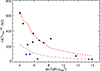 |
Fig. 3. Minimal field strength |

5.2. Comparison with the critical field
We compared the measured minimal field intensities with the critical field Bc. We stress that for fields over Bc, a local analysis shows that gravity waves can no longer propagate (Fuller et al. 2015). While the details of how global modes are affected remain uncertain, it is clear that they will be impacted. We used the stellar models selected from our grid in Sect. 4 to estimate Bc for each star of the sample. We evaluated Bc in the HBS, where it reaches a sharp minimum (Fuller et al. 2015), and where our field measurements have the highest sensitivity. Figure 3 shows that the value of Bc in the HBS decreases with evolution, as has already been pointed out by Fuller et al. (2015). We observe that our minimal field strength measurements closely follow the trend of Bc with evolution. One possible explanation for the trend observed in Fig. 3 is that the core field increases with evolution, owing to magnetic flux conservation, and eventually reaches the critical field Bc. Above this field, mixed modes would no longer form, making the seismic detection of core magnetic fields impossible.
5.3. Link with stars with suppressed dipole mixed modes
The ratio between the minimal measured field strength and the critical field Bc is maximal for KIC 6975038, where it reaches a factor of about 1.7. Interestingly, this star shows clear signs of dipole mixed mode suppression. Figure 4 shows the power spectrum of KIC 6975038 built with Kepler data. The regions of the spectrum where dipole mixed modes are expected are highlighted in red. While the dipole mixed mode pattern clearly appears at high frequency, it is nearly absent for frequencies around νmax and below.
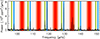 |
Fig. 4. Power spectrum of KIC 6975038 obtained from Kepler data. Color-shaded areas indicate the location of l = 0 (blue), l = 1 (red), and l = 2 (green) modes. |
This type of behavior is expected, assuming that field intensities above the critical field Bc can suppress mixed modes. Indeed, Bc varies as ω2, so that for a given field strength, there exists a transition frequency ωc below which mixed modes should be strongly suppressed and above which they should be unaffected (Fuller et al. 2015; Loi 2020b). This can be used to estimate the field strength for stars where the transition between suppressed and normal modes can be detected, as was proposed by Fuller et al. (2015) for KIC 8561221 (García et al. 2014). For KIC 6975038, the observed transition frequency ωc yields a radial field intensity of about 180 kG in the HBS. This estimate has the same order of magnitude as the minimal field strength  kG that was inferred in an independent way using the perturbations to the g-mode period spacing (Sect. 4). This star thus combines two different features that have been interpreted as potential indications of the presence of core magnetic fields and they both lead to comparable estimates of magnetic field strength. While more stars of this type would be required to draw conclusions, this is a further indication that there might be a link between mixed mode suppression and strong core fields.
5.4. Origin of the detected fields
One possibility is that the detected fields were produced by a dynamo in the convective core during the main sequence. The stars of our sample have masses ranging from 1.11 to 1.56 M⊙ (see Table B.1). Contrary to the three stars studied in Li et al. (2022), the lowest-mass stars likely had a radiative core during most of the main sequence. However, even these stars possessed a small initial convective core at the beginning of the main sequence, owing to the burning of 3He and 12C outside of equilibrium (Deheuvels et al. 2010). With the ohmic diffusion timescale being longer than the evolution timescale (Cantiello et al. 2016), these fields can survive until the red giant phase and relax into stable configurations (Braithwaite & Spruit 2004). By using the stellar models introduced in Sect. 4 and assuming a conservation of the magnetic flux, we estimated the main-sequence field strengths that would be required to produce the detected fields (Appendix D). We found minimal field intensities ranging from 1 to 26 kG inside the main-sequence convective cores. This is in general lower than the radial magnetic field strengths found by the numerical simulation of a convective core (Brun et al. 2005) or order-of-magnitude estimates assuming equipartition with the convective motion kinetic energy (Cantiello et al. 2016). A dedicated study will be necessary to determine whether the measured core fields can be accounted for by this possible origin of the fields, taking into account the diversity of the dynamo-generated fields and the dissipation provoked by their relaxation (Becerra et al. 2022) and potential instabilities (Gouhier et al. 2022) in the post-main-sequence phase.
6. Conclusion
In this Letter, we have revisited the puzzling case of H-shell burning red giants that exhibit strong deviations from the regular period spacing that gravity modes should reach in the high-radial-order limit (Deheuvels et al. 2022). We have shown that this peculiarity is unlikely to be produced by buoyancy glitches and, on the contrary, very well accounted for by strong magnetic fields in the core of these stars. We thus placed lower limits on the strength of the radial field in the vicinity of the H-burning shell, ranging from 40 to 610 kG for the 11 stars of our sample. We have also shown that for one star, the measured field exceeds the critical field Bc above which gravity waves can no longer propagate in the core (Fuller et al. 2015). Interestingly, this star shows mixed mode suppression at low frequency, which further suggests that this phenomenon might be related to strong core magnetic fields, although it should be noted that the mechanisms leading to mode suppression remain uncertain. This study has focused on red giants without signs of rotational splitting, to avoid the additional complication arising from rotational effects. We plan to search more generally for similar behavior in Kepler data in the near future.
The ratio ωmax/N typically exceeds 102 for red giants.
Acknowledgments
We thank the anonymous referee for suggestions that improved the clarity of the manuscript. S.D., J.B. and F.L. acknowledge support from from the project BEAMING ANR-18-CE31-0001 of the French National Research Agency (ANR) and from the Centre National d’Etudes Spatiales (CNES).
References
- Becerra, L., Reisenegger, A., Valdivia, J. A., & Gusakov, M. E. 2022, MNRAS, 511, 732 [NASA ADS] [CrossRef] [Google Scholar]
- Braithwaite, J., & Spruit, H. C. 2004, Nature, 431, 819 [Google Scholar]
- Brun, A. S., Browning, M. K., & Toomre, J. 2005, ApJ, 629, 461 [Google Scholar]
- Bugnet, L. 2022, A&A, 667, A68 [NASA ADS] [CrossRef] [EDP Sciences] [Google Scholar]
- Bugnet, L., Prat, V., Mathis, S., et al. 2021, A&A, 650, A53 [NASA ADS] [CrossRef] [EDP Sciences] [Google Scholar]
- Cantiello, M., Mankovich, C., Bildsten, L., Christensen-Dalsgaard, J., & Paxton, B. 2014, ApJ, 788, 93 [Google Scholar]
- Cantiello, M., Fuller, J., & Bildsten, L. 2016, ApJ, 824, 14 [NASA ADS] [CrossRef] [Google Scholar]
- Cunha, M. S., Stello, D., Avelino, P. P., Christensen-Dalsgaard, J., & Townsend, R. H. D. 2015, ApJ, 805, 127 [NASA ADS] [CrossRef] [Google Scholar]
- Cunha, M. S., Avelino, P. P., Christensen-Dalsgaard, J., et al. 2019, MNRAS, 490, 909 [Google Scholar]
- Deheuvels, S., Michel, E., Goupil, M. J., et al. 2010, A&A, 514, A31 [NASA ADS] [CrossRef] [EDP Sciences] [Google Scholar]
- Deheuvels, S., García, R. A., Chaplin, W. J., et al. 2012, ApJ, 756, 19 [Google Scholar]
- Deheuvels, S., Ballot, J., Gehan, C., & Mosser, B. 2022, A&A, 659, A106 [NASA ADS] [CrossRef] [EDP Sciences] [Google Scholar]
- Donati, J. F., & Landstreet, J. D. 2009, ARA&A, 47, 333 [Google Scholar]
- Ferrario, L., Wickramasinghe, D., & Kawka, A. 2020, AdSpR, 66, 1025 [NASA ADS] [Google Scholar]
- Fuller, J., Cantiello, M., Stello, D., Garcia, R. A., & Bildsten, L. 2015, Science, 350, 423 [Google Scholar]
- Fuller, J., Piro, A. L., & Jermyn, A. S. 2019, MNRAS, 485, 3661 [NASA ADS] [Google Scholar]
- García, R. A., Ceillier, T., Salabert, D., et al. 2014, A&A, 572, A34 [NASA ADS] [CrossRef] [EDP Sciences] [Google Scholar]
- Gehan, C., Mosser, B., Michel, E., Samadi, R., & Kallinger, T. 2018, A&A, 616, A24 [NASA ADS] [CrossRef] [EDP Sciences] [Google Scholar]
- Gomes, P., & Lopes, I. 2020, MNRAS, 496, 620 [NASA ADS] [CrossRef] [Google Scholar]
- Gough, D. O. 1990, in Progress of Seismology of the Sun and Stars, eds. Y. Osaki, & H. Shibahashi (Berlin: Springer Verlag), Lecture Notes in Physics, 367, 283 [Google Scholar]
- Gouhier, B., Jouve, L., & Lignières, F. 2022, A&A, 661, A119 [NASA ADS] [CrossRef] [EDP Sciences] [Google Scholar]
- Hasan, S. S., Zahn, J. P., & Christensen-Dalsgaard, J. 2005, A&A, 444, L29 [NASA ADS] [CrossRef] [EDP Sciences] [Google Scholar]
- Jouve, L., Gastine, T., & Lignières, F. 2015, A&A, 575, A106 [NASA ADS] [CrossRef] [EDP Sciences] [Google Scholar]
- Kaspi, V. M., & Beloborodov, A. M. 2017, ARA&A, 55, 261 [Google Scholar]
- Landstreet, J. D. 1992, A&ARv, 4, 35 [NASA ADS] [CrossRef] [Google Scholar]
- Li, G., Deheuvels, S., Ballot, J., & Lignières, F. 2022, Nature, 610, 43 [NASA ADS] [CrossRef] [Google Scholar]
- Loi, S. T. 2020a, MNRAS, 496, 3829 [Google Scholar]
- Loi, S. T. 2020b, MNRAS, 493, 5726 [CrossRef] [Google Scholar]
- Loi, S. T. 2021, MNRAS, 504, 3711 [NASA ADS] [CrossRef] [Google Scholar]
- Maeder, A., & Meynet, G. 2005, A&A, 440, 1041 [NASA ADS] [CrossRef] [EDP Sciences] [Google Scholar]
- Marques, J. P., Goupil, M. J., Lebreton, Y., et al. 2013, A&A, 549, A74 [NASA ADS] [CrossRef] [EDP Sciences] [Google Scholar]
- Mathis, S., Bugnet, L., Prat, V., et al. 2021, A&A, 647, A122 [EDP Sciences] [Google Scholar]
- McKee, C. F., & Ostriker, E. C. 2007, ARA&A, 45, 565 [Google Scholar]
- Miglio, A., Montalbán, J., Noels, A., & Eggenberger, P. 2008, MNRAS, 386, 1487 [Google Scholar]
- Mosser, B., Elsworth, Y., Hekker, S., et al. 2012a, A&A, 537, A30 [NASA ADS] [CrossRef] [EDP Sciences] [Google Scholar]
- Mosser, B., Goupil, M. J., Belkacem, K., et al. 2012b, A&A, 548, A10 [NASA ADS] [CrossRef] [EDP Sciences] [Google Scholar]
- Mosser, B., Vrard, M., Belkacem, K., Deheuvels, S., & Goupil, M. J. 2015, A&A, 584, A50 [NASA ADS] [CrossRef] [EDP Sciences] [Google Scholar]
- Mosser, B., Pinçon, C., Belkacem, K., Takata, M., & Vrard, M. 2017, A&A, 600, A1 [NASA ADS] [CrossRef] [EDP Sciences] [Google Scholar]
- Mosser, B., Gehan, C., Belkacem, K., et al. 2018, A&A, 618, A109 [NASA ADS] [CrossRef] [EDP Sciences] [Google Scholar]
- Paxton, B., Bildsten, L., Dotter, A., et al. 2011, ApJS, 192, 3 [Google Scholar]
- Petitdemange, L., Marcotte, F., & Gissinger, C. 2023, Science, 379 [Google Scholar]
- Rüdiger, G., Gellert, M., Spada, F., & Tereshin, I. 2015, A&A, 573, A80 [NASA ADS] [CrossRef] [EDP Sciences] [Google Scholar]
- Shibahashi, H. 1979, PASJ, 31, 87 [NASA ADS] [Google Scholar]
- Stello, D., Cantiello, M., Fuller, J., et al. 2016, Nature, 529, 364 [Google Scholar]
- Unno, W., Osaki, Y., Ando, H., Saio, H., & Shibahashi, H. 1989, Nonradial Oscillations of Stars (Tokyo: University of Tokyo Press) [Google Scholar]
- Vrard, M., Mosser, B., & Samadi, R. 2016, A&A, 588, A87 [CrossRef] [EDP Sciences] [Google Scholar]
- Yu, J., Huber, D., Bedding, T. R., et al. 2018, ApJS, 236, 42 [NASA ADS] [CrossRef] [Google Scholar]
Appendix A: Role of buoyancy glitches in deviations from constant ΔΠ1
It is well known that buoyancy glitches induce deviations in the pattern of high-radial-order g modes (e.g., Miglio et al. 2008). Such deviations were already found by exploiting the mixed modes of core-helium burning giants (Mosser et al. 2015). Cunha et al. (2015) and Cunha et al. (2019) provide the appropriate formalism to determine the properties of buoyancy glitches (location and amplitude) from their seismic signature. Here, we investigate what types of glitches could produce the strong deviations in the period spacings of g modes that we observed in our sample of Kepler red giants.
A buoyancy glitch produces a periodic modulation in the period spacings of g modes. The period of this modulation is directly related to the position of the glitch. This position is generally expressed in terms of its buoyancy radius or depth. Following the notations of Cunha et al. (2019), the buoyancy radius  and depth
  at a radius r are defined as
 (A.1)
(A.1)
respectively, where L = [l(l + 1)]1/2, and r1 and r2 are the inner and outer turning points of the g-mode cavity. We also introduced the total buoyancy radius of the g-mode cavity  . For a glitch located at a radius r⋆, one period of the modulation covers Δn radial orders, where
 (A.2)
(A.2)
if the glitch is located in the inner half of the cavity ( ). If it is located in the outer half, then
  needs to be replaced by
  in Eq. A.2. The amplitude of the modulation depends on the sharpness of the variations in N.
A.1. Glitch location
The g-mode period spacings can be obtained from the periods of mixed modes by applying a stretching (see Sect. 2). The difference Δτ between the stretched periods of consecutive mixed modes (shown as an illustration for KIC5180345 in Fig. A.1) provides an estimate of the g-mode period spacing. For all the stars in our sample, the observed deviations do not show the periodic behavior that is expected for buoyancy glitches. If the observed deviations arise from glitches, the period of the modulation needs to be larger than the range defined by the observed modes. For example, for KIC5180345 the glitch period would have to cover at least 40 radial orders. Using Eq. A.2 and the stellar model of KIC5180345 obtained in Sect. 4, this means that the buoyancy glitch would need to be located either very deep within the g-mode cavity (below a fractional radius of 10−4, that is, deep within the inert He core) or nearly at the outer edge of the g-mode cavity (that is, well above the H-burning shell).
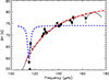 |
Fig. A.1. Variations in the g-mode period spacings as a function of mode frequency for KIC5180345. The observed period spacings (filled circles) were computed as the difference Δτ between the stretched periods τ of consecutive dipolar mixed modes (see Sect. 2.2). The blue dashed line indicates the g-mode period spacings for the best-fit buoyancy glitch perturbation. The red long-dashed line corresponds to the best-fit magnetic perturbation (see Sect. 4). For the magnetic perturbation, we also show the Δτ differences, which are directly comparable to the observations (black solid line). |
A.2. Glitch amplitude
We also addressed the question of the glitch amplitude that would be required to reproduce the observations. As shown in Fig. A.1, the observed deviations have an amplitude that reaches about 30% of the average period spacing. For comparison, Cunha et al. (2019) show the example of a Gaussian-shaped glitch in an RGB star, with an amplitude of about twice the local value of N and a width of about 0.001 R (see their Fig. 1). They find that it yields a modulation in the g-mode period spacing corresponding to only 1.5% of the asymptotic period spacing (see their Fig. 5).
To roughly estimate the glitch amplitude that would be needed in our case, we used the formalism of Cunha et al. (2019). We assumed a Gaussian-shaped buoyancy glitch and we used a Markov chain Monte Carlo (MCMC) to optimize the glitch properties (amplitude and width) in order to reproduce the observed g-mode period spacings as best as possible. Fig. A.1 shows the best-fit solution (blue dashed line). This fitting problem appears to be highly degenerated: similar profiles may be generated by different sets of parameters. However, some properties of the glitch can be derived from the MCMC. In particular, we conclude that its amplitude must be greater than six times the local value of N. All smaller values fail to reproduce the amplitude of the deviations observed in g-mode period spacings. However, even with the appropriate glitch amplitude, Fig. A.1 clearly shows that the best-fit solution cannot correctly reproduce the shape of the modulation. Indeed, it is well known (e.g., Miglio et al. 2008; Cunha et al. 2019) that large-amplitude glitches yield modulations in the g-mode period spacings that involve sharp localized features (as opposed to small glitches, which produce sinusoidal modulations), which seem incompatible with the smoothly varying period spacings that are observed. On the contrary, a magnetic perturbation to the oscillation modes provides a very good agreement with the observations (red and black lines in Fig. A.1).
Appendix B: Fit of asymptotic frequencies including magnetic perturbation
Fig. B.1 shows the stretched échelle diagrams of the detected dipole mixed modes for 11 red giants in our sample (blue circles). They were folded using the apparent (perturbed) period spacing  . In Sect. 4, we fit an asymptotic expression of the mode frequencies including a magnetic perturbation to the observed modes. The optimal solutions are shown in Fig. B.1 as red crosses. The agreement is very good. We give in Table B.1 the parameters of the best-fit solutions, along with general stellar properties, for each star.
Red giant branch stars showing strong variations in ΔΠ1 among the catalog of Yu et al. (2018).
Appendix C: Minimal field strength required to detect magnetic distortion in a g-mode pattern
We searched for the minimal field strength that produces a detectable deviation in the regular period spacing of pure gravity modes. For this purpose, we considered typical oscillation properties for red giants. More refined estimates could be obtained on a star-to-star basis, but for the purposes of this work we were interested in deriving broad estimates of magnetic intensity thresholds in order to investigate observational biases.
For a given red giant with a large separation Δν and a frequency of maximum power of the oscillations νmax, we consider that the modes can be detected in a frequency interval ranging from fmin = νmax − 2Δν and fmax = νmax + 2Δν. The asymptotic expression of unperturbed pure gravity modes is given by Pn = ΔΠ1(n + 1/2 + εg), so that we expect to detect g modes with radial orders ranging from nmin = 1/(ΔΠ1fmax)−εg − 1/2 and nmax = 1/(ΔΠ1fmin)−εg − 1/2. We then consider the asymptotic periods  of perturbed g modes in the presence of a field that produces a frequency shift δν0 at νmax. Assuming that the perturbation remains small compared to the mode periods themselves (this assumption holds at the detection limit for all stars of the sample), we have
 (C.1)
(C.1)
When analyzing the seismic data in red giants, high-radial-order gravity modes are assumed to be regularly spaced in a period and they are thus fit by an expression of the type  . Magnetic perturbations to the g-mode periods can be detected if the deviations compared to a regular spacing in a period, expressed as
  , are sufficiently large. Since the unperturbed periods Pn vary linearly with n, the deviations δPn can be written as
 (C.2)
(C.2)
where α and β are the parameters of a linear regression of the term  as a function of n. Eq. C.2 shows that the intensity of the deviation from a regular period spacing is proportional to δν0. This can also be seen in the measured period spacing
  , which corresponds to ΔΠ1 + αδν0 here.
The period differences can be translated into frequency differences as  . Fig. C.1 shows the variations in δνn as a function of n for an illustration case with Δν = 10.6 μHz, ΔΠ1 = 79.9 s, εg = 0.3, and δν0 = 0.4 μHz. The maximal values of |δνn| are reached at the boundaries of the interval, more particularly for n = nmin.
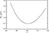 |
Fig. C.1. Departures from a regular period spacing of gravity modes in the presence of a magnetic field, shown as frequency differences δνn as a function of the radial order n of gravity modes. |
To determine whether these differences are detectable, we need to compare them with the frequency resolution of the measurements of oscillation mode frequencies. At the edge of the frequency interval where oscillations are detected, typical uncertainties reach several tens of nHz. We thus consider that a deviation from a regular period spacing can be detected if δνnmin exceeds a threshold δνth = 100 nHz. We subsequently obtained the following expression for the minimal detectable magnetic perturbation:
 (C.3)
(C.3)
We then used Eq. 5 to translate the minimal magnetic frequency shifts into minimal detectable field intensities Bth, which are shown in Fig. 3.
Appendix D: Dynamo-generated fields in main-sequence convective cores
The stars in which we detected strong core magnetic fields in this study have masses ranging from 1.11 to 1.56 M⊙ (see Table B.1). The lowest-mass stars of the sample have a radiative core during the largest part of their main-sequence evolution, but even these stars possess a small convective core at the beginning of the main sequence because of the burning of 3He and 12C outside of equilibrium. We tried to determine to what extent the detected fields are compatible with dynamo-generated fields in the main-sequence convective core.
For this purpose, we assumed that a uniform field Br, MS was produced during the main sequence, over a distance corresponding to the maximal extent of the convective core. After the withdrawal of the convective core, we assumed a conservation of the magnetic flux in each layer, so that the field intensity varies as 1/r(m)2 for a layer at Lagrangian coordinate m. We could then calculate the average field strength  at each step of the evolution. For each star of the sample, we calculated the intensity of the main-sequence radial field Br, MS that is required to produce the minimal average fields
  that we measured in Sect. 4. We thus found main-sequence field strengths ranging from about 1 to 26 kG (see Table D.1). These values correspond to lower limits on Br, MS, with the actual value depending on the geometry of the current radial magnetic field. For instance, if
  has an axisymmetric dipolar configuration (asymmetry parameter a = 2/5), the recovered values of Br, MS range from 1 to 40 kG.
Minimal main-sequence field intensities required to account for current measured fields in the cores of our sample of red giants, assuming conservation of the magnetic flux along the evolution.
All Tables
Red giant branch stars showing strong variations in ΔΠ1 among the catalog of Yu et al. (2018).
Minimal main-sequence field intensities required to account for current measured fields in the cores of our sample of red giants, assuming conservation of the magnetic flux along the evolution.
All Figures
|
Fig. 1. Stretched period échelle diagrams of two red giants showing distortion from the regular g-mode pattern. Blue circles show detected dipole modes. Red crosses correspond to the best-fit asymptotic mixed mode frequencies obtained by including a magnetic perturbation. |
| In the text | |
|
Fig. 2. Location of RGB stars with nonconstant ΔΠ1 in the (Δν, ΔΠ1) plane. Black star symbols correspond to the values of ΔΠ1 that produce the best vertical alignment of modes in the stretched period échelle diagram (Sect. 2). Colored star symbols correspond to the corrected values of ΔΠ1 obtained by taking into account the magnetic perturbation to the mode frequencies (Sect. 4). Other RGB stars from Vrard et al. (2016) are shown as gray circles (for clarity, stars flagged by the authors as potential aliases were omitted). |
| In the text | |
|
Fig. 3. Minimal field strength |
| In the text | |
|
Fig. 4. Power spectrum of KIC 6975038 obtained from Kepler data. Color-shaded areas indicate the location of l = 0 (blue), l = 1 (red), and l = 2 (green) modes. |
| In the text | |
|
Fig. A.1. Variations in the g-mode period spacings as a function of mode frequency for KIC5180345. The observed period spacings (filled circles) were computed as the difference Δτ between the stretched periods τ of consecutive dipolar mixed modes (see Sect. 2.2). The blue dashed line indicates the g-mode period spacings for the best-fit buoyancy glitch perturbation. The red long-dashed line corresponds to the best-fit magnetic perturbation (see Sect. 4). For the magnetic perturbation, we also show the Δτ differences, which are directly comparable to the observations (black solid line). |
| In the text | |
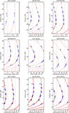 |
Fig. B.1. Same as Fig. 1, but for the remaining stars of the sample. |
| In the text | |
|
Fig. C.1. Departures from a regular period spacing of gravity modes in the presence of a magnetic field, shown as frequency differences δνn as a function of the radial order n of gravity modes. |
| In the text | |
Current usage metrics show cumulative count of Article Views (full-text article views including HTML views, PDF and ePub downloads, according to the available data) and Abstracts Views on Vision4Press platform.
Data correspond to usage on the plateform after 2015. The current usage metrics is available 48-96 hours after online publication and is updated daily on week days.
Initial download of the metrics may take a while.