| Issue |
A&A
Volume 689, September 2024
|
|
|---|---|---|
| Article Number | A337 | |
| Number of page(s) | 14 | |
| Section | Extragalactic astronomy | |
| DOI | https://doi.org/10.1051/0004-6361/202449147 | |
| Published online | 24 September 2024 | |
Investigating the nuclear properties of highly accreting active galactic nuclei with XMM-Newton
1
INFN – Sezione di Roma “Tor Vergata”, Via della Ricerca Scientifica 1, I-00133 Roma, Italy
2
Space Science Data Center, SSDC, ASI, Via del Politecnico snc, I-00133 Roma, Italy
3
INAF – Osservatorio Astronomico di Roma, Via Frascati 33, I-00078 Monte Porzio Catone, Italy
4
Dipartimento di Fisica, Università degli Studi di Roma “Tor Vergata”, Via della Ricerca Scientifica 1, I-00133 Roma, Italy
5
INAF – Istituto di Astrofisica e Planetologia Spaziali, Via del Fosso del Caveliere 100, 00133 Roma, Italy
6
ESA European Space Research and Technology Centre (ESTEC), Keplerlaan 1, 2201 AZ Noordwijk, The Netherlands
7
Dipartimento di Fisica e Astronomia ‘Augusto Righi’, Università degli Studi di Bologna, Via P. Gobetti, 93/2, 40129 Bologna, Italy
8
INAF – Osservatorio di Astrofisica e Scienza dello Spazio di Bologna, Via Piero Gobetti, 93/3, I-40129 Bologna, Italy
9
Dipartimento di Fisica “Ettore Pancini”, Università di Napoli Federico II, Via Cintia 80126, Italy
10
INAF – Osservatorio Astronomico di Capodimonte, Via Moiariello 16, 80131 Naples, Italy
11
INFN – Unità di Napoli, Via Cintia 9, 80126 Napoli, Italy
Received:
2
January
2024
Accepted:
10
July
2024
Highly accreting active galactic nuclei (AGNs) have unique features that make them ideal laboratories for studying black hole accretion physics under extreme conditions. However, our understanding of the nuclear properties of these sources is hampered by the lack of a complete systematic investigation of this AGN class in terms of their main spectral and variability properties, and by the relative paucity of them in the local Universe, especially those powered by supermassive black holes with MBH > 108 M⊙. To overcome this limitation, we present here the X-ray spectral analysis of a new, large sample of 61 highly accreting AGNs named as the XMM-Newton High-Eddington Serendipitous AGN Sample, or X-HESS, obtained by cross-correlating the 11th release of the XMM-Newton serendipitous catalogue and the catalogue of spectral properties of quasars from the SDSS DR14. The X-HESS AGNs are spread across wide intervals with a redshift of 0.06 < z < 3.3, a black hole mass of 6.8 < log(MBH/M⊙) < 9.8, a bolometric luminosity of 44.7 < log(Lbol/erg s−1) < 48.3, and an Eddington ratio of −0.2 < log λEdd < 0.5, and more than one third of these AGNs can rely on multiple observations at different epochs, allowing us to complement their X-ray spectroscopic study with a variability analysis. We find a large scatter in the Γ − λEdd distribution of the highly accreting X-HESS AGNs, in agreement with previous findings. A significant correlation is only found by considering a sample of lower-λEdd AGNs with λEdd ≲ 0.3. We get hints that the Γ − λEdd relation appears to be more statistically sound for AGNs with lower MBH and/or Lbol. We investigate the possibility of transforming the Γ − λEdd plane into a fully epoch-dependent frame by calculating the Eddington ratio from the simultaneous optical/UV data from the optical monitor, λEdd, O/UV. Interestingly, we recover a significant correlation with Γ and a spread roughly comparable to that obtained when Lbol is estimated from SDSS spectra. Finally, we also get a mild indication of a possible anti-correlation between Γ and the strength of the soft excess, providing hints that reflection from an ionised disc may be effective in at least a fraction of the X-HESS AGNs, though Comptonisation from hot and warm coronae cannot be ruled out as well.
Key words: galaxies: active / quasars: general / quasars: supermassive black holes
© The Authors 2024
 Open Access article, published by EDP Sciences, under the terms of the Creative Commons Attribution License (https://creativecommons.org/licenses/by/4.0), which permits unrestricted use, distribution, and reproduction in any medium, provided the original work is properly cited.
This article is published in open access under the Subscribe to Open model. Subscribe to A&A to support open access publication.
1. Introduction
Active galactic nuclei (AGNs) are powered by accretion processes onto a central supermassive black hole (SMBH). The accretion activity is usually parameterised by the Eddington ratio λEdd = Lbol/LEdd, where Lbol and LEdd represent the bolometric and Eddington1 luminosity, respectively. Highly accreting AGNs – that is, those with λEdd ≳ 0.6 – are characterised by some intriguing properties that make them interesting case studies.
First, the accretion flow in the low-to-moderate λEdd regime envisages an optically thick, geometrically thin disc that radiates efficiently (Shakura & Sunyaev 1973). The net effect of radiation pressure becomes prominent with increasing λEdd and, as a result, the disc thickens vertically. These systems are often called slim discs, as they are both optically and geometrically thick (e.g Abramowicz et al. 1988; Chen & Wang 2004; Sądowski et al. 2011). Slim discs are also expected to have a low radiative efficiency because of the photon-trapping effect. This mechanism contributes to saturating the observed disc luminosity (∼Lbol) to a limiting value of approximately 5−10 LEdd for steadily increasing accretion rates (e.g. Mineshige et al. 2000). Although the slim disc is expected to have peculiar properties in both its spectral energy distribution and its temperature profile compared to the standard disc model, it is often difficult to detect differences between high- and low-λEdd AGNs (e.g. Castelló-Mor et al. 2017; Liu et al. 2021; Cackett et al. 2020; Donnan et al. 2023).
The high-λEdd accretion mode is often considered in terms of its cosmological implications. Indeed, an increasing effort has been made in recent years to detect quasars (i.e. AGNs with Lbol > 1046 erg s−1; QSOs hereafter) at the distant redshift of z ∼ 6 − 7, corresponding to an age when the Universe was less than ∼1 Gyr old (e.g. Wu et al. 2015; Bañados et al. 2016; Mazzucchelli et al. 2017; Onoue et al. 2020; Ighina et al. 2021). These QSOs do typically host massive SMBHs – that is, ones with MBH ≥ 109 M⊙ – and the physical mechanism that allowed them to grow that massive in such a relatively short period of time is still debated. The evolution of these SMBHs via uninterrupted or rather intermittent episodes of gas accretion at a critical (or super-Eddington) rate is arguably one of the most commonly hypothesised mechanisms (e.g. Begelman et al. 2006; Inayoshi et al. 2016; Valiante et al. 2017; Zappacosta et al. 2020; Zhang et al. 2020; Lusso et al. 2023).
Furthermore, the launching of powerful disc winds, such as ultra-fast outflows (UFOs), is thought to occur naturally as a consequence of the high-λEdd accretion (e.g. Proga 2005; Zubovas & King 2013; King & Pounds 2015). These nuclear outflows are likely to have an impact on both the SMBH growth and the evolution of the host galaxy, by depositing large amounts of energy and momentum into the interstellar medium (e.g. Zubovas & King 2012), offering a possible explanation for the observed MBH − σ relation (e.g. Ferrarese & Merritt 2000). Consequently, the AGN feedback mechanism should manifest itself in full force in high-λEdd sources, making them the ideal laboratory for probing the impact of nuclear activity on the evolution of massive galaxies (e.g. Reeves et al. 2009; Nardini et al. 2015; Tombesi et al. 2015; Marziani et al. 2016; Bischetti et al. 2017, 2019; Laurenti et al. 2021; Luminari et al. 2021; Middei et al. 2023).
Despite all these remarkable features, high-λEdd AGNs have often been overlooked in the context of X-ray spectroscopic studies, probably due to their relative paucity in the local (z ≲ 0.1) Universe (e.g. Shankar et al. 2013; Shirakata et al. 2019). Indeed, the bulk of such works typically dealt with AGNs accreting at low-to-moderate Eddington rates (e.g. Nandra & Pounds 1994; Piconcelli et al. 2005; Bianchi et al. 2009; Liu et al. 2016; Ricci et al. 2018), with the notable exception of the Narrow Line Seyfert 1 galaxies (NLSy1s; Brandt et al. 1997; Gallo 2006; Costantini et al. 2007; Jin et al. 2013; Fabian et al. 2013; Waddell & Gallo 2020). However, among the high-λEdd systems, the NLSy1s represent a peculiar and restricted class of low-mass (106 − 107 M⊙) AGNs with the narrowest allowed emission lines in type-1 AGN samples (FWHM(Hβ) < 2000 km s−1; Osterbrock & Pogge 1985; Marziani et al. 2018). In this sense, they may be regarded as a biased population, and thus enlarging the parameter space of the relations involving λEdd and the main X-ray spectral parameters towards AGNs hosting more massive SMBHs is of crucial importance in the light of the currently hotly debated issues that we describe in the following.
First, several authors have reported on a positive correlation between the Eddington ratio and the photon index of the power-law continuum, Γ, from which we expect that AGNs accreting close to or above the Eddington limit will present steep values of Γ ≥ 2 (e.g. Shemmer et al. 2008; Risaliti et al. 2009; Brightman et al. 2013; Kawamuro et al. 2016; Huang et al. 2020). The general interpretation is based on the assumption that the enhancement of the optical/UV emission due to high-λEdd accretion increases the number of seed photons undergoing Comptonisation in the X-ray corona. As the cooling process in the corona becomes more efficient, its temperature decreases and the primary X-ray continuum becomes progressively softer. This relation elicited immediate interest, especially for its possible applications in X-ray extragalactic surveys, since it would allow us to obtain an estimate of MBH from the X-ray spectrum, including that of type-2 AGNs for which commonly used ‘single-epoch’ estimators are not applicable. However, recent works questioned the existence of a strong correlation between Γ and λEdd, with some authors reporting only a weaker (e.g. Ai et al. 2011; Kamizasa et al. 2012; Martocchia et al. 2017; Trakhtenbrot et al. 2017; Kamraj et al. 2022; Trefoloni et al. 2023) or even no correlation (e.g. Liu et al. 2016) between these two parameters, which highlights the need to study this relation in more detail.
In addition, Lusso et al. (2010) claimed the existence of a positive correlation between λEdd and both the X-ray bolometric correction, kbol, X = Lbol/L2 − 10 keV, and the optical/UV-to-X-ray spectral index, αox, for a large sample of type-1 (i.e. unobscured) AGNs in the COSMOS survey, extending over wide intervals of redshift (0.04 < z < 4.25) and bolometric luminosity (40.6 < log(Lbol/erg s−1) < 45.3). A more refined version of the kbol, X − λEdd relation has recently been provided by Duras et al. (2020), who found that  for an AGN sample in which a sizeable number of highly accreting sources at z ∼ 2 − 4 was also included. According to these relations, one would expect that the coupling between the X-ray corona and the accretion disc is such that, for increasingly large values of λEdd, it attains a configuration leading to a dimming of the X-ray primary continuum with respect to the optical/UV emission from the disc, compared to ‘standard’ AGNs.
However, both results and expectations based on the above relations are hampered by the limited number of high-λEdd AGNs, especially ones hosting more massive SMBHs, which were actually available in most of those studies. To overcome this limitation, in Laurenti et al. (2022) we performed an X-ray spectroscopic analysis of a sample of fourteen XMM-Newton (Jansen et al. 2001) observations of type-1 radio-quiet QSOs accreting in a narrow interval of λEdd values with λEdd ≳ 0.9 at a redshift of z ∼ 0.4 − 0.75. These AGNs were drawn from a larger sample of highly accreting sources sharing homogenous optical/UV properties described in Marziani & Sulentic (2014), and are characterised by large black hole mass values of MBH ∼ 108 − 8.5 M⊙ derived from the full width at half maximum (FWHM) of the Hβ emission line. Despite all these QSOs possessing similar λEdd values, we found that Γ was characterised by a large dispersion, with values ranging from a minimum of ∼1.3 to a maximum of ∼2.5, at odds with the expectations based on several of the previously reported Γ − λEdd relations. Moreover, the results of our best-fit spectral analysis indicated that approximately ∼30% of the QSOs in our sample displayed weak X-ray emission, which could not be ascribed to cold absorption.
Since our previous findings suggest that our understanding of the high-λEdd accretion mode in AGNs is still incomplete, it is evident that this study would benefit from a larger number of observations of highly accreting sources. Fortunately, many of these highly accreting objects can be serendipitously found in the field of view of other X-ray sources that have been intensively and repeatedly targeted thanks to deep observational campaigns, such as those carried out with XMM-Newton. The analysis of serendipitous high-λEdd AGNs discloses the unprecedented possibility of investigating not only their spectral but also variability properties in the X-rays in a much wider range of black hole mass, bolometric luminosity, and redshift.
For this reason, we present the spectroscopic and variability study of a large sample of high-λEdd AGNs named as the XMM-Newton High-Eddington Serendipitous AGN Sample, or X-HESS, with the aim of continuing our quest to uncover the properties of such highly accreting systems. The paper is organised as follows. We describe the procedure that leads to the definition of the sample and its general properties in Sect. 2. Section 3 is dedicated to the description of the X-ray spectroscopy as well as the optical/UV photometry of our sample sources. We then present our results in Sects. 4 and 5. Finally, we draw our conclusions in Sect. 6. Appendices A–C have been uploaded to Zenodo2. A ΛCDM cosmology with H0 = 70 km s−1 Mpc−1, Ωm = 0.3 and ΩΛ = 0.7 is adopted throughout the paper. All errors are quoted at the 68% confidence level (ΔW-stat = 1; Avni 1976; Cash 1979; Wachter et al. 1979). In the following, correlations will be considered statistically significant based on the significance level of α = 10−3.
2. Sample description
In order to define a large sample of high-λEdd serendipitous AGNs, we chose to exploit the extended database included in the 11th release of the XMM-Newton Serendipitous Source Catalogue (4XMM-DR11; Webb et al. 2020), which contains 12 210 observations carried out between February 2000 and December 2020, in which approximately ∼900 000 sources have been detected. To retrieve only those X-ray observations of spectroscopically confirmed AGNs, we considered the catalogue of spectral properties of QSOs from the Sloan Digital Sky Survey Data Release 14 Quasar Catalogue (SDSS-DR14Q; Pâris et al. 2018) described in Rakshit et al. (2020), which includes measurements of the main physical quantities of ∼526 000 AGNs, and cross-matched it with the serendipitous XMM-Newton catalogue within a radius of 3 arcsec in coordinates to avoid possible spurious identifications, while maximising the completeness of the sample. Then we imposed the additional requirements that (i) each source with multi-epoch detections must have at least one good quality observation in terms of photon counts in the broad (E = 0.2 − 12 keV) EP8 band–that is, EP_8_CTS ≥ 1000 – to ensure robust spectral results, and (ii) only those AGNs with a sufficiently high value of log λEdd that we set to log λEdd ≥ −0.2 would be considered. At this stage, we obtained a sample of 95 AGNs for a total of 217 observations. Since we are only interested in standard radio-quiet AGNs, we removed twenty sources that have been either classified as radio-loud or known to be lensed from the sample. Starting from this sample of 75 AGNs, we imposed the further condition that the MBH estimate of each source must be derived from the FWHM of either Hβ or Mg II emission lines, which are more reliable estimators than the FWHM of C IV (e.g. Baskin & Laor 2005; Coatman et al. 2017; Vietri et al. 2018, 2020). Two AGNs–namely, J0900+4215 and J1326−0005 – for which the sole C IV black hole mass is provided in the catalogue of Rakshit et al. (2020) are also included in the final sample, because they are part of the WISE/SDSS selected hyper-luminous quasar sample (WISSH; Bischetti et al. 2017) and can benefit from refined Hβ-based MBH estimates as well as more refined measurements of Lbol (Vietri et al. 2018). For the rest of the X-HESS AGNs, we adopted the Lbol values from Rakshit et al. (2020) that were derived from the bolometric corrections in Richards et al. (2006) involving the monochromatic luminosities at 5100 Å (z < 0.8), 3000 Å (0.8 ≤ z < 1.9), or 1350 Å (z ≥ 1.9). Finally, we obtained a catalogue of 61 AGNs with 142 observations that we named the XMM-Newton High-Eddington Serendipitous AGN Sample, or X-HESS.
The X-HESS AGNs are distributed over wide intervals of bolometric luminosity (44.7 < log(Lbol/erg s−1) < 48.3), black hole mass (6.8 < log(MBH/M⊙) < 9.8), redshift (0.06 < z < 3.3), and Eddington ratio (−0.2 < log λEdd < 0.5). The presence of AGNs spanning a wide range of MBH, Lbol, and z contributes to making X-HESS a useful tool with which to improve our understanding of high-λEdd AGNs in regions of the parameter space that have been poorly sampled so far. Specifically, the broad MBH and Lbol distributions of the X-HESS AGNs (see Fig. 1) allow us to extend the analysis of highly accreting sources towards AGNs with both bolometric luminosity and a black hole mass substantially higher than those previously considered in other studies (e.g. Lu et al. 2019; Liu et al. 2021).
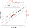 |
Fig. 1. Distribution of the X-HESS AGNs in the log Lbol − log MBH plane (in black). Red squares indicate the high-λEdd local AGN subsample from Liu et al. (2021), as a comparison. With respect to this sample, the X-HESS AGNs extend towards larger values of both bolometric luminosity and black hole mass. Dash-dotted black lines describe different values of λEdd. |
Figure 2 shows the z − λEdd distribution of the X-HESS sources, where AGNs with individual or multi-epoch observations are shown in the same plot. The multi-epoch subsample of X-HESS is well representative of the whole sample in terms of these quantities and the same holds for other physical parameters such as MBH and Lbol, offering the unprecedented opportunity to investigate the X-ray flux and spectral variability of 22 highly accreting sources that have been repeatedly observed by XMM-Newton for a total of 103 times.
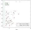 |
Fig. 2. Distribution of the X-HESS AGNs in the z − λEdd plane. All the X-HESS AGNs and the subsample with multi-epoch observations are described by grey dots and red diamonds, respectively. The multi-epoch subsample is well representative of the whole sample in terms of these quantities. |
Furthermore, we can complement X-HESS with simultaneous optical/UV data, allowing us to investigate the interplay with the X-rays (e.g. with αox), by taking advantage of the observations carried out by the Optical Monitor (OM; Mason et al. 2001) aboard XMM-Newton. Indeed, a sizeable fraction of the X-HESS sources (∼62%) can rely on simultaneous OM observations obtained by crossmatching X-HESS with the latest release of the XMM-OM Serendipitous Ultraviolet Source Survey Catalogue (SUSS5.0; Page et al. 2012). An overview of the X-HESS AGNs, including their general properties, is provided in Appendix A.
3. Data analysis
3.1. Data reduction
The raw data for each observation of the X-HESS AGNs were retrieved from the XMM-Newton Science Archive and then processed using the XMM-Newton Science Analysis System (SAS v21.0.0) with the latest available calibration files. We took advantage of the full potential of XMM-Newton in the X-ray energy interval E = 0.3 − 10 keV (observer frame) by collecting data from its primary instrument, the European Photon Imaging Camera (EPIC), which is equipped with three X-ray charge-coupled device cameras; namely, the pn (Strüder et al. 2001) and the two MOS detectors (Turner et al. 2001). Data reduction, filtering of high background periods, and spectral extraction were performed according to the standard procedures described on the SAS web page3. For each object, we chose a circular region with a radius of ∼20 − 30 arcsec for the source extraction, corresponding to ≥70% of the encircled energy fraction for both on-axis and off-axis sources and a nearby, larger source-free circular region for the background. The spectra were binned to ensure at least one count per bin and modelled within the XSPEC (v12.13.0g; Arnaud 1996) package by minimising the Cash statistic with background subtraction (W-stat in XSPEC; Cash 1979; Wachter et al. 1979).
3.2. X-ray spectroscopy
We adopted the following procedure to analyse the X-ray spectrum of each source in our sample. Data from EPIC-pn, MOS1, and MOS2 were always considered simultaneously and fitted together, taking into account an intercalibration constant between the three instruments that was allowed to vary within a factor of < 20%. This threshold is less strict than that typically adopted in the case of dedicated on-axis pointings (Read et al. 2014), as in this work we deal with observations of serendipitous AGNs that are likely to be positioned off-axis with respect to the centre of the XMM-Newton field of view (see, e.g. Mateos et al. 2009). While the off-axis position leads to an increased vignetting and elongated point spread function that may have an impact on the cross-calibration of EPIC cameras (e.g. Mateos et al. 2009; Read et al. 2011), it also implies, as an aside, that sometimes the given source can lie within a bad column or a gap between the CCDs. For this reason, for each X-HESS AGN, we checked whether any of these occurrences were actually present in the observations carried out with the EPIC cameras and then we considered only those data unaffected by such limitations to extract the X-ray spectrum.
Figure 3 provides a general description of all the 142 XMM-Newton observations of the X-HESS AGNs in terms of the photon counts in the broad E = 0.3 − 10 keV observer-frame energy interval, showing the relative frequency histogram of the cumulative net (i.e., background-subtracted) counts calculated by considering the joint EPIC-pn, MOS1, and MOS2 observations. This distribution is characterised by a median value of ∼900 and is indicative of the spectral quality of the X-HESS observations, with more than 90% (40%) of their total having a number of counts of > 100 (> 1000). The comprehensive journal of observations of the X-HESS AGNs can be consulted in Appendix B, where the reader can find information about both the net exposure and counts for all the EPIC cameras in Table B.1.
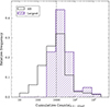 |
Fig. 3. Relative frequency histogram showing the distribution of the total net counts from EPIC-pn, MOS1, and MOS2 in the broad E = 0.3 − 10 keV observer-frame energy band for each individual observation of the X-HESS AGNs (in black). The distribution related to the observations with the largest number of counts of each X-HESS AGN is shown in purple. |
For each spectrum, we first ignored all the data outside the E = 0.3 − 10 keV observer-frame energy interval and then initially considered the hard X-ray spectrum (E > 2 keV in the rest frame, corresponding to E > 2/(1 + z) keV in the observer frame), to constrain the value of the photon index without any possible contamination from additional spectral components such as the soft excess – likely to emerge at softer energies – that could affect the Γ measurement. The determination of the underlying primary continuum was achieved by modelling the hard X-ray spectrum with a power law modified by Galactic absorption. Then we extended the analysis to the broad E = 0.3 − 10 keV interval by including the soft portion of the X-ray spectrum. Eventually, further deviations in the residuals were addressed by considering additional spectral components, which were included in the best-fit model whenever appropriate; that is, according to the statistical significance of the ΔW-stat value with respect to the corresponding change of degrees of freedom at a 95% confidence level for the number of interesting parameters characterising the additional component.
Though the observations with a larger number of counts are likely to return a more detailed view of the AGN spectral features, our best-fit spectral results suggest that the broadband X-ray continuum (E = 0.3 − 10 keV) of the X-HESS sources can always be reproduced by a phenomenological model consisting of a power law modified by Galactic absorption plus, in some cases, a blackbody component to account for the excess of soft X-ray emission that characterises more than a third of all the 142 observations. Indeed, as is shown in Fig. 4, the former model accounts for the X-ray continuum emission of ∼60% of the observations of the X-HESS AGNs, while the latter indicates that ∼40% of the spectra reveals the presence of a soft excess.
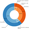 |
Fig. 4. Pie chart describing the overall results of the spectroscopic analysis of the X-HESS sources. In most cases, the broadband X-ray continuum (E = 0.3 − 10 keV) can be reproduced well by a power-law model, modified by Galactic absorption. In the remaining ∼40% of the observations, an excess of soft X-ray emission is found. Approximately ∼12% of the X-ray spectra of the X-HESS AGNs reveal the presence of at least one emission and/or absorption feature due to the interaction of the primary continuum with either cold or ionised gas clouds. |
Although the blackbody model provides only a phenomenological explanation of the soft excess, whose physical origin is still debated (e.g. Sobolewska & Done 2007; Fukumura et al. 2016; Petrucci et al. 2018; Middei et al. 2020), it also offers the best description of the soft excess in terms of the W-statistic for all the spectra showing such a feature. Moreover, we find values of blackbody temperature, kTbb, that are consistent with those typically measured for type-1 AGNs (e.g. Piconcelli et al. 2005; Bianchi et al. 2009), ranging from a minimum of ∼100 eV up to ∼350 eV.
While such basic modelling returns a satisfactory description of the vast majority of the broadband X-ray spectra (∼88%), as is shown in Fig. 4, we find evidence of at least one emission and/or absorption feature in approximately ∼12% of the observations due to the interaction of the primary continuum with either cold or ionised gas clouds. In the latter case, the absorption features are usually attributable to either warm absorbers (WAs) or UFOs. However, we note that this fraction is most likely a lower limit because of the limited S/N of several observations. We refer the reader to Appendix C for a thorough description of the best-fit spectral results, where one can also find a few additional notes about those AGNs with relatively more complex spectra.
3.3. Measuring the ultraviolet luminosity and αox
3.3.1. Optical Monitor data reduction
When available, the XMM-Newton observations were complemented with the simultaneous optical/UV data from the Optical Monitor. The raw OM data were converted to science products using the SAS task omichain. We used the task om2pha to convert the OM photometric points into a suitable format for XSPEC. Galactic extinction was taken into account by considering the measurement of the colour excess from the reddening map of Schlafly & Finkbeiner (2011), provided by the NASA/IPAC Infrared Science Archive (IRSA) website4. The spectra were then corrected for Galactic extinction according to the Milky Way reddening law of Fitzpatrick (1999), assuming RV = 3.1.
3.3.2. L2500 Å and αox
The OM measurements allowed us to estimate the monochromatic UV luminosity of L2500 Å by adopting the approach described in Vagnetti et al. (2010), which can be summarised as follows: (i) When the available rest-frame luminosity estimates from the OM filters only cover frequencies higher or lower than 2500 Å, L2500 Å was calculated through curvilinear extrapolation, following the behaviour of the average optical/UV spectral energy distribution of Richards et al. (2006), computed for a large sample of type-1 AGNs with SDSS data coverage, shifted vertically to match the specific luminosity at the frequency of the nearest OM data point. (ii) If the OM data points extend across rest-frame λ = 2500 Å, L2500 Å was calculated with a linear interpolation. (iii) When only a single OM filter was available, L2500 Å is measured as in (i). We estimate the luminosity at λ = 4400 Å, whose usage will be discussed in the Sect. 4.4, in a similar fashion. The values of both L2500 Å and L4400 Å are listed in Table C.1.
We estimated the possible contribution of the host galaxy starlight to the optical/UV emission by modelling the optical spectrum as a combination of AGN and galaxy components, following the procedure described in Vagnetti et al. (2013). We find that the host galaxy contribution is less than 10% for the bulk of the sample and can be safely neglected for all the X-HESS sources.
Moreover, we measured the internal reddening of the X-HESS AGNs by adopting an approach similar to that described in Laurenti et al. (2022). For each source, we compared the SDSS spectrum with the SDSS composite QSO’s spectrum by Vanden Berk et al. (2001) and normalised them to the unit flux at rest-frame wavelengths corresponding to λobs ≥ 8000 Å in the observer frame. We then applied the Small Magellanic Cloud (SMC) extinction law by Prevot et al. (1984) to the template, as is shown in Fig. 5. The choice of an SMC-like extinction law stems from its capability of reproducing dust reddening of QSOs at all redshifts (e.g. Richards et al. 2003; Hopkins et al. 2004; Bongiorno et al. 2007; Gallerani et al. 2010; Krawczyk et al. 2015). In each case, the fiducial value of E(B − V) is the one that minimises the distance between the template and the SDSS spectrum at wavelengths shorter than λobs = 8000 Å. The vast majority of the sources – ∼85% – do have E(B − V)≤0.1, while the rest of the AGNs present reddening values extending up to a maximum of ∼0.33. The typical uncertainty on these reddening estimates is ∼0.01. The values of internal reddening of the X-HESS AGNs are reported in Table A.1. The OM photometric data were then corrected for the effects of both Galactic and internal dust extinction to obtain a refined measurement of L2500 Å. In principle, the OM data variability for the multi-epoch AGNs may be due to a combination of possible changes in the accretion rate and/or extinction, which are not easy to disentangle. Moreover, multi-epoch optical spectra would be required as well to provide deeper insights into the possible extinction changes.
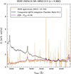 |
Fig. 5. SDSS spectrum of J0234−08 (X-HESS 7) at z = 0.992 (in gold) compared to the composite QSO’s template of Vanden Berk et al. (2001). The template (in black) is extinguished according to the SMC extinction law by Prevot et al. (1984), with progressively increasing values of E(B − V). The value of E(B − V) that minimises the distance between the reddened template (in purple) and the observed SDSS spectrum at wavelengths of λobs < 8000 Å in the observer frame, corresponds to our estimate of the internal reddening of the source. J0234−08 has the largest E(B − V) among our sources, i.e. E(B − V) = 0.33. |
Finally, the value of the monochromatic UV luminosity, L2500 Å, can be used jointly with the monochromatic X-ray luminosity at 2 keV measured from the X-ray spectrum to calculate the αox parameter as
![$$ \begin{aligned} \begin{aligned} \alpha _{\rm ox}&= \log {\Bigg [\frac{L_\nu (2\,\mathrm{keV})}{L_\nu (2500\,\AA )}\Bigg ]}\,\Bigg /\,\log {\Bigg [\frac{\nu (2\,\mathrm{keV})}{\nu (2500\,\AA )}\Bigg ]} \\&\simeq 0.384\,\log {\Bigg [\frac{L_\nu (2\,\mathrm{keV})}{L_\nu (2500\,\AA )}\Bigg ]}\cdot \end{aligned} \end{aligned} $$](/articles/aa/full_html/2024/09/aa49147-24/aa49147-24-eq2.gif)
Clearly, the αox parameter could only be obtained for those 38 X-HESS AGNs with OM data coverage, 14 of which have multi-epoch observations. In total, there are 82 OM observations of the X-HESS AGNs and the corresponding αox values are listed in Table C.1.
3.3.3. X-ray weakness
Laurenti et al. (2022) found a significant population of X-ray weak sources among optically selected QSOs with Lbol > 1046 erg s−1, comprising almost 30% of their whole sample, and similar results were reported by Nardini et al. (2019) and Zappacosta et al. (2020), but this is not the case for the X-HESS sources. Figure 6 shows the distribution of the X-HESS AGNs with available OM measurements in the αox − log LUV plane, where log LUV is the luminosity at 2500 Å, also indicating the threshold for X-ray weakness defined by Pu et al. (2020). We recall that this threshold amounts to Δαox ≤ −0.3, with Δαox representing the difference between the observed value of αox and the expected value from the reference relation which, in our case, is that from Lusso et al. (2010). One can notice that in the vast majority of observations, the sources are distributed accordingly to the αox − log LUV relation from Lusso et al. (2010), while only a few observations of X-HESS AGNs included in the multi-epoch subsample are consistent with an epoch of weak X-ray emission. This result is not surprising, as it is probably due to the selection criteria of the X-HESS sources. Indeed, in building the sample we only considered those AGNs that have at least one observation with a sufficiently large number of photon counts in the EP8 band; that is, EP_8_CTS ≥ 1000. In this way, we are neglecting most of the highly accreting AGNs that are also X-ray weak, as for these sources we expect photon counts to be smaller than the one we adopted as a threshold. In order to investigate the true fraction of X-ray weak sources among the high-λEdd population, it would be necessary to significantly reduce such a limiting value for the photon counts – or better, and ideally remove it – though this would require a spectroscopic analysis of a huge number of AGNs, which was not feasible in this work. Despite this limitation, an interesting result is clearly emerging in Fig. 6 for SDSS J130048.10+282320.6 and SDSS J022928.41−051125.0; that is, X-HESS 5 and 16, respectively. Specifically, the time evolution of αox for X-HESS 5 and 16, described by the green and blue lines in the same figure, suggests that these sources have experienced at least one transition between phases of standard and weak X-ray emission over the different observations. This result is consistent with our findings based on the ongoing Swift monitoring of the X-ray weak AGNs described in Laurenti et al. (2022), which we shall present in a forthcoming paper (Laurenti et al., in prep.), in which we observe similar transitions between hard- and low-flux states in some sources, and thus supports the idea that the X-ray weakness of high-λEdd AGNs may represent a transient phenomenon over different timescales.
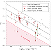 |
Fig. 6. Distribution of the X-HESS AGNs in the αox − log LUV plane. Single- and multi-epoch AGNs are shown in grey and red, respectively. White circles with red edges highlight the high-flux state of the multi-epoch X-HESS AGNs. Solid and dashed black lines indicate the best-fit relation from Lusso et al. (2010) and the corresponding 1σ spread. The solid red line marks the reference value for X-ray weakness, i.e. Δαox ≤ −0.3 (Pu et al. 2020). Dotted and dash-dotted blue and green lines describe the time evolution of αox for the AGNs X-HESS 16 and X-HESS 5, respectively. Specifically, the latter has experienced a couple of transitions between phases of standard and weak X-ray emission over the different observations. |
In the case of X-HESS 16 (z = 0.307), the transition towards the X-ray weak state occurs at ∼18 months in the source rest-frame. The soft and hard X-ray fluxes drop by a factor of approximately ∼5 and ∼3, respectively, and the photon index becomes shallower, moving from ∼1.8 to ∼1.3. For X-HESS 5 (z = 1.929), instead, we observe two transitions from and to an X-ray weak state. In both cases, the soft and hard X-ray fluxes drop or raise by a factor of ∼3 and ∼2, respectively, and the associated timescales are much shorter than for X-HESS 16, since each transition occurs over a period of ≲1 week in the source rest-frame. The value of the photon index, Γ, is consistent within the errors between the X-ray weak state (Γ ∼ 1.4) and the two contiguous higher-flux states (Γ ∼ 1.7), although it is slightly flatter in the former. It is also worth mentioning that the results of our spectroscopic analysis suggest that the X-ray weak state is not directly ascribable to cold absorption. This holds not only for X-HESS 5 and 16, but also for the single-epoch X-HESS 43 caught in a low-flux state (grey dot in Fig. 6). However, we cannot rule out the presence of a highly ionised gas cloud with a large column density and a small covering factor along the line of sight, which would cause a decrease in the X-ray flux without heavily affecting the spectral shape (see, e.g. Laurenti et al. 2022 for a detailed discussion). The remaining AGN lying in the X-ray weak domain is X-HESS 20, whose spectrum shows an absorption feature attributable to a warm gas cloud (see also Appendix C). Unlike the variable X-ray emission, the UV luminosity at 2500 Å remains relatively stable between normal and weak X-ray emission phases for both X-HESS 5 and 16.
We note that the hypothetical presence of broad-absorption line (BAL) QSOs can potentially affect the fraction of X-ray obscured sources among high-λEdd AGNs. Unfortunately, we cannot quantify their impact in the present study, as we were unable to retrieve this information on the presence of BAL features (e.g. C IV absorption) in the X-HESS sample.
4. Results
4.1. Spectral variability
The multi-epoch X-HESS AGNs allow us to investigate the spectral variability properties of these highly accreting sources. To track these variations, it is useful to consider the change in Γ values between the observations associated with the lowest- and highest-flux states of each individual AGN, respectively. Specifically, we can compute the fractional variations of both the photon index and E = 2 − 10 keV luminosity, LX, between the two observations of interest, Δγ = (Γhigh − Γlow)/Γlow and ΔℓX = (LX, high − LX, low)/LX, low, with a clear reference to the low- and high-flux states.
Figure 7 shows the Δγ − ΔℓX plane. The overall trend appears to favour positive variations in the photon index with increasingly larger changes in the hard X-ray luminosity, in agreement with a softer-when-brighter behaviour that is often reported in AGNs with a moderate-to-high Eddington ratio (e.g. Paolillo et al. 2004; Shemmer et al. 2006; Sobolewska & Papadakis 2009; Gibson & Brandt 2012; Soldi et al. 2014; Vagnetti et al. 2016; Serafinelli et al. 2017), though it is not highly significant since the Spearman’s correlation coefficient and the corresponding null probability are ρS = 0.40 and p(> |ρs|) = 0.07, respectively. Moreover, a minor fraction of the multi-epoch X-HESS AGNs appear to vary accordingly to the opposite trend; that is, harder when brighter.
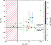 |
Fig. 7. Spectral variation in the photon index, Γ, versus the change in E = 2 − 10 keV X-ray luminosity between the lowest- and highest-flux states of the multi-epoch X-HESS AGNs. Luminosity changes of < 1% occurring within the red-hatched region are considered insignificant. Most of the sources vary accordingly to a softer-when-brighter trend, while a smaller fraction do the opposite. No clear correlation is found between the amplitude of the spectral variations and the time elapsed between the two observations of interest. |
Those AGNs with ΔℓX < 1% in terms of their nominal value or within their 1σ measurement error are considered as non-variable (red-shaded region in the plot). The same occurs for those sources whose Δγ is consistent with zero. Thus, we find that 14 of the 22 multi-epoch X-HESS AGNs (∼64%) do not show significant spectral variations between their corresponding lowest- and highest-flux observations. The eight remaining AGNs (∼36%) are characterised by significant spectral variations at the 1σ confidence level, with seven of them showing a softer-when-brighter trend, while only one source (X-HESS 11) does the opposite. The same figure shows the time elapsed between the two observations of interest for each source, and the amplitude of the spectral variations does not show a clear dependence in terms of such a time span, although half of the significant Γ changes apparently occur within a two-year rest-frame. Furthermore, it is worth noting that the multi-epoch X-HESS sources have not been monitored with a uniform cadence or an equal number of times, and this could possibly affect the distribution in the Δγ − ΔℓX plane.
4.2. The Γ − λEdd relation
We investigated the Γ − λEdd relation as follows. We constrained the X-ray primary continuum and derived the best-fit value of the photon index, Γ, of the X-HESS AGNs according to the procedure described in Sect. 3.2 for the X-ray spectral analysis, while the value of the Eddington ratio for each of these sources is listed in Table A.1. In this section and in Sect. 4.3, for the multi-epoch X-HESS AGNs, we only considered the value of the photon index in their highest-flux state, assuming that it most likely represents their intrinsic X-ray coronal emission if their lower-flux states were due to any kind of possible obscuration that in some cases might be potentially undetectable, as in lower S/N observations. The following results, however, still hold when jointly accounting for or averaging all the flux states of the multi-epoch X-HESS AGNs.
Figure 8 shows the distribution of the X-HESS AGNs in the Γ − log λEdd plane. When accounting for both the multi- and single-epoch X-HESS subsamples, we observe a large dispersion of Γ values spanning from a minimum of ∼1.5 to a maximum of ∼2.5, which is consistent with the range reported in Laurenti et al. (2022). However, in that case, we studied an AGN sample comprising sources lying in a narrow interval of λEdd values tightly clustered around log λEdd ∼ 0, while in this case we observe the same scatter when investigating the spectral properties of AGNs with −0.2 < log λEdd < 0.5. This may suggest that such a dispersion is a property of high-λEdd AGNs as a class and is likely to emerge whenever a sufficiently large sample of highly accreting sources is considered. We do not find any indication of a significant correlation between Γ and log λEdd, with the Spearman’s correlation coefficient being ρS = 0.21 for a null probability of p(> |ρS|) = 0.11. If we only consider the multi-epoch X-HESS AGNs, the correlation becomes weakly significant, as we find ρS = 0.54 and p(> |ρS|) ∼ 0.01, but it is still dominated by a large scatter.
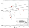 |
Fig. 8. Distribution of the X-HESS AGNs in the Γ − log λEdd plane. Single- and multi-epoch AGN are represented by grey circles and red diamonds, respectively. The best-fit relations from previous studies are reported as well. The average uncertainty on λEdd is 0.3 dex. |
To assess the relationship between Γ and λEdd, one needs to extend its dynamical range by including AGNs characterised by lower Eddington ratios. In their recent work, Liu et al. (2021) did study a sample of 47 local AGNs divided into two groups consisting of 21 high-λEdd and 26 low-λEdd AGNs, respectively, in which the dividing line was set at λEdd ∼ 0.3. All of these AGNs are located at a redshift of z ≲ 0.3 and can rely on very good quality MBH measurements from reverberation mapping. Moreover, the authors only considered the highest-flux observation of their AGNs, when available, to investigate the relation between the photon index at the E > 2 keV rest frame and λEdd. In our case, the Γ values reported in Table C.1 refer to the broadband E = 0.3 − 10 keV spectral fit but, as is discussed in Sect. 3.2, they were first constrained in the rest-frame E > 2 keV interval. For this reason, we can safely compare our results with those in Liu et al. (2021).
Figure 9 displays the distribution of the X-HESS AGNs and the two subsamples of local AGNs from Liu et al. (2021) in the Γ − log λEdd plane. Interestingly, if we consider both the X-HESS and high-λEdd local AGNs, the correlation between the two quantities is still not statistically sound, as ρS = 0.25 and p(> |ρS|) = 0.03. However, when considered altogether, the three samples show a highly significant correlation between Γ and λEdd, with the Spearman’s coefficient being ρS = 0.52 for a null probability of p(> |ρS|) < 10−7. Though this result is obviously driven by the low-λEdd AGN population in Liu et al. (2021), we computed the best-fit relation by adopting a bootstrap method; that is, by resampling N = 10 000 times the distribution in the Γ − log λEdd plane, while accounting for the errors in both variables. According to this procedure, we obtain
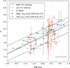 |
Fig. 9. Distribution of the X-HESS AGNs (orange circles) and the high-λEdd (blue squares) and low-λEdd local AGNs (red triangles) from Liu et al. (2021) in the Γ − log λEdd plane. For the multi-epoch X-HESS AGNs, we considered the Γ associated with their high-flux state. The black error bar in the lower right corner represents the average uncertainty on the X-HESS sources. Solid and dashed black lines describe the best-fit relation and its 1σ spread, respectively. The dash-dotted green line represents the Liu et al. (2021) best-fit relation, for comparison. |

The 1σ spread of the above relation is ∼0.22 and its slope is flatter – albeit consistent within the uncertainties – than the value of 0.27 ± 0.04 in Liu et al. (2021) and also shallower than that reported in the bulk of previous works (e.g. 0.31 ± 0.01, Shemmer et al. 2008; 0.31 ± 0.06, Risaliti et al. 2009; 0.56 ± 0.08, Jin et al. 2012; 0.32 ± 0.05, Brightman et al. 2013), while it can better adhere to more conservative findings (e.g. 0.17 ± 0.04, Trakhtenbrot et al. 2017; 0.16 ± 0.03, Trefoloni et al. 2023) envisaging a weaker Γ − log λEdd relation.
4.3. The role of MBH and Lbol in Γ − logλEdd
The Γ − log λEdd plane in Fig. 9 is populated by a variety of sources spanning from local Seyfert-like galaxies to moderate-to-high-redshift QSOs, and thus is characterised by very different physical and observational properties. Since the Eddington ratio is proportional to both MBH and Lbol, we tried to determine whether these quantities have an impact on the observed distribution.
We considered the X-HESS and both Liu et al. (2021) local AGN samples as a whole and then divided all sources into two equally populated subsamples in terms of MBH and Lbol. Specifically, we chose log(MBH/M⊙) = 8 and log(Lbol/erg s−1) = 45.5 as the thresholds on the black hole mass and the bolometric luminosity, respectively. These thresholds are almost consistent with the transition between the average properties of NLSy1s and QSOs.
The distribution of all sources in the Γ − log λEdd plane, highlighting the two different MBH (top panel) and Lbol (bottom panel) subsamples, is shown in Fig. 10. We find that the lower-MBH AGNs are highly correlated with the Eddington ratio (ρS = 0.62, p(> |ρS|) < 10−7) as opposed to the higher-MBH sample that has ρS = 0.28 and p(> |ρS|) = 0.06. We obtain a similar result for the Lbol subsamples, with the lower-Lbol AGNs being correlated with λEdd (ρS = 0.52, p(> |ρS|) = 10−4), while the higher-Lbol AGNs have ρS = 0.24 and p(> |ρS|) = 0.07.
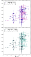 |
Fig. 10. Distribution of the X-HESS AGNs and the high-λEdd and low-λEdd local AGNs from Liu et al. (2021) in the Γ − log λEdd plane. All AGNs are divided in two almost equally populated sub-intervals of black hole mass (top panel) and bolometric luminosity (bottom panel). The correlation between Γ and λEdd appears to vanish for those sources with either higher MBH or Lbol. |
We also performed a partial correlation analysis on the two subsamples to disentangle the dependence on one parameter of interest while controlling for the other. The results are listed in Table 1. In this table, we can notice that the Γ partial correlations with both the black hole mass and bolometric luminosity – that is, Γ − (MBH|Lbol) and Γ − (Lbol|MBH), respectively – become much less significant when we consider those AGNs with either higher MBH or Lbol.
Partial correlation analysis on the X-HESS and Liu et al. (2021) subsamples with either a lower or higher black hole mass and bolometric luminosity.
4.4. Towards an epoch-dependent λEdd
Until now, we have considered a unique fixed value of λEdd for each X-HESS AGN independently of the observation date. However, the λEdd measurement reported in Table A.1 was derived by Rakshit et al. (2020) as a result of the analysis of a single-epoch optical spectrum, which could have been collected at a very different time with respect to the X-ray observations of the X-HESS AGNs. By adopting this approach, we are losing information about the specific flux state and/or variability of the sample sources.
To overcome this issue, one could leverage the simultaneous data from the OM, since the bulk of the accretion power of type-1 AGNs is actually released in the optical/UV. Duras et al. (2020) have recently studied the dependence of the optical bolometric correction in an AGN sample spread over a wide interval of Lbol. According to the authors, the optical bolometric correction, kbol, O, with respect to the optical B-band (4400 Å) luminosity is

We adopted this relation and the values of L4000 Å that we estimated for the X-HESS AGNs and the local AGN samples of Liu et al. (2021) following the procedure described in Sect. 3.3.2, to obtain a simultaneous estimate of the bolometric luminosity, Lbol, O/UV, based on the OM data. This, in turn, allowed us to translate such an Lbol measurement into a corresponding value of the Eddington ratio, λEdd, O/UV, which we report in Table C.1. This implies that, contrary to the approach adopted in Sect. 4.2, we can now jointly consider all the flux states of the sizeable fraction (> 60%) of the X-HESS AGNs with simultaneous OM data coverage, without limiting the study to their highest flux state, as all of them would be characterised by different values of λEdd.
At the same time, we must be aware that the Lbol, O/UV measurements would be potentially biased if variable extinction had an impact on the X-HESS AGNs. Using optical-to-infrared light curves generated from public data such as those collected by ZTF (Bellm et al. 2019), Pan-STARRS (Kaiser et al. 2002), and NEOWISE (Mainzer et al. 2011), one could possibly verify whether the given AGN indeed shows strong accretion-rate variability, as is suggested by the OM data. However, this approach is beyond the scope of the present paper and is deferred to a future work.
4.5. A new perspective on the Γ − λEdd plane
According to the results in Sect. 4.4, we can now rely on a useful tool that allows us to visualise the Γ − λEdd plane in a fully epoch-dependent frame, a property that is now encapsulated in both the values of the photon index, Γ, and the Eddington ratio, λEdd, O/UV. Of course, the same procedure can be applied to the whole set of AGNs from Liu et al. (2021). However, despite all of their sources being equipped with αox measurements, not all of their optical/UV data were collected at the same time as the corresponding X-ray observation. For this reason, in this case we shall only consider those Liu et al. (2021) AGNs (∼70%) disposing of simultaneous OM optical/UV observations.
Figure 11 shows the distribution of the X-HESS AGNs as well as both the low-λEdd and high-λEdd local AGNs from Liu et al. (2021), which are mainly characterised by lower black hole masses compared to X-HESS, in the Γ − log λEdd, O/UV plane. The correlation between Γ and λEdd, O/UV is significant, with the Spearman’s correlation coefficient being ρS = 0.36 for a corresponding null probability of p(> |ρS|) ≃ 8.5 × 10⁻⁵. Thus, taking into account the specific flux state and accretion activity of each AGN at different epochs, we observe that the statistical significance of the relation between the photon index and the Eddington ratio is still present, although it is lower than previously reported in Sect. 4.2, where only single-epoch λEdd determinations were considered. This effect could be ascribed to the intrinsic spread of the Duras et al. (2020) relation of Eq. (3), which according to the authors is around ∼0.27 for their sample.
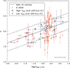 |
Fig. 11. Distribution of the X-HESS AGNs in the Γ − log λEdd, O/UV plane. Orange circles represent the X-HESS AGNs with available OM data and, for those disposing of multi-epoch observations, we considered their high-flux state. Low-λEdd and high-λEdd local AGNs from Liu et al. (2021) are shown as well with blue squares and red triangles, respectively. The average error on log λEdd, O/UV for the X-HESS AGNs is reported in the lower right corner. |
Following the same approach described in Sect. 4.2, we calculated the best-fit relation by adopting a bootstrapping method. In this way, we now obtain

which is approximately consistent with that in Eq. (2) and has a 1σ spread of about ∼0.26. If we considered only the highest flux state for the multi-epoch X-HESS AGNs in Fig. 11, we would obtain a similar best-fit relation, whose slope and intercept are 0.21 ± 0.04 and 2.13 ± 0.03, respectively. In this case, the 1σ spread is clearly smaller and amounts to ∼0.22.
For completeness, when dealing with the Γ − λEdd relation, we should also mention that according to recent studies, the size of the AGN broad line region calculated from the radius-luminosity relation could be significantly overestimated, affecting the MBH measurements in the same way (e.g. Du & Wang 2019; GRAVITY Collaboration 2024). Moreover, in the high-λEdd regime, provided that the slim disc model represents a reliable description of the inner accretion flow, the optical-based Lbol measurements may be underestimated (e.g. Castelló-Mor et al. 2016) or, at worst, not even represent the actual accretion power due to the photon-trapping effect.
Both of these effects, when combined, might cause an overall shift in the distribution in the Γ − λEdd plane towards higher λEdd values. The best-fit relation could also be affected, though it is hard to quantify explicitly. In any case, the large spread of Γ values would remain unchanged.
5. Soft excess: The Γ − RS/P relation
As is discussed in Sect. 3.2, the best-fit results of our X-ray spectral analysis of the X-HESS AGNs suggest that their spectrum is characterised by an excess of soft X-ray emission that we observe in approximately ∼40% of the total number of observations. This can be attributed to the redshift distribution of the X-HESS AGNs, since ∼44% of the sample sources is located at z ≥ 1. This implies that the observed E = 0.5 − 2 keV range corresponds to rest-frame intervals from E = 1 keV upward, making the detection of the soft excess very difficult in this case. On the other hand, in the rest of the cases we find that ≳70% of the X-HESS AGNs at z < 1 is characterised by a soft excess. For all the observations of these sources, we can calculate the parameter 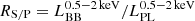 , which represents a proxy of the relative strength between the luminosity of the blackbody and power-law components (i.e. the soft excess and the primary continuum, respectively) in the E = 0.5 − 2 keV rest-frame energy band. The RS/P values of the X-HESS AGNs can be found in Table C.1.
Interestingly, we find evidence for a negative correlation between RS/P and the photon index, Γ, when we consider the first source in our X-HESS 1 sample; that is, SDSS J094610.71+095226.3, the X-HESS AGN with the largest number of available X-ray observations (15), each showing the presence of an excess of soft X-ray emission. This anti-correlation is significant according to Pearson, with a correlation coefficient of r = −0.81 for a null probability of p(> |r|) ∼ 2 × 10⁻⁴, while it is only marginally significant according to Spearman, with a correlation coefficient of ρS = −0.73 for a null probability of p(> |ρS|) ∼ 2 × 10⁻³.
When considered separately, each of the remaining X-HESS sources with a soft excess in their X-ray spectra dispose of less than half of the total observations of X-HESS 1, preventing us from recovering a similarly significant correlation between the two quantities. However, when we consider the entire fraction of X-HESS AGNs with an excess of soft X-ray emission – ∼40% of the complete sample discussed above – we find that Γ and RS/P appear to also be anti-correlated in this case, and the anti-correlation is mildly significant according to both Pearson and Spearman, with a correlation coefficient of r = −0.45 and ρS = −0.39 for a null probability of p(> |r|) ∼ 5 × 10⁻⁴ and p(> |ρS|) ∼ 3 × 10⁻³, respectively. However, the correlation coefficient does not account for the measurement errors, which, in turn, may provide a biased result. To overcome this issue, we adopted a bootstrapping method consisting of resampling the Γ and RS/P values of the X-HESS AGNs for N = 10 000 times, while accounting for the uncertainty on both quantities (see, e.g. Curran 2014). In this way, we obtain a distribution of ρS values and their corresponding null probabilities, whose median values provide a less biased estimator of the Spearman’s rank coefficient and p(> |ρS|). Specifically, we find ρS = −0.44 and p(> |ρS|) ∼ 7 × 10⁻⁴.
As the total number of observations of the X-HESS AGNs with a soft excess is approximately ∼60, we tried to determine a best-fit relation as follows. We adopted the BCES linear regression algorithm, since it takes into account the errors in both variables. Within the BCES family of models, we chose BCES x|y, which assumes y as the independent variable that, in our case, is represented by the slope of the power-law continuum, Γ. The resulting best-fit relation is

Figure 12 shows the best-fit relation based on the X-HESS AGNs and, for comparison, the samples of Palomar-Green (PG) QSOs by Piconcelli et al. (2005) and the high-λEdd AGNs analysed in Laurenti et al. (2022) are also included. The X-ray spectral analysis of X-HESS can be consistently compared with those of the other two samples, as they all share the same approach. By combining the measurements of high-λEdd AGNs from both Laurenti et al. (2022) and X-HESS, we obtain a similar relation; that is,
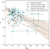 |
Fig. 12. Distribution of the X-HESS AGNs (in green) in the Γ − RS/P plane zoomed in on the region where RS/P ≤ 3.5. The sample of PG QSOs by Piconcelli et al. (2005) and the high-λEdd AGNs studied by Laurenti et al. (2022) are shown in brown and cyan, respectively. The dash-dotted black line indicates the best-fit relation for the PG QSOs. The solid black line describes the BCES x|y best-fit relation derived from the X-HESS AGNs, while the shaded area indicates the 90% confidence band. |

Moreover, the previous results are in partial agreement, within the uncertainties, with what we find for the sample of ∼40 PG QSOs of Piconcelli et al. (2005). Indeed, by adopting a simple weighted least squares model to fit the data points, we obtain

However, the above relation is only marginally significant according to Pearson, with a correlation coefficient of r = −0.47 for a null probability of p(> |r|) ∼ 4 × 10⁻³.
When we consider the three samples of Fig. 12 altogether, we get additional evidence for the existence of a significant negative correlation between Γ and RS/P, the correlation coefficients being r = −0.49 and ρS = −0.39 for a null probability of p(> |r|) ∼ 4 × 10⁻⁵ and p(> |ρS|) ∼ 10−3 according to Pearson and Spearman, respectively. Although the correlation is only mildly significant, it provides at least an indication of the possible existence of a relation between the two quantities.
Interestingly, this result appears to move in the opposite direction compared to previous findings, which suggested a putative positive correlation between the photon index and the strength of the soft excess (e.g. Bianchi et al. 2009; Boissay et al. 2016; Gliozzi & Williams 2020). However, except for Bianchi et al. (2009) and one of the three indicators in Gliozzi & Williams (2020), the reported correlations are only marginally significant. Although the different results may be partially affected by different models, it would be tempting to associate this trend with the high-λEdd nature of our AGNs, since all of the studies mentioned above contained a limited number of highly accreting AGNs. Despite the physical origin of the soft excess being still debated, three main competing scenarios are generally hypothesised nowadays. In the first, the soft excess arises from the enhancement of reflection from the inner regions of the accretion disc due to light-bending effects, together with a strong suppression of the primary emission (e.g. Miniutti & Fabian 2004). The second scenario is based on the assumption that the soft excess can also be mimicked by absorption from a relativistically outflowing warm gas (e.g. Gierliński & Done 2004). Finally, according to the third scenario, the observed excess of soft X-ray emission may be a signature of the high-energy tail of thermal Comptonisation in a warm (kT ∼ 1 keV), optically thick (τ ∼ 10 − 20) corona (e.g. Petrucci et al. 2018, and references therein).
If the soft excess is due to reflection from an ionised disc, a negative correlation is expected between the photon index and the strength of the soft excess (Boissay et al. 2016), in agreement with the indication that we get for the X-HESS AGNs. However, the modest S/N of some of the X-HESS observations does not allow us to constrain the properties of a putative reflection component to be included in our best-fit model.
On the other hand, we do not find any clear evidence of reflection features even in the higher-quality X-HESS spectra. Moreover, for the X-HESS AGNs, we obtain that the optical/UV luminosity at 2500 Å and the one in the soft X-rays are highly correlated (ρS = 0.84, p(> |ρS|) < 10−20). This would move in favour of a warm Comptonisation scenario, in which a strong link is expected between optical/UV and soft X-rays (e.g. Mehdipour et al. 2011), as the warm corona would lie above the surface of the inner accretion disc (Petrucci et al. 2020). In this case, however, we would have likely obtained a positive correlation between Γ and the soft excess strength, RS/P, at least if the warm corona efficiently provides the hot corona with the bulk of soft X-ray seed photons (Boissay et al. 2016). All this makes a really challenging task to shed definitive light on the origin of the Γ − RS/P relation. For the time being, our limited understanding of the interplay between the warm and hot coronae, as well as possibly different configurations and physical processes occurring in the warm corona, do not allow us to categorically rule out that the distribution in Fig. 12 could be also reproduced in this scenario.
In any case, higher-quality dedicated observations, especially extending towards the hard (E > 10 keV) X-rays, where one can find the typical spectral imprints due to reflection, are mandatory to quantify the hypothetical impact of ionised reflection in the X-HESS sample.
6. Summary and conclusions
In this paper, we have analysed a large new sample of high-λEdd AGNs named the XMM-Newton High-Eddington Serendipitous AGN Sample, or X-HESS, obtained by cross-correlating the 11th release of the XMM-Newton serendipitous catalogue and the catalogue of spectral properties of QSOs from Rakshit et al. (2020), according to the procedure described in Sect. 2. X-HESS contains 142 observations of 61 AGNs, and 22 of these highly accreting AGNs (∼36% of the sample sources) have been observed at different epochs by XMM-Newton for a total of 103 times. The X-HESS AGNs are distributed over wide intervals of bolometric luminosity (44.7 < log(Lbol/erg s−1) < 48.3), black hole mass (6.8 < log(MBH/M⊙) < 9.8), redshift (0.06 < z < 3.3), and the Eddington ratio (−0.2 < log λEdd < 0.5). Furthermore, a sizeable fraction of the X-HESS sources (∼62%) can rely on simultaneous OM observations obtained by cross-matching X-HESS with the latest release of the XMM-OM serendipitous catalogue. The main results of the analysis of the X-HESS sample can be summarised as follows.
-
The multi-epoch data coverage of a large fraction of the X-HESS AGNs allows us to investigate their spectral variability across the different observations in Sect. 4.1. Specifically, we considered the observations associated with their lowest- and highest-flux states, respectively. The latter, especially, are also particularly interesting for their implications in the often debated Γ − log λEdd relation. We do find that eight out of the 22 multi-epoch AGNs in X-HESS present significant spectral variations at the 1σ confidence level. The bulk of these AGNs appear to vary accordingly to a softer-when-brighter trend, whereas a single AGN follows the opposite trend. Moreover, such spectral variations do not exhibit a clear correlation with the time elapsed between the two observations of interest, which ranges from a few hours to ∼15 years (see Fig. 7).
-
A couple of X-HESS AGNs – namely, X-HESS 5 (z = 1.929) and 16 (z = 0.307) – have experienced at least one transition between phases of standard-to-weak X-ray emission (see Fig. 6). The observed transitions occur over very different timescales in the source’s rest-frame; approximately a week for the former and one and a half years for the latter. In both cases, we observe a drop in the soft and hard X-ray emission when moving from high- to low-flux states, leading to an overall hardening of the X-ray continuum. However, when accounting for the measurement errors, the corresponding spectral changes are only moderately or not at all significant for X-HESS 16 and 5, respectively. Moreover, their X-ray weak states do not appear to be due to absorption from intervening cold gas clouds.
-
We do not find a significant correlation between the X-ray photon index, Γ, and λEdd for the X-HESS AGNs, as is discussed in Sect. 4.2. Not only does this result hold when accounting for (or averaging) all the flux states of the multi-epoch X-HESS AGNs, but even when we considered, where available, the sole highest-flux state of each of these AGNs as the most representative of their X-ray coronal emission, in case some hypothetical degree of obscuration is present, though mostly undetected in our case, possibly due to limited S/N observations. This approach is shared by other authors, such as Liu et al. (2021), who studied a sample of 47 local AGNs located at z ≲ 0.3 and divided into two groups consisting of 21 high-λEdd and 26 low-λEdd sources with MBH measurements from reverberation mapping. These AGNs are mainly characterised by lower black hole masses compared to X-HESS. If we consider the X-HESS and high-λEdd local AGN from Liu et al. (2021), we still cannot find any significant correlation between Γ and λEdd in a relatively broad interval of Eddington ratios spanning from ∼ − 1 up to ≳0.7. On the other hand, when we consider X-HESS and both the local Liu et al. (2021) AGN samples, we obtain a highly significant correlation between the two quantities. In any case, the distribution in the Γ − log λEdd plane is affected by a very large spread.
-
We have investigated the possible effects of the black hole mass and bolometric luminosity in the observed Γ − log λEdd plane and found that the correlation between the photon index and the Eddington ratio is much more significant for those sources with either lower Lbol or MBH, while it basically becomes insignificant for AGNs with a higher black hole mass and/or bolometric luminosity. Results from partial correlation analysis in Sect. 4.3 appear to confirm this trend and possibly suggest that such a different behaviour in the Γ − log λEdd plane could likely reflect intrinsic differences between these two classes of objects, which approximately resemble the properties of local Seyfert-like galaxies and moderate-to-high-redshift QSOs, respectively.
-
We find that the use of simultaneous optical/UV observations, such as those provided by XMM-Newton, can offer the unprecedented possibility of obtaining measurements of the Eddington ratio, λEdd, O/UV, at different epochs by adopting the bolometric correction in Duras et al. (2020), as is described in Sect. 4.4. This is particularly important because it allows us to take a snapshot of the actual flux state of the given AGN, which may differ from that associated with the single-epoch spectrum used to determine λEdd. Thanks to this approach, we re-projected the Γ − log λEdd plane into its fully epoch-dependent variant, where both Γ and λEdd, O/UV represent a proxy of the ongoing AGN activity (see Fig. 11). By considering the X-HESS AGNs and both the local AGN samples from Liu et al. (2021), we find that Γ and λEdd, O/UV are statistically correlated and share an approximately similar spread around the best-fit relation compared to what previously found for the ‘standard’ single-epoch λEdd estimates. In both cases, due to the large scatter in the corresponding planes, we warmly recommend caution when using this relation to estimate the black hole mass. However, ideally, the adoption of a fully epoch-dependent approach would likely represent the fairest description of the actual distribution in the Γ − λEdd plane. Furthermore, this result shows the crucial importance for the X-ray observatories of collecting simultaneous optical/UV data, as in the case of XMM-Newton or Swift, to assess the time-dependent accretion properties of AGNs.
-
Approximately ∼40% of the total observations of the X-HESS AGNs, corresponding to ≳70% of all the AGNs at z < 1 for which the rest-frame E = 0.5 − 2 keV interval is broadly visible, indicates the presence of an excess of soft X-ray emission that we modelled with a blackbody component to provide a phenomenological description. For all these observations, we calculated the parameter
 , which quantifies the relative strength of the soft excess with respect to the underlying power-law continuum in the E = 0.5 − 2 keV observer-frame energy band. We get a mild indication of a negative correlation between RS/P and the photon index, Γ, when we consider the AGN with the largest number of observations – X-HESS 1 – as well as when we consider the whole subsample of X-HESS AGNs characterised by a soft excess (see Sect. 5). This result still holds if we consider the X-HESS sources and the AGNs in the Piconcelli et al. (2005) and Laurenti et al. (2022) samples altogether. Interestingly, according to Boissay et al. (2016), a similar anti-correlation is expected if the soft excess is due to reflection from an ionised disc.
In the near future, we plan to update X-HESS with more recent releases of the XMM-Newton serendipitous catalogue, which has recently reached its fourteenth version (4XMM-DR145), to increase the number of high-λEdd AGNs in the X-HESS sample and their corresponding observations. To this extent, we also note that, given the relatively bright E = 0.5 − 2 keV fluxes of the X-HESS AGNs, we can expect that the vast majority of our highly accreting AGNs will be detected by eROSITA.
Finally, in order to test any physical scenario to explain the observed properties of high-λEdd AGNs, it would be necessary to expand their study by adopting a multi-wavelength treatment. This is particularly feasible in the optical/UV band, where a large number of facilities, such as ZTF and Pan-STARRS, are continuously collecting photometric data in multiple wavelengths. Specifically, a major leap in this quest will be provided by the forthcoming Rubin Observatory Legacy Survey of Space and Time (LSST; Ivezić et al. 2019), which is expected to be fully operational in 2024. The unprecedented quality of LSST photometry will hopefully allow us, for example, to probe whether the slim disc, likely originating in highly accreting AGNs, presents peculiar optical/UV emission properties with respect to AGNs accreting in the low-to-moderate regime, and compare the X-ray and optical/UV characteristic flux variability to test different competing scenarios envisaging the presence (or lack) of correlated variations between the two bands.
Data availability
Tables A.1, B.1 and C.1 are available at the CDS via anonymous ftp to cdsarc.cds.unistra.fr (130.79.128.5) or via https://cdsarc.cds.unistra.fr/viz-bin/cat/J/A+A/689/A337
Acknowledgments
We thank the anonymous referee for the useful comments that helped us improve our manuscript. This work is based on observations obtained with XMM-Newton, an ESA science mission with instruments and contributions directly funded by ESA member states and the USA (NASA). ML is thankful to ESA, as part of this work has been carried out at ESA-ESTEC in the context of the Archival Research Visitor Programme 2021. ML, FT and EP acknowledge funding from the European Union – Next Generation EU, PRIN/MUR 2022 (2022K9N5B4). EP acknowledges support from PRIN MIUR project “Black Hole winds and the Baryon Life Cycle of Galaxies: the stone-guest at the galaxy evolution supper”, contract no. 2017PH3WAT. EP and LZ acknowledge financial support from the Bando Ricerca Fondamentale INAF 2022 Large Grant “Toward an holistic view of the Titans: multi-band observations of z > 6 QSOs powered by greedy supermassive black-holes”.
References
- Abramowicz, M. A., Czerny, B., Lasota, J. P., & Szuszkiewicz, E. 1988, ApJ, 332, 646 [Google Scholar]
- Ai, Y. L., Yuan, W., Zhou, H. Y., Wang, T. G., & Zhang, S. H. 2011, ApJ, 727, 31 [NASA ADS] [CrossRef] [Google Scholar]
- Arnaud, K. A. 1996, ASP Conf. Ser., 101, 17 [Google Scholar]
- Avni, Y. 1976, ApJ, 210, 642 [NASA ADS] [CrossRef] [Google Scholar]
- Bañados, E., Venemans, B. P., Decarli, R., et al. 2016, ApJS, 227, 11 [Google Scholar]
- Baskin, A., & Laor, A. 2005, MNRAS, 356, 1029 [NASA ADS] [CrossRef] [Google Scholar]
- Begelman, M. C., Volonteri, M., & Rees, M. J. 2006, MNRAS, 370, 289 [NASA ADS] [CrossRef] [Google Scholar]
- Bellm, E. C., Kulkarni, S. R., Graham, M. J., et al. 2019, PASP, 131, 018002 [Google Scholar]
- Bianchi, S., Guainazzi, M., Matt, G., Fonseca Bonilla, N., & Ponti, G. 2009, A&A, 495, 421 [NASA ADS] [CrossRef] [EDP Sciences] [Google Scholar]
- Bischetti, M., Piconcelli, E., Vietri, G., et al. 2017, A&A, 598, A122 [NASA ADS] [CrossRef] [EDP Sciences] [Google Scholar]
- Bischetti, M., Piconcelli, E., Feruglio, C., et al. 2019, A&A, 628, A118 [NASA ADS] [CrossRef] [EDP Sciences] [Google Scholar]
- Boissay, R., Ricci, C., & Paltani, S. 2016, A&A, 588, A70 [NASA ADS] [CrossRef] [EDP Sciences] [Google Scholar]
- Bongiorno, A., Zamorani, G., Gavignaud, I., et al. 2007, A&A, 472, 443 [NASA ADS] [CrossRef] [EDP Sciences] [Google Scholar]
- Brandt, W. N., Mathur, S., & Elvis, M. 1997, MNRAS, 285, L25 [NASA ADS] [CrossRef] [Google Scholar]
- Brightman, M., Silverman, J. D., Mainieri, V., et al. 2013, MNRAS, 433, 2485 [Google Scholar]
- Cackett, E. M., Gelbord, J., Li, Y.-R., et al. 2020, ApJ, 896, 1 [NASA ADS] [CrossRef] [Google Scholar]
- Cash, W. 1979, ApJ, 228, 939 [Google Scholar]
- Castelló-Mor, N., Netzer, H., & Kaspi, S. 2016, MNRAS, 458, 1839 [CrossRef] [Google Scholar]
- Castelló-Mor, N., Kaspi, S., Netzer, H., et al. 2017, MNRAS, 467, 1209 [NASA ADS] [Google Scholar]
- Chen, L.-H., & Wang, J.-M. 2004, ApJ, 614, 101 [NASA ADS] [CrossRef] [Google Scholar]
- Coatman, L., Hewett, P. C., Banerji, M., et al. 2017, MNRAS, 465, 2120 [Google Scholar]
- Costantini, E., Gallo, L. C., Brandt, W. N., Fabian, A. C., & Boller, T. 2007, MNRAS, 378, 873 [NASA ADS] [CrossRef] [Google Scholar]
- Curran, P. A. 2014, ArXiv e-prints [arXiv:1411.3816] [Google Scholar]
- Donnan, F. R., Hernández Santisteban, J. V., Horne, K., et al. 2023, MNRAS, 523, 545 [NASA ADS] [CrossRef] [Google Scholar]
- Du, P., & Wang, J.-M. 2019, ApJ, 886, 42 [NASA ADS] [CrossRef] [Google Scholar]
- Duras, F., Bongiorno, A., Ricci, F., et al. 2020, A&A, 636, A73 [NASA ADS] [CrossRef] [EDP Sciences] [Google Scholar]
- Fabian, A. C., Kara, E., Walton, D. J., et al. 2013, MNRAS, 429, 2917 [NASA ADS] [CrossRef] [Google Scholar]
- Ferrarese, L., & Merritt, D. 2000, ApJ, 539, L9 [Google Scholar]
- Fitzpatrick, E. L. 1999, PASP, 111, 63 [Google Scholar]
- Fukumura, K., Hendry, D., Clark, P., Tombesi, F., & Takahashi, M. 2016, ApJ, 827, 31 [NASA ADS] [CrossRef] [Google Scholar]
- Gallerani, S., Maiolino, R., Juarez, Y., et al. 2010, A&A, 523, A85 [NASA ADS] [CrossRef] [EDP Sciences] [Google Scholar]
- Gallo, L. C. 2006, MNRAS, 368, 479 [NASA ADS] [Google Scholar]
- Gibson, R. R., & Brandt, W. N. 2012, ApJ, 746, 54 [NASA ADS] [CrossRef] [Google Scholar]
- Gierliński, M., & Done, C. 2004, MNRAS, 349, L7 [Google Scholar]
- Gliozzi, M., & Williams, J. K. 2020, MNRAS, 491, 532 [Google Scholar]
- GRAVITY Collaboration (Amorim, A., et al.) 2024, A&A, 684, A167 [NASA ADS] [CrossRef] [EDP Sciences] [Google Scholar]
- Hopkins, P. F., Strauss, M. A., Hall, P. B., et al. 2004, AJ, 128, 1112 [Google Scholar]
- Huang, J., Luo, B., Du, P., et al. 2020, ApJ, 895, 114 [NASA ADS] [CrossRef] [Google Scholar]
- Ighina, L., Belladitta, S., Caccianiga, A., et al. 2021, A&A, 647, L11 [NASA ADS] [CrossRef] [EDP Sciences] [Google Scholar]
- Inayoshi, K., Haiman, Z., & Ostriker, J. P. 2016, MNRAS, 459, 3738 [NASA ADS] [CrossRef] [Google Scholar]
- Ivezić, Ž., Kahn, S. M., Tyson, J. A., et al. 2019, ApJ, 873, 111 [Google Scholar]
- Jansen, F., Lumb, D., Altieri, B., et al. 2001, A&A, 365, L1 [NASA ADS] [CrossRef] [EDP Sciences] [Google Scholar]
- Jin, C., Ward, M., & Done, C. 2012, MNRAS, 425, 907 [NASA ADS] [CrossRef] [Google Scholar]
- Jin, C., Done, C., Middleton, M., & Ward, M. 2013, MNRAS, 436, 3173 [NASA ADS] [CrossRef] [Google Scholar]
- Kaiser, N., Aussel, H., Burke, B. E., et al. 2002, SPIE Conf. Ser., 4836, 154 [Google Scholar]
- Kamizasa, N., Terashima, Y., & Awaki, H. 2012, ApJ, 751, 39 [NASA ADS] [CrossRef] [Google Scholar]
- Kamraj, N., Brightman, M., Harrison, F. A., et al. 2022, ApJ, 927, 42 [NASA ADS] [CrossRef] [Google Scholar]
- Kawamuro, T., Ueda, Y., Tazaki, F., Ricci, C., & Terashima, Y. 2016, ApJS, 225, 14 [NASA ADS] [CrossRef] [Google Scholar]
- King, A., & Pounds, K. 2015, ARA&A, 53, 115 [NASA ADS] [CrossRef] [Google Scholar]
- Krawczyk, C. M., Richards, G. T., Gallagher, S. C., et al. 2015, AJ, 149, 203 [NASA ADS] [CrossRef] [Google Scholar]
- Laurenti, M., Luminari, A., Tombesi, F., et al. 2021, A&A, 645, A118 [NASA ADS] [CrossRef] [EDP Sciences] [Google Scholar]
- Laurenti, M., Piconcelli, E., Zappacosta, L., et al. 2022, A&A, 657, A57 [NASA ADS] [CrossRef] [EDP Sciences] [Google Scholar]
- Liu, Z., Merloni, A., Georgakakis, A., et al. 2016, MNRAS, 459, 1602 [Google Scholar]
- Liu, H., Luo, B., Brandt, W. N., et al. 2021, ApJ, 910, 103 [Google Scholar]
- Lu, K.-X., Huang, Y.-K., Zhang, Z.-X., et al. 2019, ApJ, 877, 23 [NASA ADS] [CrossRef] [Google Scholar]
- Luminari, A., Nicastro, F., Elvis, M., et al. 2021, A&A, 646, A111 [NASA ADS] [CrossRef] [EDP Sciences] [Google Scholar]
- Lusso, E., Comastri, A., Vignali, C., et al. 2010, A&A, 512, A34 [NASA ADS] [CrossRef] [EDP Sciences] [Google Scholar]
- Lusso, E., Valiante, R., & Vito, F. 2023, in Handbook of X-ray and Gamma-ray Astrophysics, eds. C. Bambi, & A. Santangelo, 122 [Google Scholar]
- Mainzer, A., Bauer, J., Grav, T., et al. 2011, ApJ, 731, 53 [Google Scholar]
- Martocchia, S., Piconcelli, E., Zappacosta, L., et al. 2017, A&A, 608, A51 [NASA ADS] [CrossRef] [EDP Sciences] [Google Scholar]
- Marziani, P., & Sulentic, J. W. 2014, MNRAS, 442, 1211 [NASA ADS] [CrossRef] [Google Scholar]
- Marziani, P., Martínez Carballo, M. A., Sulentic, J. W., et al. 2016, Ap&SS, 361, 29 [NASA ADS] [CrossRef] [Google Scholar]
- Marziani, P., del Olmo, A., D’Onofrio, M., et al. 2018, Revisiting Narrow-Line Seyfert 1 Galaxies and their Place in the Universe, 2 [Google Scholar]
- Mason, K. O., Breeveld, A., Much, R., et al. 2001, A&A, 365, L36 [NASA ADS] [CrossRef] [EDP Sciences] [Google Scholar]
- Mateos, S., Saxton, R. D., Read, A. M., & Sembay, S. 2009, A&A, 496, 879 [NASA ADS] [CrossRef] [EDP Sciences] [Google Scholar]
- Mazzucchelli, C., Bañados, E., Venemans, B. P., et al. 2017, ApJ, 849, 91 [Google Scholar]
- Mehdipour, M., Branduardi-Raymont, G., Kaastra, J. S., et al. 2011, A&A, 534, A39 [NASA ADS] [CrossRef] [EDP Sciences] [Google Scholar]
- Middei, R., Petrucci, P. O., Bianchi, S., et al. 2020, A&A, 640, A99 [NASA ADS] [CrossRef] [EDP Sciences] [Google Scholar]
- Middei, R., Nardini, E., Matzeu, G. A., et al. 2023, A&A, 680, A50 [NASA ADS] [CrossRef] [EDP Sciences] [Google Scholar]
- Mineshige, S., Kawaguchi, T., Takeuchi, M., & Hayashida, K. 2000, PASJ, 52, 499 [NASA ADS] [CrossRef] [Google Scholar]
- Miniutti, G., & Fabian, A. C. 2004, MNRAS, 349, 1435 [NASA ADS] [CrossRef] [Google Scholar]
- Nandra, K., & Pounds, K. A. 1994, MNRAS, 268, 405 [Google Scholar]
- Nardini, E., Reeves, J. N., Gofford, J., et al. 2015, Science, 347, 860 [Google Scholar]
- Nardini, E., Lusso, E., Risaliti, G., et al. 2019, A&A, 632, A109 [NASA ADS] [CrossRef] [EDP Sciences] [Google Scholar]
- Onoue, M., Bañados, E., Mazzucchelli, C., et al. 2020, ApJ, 898, 105 [Google Scholar]
- Osterbrock, D. E., & Pogge, R. W. 1985, ApJ, 297, 166 [Google Scholar]
- Page, M. J., Brindle, C., Talavera, A., et al. 2012, MNRAS, 426, 903 [NASA ADS] [CrossRef] [Google Scholar]
- Paolillo, M., Schreier, E. J., Giacconi, R., Koekemoer, A. M., & Grogin, N. A. 2004, ApJ, 611, 93 [NASA ADS] [CrossRef] [Google Scholar]
- Pâris, I., Petitjean, P., Aubourg, É., et al. 2018, A&A, 613, A51 [Google Scholar]
- Petrucci, P. O., Ursini, F., De Rosa, A., et al. 2018, A&A, 611, A59 [NASA ADS] [CrossRef] [EDP Sciences] [Google Scholar]
- Petrucci, P. O., Gronkiewicz, D., Rozanska, A., et al. 2020, A&A, 634, A85 [NASA ADS] [CrossRef] [EDP Sciences] [Google Scholar]
- Piconcelli, E., Jimenez-Bailón, E., Guainazzi, M., et al. 2005, A&A, 432, 15 [NASA ADS] [CrossRef] [EDP Sciences] [Google Scholar]
- Prevot, M. L., Lequeux, J., Maurice, E., Prevot, L., & Rocca-Volmerange, B. 1984, A&A, 132, 389 [Google Scholar]
- Proga, D. 2005, ApJ, 630, L9 [NASA ADS] [CrossRef] [Google Scholar]
- Pu, X., Luo, B., Brandt, W. N., et al. 2020, ApJ, 900, 141 [Google Scholar]
- Rakshit, S., Stalin, C. S., & Kotilainen, J. 2020, ApJS, 249, 17 [Google Scholar]
- Read, A. M., Rosen, S. R., Saxton, R. D., & Ramirez, J. 2011, A&A, 534, A34 [NASA ADS] [CrossRef] [EDP Sciences] [Google Scholar]
- Read, A. M., Guainazzi, M., & Sembay, S. 2014, A&A, 564, A75 [NASA ADS] [CrossRef] [EDP Sciences] [Google Scholar]
- Reeves, J. N., O’Brien, P. T., Braito, V., et al. 2009, ApJ, 701, 493 [NASA ADS] [CrossRef] [Google Scholar]
- Ricci, C., Ho, L. C., Fabian, A. C., et al. 2018, MNRAS, 480, 1819 [NASA ADS] [CrossRef] [Google Scholar]
- Richards, G. T., Hall, P. B., Vanden Berk, D. E., et al. 2003, AJ, 126, 1131 [Google Scholar]
- Richards, G. T., Lacy, M., Storrie-Lombardi, L. J., et al. 2006, ApJS, 166, 470 [Google Scholar]
- Risaliti, G., Young, M., & Elvis, M. 2009, ApJ, 700, L6 [NASA ADS] [CrossRef] [Google Scholar]
- Schlafly, E. F., & Finkbeiner, D. P. 2011, ApJ, 737, 103 [Google Scholar]
- Serafinelli, R., Vagnetti, F., & Middei, R. 2017, A&A, 600, A101 [NASA ADS] [CrossRef] [EDP Sciences] [Google Scholar]
- Shakura, N. I., & Sunyaev, R. A. 1973, A&A, 24, 337 [NASA ADS] [Google Scholar]
- Shankar, F., Weinberg, D. H., & Miralda-Escudé, J. 2013, MNRAS, 428, 421 [NASA ADS] [CrossRef] [Google Scholar]
- Shemmer, O., Brandt, W. N., Netzer, H., Maiolino, R., & Kaspi, S. 2006, ApJ, 646, L29 [Google Scholar]
- Shemmer, O., Brandt, W. N., Netzer, H., Maiolino, R., & Kaspi, S. 2008, ApJ, 682, 81 [Google Scholar]
- Shirakata, H., Kawaguchi, T., Oogi, T., Okamoto, T., & Nagashima, M. 2019, MNRAS, 487, 409 [NASA ADS] [CrossRef] [Google Scholar]
- Sądowski, A., Abramowicz, M., Bursa, M., et al. 2011, A&A, 527, A17 [NASA ADS] [CrossRef] [EDP Sciences] [Google Scholar]
- Sobolewska, M. A., & Done, C. 2007, MNRAS, 374, 150 [NASA ADS] [CrossRef] [Google Scholar]
- Sobolewska, M. A., & Papadakis, I. E. 2009, MNRAS, 399, 1597 [NASA ADS] [CrossRef] [Google Scholar]
- Soldi, S., Beckmann, V., Baumgartner, W. H., et al. 2014, A&A, 563, A57 [NASA ADS] [CrossRef] [EDP Sciences] [Google Scholar]
- Strüder, L., Briel, U., Dennerl, K., et al. 2001, A&A, 365, L18 [Google Scholar]
- Tombesi, F., Meléndez, M., Veilleux, S., et al. 2015, Nature, 519, 436 [NASA ADS] [CrossRef] [Google Scholar]
- Trakhtenbrot, B., Ricci, C., Koss, M. J., et al. 2017, MNRAS, 470, 800 [NASA ADS] [CrossRef] [Google Scholar]
- Trefoloni, B., Lusso, E., Nardini, E., et al. 2023, A&A, 677, A111 [NASA ADS] [CrossRef] [EDP Sciences] [Google Scholar]
- Turner, M. J. L., Abbey, A., Arnaud, M., et al. 2001, A&A, 365, L27 [CrossRef] [EDP Sciences] [Google Scholar]
- Vagnetti, F., Turriziani, S., Trevese, D., & Antonucci, M. 2010, A&A, 519, A17 [NASA ADS] [CrossRef] [EDP Sciences] [Google Scholar]
- Vagnetti, F., Antonucci, M., & Trevese, D. 2013, A&A, 550, A71 [NASA ADS] [CrossRef] [EDP Sciences] [Google Scholar]
- Vagnetti, F., Middei, R., Antonucci, M., Paolillo, M., & Serafinelli, R. 2016, A&A, 593, A55 [NASA ADS] [CrossRef] [EDP Sciences] [Google Scholar]
- Valiante, R., Agarwal, B., Habouzit, M., & Pezzulli, E. 2017, PASA, 34, e031 [Google Scholar]
- Vanden Berk, D. E., Richards, G. T., Bauer, A., et al. 2001, AJ, 122, 549 [Google Scholar]
- Vietri, G., Piconcelli, E., Bischetti, M., et al. 2018, A&A, 617, A81 [NASA ADS] [CrossRef] [EDP Sciences] [Google Scholar]
- Vietri, G., Mainieri, V., Kakkad, D., et al. 2020, A&A, 644, A175 [NASA ADS] [CrossRef] [EDP Sciences] [Google Scholar]
- Wachter, K., Leach, R., & Kellogg, E. 1979, ApJ, 230, 274 [NASA ADS] [CrossRef] [Google Scholar]
- Waddell, S. G. H., & Gallo, L. C. 2020, MNRAS, 498, 5207 [NASA ADS] [CrossRef] [Google Scholar]
- Webb, N. A., Coriat, M., Traulsen, I., et al. 2020, A&A, 641, A136 [NASA ADS] [CrossRef] [EDP Sciences] [Google Scholar]
- Wu, X.-B., Wang, F., Fan, X., et al. 2015, Nature, 518, 512 [Google Scholar]
- Zappacosta, L., Piconcelli, E., Giustini, M., et al. 2020, A&A, 635, L5 [NASA ADS] [CrossRef] [EDP Sciences] [Google Scholar]
- Zhang, X., Lu, Y., & Fang, T. 2020, ApJ, 903, L18 [NASA ADS] [CrossRef] [Google Scholar]
- Zubovas, K., & King, A. 2012, ApJ, 745, L34 [Google Scholar]
- Zubovas, K., & King, A. 2013, ApJ, 769, 51 [NASA ADS] [CrossRef] [Google Scholar]
All Tables
Partial correlation analysis on the X-HESS and Liu et al. (2021) subsamples with either a lower or higher black hole mass and bolometric luminosity.
All Figures
|
Fig. 1. Distribution of the X-HESS AGNs in the log Lbol − log MBH plane (in black). Red squares indicate the high-λEdd local AGN subsample from Liu et al. (2021), as a comparison. With respect to this sample, the X-HESS AGNs extend towards larger values of both bolometric luminosity and black hole mass. Dash-dotted black lines describe different values of λEdd. |
| In the text | |
|
Fig. 2. Distribution of the X-HESS AGNs in the z − λEdd plane. All the X-HESS AGNs and the subsample with multi-epoch observations are described by grey dots and red diamonds, respectively. The multi-epoch subsample is well representative of the whole sample in terms of these quantities. |
| In the text | |
|
Fig. 3. Relative frequency histogram showing the distribution of the total net counts from EPIC-pn, MOS1, and MOS2 in the broad E = 0.3 − 10 keV observer-frame energy band for each individual observation of the X-HESS AGNs (in black). The distribution related to the observations with the largest number of counts of each X-HESS AGN is shown in purple. |
| In the text | |
|
Fig. 4. Pie chart describing the overall results of the spectroscopic analysis of the X-HESS sources. In most cases, the broadband X-ray continuum (E = 0.3 − 10 keV) can be reproduced well by a power-law model, modified by Galactic absorption. In the remaining ∼40% of the observations, an excess of soft X-ray emission is found. Approximately ∼12% of the X-ray spectra of the X-HESS AGNs reveal the presence of at least one emission and/or absorption feature due to the interaction of the primary continuum with either cold or ionised gas clouds. |
| In the text | |
|
Fig. 5. SDSS spectrum of J0234−08 (X-HESS 7) at z = 0.992 (in gold) compared to the composite QSO’s template of Vanden Berk et al. (2001). The template (in black) is extinguished according to the SMC extinction law by Prevot et al. (1984), with progressively increasing values of E(B − V). The value of E(B − V) that minimises the distance between the reddened template (in purple) and the observed SDSS spectrum at wavelengths of λobs < 8000 Å in the observer frame, corresponds to our estimate of the internal reddening of the source. J0234−08 has the largest E(B − V) among our sources, i.e. E(B − V) = 0.33. |
| In the text | |
|
Fig. 6. Distribution of the X-HESS AGNs in the αox − log LUV plane. Single- and multi-epoch AGNs are shown in grey and red, respectively. White circles with red edges highlight the high-flux state of the multi-epoch X-HESS AGNs. Solid and dashed black lines indicate the best-fit relation from Lusso et al. (2010) and the corresponding 1σ spread. The solid red line marks the reference value for X-ray weakness, i.e. Δαox ≤ −0.3 (Pu et al. 2020). Dotted and dash-dotted blue and green lines describe the time evolution of αox for the AGNs X-HESS 16 and X-HESS 5, respectively. Specifically, the latter has experienced a couple of transitions between phases of standard and weak X-ray emission over the different observations. |
| In the text | |
|
Fig. 7. Spectral variation in the photon index, Γ, versus the change in E = 2 − 10 keV X-ray luminosity between the lowest- and highest-flux states of the multi-epoch X-HESS AGNs. Luminosity changes of < 1% occurring within the red-hatched region are considered insignificant. Most of the sources vary accordingly to a softer-when-brighter trend, while a smaller fraction do the opposite. No clear correlation is found between the amplitude of the spectral variations and the time elapsed between the two observations of interest. |
| In the text | |
|
Fig. 8. Distribution of the X-HESS AGNs in the Γ − log λEdd plane. Single- and multi-epoch AGN are represented by grey circles and red diamonds, respectively. The best-fit relations from previous studies are reported as well. The average uncertainty on λEdd is 0.3 dex. |
| In the text | |
|
Fig. 9. Distribution of the X-HESS AGNs (orange circles) and the high-λEdd (blue squares) and low-λEdd local AGNs (red triangles) from Liu et al. (2021) in the Γ − log λEdd plane. For the multi-epoch X-HESS AGNs, we considered the Γ associated with their high-flux state. The black error bar in the lower right corner represents the average uncertainty on the X-HESS sources. Solid and dashed black lines describe the best-fit relation and its 1σ spread, respectively. The dash-dotted green line represents the Liu et al. (2021) best-fit relation, for comparison. |
| In the text | |
|
Fig. 10. Distribution of the X-HESS AGNs and the high-λEdd and low-λEdd local AGNs from Liu et al. (2021) in the Γ − log λEdd plane. All AGNs are divided in two almost equally populated sub-intervals of black hole mass (top panel) and bolometric luminosity (bottom panel). The correlation between Γ and λEdd appears to vanish for those sources with either higher MBH or Lbol. |
| In the text | |
|
Fig. 11. Distribution of the X-HESS AGNs in the Γ − log λEdd, O/UV plane. Orange circles represent the X-HESS AGNs with available OM data and, for those disposing of multi-epoch observations, we considered their high-flux state. Low-λEdd and high-λEdd local AGNs from Liu et al. (2021) are shown as well with blue squares and red triangles, respectively. The average error on log λEdd, O/UV for the X-HESS AGNs is reported in the lower right corner. |
| In the text | |
|
Fig. 12. Distribution of the X-HESS AGNs (in green) in the Γ − RS/P plane zoomed in on the region where RS/P ≤ 3.5. The sample of PG QSOs by Piconcelli et al. (2005) and the high-λEdd AGNs studied by Laurenti et al. (2022) are shown in brown and cyan, respectively. The dash-dotted black line indicates the best-fit relation for the PG QSOs. The solid black line describes the BCES x|y best-fit relation derived from the X-HESS AGNs, while the shaded area indicates the 90% confidence band. |
| In the text | |
Current usage metrics show cumulative count of Article Views (full-text article views including HTML views, PDF and ePub downloads, according to the available data) and Abstracts Views on Vision4Press platform.
Data correspond to usage on the plateform after 2015. The current usage metrics is available 48-96 hours after online publication and is updated daily on week days.
Initial download of the metrics may take a while.