| Issue |
A&A
Volume 699, July 2025
|
|
|---|---|---|
| Article Number | A202 | |
| Number of page(s) | 13 | |
| Section | Extragalactic astronomy | |
| DOI | https://doi.org/10.1051/0004-6361/202554433 | |
| Published online | 09 July 2025 | |
Measuring monster black hole masses: Maybe mighty, maybe merely massive
1
Department of Physics and Astronomy, George Mason University, 4400 University Drive, Fairfax, VA 22030, USA
2
Institute for Astronomy Astrophysics Space Applications and Remote Sensing (IAASARS), National Observatory of Athens, I. Metaxa & V. Pavlou, Penteli 15236, Greece
3
Physics Department, University of Crete, 73010 Heraklion, Greece
⋆ Corresponding author: This email address is being protected from spambots. You need JavaScript enabled to view it.
Received:
9
March
2025
Accepted:
7
June
2025
Abstract
Context. Accurate black hole mass (MBH) measurements in high-redshift galaxies are difficult yet crucial to constrain the growth of supermassive BHs, and to discriminate between competing BH seed models. Recent studies claimed the detection of massive BHs in very distant AGN, implying extreme conditions. However, these estimates are usually obtained by extrapolating indirect methods that are calibrated for moderately accreting, low-luminosity AGN in the local universe.
Aims. We want to assess the reliability of the single epoch method (SE) in the distant universe.
Methods. We computed the MBH values for a sample of hyperluminous distant quasars (the X-WISSH sample) and a sample of highly accreting AGN (X-HESS) using the X-ray scaling method.
Results. We first verified that the X-ray scaling method yields reliable MBH values also for distant highly accreting objects. Then, we carried out a systematic comparison with the SE method and found that these two indirect methods are fully consistent over a broad range of luminosities, intrinsic absorption, and accretion rates. The only discrepancies were associated with AGN that are substantially absorbed (underestimated by the SE method) and AGN accreting well above the Eddington limit (overestimated by the SE method). The latter result casts some doubts on the claim of overmassive BHs in highly accreting AGN in the early universe. Our study also reveals that one of the frequently used AGN catalogs consistently underestimates MBH by a factor of 2.5. Although this factor is on the order of the uncertainty associated with the SE method, we demonstrated that using these underestimated values can result in potentially misleading conclusions. Specifically, for this AGN sample we confirmed strong positive correlations for Γ versus λEdd, for the X-ray bolometric correction versus λEdd, and for Γ versus the soft excess strength, at odds with the conclusions inferred using underestimated MBH values.
Key words: accretion, accretion disks / black hole physics / galaxies: active / galaxies: high-redshift / X-rays: galaxies
© The Authors 2025
 Open Access article, published by EDP Sciences, under the terms of the Creative Commons Attribution License (https://creativecommons.org/licenses/by/4.0), which permits unrestricted use, distribution, and reproduction in any medium, provided the original work is properly cited.
This article is published in open access under the Subscribe to Open model. This email address is being protected from spambots. You need JavaScript enabled to view it. to support open access publication.
1. Introduction
It is now widely accepted that every massive galaxy hosts a supermassive black hole (SMBH) at its center, and that there exists a positive correlation between the mass of the BH (MBH) and that of the galaxy bulge, suggesting a coevolution between these two components (Magorrian et al. 1998; Ferrarese & Merritt 2000; Gebhardt et al. 2000).
Recent discoveries of quasars with MBH values on the order of 109−1010 M⊙ at redshifts of ∼7 (Mortlock et al. 2011; Venemans et al. 2013; Bañados et al. 2018; Fan et al. 2023) and, more recently, the advent of the James Webb Space Telescope (JWST) led to the detections of numerous galaxies at even larger redshifts, the so-called little red dots (LRDs), whose nature is still debated: they may be massive, compact star-forming galaxies (Labbé et al. 2023) or low-mass galaxies hosting moderately luminous active galactic nuclei (AGN) with overmassive BHs (Harikane et al. 2023; Maiolino et al. 2024). Importantly, very distant LRDs with estimated masses of SMBHs in the 106−108 M⊙ range (Larson et al. 2023; Matthee et al. 2024; Greene et al. 2024; Maiolino et al. 2024) impose severe constraints on current models looking for viable pathways of SMBH formation (see Regan & Volonteri 2024 for a recent review).
In principle, the detection of galaxies and SMBHs over a very large range of redshifts should make it possible to study the evolution of the relationship between these two components over cosmic time. However, accurate measurements of the SMBH mass and galaxy properties become very challenging at high redshifts. Here, we focus on the reliability of MBH measurements in distant AGN.
In nearby galaxies, where the BH sphere of influence is spatially resolved by current instrumentation, the MBH can be accurately estimated with direct methods by measuring the kinematics of the gas or stellar components in the inner region of weakly active galaxies (e.g., Macchetto et al. 1997; Gebhardt et al. 2003) or the kinematics of the broad line region (BLR) in nearby AGN (GRAVITY Collaboration 2018, 2021). For more distant AGN, which exhibit correlated variability between the optical-UV continuum emitted from the accretion disk and the line emission from the BLR, the MBH is accurately measured using the reverberation mapping (RM) technique (e.g., Blandford & McKee 1982; Peterson et al. 2004). However, this time- and instrument-intensive method is restricted to objects that vary substantially on a reasonably short time interval, limiting the direct measurements of MBH to moderately luminous nearby AGN.
For the vast majority of AGN, one must rely on indirect methods to estimate the MBH. For example, a positive correlation between MBH and the velocity dispersion of the galaxy bulge (the so-called M−σ★ correlation), observed in local nearly quiescent galaxies, is often utilized in cases where dynamical methods are not accessible (see Kormendy & Ho 2013 for a comprehensive review). This specific method, however, cannot be used for distant AGN for the following reasons: (1) there is evidence that AGN do not follow the M−σ★ correlation obtained using local inactive galaxies (Caglar et al. 2023); (2) the local M−σ★ correlation has a tendency to systematically overestimate MBH in AGN regardless of the level of obscuration (Gliozzi et al. 2024); (3) since the ultimate goal is to investigate the evolution of the correlation between BH and galaxy properties, one cannot use an MBH estimate inferred from this relationship.
Another indirect method, which is routinely applied to all type-1 AGN (that is, objects with detectable BLRs), is the single epoch (SE) method, which exploits the tight correlation observed between the size of the BLR RBLR and the optical luminosity Lopt (e.g., Kaspi et al. 2005; Bentz et al. 2013). The major advantage of the SE method is its ability to estimate MBH based on a single spectrum, which has led to the estimates of several thousands of MBH values at all redshifts utilizing large AGN spectral catalogs (e.g., Rakshit et al. 2020).
However, recent studies have outlined the tendency of this method to overestimate MBH when applied to highly accreting objects (see, e.g., Du et al. 2015, 2018; Martínez-Aldama et al. 2019) and to luminous AGN (Woo et al. 2024) since the method was calibrated using nearby, moderately accreting AGN with relatively low luminosities. Additional concerns about the reliability of the SE method applied to high-redshift AGN were cast by very recent studies from Bertemes et al. (2025), who demonstrated that different optical and UV broad lines can yield substantially different estimates of MBH for the same object, and by Fries et al. (2024), who performed a velocity-resolved reverberation mapping study of a highly variable quasar over a time interval of 10 years and revealed that the virial product (the basis of the SE method) was inconsistent over time.
Despite these concerns, the SE method often offers the only option to estimate MBH in distant AGN. Therefore, it is important to assess its reliability and its potential biases when applied to distant quasars and highly accreting AGN.
In our recent work, using a representative volume-limited sample of hard-X-ray-selected AGN, we carried out a systematic comparison of indirect methods to estimate MBH in all AGN regardless of their level of obscuration. Our analysis demonstrated that X-ray-based methods (specifically, the X-ray scaling method and the variability method based on the excess variance) yield MBH values that are fully consistent with those obtained with dynamical methods, whereas other methods such as the fundamental plane for black hole activity (e.g., Merloni et al. 2003; Gültekin et al. 2019) are either unreliable or have the tendency to overestimate MBH (for example, the M−σ★ correlation for inactive galaxies). Additionally, our study showed that, for broad-lined AGN, the X-ray-based methods were consistent with the SE method based on the Hα line (Gliozzi et al. 2024).
In principle, the X-ray-based methods could be extended to distant AGN without any substantial modification, but they may be affected by inherent difficulties. For example, the variability method (e.g., Papadakis 2004; Ponti et al. 2012; Akylas et al. 2022), which is model-independent and hence applicable to all variable AGN, is severely limited by the lack of light curves sufficiently long and with adequate signal-to-noise ratio. On the other hand, it is easier to obtain X-ray spectra of sufficient quality to apply the X-ray scaling method. This method is based on the assumption that the central engine (disk + corona) producing the X-rays works similarly in all black hole systems accreting at moderate or high rate (see Shaposhnikov & Titarchuk 2009; Gliozzi et al. 2011 for further details). This is supported by several studies on the similarities between AGN and stellar mass BHs (see, e.g., Done & Gierliński 2005; Körding et al. 2006; McHardy et al. 2006), as well as by the tight correlations observed between αox and L2500 Å (Steffen et al. 2006) and between the X-ray and UV luminosities (Risaliti & Lusso 2015), which appear to remain unchanged up to z = 6.
Nevertheless, since the X-ray scaling method, with the exception of the recent work from Elías-Chávez et al. (2024), has only been applied to relatively nearby AGN (Gliozzi et al. 2011, 2021, 2024; Giacchè et al. 2014; Seifina et al. 2018a, b; Shuvo et al. 2022; Williams et al. 2023), we first had to perform a sanity check and verify that it yields reasonable values also for distant objects. This was accomplished by comparing the MBH values obtained from this method with those of luminous quasars accreting at the Eddington level and with well-defined spectral energy distributions (SEDs). We then carried out a systematic comparison between the SE method and the X-ray scaling one using a large sample of highly accreting X-ray-bright AGN. Finally, we outlined the implications of using the X-ray-based MBH as opposed to values obtained with an automated analysis with the SE method by investigating different correlations between various AGN parameters.
The structure of the paper is as follows. In Section 2, we describe the sample selection, as well as the data reduction and analysis of the XMM-Newton data. In Section 3, we report the results obtained from the X-ray scaling method and the systematic comparison with the SE method. We discuss the main findings in Section 4 and draw our conclusions in Section 5. In this paper, we adopt a cosmology with H0 = 70 km s−1 Mpc−1, Ωm = 0.28, ΩΛ = 0.72, based on the 9-year measurements of the Wilkinson Microwave Anisotropy Probe (WMAP).
2. Observations
2.1. Description of the samples
In this study we utilized two different samples. First, we focused on the hyperluminous quasars of the WISSH sample, which contains objects with Lbol>2×1047 erg s−1 obtained from the cross-correlation of the WISE and SDSS catalogs (Bischetti et al. 2017). The X-ray properties of a subsample of 41 quasars, the X-WISSH sample, were studied by Martocchia et al. (2017). Of these quasars, 40 sources have MBH values estimated with the SE method based on the C IV line, and 14 have MBH values based on the Hβ line. Importantly, 35 of these quasars have broadband SEDs, which were used by Duras et al. (2020) to estimate the bolometric luminosity. Here, we restricted our work to 12 objects that have XMM-Newton spectral data of sufficient quality to constrain the main parameters of a Comptonization model, which are needed to estimate MBH with the X-ray scaling method. The basic characteristics of this sample of 12 WISSH quasars can be summarized as follows: the redshift z ranges from 2.04 to 4.11 with an average of 2.92, the bolometric luminosity is between 2.8×1047 erg s−1 and 5.0×1048 erg s−1 with an average of 1.0×1048 erg s−1, the 2−10 keV luminosity LX ranges from 1045 erg s−1 to 1.5×1046 erg s−1 with an average of 5.2×1045 erg s−1, and the Eddington ratio λEdd=Lbol/LEdd has minimum, maximum, and average of 0.08, 3.28, and 0.97, respectively. Throughout the paper, unless otherwise stated, the values of λEdd are computed assuming the MBH is obtained with the X-ray scaling method.
Second, we worked on the XMM-Newton High-Eddington Serendipitous AGN Sample (X-HESS), recently selected by Laurenti et al. (2024), which comprises 60 allegedly highly accreting objects with MBH estimated via the SE method with the Hβ line. Of these, we were able to estimate MBH for 50 objects with the X-ray scaling method. The main characteristics of this second sample are the following: z varies between 0.06 and 3.31 with an average of 1.09, Lbol ranges from 5×1044 erg s−1 to 2×1048 erg s−1 with an average of 2.9×1046 erg s−1, LX is between 4.6×1042 erg s−1 and 1.5×1046 erg s−1 with an average of 1.4×1045 erg s−1, and λEdd ranges between 0.01 and 9.7 with an average of 0.7. The main properties of the objects analyzed in this work are summarized in two tables in the appendix.
2.2. Data reduction
We processed the entire sample using the XMM-Newton pipeline spectral data products available in the XMM-Newton Science Archive (XSA) at the European Space Astronomy Centre (ESAC). The source spectrum was accumulated by using a spatial filter (a circular aperture whose radius was determined by an S/N optimization algorithm) on valid events in an exposure from CCDs operating in IMAGING mode. For each candidate source, a spectrum was produced for each EPIC camera (two MOS and one pn), where available. Additionally, for each source spectrum, a background spectrum was produced by accumulating detected events from a source-free region of the field of view (contaminating source regions having been masked out in the process). The corresponding ancillary response function file, which provides the effective area of the instrument as a function of energy, was also produced for each source and exposure for which spectral products have been extracted and was used with those spectral products.
2.3. X-ray spectral analysis
The X-ray scaling method is based on the spectral fitting of the primary X-ray emission of the objects in our sample with the bulk Comptonization model BMC (Titarchuk et al. 1997). To fit the hard X-ray spectrum where the lower energy limit is fixed at 2 keV in the source rest frame, we used a simple baseline model
constant*zphabs*BMC
where the constant takes into account the difference in calibration among the three XMM-Newton EPIC cameras, the absorption model zphabs describes both the Galaxy and the intrinsic contributions, and BMC parameterizes the Comptonization process. We performed the X-ray spectral analysis using the XSPEC v.12.9.0 software package (Arnaud 1996), and the errors quoted on the spectral parameters represent the 1σ confidence level.
3. Results
3.1. Black hole masses in the WISSH sample
To assess the validity of the SE method, we utilized the X-ray scaling method, which in principle is valid for any moderately to highly accreting BH system (we briefly summarize the main characteristics of this method in the appendix). However, one should bear in mind that this method is based on a simple Comptonization model (BMC), which was developed to study nearby objects. Therefore, we first had to test whether this X-ray-based method yields reasonable results also at high redshifts.
The X-WISSH sample offers the most direct way to test this hypothesis. By construction, this sample contains hyperluminous quasars, located at high redshifts, with broadband SEDs strongly dominated by the AGN component (Duras et al. 2020). It is reasonable to assume that these sources are accreting around the Eddington level (substantially lower accretion rates on the order of 0.1 would imply unrealistically high values of MBH on the order of 1011 M⊙ or more). Supporting this hypothesis are the considerably high values of the X-ray bolometric correction, KX=Lbol/LEdd, which, for the 12 sources analyzed here, ranges from 39 to 1066 with an average of 273, implying that these sources are X-ray weak, as expected for highly accreting objects. Additionally, Fig. 9 of Duras et al. (2020) shows the X-WISSH sample clusters around log(λEdd) = 0 in the KX−log(λEdd) plot. With this simple assumption, Lbol=Laccr=LEdd, we can derive reasonable estimates for the BH masses by using MBH,Edd=Lbol/(1.3×1038 erg s−1), which can then be compared with the values obtained with the X-ray scaling method.
The left panel of Fig. 1 shows that the masses computed with the X-ray scaling method MBH,X (plotted along the y-axis) are in general a good agreement with the MBH,Edd values. We quantified this apparent agreement using 〈max(MBH ratio)〉, which is the mean of the maximum value between MBH,X/MBH,Edd and MBH,Edd/MBH,X, and obtained 2.61 (with  , where n is the number of objects). We then iteratively decreased MBH,X using progressively smaller multiplicative factors to find a better agreement with MBH,Edd and found a marginal improvement (〈max(MBH ratio)〉 = 2.33,
  ) when using a multiplicative factor of 0.65, that is, when MBH,X is decreased by 35%, which is within the typical uncertainties of this method.
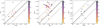 |
Fig. 1. Left panel: MBH obtained with the X-ray scaling method plotted vs. the values corresponding to sources accreting at the Eddington level. Middle panel: MBH obtained with the SE method using the C IV line plotted vs. the Eddington values. Right panel: MBH obtained with the SE method using the Hβ line plotted vs. the Eddington values. The symbols are color coded based on redshift. The continuous black line represents the one-to-one correlation and the dashed lines indicate departures by a factor of 3. |
When the same test is carried out on MBH values obtained from the SE method using the C IV line (illustrated in the middle panel of Fig. 1), it is evident that a sizable portion of the values is overestimated, confirming that these measurements have a tendency to yield unreliable estimates in highly accreting objects. Using the same diagnostic tool for the comparison between the values computed with the C IV line and the Eddington level MBH (35 objects have both measurements), we get 〈max(MBH ratio)〉 = 4.36.
On the other hand, the MBH estimates derived from the SE method using the Hβ line appear to be broadly consistent with the MBH,Edd values (right panel of Fig. 1). In this case (with only 11 objects), we get 〈max(MBH ratio)〉 = 1.82. Unfortunately, only three sources have MBH estimated with both the X-ray-based method and the Hβ-based SE method; therefore, it is not possible to assess the consistency between these two methods using this limited sample.
Since in this sample, there are only 12 and 11 objects with MBH determined with the X-ray method and with the SE method using the Hβ line, respectively, a statistical comparison with the corresponding Eddington limit values yields inconclusive results. Both sets of MBH values appear to be consistent with the Eddington ones according to a Kolmogorov-Smirnov test (PKS = 0.19 and 0.37, respectively), and their Spearman correlation coefficients indicate a positive but not statistically significant correlation with r = 0.40 (PS = 0.19) and r = 0.29 (PS = 0.38), respectively. On the other hand, the 35 sources with MBH determined via the C IV line make it possible to carry out a meaningful statistical comparison, which demonstrates that the distribution of these masses is not consistent with the Eddington limit one at high significance level (PKS = 7×10⁻⁷) and that there is a weak but not statistically significant positive correlation (r = 0.10, PS = 0.54).
In summary, exploiting the unique properties of the X-WISSH sample (highly accreting hyperluminous quasars with well-constrained bolometric luminosity and X-ray coverage), we can conclude that C IV-based SE measurements are an unreliable estimator of MBH, whereas both the X-ray scaling method and the Hβ-based SE method appear to yield reasonable results. Nevertheless, a larger sample of X-ray-bright, highly accreting AGN is necessary to carry out a quantitative comparison between these two indirect methods.
3.2. Black hole masses in the X-HESS sample
The X-HESS sample allows a direct comparison between the MBH estimates obtained with the X-ray scaling method and those derived with the SE method based mostly on the Hβ and Mg II lines. Of the original 60 AGN presented by Laurenti et al. (2024), 50 have adequate count rates and Γ in the proper range to apply the X-ray scaling method. A visual comparison between these two indirect methods is illustrated in Fig. 2, where the MBH values obtained from the SE method using different lines depending on the source redshift (specifically, 23 are based on the Hβ line and represented by circles, 25 on the Mg II line and illustrated with squares, and two on the C IV line and described by triangles) are plotted versus the values derived with the X-ray scaling method (the diamonds represent the four sources whose MBH values were flagged as unreliable in Rakshit et al. 2020). The figure has three panels with different color schemes illustrating, respectively: the redshift z (left panel), the intrinsic absorption measured by NH in units of 1022 cm−2 (middle panel), and the accretion rate level defined by log(λEdd) (right panel).
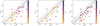 |
Fig. 2. Left panel: MBH obtained from the SE method using the Hβ line plotted vs. the values derived with the X-ray scaling method, with color-coded symbols indicating the redshift of the sources. Middle panel: Same as the left panel with color-coded symbols illustrating the intrinsic absorption NH in units of 1022 cm−2. Right panel: Same as the left panel with color-coded symbols describing the level of accretion rate, as defined by log(λEdd). Circles indicate MBH based on the Hβ line, squares are values based on the Mg II line, whereas the two triangles indicate the values based on the C IV line; the diamonds represent the sources whose MBH values were flagged as unreliable in Rakshit et al. (2020). |
A visual inspection of Fig. 2 clearly indicates the existence of a strong positive correlation between the MBH values obtained with these two indirect methods. This is quantitatively confirmed by a Spearman's rank correlation analysis that yields a coefficient r = 0.74 and relative probability PS≃10−9. The same figure also indicates the presence of an offset between the SE MBH values and the estimates derived with the X-ray scaling method, with the former values that appear to be systematically lower than the latter ones. This conclusion is confirmed by a linear regression carried out with the LINMIX_ERR routine, which accounts for errors both on the x-axis (we used the percent errors directly derived by the X-ray scaling method, which typically range between 25% and 50%) and on the y-axis (for the SE values we have assumed a typical uncertainty of 0.4 dex), and yields MBH,SE=(0.64±0.15)+(0.86±0.02)×MBH,X with an RMS deviation of 0.62. We note that the same linear regression routine will be used throughout the paper.
The different color schemes used in the three panels of Fig. 2 may help shed some light on the offset between these two indirect methods. Based on the left panel, we can rule out that the distance (parameterized by the redshift) is a major factor: with the exception of the two MBH values based on the C IV line, most of the values that fall below the one-to-one correlation are located at relatively low redshifts, where both indirect methods are well calibrated. On the other hand, the middle panel suggests that some of the largest discrepancies are either associated with high intrinsic absorption or with MBH values that were flagged as unreliable in Rakshit et al. (2020). Finally, the right panel of Fig. 2 suggests that only the most super-Eddington source is overestimated by the SE method, whereas there appears to be no discrepancy between these two indirect methods for high and moderately high accreting AGN.
This result appears puzzling for two reasons. Firstly, the standard SE method is known to underestimate MBH in highly accreting AGN (Du et al. 2015; Martínez-Aldama et al. 2019); therefore, one would expect that the discrepancy between these two methods would occur for the most highly accreting objects. Secondly, both the Hβ-based and Mg II-based SE method and the X-ray scaling method are fully consistent with MBH values of the moderately accreting AGN, derived with the reverberation method in the local universe (Bentz et al. 2013; Gliozzi et al. 2011).
To ensure that moderately accreting AGN yield consistent values, MBH should be recalibrated either by decreasing the values obtained with the X-ray method or by increasing those obtained with the SE method (or by a combination of the two). Although in principle the two corrections are equally plausible based on the results in Section 3.1, one must keep in mind that Hβ-based SE method values used in that section were based on high-quality data obtained with dedicated campaigns (Vietri et al. 2018). On the other hand, the Hβ-based and Mg II-based MBH values used in Laurenti et al. (2024) are taken from the catalog of spectral properties of quasars from the Sloan Digital Sky Survey Data Release 14 of Rakshit et al. (2020) and computed from an automated spectral decomposition analysis using limited quality data.
Importantly, as noted by Rakshit et al. (2020), the average width of the Hβ line is systematically smaller by 0.111 dex (with a dispersion of 0.140 dex) compared to other catalogs based on the same dataset (Calderone et al. 2017). This suggests that the MBH values based on Rakshit et al. (2020) can be systematically underestimated, since the MBH in the SE method has a quadratic dependence on the line width. To test this hypothesis, we made a direct comparison of the Rakshit et al. (2020) values with the MBH from the catalog of Wu & Shen (2022). The results are illustrated in Fig. 3, where the black continuous line represents the one-to-one correlation, the red open squares are the unshifted values, and the blue diamonds indicate the Rakshit et al. (2020) values increased by a factor of 2.5. The fact that the linear best fit of the shifted values (blue long-dashed line) nearly overlaps the one-to-one correlation (as opposed to the red short-dashed line indicating the best linear fit of the unshifted data, which lies well below) confirms that the Rakshit et al. (2020) MBH values are systematically underestimated.
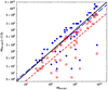 |
Fig. 3. MBH obtained from the SE method from Rakshit et al. (2020) plotted vs. the corresponding values from Wu & Shen (2022). The open squares are the unshifted values and the red short-dashed line indicates the best linear fit. The blue diamonds represent the Rakshit et al. (2020) shifted by a factor 2.5; in this case the blue long-dashed line, which represents the best linear fit, nearly overlaps the one-to-one correlation illustrated by the continuous black line. |
Indeed, when we increase the SE MBH values by a factor of 2.5 and compare them to the X-ray scaling values, the bulk of the AGN becomes consistent (see Fig. 4). We note that very similar figures are obtained (but not shown here) when the MBH values from the catalog of Wu & Shen (2022) without any correction factor are plotted versus the X-ray scaling values. A close look at Fig. 4, where the recalibrated SE MBH values are plotted versus the X-ray based estimates, reveals that (1) the vast majority of the MBH estimates are now in full agreement; (2) the few objects that still have significantly lower SE MBH values compared to the corresponding X-ray ones are based on the C IV line (triangular symbols), are substantially absorbed (see the top panel of the figure, where the color-coded scheme describes the intrinsic absorption), or were flagged in the Rakshit et al. (2020) catalog, which are represented by diamond symbols (there are actually four flagged sources, but two sources perfectly overlap in these plots); (3) the few SE MBH values that are substantially overestimated with respect to the X-ray estimates are sources accreting at super-Eddington rates (see the bottom panel of the same figure, where the color-coded scheme describes the accretion rate in Eddington units).
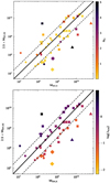 |
Fig. 4. Top panel: SE MBH values multiplied by a factor of 2.5 plotted vs. the X-ray-based values, with color-coded symbols indicating the intrinsic absorption NH in units of 1022 cm−2. Bottom panel: Same as the top panel, with color-coded symbols indicating log(λEdd). The symbols are the same as the ones used in Fig. 2. |
In summary, using the X-HESS sample of Laurenti et al. (2024), we demonstrated that there is a strong positive correlation between the values of MBH obtained with the SE method and those from the X-ray scaling method, indicating that the two methods provide the same relative MBH values. However, our analysis also reveals that the SE-based measurements from the Rakshit et al. (2020) catalog are systematically underestimated by a factor of 2.5. Once the SE-based values of that specific catalog are recalibrated to ensure that they are consistent for moderately accreting AGN, then, in agreement with the current understanding of the limitations of the standard SE method, the discrepancies are limited to extremely highly accreting objects, whose MBH is significantly overestimated by the standard SE method, and to substantially absorbed objects, whose MBH is instead underestimated by the SE method.
3.3. Implications of using different indirect methods
Although the X-ray scaling method and the SE method are broadly consistent with each other, the use of MBH values obtained with the former method specifically from the catalog of Rakshit et al. (2020) (which we now know to systematically underestimate the MBH), including a few sources with mass based on C IV (which our analysis in Section 3.1 confirms to be an unreliable estimator of virial mass) and a few sources that were flagged and therefore deemed unreliable, can have important implications and lead to markedly different conclusions. To illustrate this point, we compared different results obtained using MBH estimates from the X-ray scaling method with some of the corresponding findings derived by Laurenti et al. (2024) with a thorough analysis utilizing the MBH values from the catalog of Rakshit et al. (2020).
Eddington ratio distribution. The first substantial difference is illustrated in Fig. 5, which shows the distributions of the accretion rate values. The distribution obtained with the X-ray method (red color) spreads between log(λEdd) = −2 and 1, whereas by construction the distribution of the X-HESS of Laurenti et al. (2024) based on SE values from Rakshit et al. (2020) is solely restricted to highly accreting objects. The visual difference is quantitatively confirmed by a Kolmogorov–Smirnov test, which yields K = 0.74 and associated probability PK≃10−11.
 |
Fig. 5. Histograms of the log(λEdd) distributions obtained with the X-ray scaling method (red) and the SE method (purple). |
Photon index versus accretion rate. When the photon index Γ is plotted versus log(λEdd), a strong positive correlation is obtained with Spearman coefficient r = 0.54 and relative probability PS = 8×10⁻⁶ and a best fit of Γ=(2.14±0.01)+(0.29±0.01)×log(λEdd) (RMS = 0.26) obtained considering both the X-HESS data (represented by the red diamonds in Fig. 6) and the WISSH data (blue circular symbols). Note that the same strong correlation with a slightly steeper positive slope, Γ=(2.19±0.01)+(0.32±0.01)×log(λEdd), is derived when only the X-HESS sample is used, at odds with the findings of Laurenti et al. (2024), who did not find any significant correlation using the same sample.
 |
Fig. 6. X-ray photon index Γ plotted vs. log(λEdd). The dashed line represents the best fit including both the X-HESS sample (red diamonds) and the WISSH sample (blue circles), Γ=(2.14±0.01)+(0.29±0.01)×log(λEdd). The black squares represent the arithmetic mean obtained by binning the data. |
X-ray bolometric correction versus accretion rate. Markedly different results are also obtained when log(Lbol/LX) (the logarithm of the X-ray bolometric correction factor KX) is plotted versus log(λEdd), as illustrated in the top panel of Fig. 7, where we used the MBH measured with the X-ray method to compute the Eddington ratio. A strong positive correlation is obtained with the X-ray-based values, as confirmed by a Spearman coefficient r = 0.65 and relative probability PS = 1.9×10⁻⁸ and a best fit of KX=(2.26±0.01)+(0.59±0.01)×log(λEdd) (RMS = 0.33). Conversely, no correlation at all is present when SE data are used, as illustrated in the bottom panel of Fig. 7, and confirmed by a statistical analysis: r=−0.04 (PS = 0.75), KX=(1.98±0.01)−(0.03±0.04)×log(λEdd).
 |
Fig. 7. Top panel: Logarithm of the X-ray bolometric correction factor log(Lbol/LX) plotted vs. log(λEdd), where the latter is computed using the X-ray scaling method. The dashed line represents the best fit including both the X-HESS sample (red diamonds) and the WISSH sample (blue circles), KX=(2.26±0.01)+(0.59±0.01)×log(λEdd). Bottom panel: Same plot with log(λEdd) derived using SE measurements. No significant correlation is obtained. |
Soft excess. Finally, we focused on the soft excess. To this end, we extended our spectral analysis to the 0.3−10 keV range (in the observer frame) and added a blackbody component to our baseline model to fit the spectra of sources that show a clear excess (19 in our original sample of 50 AGN), when extrapolating the Comptonized model used to fit the hard X-ray spectrum.
First of all, we verified that different measurements of the strength of the soft excess provide similar results. Indeed, a Spearman analysis (r = 0.89 and relative probability PS = 2.4×10⁻⁷) indicates that log(SX1) = log(Lbb/Lbmc)0.5−2 keV, the quantity similar to that used by Laurenti et al. (2024), is strongly correlated with log(SX3) = log(Lbb,0.5−2 keV/LEdd), the quantity introduced in Gliozzi & Williams (2020) and that will be used again here (for both measurements of the soft excess strength, the uncertainties were calculated with error propagation). This is confirmed by linear regression analysis that yields a best fit of log(SX1) = (1.58±0.04)+(0.63±0.02)×log(SX3) (RMS = 0.32).
Fig. 8 reveals the presence of a strong positive correlation between Γ and log(SX3), described by the best-fit correlation, Γ=(2.75±0.01)+(0.30±0.01)×log(SX3) (RMS = 0.29), and further confirmed by a Spearman coefficient of r = 0.79 and relative probability PS = 4.5×10⁻⁵. Note that similar conclusions at lower significance level are obtained also using log(SX1): Γ=(2.08±0.02)+(0.29±0.03)×log(SX1), r = 0.58 (PS = 9.6×10⁻³). This is again at odds with the results of Laurenti et al. (2024), who inferred the presence of a negative correlation between the photon index and the soft excess strength.
 |
Fig. 8. Photon index plotted vs. the soft excess strength log(SX3) with the best-fit correlation, Γ=(2.75±0.01)+(0.30±0.01)×log(SX3). |
In our statistical analysis we also found a positive correlation between log(SX3) and log(λEdd): log(SX3) = (−1.62±0.05)+(1.07±0.11)×log(λEdd), r = 0.63 (PS = 3.6×10⁻³) (RMS = 0.67), whereas no significant correlation was obtained when the same parameter was plotted versus the hard X-ray luminosity: log(SX3) = (2.67±2.85)−(0.10±0.06)×log(LX), r=−0.12 (PS = 0.63).
4. Discussion
The primary goal of this work is to assess the reliability of the SE method applied to distant AGN. This task is extremely challenging, because direct dynamical methods cannot be applied to distant objects, and other commonly used indirect methods, such as those based on various relationships between MBH and galaxy bulge properties observed in lower-luminosity low-accreting objects in the local universe, may not be suited for highly accreting distant objects. Moreover, since the final goal is to study SMBH-galaxy coevolution over cosmic time, one cannot use the MBH inferred from these correlations.
To assess the reliability of the SE method in distant AGN we used the X-ray scaling method, which has proven to be one of the most reliable indirect methods based on our recent study of a volume-limited, hard-X-ray-selected sample of AGN with MBH dynamically determined (Gliozzi et al. 2024). Since this method is based on a simple Comptonization model (BMC) developed for nearby sources and was essentially used only for local AGN, we first ran a sanity check by applying it to a sample of distant luminous quasars (the X-WISSH sample) with well-defined multiwavelength SEDs completely dominated by the AGN emission (Duras et al. 2020) and for which it is reasonable to assume that accretion occurs at rates close to the Eddington value. This test indicated that the X-ray scaling method yields reasonable MBH values also for distant quasars. Similarly does the SE method based on the Hβ line, whereas the SE method based on the C IV line shows a tendency to systematically overestimate MBH, confirming the conclusions of several studies that questioned the use of high-ionization lines, which are likely to be affected by outflows (e.g., Denney 2012; Denney et al. 2016). Unfortunately, only three sources have MBH measurements obtained with both the X-ray scaling method and the Hβ-based SE method, hampering a quantitative comparison between these two techniques using the X-WISSH sample.
The X-HESS sample presented by Laurenti et al. (2024), which comprises X-ray-bright AGN that are supposedly highly accreting and possess MBH determined with the SE method using primarily the Hβ or Mg II lines, made it possible to carry out a systematic comparison between these two indirect methods. Fig. 2 and the associated analysis reveals a strong linear correlation between the two methods, which indicates that, despite the completely different assumptions, these two methods give consistent results. The same analysis however also shows that the bulk of the moderately accreting objects have systematic differences, with the X-ray-based MBH values being substantially larger than the corresponding SE estimates.
This discrepancy, which is surprising because in the moderately accreting regime the two methods are fully consistent with the values of MBH obtained with the RM technique, can be resolved either by decreasing the X-ray values or by increasing the SE ones by a factor of 2.5. The fact that the average FWHM of lines used to estimate MBH from Rakshit et al. (2020) is systematically smaller than that from Calderone et al. (2017), who use the same data but a different procedure to define and fit the spectral lines, suggests that the MBH values in the Rakshit et al. (2020) catalog are underestimated. Indeed, this hypothesis is confirmed by direct comparison between the MBH values of Rakshit et al. (2020) and the corresponding ones presented by Wu & Shen (2022) in the most recent version of the SDSS catalog for AGN (see Fig. 3). We note that the few MBH values in the X-HESS sample that were obtained with more refined Hβ measurements (Marziani & Sulentic 2014) are fully consistent with the X-ray values, when the sources are not substantially absorbed.
After the two methods are recalibrated by multiplying the SE values by a factor of 2.5 (see Fig. 4), which is on the order of the systematic uncertainty associated with this method (see, e.g., Pancoast et al. 2014), then we obtain a better overall agreement between the two methods. Now the few significant discrepancies are related to (1) sources whose MBH and λEdd values were flagged for poor quality by Rakshit et al. (2020) (namely, source 6 SDSS J172255.24+320307.5, source 14 SDSS J221715.18+002615.0, source 22 SDSS J233317.38−002303.4, and source 34 SDSS J084153.99+194303.1, which are represented by diamonds in Fig. 4); (2) sources whose MBH was computed using the C IV line (source 36 SDSS J090033.50+421547.0 and source 54 SDSS J132654.95−000530.1, which are represented by triangles in Fig. 4); (3) substantially absorbed sources, whose MBH values appear to be underestimated by the SE method in agreement with the findings of Mejía-Restrepo et al. (2022); and (4) sources accreting well above the Eddington ratio, for which the SE method overestimates MBH, as expected from the work of Du et al. (2015, 2018).
While the broad agreement observed between the two methods without applying any recalibration (that is, using the MBH values provided by Rakshit et al. 2020, as done by Laurenti et al. 2024) may suggest that either method could be used interchangeably (after all, a calibration factor of 2.5 is on the order of the typical uncertainty associated with the SE method), our analysis demonstrates this is not the case. Firstly, the distribution of the accretion rates derived from the use of the X-ray-based MBH is substantially broader than the one presented by Laurenti et al. (2024) based on the optically based MBH values from the catalog of Rakshit et al. (2020), suggesting that this sample is not strictly restricted to highly accreting objects (see Fig. 5). Secondly, we find a strong positive correlation when the photon index is plotted versus log(λEdd), in contrast with Laurenti et al. (2024), who found a weak positive correlation only when their data were combined with additional samples spanning a broader range of accretion rates. Our results confirm and strengthen the conclusion that Γ is a faithful indicator of the accretion state of BH systems, as regularly seen in stellar-mass BH systems in their spectral transitions (Remillard & McClintock 2006) and found in several studies based on AGN samples of different redshifts and luminosities (Shemmer et al. 2008; Risaliti et al. 2009; Brightman et al. 2013, 2016; Serafinelli et al. 2017), including long-term spectral variability investigations of individual AGN (Sobolewska & Papadakis 2009).
Additionally, the X-ray bolometric correction KX plotted versus log(λEdd) shows a strong positive correlation only if the Eddington luminosity uses X-ray measurements (see Fig. 7), in agreement with the findings of Lusso et al. (2012) and Duras et al. (2020). The lack of a clear positive correlation when we use the SE values (see the bottom panel of Fig. 7) suggests that the indiscriminate use of MBH values from large catalogs based on automated analysis of spectral data with limited quality may be problematic.
Finally, we find a strong positive correlation between Γ and the strength of the soft excess, in agreement with the results obtained by Bianchi et al. (2009), Boissay et al. (2016), and Gliozzi & Williams (2020). Similarly to the latter study, we also obtain a positive correlation between the strength of the soft excess and the accretion rate, and no correlation at all when the strength of the soft excess is plotted versus the hard X-ray luminosity. All these findings can be naturally explained in the framework where the soft excess is dominated by a warm corona (Done et al. 2012; Różańska et al. 2015; Petrucci et al. 2018). In contrast, Laurenti et al. (2024) inferred the presence of a negative correlation between the photon index and the soft excess strength, which favors the ionized reflection model as the main cause of the soft excess, yet there is no evidence of strong reflection components in any of the spectra of the X-HESS sample.
Before reaching our conclusions, we try to leverage our main results to shed some light on the enigmatic nature of LRDs. Using a sample comprising high-redshift AGN, we find that both the X-ray bolometric correction and the photon index are strongly correlated with the accretion rate measured by λEdd. This confirms that the extreme X-ray weakness of LRGs can be naturally explained by AGN in the highly accreting regime, as proposed by recent theoretical works (Lupi et al. 2024; Pacucci & Narayan 2024; Lambrides et al. 2024; Madau & Haardt 2024): high values of the X-ray bolometric correction factor (KX>103) coupled with a steep photon index (Γ≥2.5) may make moderately luminous very distant AGN virtually undetectable by current X-ray observatories, since the already intrinsically weak X-ray emission is concentrated in the soft part of the spectrum, which falls below the lower energy threshold of current instruments by virtue of the high redshift of these sources. Additionally, our analysis suggests that very highly accreting AGN are likely to have values of MBH substantially overestimated by the standard SE method, lessening some of the constraints on BH growing models and the extreme BH-to-galaxy mass ratios inferred for some of these sources.
5. Conclusions
To conclude, we summarize the main findings of this study.
-
We first verified that the X-ray scaling method yields reasonable estimates of MBH also for distant AGN and quasars.
-
We then used the X-ray scaling method to test the reliability of the SE method applied to highly accreting AGN. The strong correlation between the MBH values obtained with these two different indirect methods is encouraging, given the very different assumptions of the two methods, and suggests that the use of SE MBH values for large population AGN studies is appropriate in most instances.
-
Our comparison of the two methods, however, also indicates the presence of a relevant difference, with SE values taken from the Rakshit et al. (2020) catalog that appear to be consistently smaller than the X-ray-based ones, despite being in a regime of accretion rate and luminosity where the two methods are expected to be fully consistent.
A comparison with other catalogs of SDSS AGN indicates that this discrepancy is related to the specific way that the spectral decomposition and width measurements are performed by Rakshit et al. (2020), which in turn causes the MBH values to be systematically underestimated by a factor of 2.5. Once the SE MBH values are recalibrated, then the only relevant discrepancies are observed for very highly accreting AGN, whose SE-based MBH values are significantly overestimated, and for substantially absorbed AGN, whose SE-based MBH values are instead underestimated.
-
Using the X-ray-based MBH values, we investigated various correlations and confirmed strong positive correlations for the photon index Γ versus the Eddington ratio λEdd and for the X-ray bolometric correction versus λEdd, as well as for Γ versus the soft excess strength, in contrast with the results obtained using SE measurements by Laurenti et al. (2024).
We end with a cautionary note and a speculation on the nature of LRDs. When using SE-based MBH provided in catalogs, one should keep in mind that not all catalogs are equally viable (for example, we have shown that the one from Rakshit et al. (2020) has MBH values systematically underestimated by a factor of 2.5). Additionally, the use of quantities flagged for bad quality and MBH values based on the C IV line should be avoided, since they yield poor estimates of the virial mass.
As for the LRDs, our study confirms that the most extreme super-Eddington sources are very X-ray weak and characterized by steep photon indices, which may explain why LRDs are so difficult to detect by current X-ray observatories. Additionally, our work suggests that the SE MBH values of sources accreting well above the Eddington level appear to be overestimated by about one order of magnitude. We can therefore speculate that LRDs (which are thought to be AGN in an early highly accreting phase) are likely less overmassive than currently thought and this may relax some of the constraints on BH seed models.
Acknowledgments
Based on observations obtained with XMM-Newton, an ESA science mission with instruments and contributions directly funded by ESA Member States and NASA. We thank the referee for the constructive comments and suggestions that have improved the clarity of this paper. MG thanks Misty Bentz for useful discussions and Terrvon L. J. Kelley and Michael Young for their help with the soft excess analysis.
References
- Akylas, A., Papadakis, I., & Georgakakis, A. 2022, A&A, 666, A127 [NASA ADS] [CrossRef] [EDP Sciences] [Google Scholar]
- Arnaud, K. A. 1996, ASP Conf. Ser., 101, 17 [Google Scholar]
- Bañados, E., Venemans, B. P., Mazzucchelli, C., et al. 2018, Nature, 553, 473 [Google Scholar]
- Bentz, M. C., Denney, K. D., Grier, C. J., et al. 2013, ApJ, 767, 149 [Google Scholar]
- Bertemes, C., Wylezalek, D., Rupke, D. S. N., et al. 2025, A&A, 693, A176 [NASA ADS] [CrossRef] [EDP Sciences] [Google Scholar]
- Bianchi, S., Bonilla, N. F., Guainazzi, M., Matt, G., & Ponti, G. 2009, A&A, 501, 915 [NASA ADS] [CrossRef] [EDP Sciences] [Google Scholar]
- Bischetti, M., Piconcelli, E., Vietri, G., et al. 2017, A&A, 598, A122 [NASA ADS] [CrossRef] [EDP Sciences] [Google Scholar]
- Blandford, R. D., & McKee, C. F. 1982, ApJ, 255, 419 [Google Scholar]
- Boissay, R., Ricci, C., & Paltani, S. 2016, A&A, 588, A70 [NASA ADS] [CrossRef] [EDP Sciences] [Google Scholar]
- Brightman, M., Silverman, J. D., Mainieri, V., et al. 2013, MNRAS, 433, 2485 [Google Scholar]
- Brightman, M., Masini, A., Ballantyne, D. R., et al. 2016, ApJ, 826, 93 [NASA ADS] [CrossRef] [Google Scholar]
- Caglar, T., Koss, M. J., Burtscher, L., et al. 2023, ApJ, 956, 60 [NASA ADS] [CrossRef] [Google Scholar]
- Calderone, G., Nicastro, L., Ghisellini, G., et al. 2017, MNRAS, 472, 4051 [Google Scholar]
- Denney, K. D. 2012, ApJ, 759, 44 [NASA ADS] [CrossRef] [Google Scholar]
- Denney, K. D., Horne, K., Shen, Y., et al. 2016, ApJS, 224, 14 [NASA ADS] [CrossRef] [Google Scholar]
- Done, C., & Gierliński, M. 2005, MNRAS, 364, 208 [NASA ADS] [CrossRef] [Google Scholar]
- Done, C., Davis, S. W., Jin, C., Blaes, O., & Ward, M. 2012, MNRAS, 420, 1848 [Google Scholar]
- Du, P., Hu, C., Lu, K. -X., et al. 2015, ApJ, 806, 22 [NASA ADS] [CrossRef] [Google Scholar]
- Du, P., Zhang, Z. -X., Wang, K., et al. 2018, ApJ, 856, 6 [NASA ADS] [CrossRef] [Google Scholar]
- Duras, F., Bongiorno, A., Ricci, F., et al. 2020, A&A, 636, A73 [NASA ADS] [CrossRef] [EDP Sciences] [Google Scholar]
- Elías-Chávez, M., Longinotti, A. L., Krongold, Y., et al. 2024, MNRAS, 532, 1564 [Google Scholar]
- Fan, X., Bañados, E., & Simcoe, R. A. 2023, ARA&A, 61, 373 [NASA ADS] [CrossRef] [Google Scholar]
- Ferrarese, L., & Merritt, D. 2000, ApJ, 539, L9 [Google Scholar]
- Fries, L. B., Trump, J. R., Horne, K., et al. 2024, ApJ, 975, 239 [NASA ADS] [CrossRef] [Google Scholar]
- Gebhardt, K., Bender, R., Bower, G., et al. 2000, ApJ, 539, L13 [Google Scholar]
- Gebhardt, K., Richstone, D., Tremaine, S., et al. 2003, ApJ, 583, 92 [Google Scholar]
- Giacchè, S., Gilli, R., & Titarchuk, L. 2014, A&A, 562, A44 [NASA ADS] [CrossRef] [EDP Sciences] [Google Scholar]
- Gliozzi, M., & Williams, J. K. 2020, MNRAS, 491, 532 [Google Scholar]
- Gliozzi, M., Titarchuk, L., Satyapal, S., Price, D., & Jang, I. 2011, ApJ, 735, 16 [NASA ADS] [CrossRef] [Google Scholar]
- Gliozzi, M., Williams, J. K., & Michel, D. A. 2021, MNRAS, 502, 3329 [NASA ADS] [CrossRef] [Google Scholar]
- Gliozzi, M., Williams, J. K., Akylas, A., et al. 2024, MNRAS, 528, 3417 [NASA ADS] [CrossRef] [Google Scholar]
- GRAVITY Collaboration (Sturm, E., et al.) 2018, Nature, 563, 657 [Google Scholar]
- GRAVITY Collaboration (Amorim, A., et al.) 2021, A&A, 648, A117 [NASA ADS] [CrossRef] [EDP Sciences] [Google Scholar]
- Greene, J. E., Labbe, I., Goulding, A. D., et al. 2024, ApJ, 964, 39 [CrossRef] [Google Scholar]
- Gültekin, K., King, A. L., Cackett, E. M., et al. 2019, ApJ, 871, 80 [Google Scholar]
- Harikane, Y., Zhang, Y., Nakajima, K., et al. 2023, ApJ, 959, 39 [NASA ADS] [CrossRef] [Google Scholar]
- Kaspi, S., Maoz, D., Netzer, H., et al. 2005, ApJ, 629, 61 [Google Scholar]
- Körding, E. G., Jester, S., & Fender, R. 2006, MNRAS, 372, 1366 [CrossRef] [Google Scholar]
- Kormendy, J., & Ho, L. C. 2013, ARA&A, 51, 511 [Google Scholar]
- Labbé, I., van Dokkum, P., Nelson, E., et al. 2023, Nature, 616, 266 [CrossRef] [Google Scholar]
- Lambrides, E., Garofali, K., Larson, R., et al. 2024, ArXiv e-prints [arXiv:2409.13047] [Google Scholar]
- Larson, R. L., Finkelstein, S. L., Kocevski, D. D., et al. 2023, ApJ, 953, L29 [NASA ADS] [CrossRef] [Google Scholar]
- Laurenti, M., Tombesi, F., Vagnetti, F., et al. 2024, A&A, 689, A337 [NASA ADS] [CrossRef] [EDP Sciences] [Google Scholar]
- Lupi, A., Trinca, A., Volonteri, M., Dotti, M., & Mazzucchelli, C. 2024, A&A, 689, A128 [NASA ADS] [CrossRef] [EDP Sciences] [Google Scholar]
- Lusso, E., Comastri, A., Simmons, B. D., et al. 2012, MNRAS, 425, 623 [Google Scholar]
- Macchetto, F., Marconi, A., Axon, D. J., et al. 1997, ApJ, 489, 579 [NASA ADS] [CrossRef] [Google Scholar]
- Madau, P., & Haardt, F. 2024, ApJ, 976, L24 [Google Scholar]
- Magorrian, J., Tremaine, S., Richstone, D., et al. 1998, AJ, 115, 2285 [Google Scholar]
- Maiolino, R., Scholtz, J., Curtis-Lake, E., et al. 2024, A&A, 691, A145 [NASA ADS] [CrossRef] [EDP Sciences] [Google Scholar]
- Martínez-Aldama, M. L., Czerny, B., Kawka, D., et al. 2019, ApJ, 883, 170 [CrossRef] [Google Scholar]
- Martocchia, S., Piconcelli, E., Zappacosta, L., et al. 2017, A&A, 608, A51 [NASA ADS] [CrossRef] [EDP Sciences] [Google Scholar]
- Marziani, P., & Sulentic, J. W. 2014, MNRAS, 442, 1211 [NASA ADS] [CrossRef] [Google Scholar]
- Matthee, J., Naidu, R. P., Brammer, G., et al. 2024, ApJ, 963, 129 [NASA ADS] [CrossRef] [Google Scholar]
- McHardy, I. M., Koerding, E., Knigge, C., Uttley, P., & Fender, R. P. 2006, Nature, 444, 730 [NASA ADS] [CrossRef] [Google Scholar]
- Mejía-Restrepo, J. E., Trakhtenbrot, B., Koss, M. J., et al. 2022, ApJS, 261, 5 [CrossRef] [Google Scholar]
- Merloni, A., Heinz, S., & di Matteo, T. 2003, MNRAS, 345, 1057 [Google Scholar]
- Mortlock, D. J., Warren, S. J., Venemans, B. P., et al. 2011, Nature, 474, 616 [Google Scholar]
- Pacucci, F., & Narayan, R. 2024, ApJ, 976, 96 [NASA ADS] [CrossRef] [Google Scholar]
- Pancoast, A., Brewer, B. J., & Treu, T. 2014, MNRAS, 445, 3055 [Google Scholar]
- Papadakis, I. E. 2004, MNRAS, 348, 207 [NASA ADS] [CrossRef] [Google Scholar]
- Peterson, B. M., Ferrarese, L., Gilbert, K. M., et al. 2004, ApJ, 613, 682 [Google Scholar]
- Petrucci, P. O., Ursini, F., De Rosa, A., et al. 2018, A&A, 611, A59 [NASA ADS] [CrossRef] [EDP Sciences] [Google Scholar]
- Ponti, G., Papadakis, I., Bianchi, S., et al. 2012, A&A, 542, A83 [NASA ADS] [CrossRef] [EDP Sciences] [Google Scholar]
- Rakshit, S., Stalin, C. S., & Kotilainen, J. 2020, ApJS, 249, 17 [Google Scholar]
- Regan, J., & Volonteri, M. 2024, Open J. Astrophys., 7, 72 [NASA ADS] [CrossRef] [Google Scholar]
- Remillard, R. A., & McClintock, J. E. 2006, ARA&A, 44, 49 [Google Scholar]
- Risaliti, G., & Lusso, E. 2015, ApJ, 815, 33 [NASA ADS] [CrossRef] [Google Scholar]
- Risaliti, G., Young, M., & Elvis, M. 2009, ApJ, 700, L6 [NASA ADS] [CrossRef] [Google Scholar]
- Różańska, A., Malzac, J., Belmont, R., Czerny, B., & Petrucci, P. O. 2015, A&A, 580, A77 [NASA ADS] [CrossRef] [EDP Sciences] [Google Scholar]
- Seifina, E., Titarchuk, L., & Ugolkova, L. 2018a, A&A, 619, A21 [NASA ADS] [CrossRef] [EDP Sciences] [Google Scholar]
- Seifina, E., Chekhtman, A., & Titarchuk, L. 2018b, A&A, 613, A48 [NASA ADS] [CrossRef] [EDP Sciences] [Google Scholar]
- Serafinelli, R., Vagnetti, F., & Middei, R. 2017, A&A, 600, A101 [NASA ADS] [CrossRef] [EDP Sciences] [Google Scholar]
- Shaposhnikov, N., & Titarchuk, L. 2009, ApJ, 699, 453 [NASA ADS] [CrossRef] [Google Scholar]
- Shemmer, O., Brandt, W. N., Netzer, H., Maiolino, R., & Kaspi, S. 2008, ApJ, 682, 81 [Google Scholar]
- Shuvo, O. I., Johnson, M. C., Secrest, N. J., et al. 2022, ApJ, 936, 76 [Google Scholar]
- Sobolewska, M. A., & Papadakis, I. E. 2009, MNRAS, 399, 1597 [NASA ADS] [CrossRef] [Google Scholar]
- Steffen, A. T., Strateva, I., Brandt, W. N., et al. 2006, AJ, 131, 2826 [Google Scholar]
- Titarchuk, L., Mastichiadis, A., & Kylafis, N. D. 1997, ApJ, 487, 834 [NASA ADS] [CrossRef] [Google Scholar]
- Venemans, B. P., Findlay, J. R., Sutherland, W. J., et al. 2013, ApJ, 779, 24 [Google Scholar]
- Vietri, G., Piconcelli, E., Bischetti, M., et al. 2018, A&A, 617, A81 [NASA ADS] [CrossRef] [EDP Sciences] [Google Scholar]
- Williams, J. K., Gliozzi, M., Bockwoldt, K. A., & Shuvo, O. I. 2023, MNRAS, 521, 2897 [Google Scholar]
- Woo, J. -H., Wang, S., Rakshit, S., et al. 2024, ApJ, 962, 67 [NASA ADS] [CrossRef] [Google Scholar]
- Wu, Q., & Shen, Y. 2022, ApJS, 263, 42 [NASA ADS] [CrossRef] [Google Scholar]
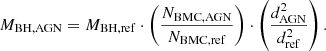
Appendix A: X-ray scaling method in a nutshell
Here we briefly summarize the main characteristics of the X-ray scaling method, since its details have already been described at length in several papers (Shaposhnikov & Titarchuk 2009; Gliozzi et al. 2011, 2021; Williams et al. 2023).
This method lies on two pillars: 1) the luminosity of any BH accreting system is proportional to the MBH, the accretion rate (in Eddington units) ṁ, and the radiative efficiency η and 2) the photon index Γ is a reliable indicator of the accretion state of any BH system. In other words, comparing BH systems with the same Γ ensures that the systems are in the same spectral state and hence have roughly the same values of ṁ and η.
In practice, this method determines the AGN MBH by scaling up the dynamically constrained mass of a stellar mass BH system (the reference source) using two parameters of the BMC model: the spectral index α (where Γ=α+1) and the normalization NBMC. The former ensures that the AGN and reference source are in the same spectral state and the latter computes the actual scaling process:
 (A.1)
(A.1)
Solving for the AGN MBH:
 (A.2)
(A.2)
This process is illustrated by the Γ - NBMC diagram in Fig. A.1, where a generic AGN is compared to the two most reliable reference sources GX 339-4 (whose spectral transition is indicated by the red short-dashed line) and GRO J1655-40 (blue long-dashed line).
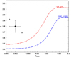 |
Fig. A.1. Γ - NBMC diagram. The black point represents the AGN with its uncertainties (which have been increased for illustration purposes). The red short-dashed line indicates the spectral trend of the reference source GX 339-4. The blue long-dashed line describes the trend of the reference source GRO J1655-40. |
The position of the AGN along the y-axis selects the corresponding spectral state in the reference source, whereas the separation along the x-axis yields the scaling of the MBH. The larger the separation, the smaller the AGN mass; therefore, GRO J1655-40 consistently yields slightly lower values than GX 339-4. For Γ values in the range viable for both reference sources, we computed the MBH values for each reference source and took the average.
The uncertainties on MBH are computed accounting for the uncertainties on the spectral parameters: the distance between point A (defined by the coordinates NBMC−error Γ+error) and the GRO J1655-40 trend defines the minimum MBH, whereas the distance between point B (NBMC+error Γ−error) and the GX 339-4 trend yields the maximum MBH. We note that for sources with relatively flat photon indices (Γ<1.5), only GRO J1655-40 is used, whereas for steeper sources (Γ>1.95) we use only GX 339-4. Finally, for very steep sources (Γ>2.2), we utilize a third reference source, XTE J1550-564, which was not included in Fig. A.1 for the sake of clarity.
Appendix B: Samples used in this paper
WISSH subsample
Auxiliary table for Table B.3
X-HESS subsample
continued.
All Tables
All Figures
|
Fig. 1. Left panel: MBH obtained with the X-ray scaling method plotted vs. the values corresponding to sources accreting at the Eddington level. Middle panel: MBH obtained with the SE method using the C IV line plotted vs. the Eddington values. Right panel: MBH obtained with the SE method using the Hβ line plotted vs. the Eddington values. The symbols are color coded based on redshift. The continuous black line represents the one-to-one correlation and the dashed lines indicate departures by a factor of 3. |
| In the text | |
|
Fig. 2. Left panel: MBH obtained from the SE method using the Hβ line plotted vs. the values derived with the X-ray scaling method, with color-coded symbols indicating the redshift of the sources. Middle panel: Same as the left panel with color-coded symbols illustrating the intrinsic absorption NH in units of 1022 cm−2. Right panel: Same as the left panel with color-coded symbols describing the level of accretion rate, as defined by log(λEdd). Circles indicate MBH based on the Hβ line, squares are values based on the Mg II line, whereas the two triangles indicate the values based on the C IV line; the diamonds represent the sources whose MBH values were flagged as unreliable in Rakshit et al. (2020). |
| In the text | |
|
Fig. 3. MBH obtained from the SE method from Rakshit et al. (2020) plotted vs. the corresponding values from Wu & Shen (2022). The open squares are the unshifted values and the red short-dashed line indicates the best linear fit. The blue diamonds represent the Rakshit et al. (2020) shifted by a factor 2.5; in this case the blue long-dashed line, which represents the best linear fit, nearly overlaps the one-to-one correlation illustrated by the continuous black line. |
| In the text | |
|
Fig. 4. Top panel: SE MBH values multiplied by a factor of 2.5 plotted vs. the X-ray-based values, with color-coded symbols indicating the intrinsic absorption NH in units of 1022 cm−2. Bottom panel: Same as the top panel, with color-coded symbols indicating log(λEdd). The symbols are the same as the ones used in Fig. 2. |
| In the text | |
|
Fig. 5. Histograms of the log(λEdd) distributions obtained with the X-ray scaling method (red) and the SE method (purple). |
| In the text | |
|
Fig. 6. X-ray photon index Γ plotted vs. log(λEdd). The dashed line represents the best fit including both the X-HESS sample (red diamonds) and the WISSH sample (blue circles), Γ=(2.14±0.01)+(0.29±0.01)×log(λEdd). The black squares represent the arithmetic mean obtained by binning the data. |
| In the text | |
|
Fig. 7. Top panel: Logarithm of the X-ray bolometric correction factor log(Lbol/LX) plotted vs. log(λEdd), where the latter is computed using the X-ray scaling method. The dashed line represents the best fit including both the X-HESS sample (red diamonds) and the WISSH sample (blue circles), KX=(2.26±0.01)+(0.59±0.01)×log(λEdd). Bottom panel: Same plot with log(λEdd) derived using SE measurements. No significant correlation is obtained. |
| In the text | |
|
Fig. 8. Photon index plotted vs. the soft excess strength log(SX3) with the best-fit correlation, Γ=(2.75±0.01)+(0.30±0.01)×log(SX3). |
| In the text | |
|
Fig. A.1. Γ - NBMC diagram. The black point represents the AGN with its uncertainties (which have been increased for illustration purposes). The red short-dashed line indicates the spectral trend of the reference source GX 339-4. The blue long-dashed line describes the trend of the reference source GRO J1655-40. |
| In the text | |
Current usage metrics show cumulative count of Article Views (full-text article views including HTML views, PDF and ePub downloads, according to the available data) and Abstracts Views on Vision4Press platform.
Data correspond to usage on the plateform after 2015. The current usage metrics is available 48-96 hours after online publication and is updated daily on week days.
Initial download of the metrics may take a while.