| Issue |
A&A
Volume 675, July 2023
|
|
|---|---|---|
| Article Number | A179 | |
| Number of page(s) | 16 | |
| Section | Stellar structure and evolution | |
| DOI | https://doi.org/10.1051/0004-6361/202243521 | |
| Published online | 18 July 2023 | |
The post-disk (or primordial) spin distribution of M dwarf stars
1
Department of Astrophysics, University of Vienna, Türkenschanzstrasse 17, 1180 Vienna, Austria
e-mail: lukasg90@unet.univie.ac.at
2
Department of Earth Sciences, University of Hawai’i at Mānoa, Honolulu, HI 96822, USA
3
Max-Planck-Institut für Astronomie, Königstuhl 17, 69117 Heidelberg, Germany
Received:
10
March
2022
Accepted:
4
June
2023
Context. The rotation periods of young low-mass stars after disks have dissipated (≲-pagination10 Myr) but before magnetized winds have removed significant angular momentum is an important launch point for gyrochronology and models of stellar rotational evolution; the rotation of these stars also regulates the magnetic activity and the intensity of high-energy emission that affects any close-in planets. A recent analysis of young M dwarf stars suggests a distribution of specific angular momentum (SAM) that is mass-independent, but the physical basis of this observation is unclear.
Aims. We investigate the influence of an accretion disk on the angular momentum (AM) evolution of young M dwarfs, whose parameters govern the AM distribution after the disk phase, and whether this leads to a mass-independent distribution of SAM.
Methods. We used a combination of protostellar spin and implicit hydrodynamic disk evolution models to model the innermost disk (∼0.01 AU), including a self-consistent calculation of the accretion rate onto the star, non-Keplerian disk rotation, and the influence of stellar magnetic torques over the entire disk lifetime. We executed and analyzed over 500 long-term simulations of the combined stellar and disk evolution.
Results. We find that above an initial rate of Ṁcrit ∼ 10−8 M⊙ yr−1, accretion “erases” the initial SAM of M dwarfs during the disk lifetime, and stellar rotation converges to values of SAM that are largely independent of initial conditions. For stellar masses > 0.3 M⊙, we find that observed initial accretion rates Ṁinit are comparable to or exceed Ṁcrit. Furthermore, stellar SAM after the disk phase scales with the stellar magnetic field strength as a power law with an exponent of −1.1. For lower stellar masses, Ṁinit is predicted to be smaller than Ṁcrit and the initial conditions are imprinted in the stellar SAM after the disk phase.
Conclusions. To explain the observed mass-independent distribution of SAM, the stellar magnetic field strength has to range between 20 G and 500 G (700 G and 1500 G) for a 0.1 M⊙ (0.6 M⊙) star. These values match observed large-scale magnetic field measurements of young M dwarfs and the positive relation between stellar mass and magnetic field strength agrees with a theoretically motivated scaling relation. The scaling law between stellar SAM, mass, and the magnetic field strength is consistent for young stars, where these parameters are constrained by observations. Due to the very limited number of available data, we advocate for efforts to obtain more such measurements. Our results provide new constraints on the relation between stellar mass and magnetic field strength and they can be used as initial conditions for future stellar spin models, starting after the disk phase.
Key words: protoplanetary disks / accretion, accretion disks / stars: protostars / stars: rotation / stars: low-mass
© The Authors 2023
 Open Access article, published by EDP Sciences, under the terms of the Creative Commons Attribution License (https://creativecommons.org/licenses/by/4.0), which permits unrestricted use, distribution, and reproduction in any medium, provided the original work is properly cited.
This article is published in open access under the Subscribe to Open model. Subscribe to A&A to support open access publication.
1. Introduction
One of the major challenges in stellar astrophysics is the origin and evolution of stellar angular momentum (AM) and spin. Over the last decade, observations of young clusters have yielded new insight into the evolution of premain sequence (PMS) and young (≲-pagination1 Gyr) main sequence dwarf stars (e.g., Herbst et al. 2002; Irwin et al. 2008; Irwin & Bouvier 2009; Hartman et al. 2009; Meibom et al. 2011; Affer et al. 2013; Gallet & Bouvier 2013). Such coeval groups of stars with established ages and a range of masses provide benchmarks for understanding how that rotational evolution varies with stellar mass and age. The spin evolution of low-mass stars (starting from the Class II phase) can be divided into three phases (Gallet & Bouvier 2013): (1) exchange of angular momentum between a young stellar object (YSO) and its primordial disk; (2) simple contraction and spin-up of the PMS star after the disk has dissipated; and (3) gradual spin-down on the main sequence by loss of AM through a magnetized wind.
Understanding the initial rotation distribution and subsequent evolution of young stars is important to relating stellar rotation to ages (“gyrochronology”; Barnes 2007). Furthermore, rotation drives a magneto dynamo operation in stars with convective envelopes, and magnetic activity is responsible for heating the upper stellar atmosphere, which is the primary source of X-rays and far- and extreme-ultraviolet (XUV) emission from low-mass stars (e.g., Pallavicini et al. 1981; Micela et al. 1985; Pizzolato et al. 2003; Wright et al. 2011; France et al. 2018). XUV irradiation by the host star heats and inflates the upper atmospheres of close-in planets and can lead to evaporation and even complete loss of the atmosphere (e.g., Güdel et al. 1997; Lammer et al. 2003; Cecchi-Pestellini et al. 2009; Lecavelier Des Etangs et al. 2010; Sanz-Forcada et al. 2011; France et al. 2013; Nortmann et al. 2018). XUV-driven loss of water as atomic H can affect the habitability of rocky planets (e.g., Buccino et al. 2006).
These issues come to the fore for studies of M dwarf stars (M⋆ ≈ 0.1 − 0.6 M⊙) as hosts of planets, particularly rocky and potentially habitable planets. M dwarfs are the most common type of star (e.g., Chabrier 2003), and the small size and low mass of M dwarfs favor the detection of planets by the transit and radial velocity methods on close-in orbits. In addition, the lower luminosities of M dwarfs mean that their “habitable zones”, where the equilibrium temperatures of planets would permit surface liquid water, are much closer to the stars (e.g., Zechmeister et al. 2009). However, these stars are intrinsically faint and more difficult to study at the distances of benchmark clusters and as a result, studies and modeling of their rotational evolution and establishment of gyrochronological benchmarks are at an early stage.
Robust measurements of rotation periods for M dwarfs in a few star-forming regions and young clusters have been provided by the precise photometry of the Kepler space telescope, repurposed to observe multiple ecliptic fields in the two-wheel K2 mission (Howell et al. 2014). These groups include the Taurus (1−5 Myr; Rebull et al. 2020), ρ Ophiuchus (3−5 Myr), and Upper Scorpius (∼10 Myr, Rebull et al. 2018) star-forming regions, and the Pleiades (≈125 Myr, Rebull et al. 2016), Hyades (≈650 Myr, Douglas et al. 2019), and Praesepe (≈800, Rebull et al. 2017; Douglas et al. 2017) clusters. Somers et al. (2017) showed that the distributions of specific (per unit mass) angular momentum (SAM) of M dwarfs in Upper Scorpius and the Pleiades were similar, approximately independent of stellar mass, but with a significant scatter. Since by the age of Upper Scorpius circumstellar disks have largely (but not completely) dissipated (Mamajek 2009), the similarity of the two distributions means that angular momentum loss through winds during the first ≤-pagination125 Myr is ≲40%1. It also follows that the origin of the mass-independent SAM distribution lies in the earlier YSO phase and could be a product of the interaction between stars and their disks.
Our study models the YSO phase (≲-pagination10 Myr, e.g., Mamajek 2009) of single M dwarfs to determine if star-disk interactions can explain the observed distribution of SAM and rotation at post-disk times. While the rotational evolution of young, disk-free M dwarfs on the PMS has been previously studied (e.g., Bouvier et al. 2014; Matt et al. 2015), the influence of disks on their rotation is less well explored and most of the work has consisted of long-term spin evolution calculations (e.g., Armitage & Clarke 1996; Matt et al. 2010, 2012; Gallet et al. 2019). During this phase, mass is accreted from the disk onto the star, altering the star’s angular momentum and subsequent rotational evolution. It has been proposed that this exchange leads to the star rotating at the orbital period of the disk inner edge (“disk-locking”, e.g., Ghosh & Lamb 1979; Koenigl 1991). Calculations by Armitage & Clarke (1996) suggest that massive disks coupled to the stellar magnetic field can regulate a star’s spin evolution while low mass disks fail to slow down the star as it contracts and spins up. While Armitage & Clarke (1996) include simplified time-dependent disk evolution in their model, they assume the entire disk couples to the stellar magnetic field lines. However, due to the limited strength of the coupling between the disk and the stellar magnetic field lines the disk may not be able to remove the AM required to balance spin-up due to stellar accretion and stellar contraction and keep the star’s rotation “locked” to the disk (e.g., Matt & Pudritz 2005a; Zanni & Ferreira 2013). Moreover, disk-locking does not explain the existence of very slowly rotating stars (e.g., Matt & Pudritz 2005b).
Other phenomena may be in play during the disk phase: Accretion-powered outflows or winds could also remove angular momentum from the star (APSW, e.g., Matt & Pudritz 2005b, 2008a,b; Matt et al. 2012; Finley & Matt 2018; Gallet et al. 2019). Magnetized disk winds can remove mass and angular momentum from the disk before these are accreted to the star (e.g., Shu et al. 1994; Ferreira et al. 2000; Romanova et al. 2009; Zanni & Ferreira 2013). Magnetospheric ejections, in which the stellar and/or disk magnetic field is loaded with mass from the disk (Zanni & Ferreira 2013), can also transport angular momentum between the star and disk.
Self-consistent modeling of the accretion rate in the disk Ṁdisk and onto the star is important to robustly describe mass and angular momentum exchange. Previous studies fixed the accretion rate to a power law or an exponential decay (e.g., Matt et al. 2010; Gallet et al. 2019) and did not account for feedback between the star and disk. Modeling the disk’s inner edge (≲0.1 au) is numerically challenging because of the short time steps that are required, but this can be achieved with implicit hydrodynamic codes which circumvent the time-step limitations of explicit codes, making long-term simulations feasible (Courant et al. 1928; Ragossnig et al. 2020; Steiner et al. 2021).
Here we combine a model of PMS stellar evolution (Matt et al. 2010) with an implicit hydrodynamic model of disk evolution (TAPIR; Ragossnig et al. 2020; Steiner et al. 2021) that can more realistically and self-consistently calculate disk accretion, the effects of stellar magnetic torques and local pressure gradients, the position of the inner disk boundary, and the effect of the star on the disk. We seek to understand (1) how the parameters describing the star-disk interaction govern the final distribution of SAM when disks have dissipated; and (2) whether the observed, mass-independent distribution of SAM is a natural outcome of our model.
2. Model description
We combine a model of stellar spin evolution (e.g., Matt et al. 2010, 2012; Gallet et al. 2019) with a hydrodynamic description of a protostellar accretion disk. The model used in this study is already described in full detail in Ragossnig et al. (2020) and Steiner et al. (2021) and we refer the reader to these papers for further information. The most important aspects, as well as differences from the version used in Steiner et al. (2021), are highlighted below. Figure 1 schematically illustrates the major features and important parameters of the model.
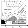 |
Fig. 1. Schematic cartoon of inner disk-star connection. The star (black quarter circle on the left) has a radius of R⋆ and rotates with Ω⋆. Disk material (gray area) flows from the outer disk toward the inner disk radius rin, where it is forced into funnel flows and is accreted onto the star (e.g., Romanova et al. 2004; Bessolaz et al. 2008; Steiner et al. 2021) with an accretion rate of ṀW. The accreted disk material increases the stellar angular momentum by Γacc. Based on the model, a specific fraction of the accreted mass is driven into a stellar wind, which removes mass and angular momentum from the star (Ṁref and ΓW, respectively). The Alfvén radius rA acts as a lever arm for this stellar outflow. We note that this cartoon is not to scale and we can usually assume rA ≫ R⋆. Angular momentum can be transferred toward or away from the star (ΓME), depending on the position of rin with respect to the corotation radius rcor (e.g., Zanni & Ferreira 2013). Finally, magneto-centrifugally driven disk winds remove angular momentum and mass from the disk before it can be accreted on the star (e.g., Königl et al. 2011; Bai & Stone 2013). We note that disk winds are not included in our model. |
2.1. Hydrodynamic disk model
Our simulations model the protoplanetary disk as a time-dependent, viscous accretion disk (e.g., Shakura & Sunyaev 1973; Armitage et al. 2001). Accretion rates are computed self-consistently and are not fixed. We use the one-dimensional implicit TAPIR code (Ragossnig et al. 2020; Steiner et al. 2021), which solves the equations for the surface density Σ, internal energy e and the radial velocity ur as well as the azimuthal velocity uφ (Ragossnig et al. 2020; Steiner et al. 2021). Additionally, the adaptive grid equation introduced by Dorfi & Drury (1987) is solved to ensure sufficient grid resolution and enable moving inner and outer disk boundaries. The accretion disk is assumed to be axisymmetric and in hydrostatic equilibrium in the vertical direction, and thus quasi 2-d. The model allows the velocity to deviate from the Keplerian azimuthal velocity uφ ∼ r−1/2, and effects such as the influence of a stellar magnetic field can be included, being of particular importance in the inner part of the disk (e.g., Romanova et al. 2002; Bessolaz et al. 2008). Models based on the diffusion approximation (e.g., Pringle 1981; Armitage et al. 2001; Zhu et al. 2007, 2010) are not able to include these effects over the whole disk lifetime of ≲-pagination10 Myr. The viscosity model used in this study is based on Shakura & Sunyaev (1973) with the kinematic viscosity ν = αcSHP. Here, α, cS and HP denote the dimensionless viscosity parameter (assumed to range between 0.005 and 0.01, e.g., Zhu et al. 2007; Vorobyov & Basu 2009; Yang et al. 2018), the speed of sound, and the vertical pressure scale height, respectively.
In the inner disk, the stellar magnetic field acts on the partially ionized disk, and the motion of the disk alters the ambient magnetic field. The magnetic field of the star is assumed to be corotating with the star and described as a dipole aligned with the rotation axis and perpendicular to the disk plane. However, the Keplerian motion of the disk tends to wind up locally vertical field lines and generates an azimuthal component of the magnetic field Bφ (e.g., Rappaport et al. 2004; Kluźniak & Rappaport 2007; Steiner et al. 2021). The motion of ionized disk gas with respect to the local magnetic field induces a torque in the azimuthal direction and thus leads to an acceleration in the radial direction (e.g., Romanova et al. 2002). The resulting drop in disk surface density toward the star (e.g., Bessolaz et al. 2008; Steiner et al. 2021) creates a pressure gradient. The torque, induced by the stellar magnetic field, changes sign at the corotation radius
with G being the gravitational constant, M⋆ the stellar mass and P⋆ the stellar rotational period. Interior to rcor, the disk gas is decelerated in the azimuthal and accelerated in the radial direction toward the star. Exterior to rcor, the disk material is accelerated in the azimuthal direction, pushing it away from the star. Toward the innermost part of the disk, the magnetic pressure ( ) overwhelms the gas pressure as well as the ram pressure of the disk material moving toward the star. At a so-called truncation radius rtrunc, the disk material is forced along magnetic field lines and is “funneled” toward the star (e.g., Romanova et al. 2002; Romanova & Kurosawa 2014). We choose rtrunc to be the inner radius of the accretion disk rin; this radius is calculated by equating the stellar magnetic pressure to the disk’s ram pressure or gas pressure at the inner boundary, whichever is higher (see Steiner et al. 2021). Similar to Romanova et al. (2002) and Steiner et al. (2021), the inner boundary is treated as a “free” Neumann boundary (i.e., ∂rΣ = 0). At the outer boundary, the azimuthal velocity uφ equals the Keplerian velocity, the radial velocity ur is set to zero, and the surface density Σ as well as the internal energy e are again treated with Neumann boundary conditions. The outer disk radius is set to the position where the disk surface density has declined to Σout = 1 g cm−2 (similar to Vorobyov et al. 2020).
2.2. Stellar spin model
The stellar spin evolution model used in this study is based on the work of Matt et al. (2010) and Gallet et al. (2019). The simulations are started from a stellar age of t0 = 1 Myr (similar to Gallet et al. 2019), an age corresponding approximately to the beginning of the Class II YSO phase when the only significant accretion is through a disk. The star is considered to be fully convective and to rotate as a solid body. The stellar angular momentum can be written as J⋆ = I⋆Ω⋆, with a moment of inertia  including the stellar radius R⋆ as well as the dimensionless radius of gyration k and the stellar angular velocity Ω⋆. We assume k2 = 0.2 to be constant in time, which is a reasonable assumption over the first 10 Myr (e.g., Armitage & Clarke 1996; Matt et al. 2010, 2012). J⋆ is altered by external torques Γext of which, following the formulation in Gallet et al. (2019), we model three torque components:
First, the accretion torque, Γacc: The accretion of disk material adds mass and angular momentum to the star. Γacc is the product of the accretion rate onto the star and the specific angular momentum of the disk at the inner disk boundary (e.g., Gallet et al. 2019). This torque contribution is positive, which means that the star spins up due to the accretion of disk material.
Second, accretion-powered stellar winds (APSW), ΓW: In the picture of a magnetized stellar outflow, the ejected material is magneto-centrifugally accelerated along stellar magnetic field lines. As the wind propagates outward, it removes angular momentum from the star and results in stellar spin-down. In this study, the driving force of this wind is considered to be accretion (accretion-powered stellar wind, APSW, e.g., Matt & Pudritz 2005a; Gallet et al. 2019) and the mass-loss rate scales as ṀW = WṀ⋆, with the APSW efficiency parameter, W. The Alfvén radius rA acts as a lever arm for this stellar outflow and controls how much angular momentum is carried away (e.g., Gallet et al. 2019; Pantolmos et al. 2020; Ireland et al. 2021). We note that the order of W as well as the driving forces of the APSW are still under debate (see Sect. 4.3 or, e.g., Gallet et al. 2019).
Third, Magnetospheric ejections (ME), ΓME: Angular momentum can be transferred between the star and the disk by magnetospheric ejections if the stellar magnetic field is strong enough to couple to the disk material (e.g., Zanni & Ferreira 2013; Gallet & Bouvier 2013). Starting from vertical stellar magnetic field lines that corotate with the star, differential rotation between the star and the disk generates a toroidal field component. The toroidal field results in a pressure component in the vertical direction that induces a periodic inflation and reconnection process of the magnetic field lines (Zanni & Ferreira 2013). The angular momentum transferred by this process, ΓME, depends on the twist of the field lines, the stellar magnetic field strength, and the radial disk region that couples to the magnetic field lines (e.g., Zanni & Ferreira 2013; Gallet et al. 2019). The sign of ΓME results from the relation between the inner disk boundary, rtrunc, and the corotation radius, rcor. If the ratio between the truncation radius and the corotation radius is smaller than a given value KME, rtrunc/rcor < KME, the MEs spin up the star. For larger truncation radii, rtrunc/rcor ≥ KME, the MEs spin down the star. The dimensionless parameter, KME, results from a best-fit value based on multidimensional models of the star-disk interaction (e.g., Gallet et al. 2019; Pantolmos et al. 2020). The value of KME varies between different studies and ranges between 0.60 (Pantolmos et al. 2020) and 0.79 (Gallet et al. 2019). In this study, we choose the latter.
Internal redistribution of angular momentum resulting from the development of a radiative core (as described in Gallet et al. 2019) is neglected because very low-mass stars will remain fully convective during the disk lifetime and rotate as solid bodies. The evolution of the stellar rotation is governed by changes in AM and changes in the moment of inertia due to mass accretion and PMS contraction (e.g., Matt et al. 2010; Gallet et al. 2019). The rate of stellar mass change is calculated by the hydrodynamic disk model as the disk accretion rate at the inner boundary and we describe the stellar radius evolution by Kelvin-Helmholtz contraction with an index 3/2 polytrope (e.g., Collier Cameron & Campbell 1993; Matt et al. 2010, 2012), resulting in
with the stellar effective temperature Teff and the Stefan-Boltzmann constant σ. The deviation of Eq. (2) from radii predicted by the PMS model of Baraffe et al. (2015) is only ∼1% over the first 10 Myr.
2.3. Parameter range
We define a parameter range for our simulation that agrees reasonably with observations and theoretical estimates of stellar and disk parameters.
2.3.1. Stellar rotation period of T Tauri stars
Over the last two decades, the rotation periods of a large number of young (≲-pagination10 Myr) stars have been measured (e.g., Herbst et al. 2002; Rebull et al. 2006, 2010, 2015, 2020; Cody & Hillenbrand 2010; Venuti et al. 2017; Serna et al. 2021, as well as other publications by the YSOVAR consortium). In Fig. 2, the distributions of rotation periods of five of these studies are shown. The majority of periods are located between ∼1 and 10 days. The distribution decreases strongly toward ∼20 days and there are very few stars with rotation periods > 20 days. This distribution of values, however, has to be treated with caution. Studies based on TESS observations (e.g., Rebull et al. 2015; Serna et al. 2021) are biased against periods longer than TESS’ lunar-synchronous orbit of 13.7 days (e.g., Howard et al. 2021; Claytor et al. 2022) and longer undetected periods are possible2. Furthermore, ground-based studies are subjected to the known effect of decreased sensitivity to longer periodic signals that are near the threshold of detection (only a few periods can be coadded for detection). We adopt a conservative range of 1−10 days, recognizing that there are some stars with initial rotation periods outside this range.
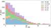 |
Fig. 2. Distribution of stellar rotation periods in young clusters: ONC (R+06, Rebull et al. 2006), σ Ori (C+H10, Cody & Hillenbrand 2010), NGC 2264 (V+17, Venuti et al. 2017), Taurus (R+20, Rebull et al. 2020) and the Orion star forming region (S+21, Serna et al. 2021). |
2.3.2. Stellar magnetic dipole field strength
The dipole magnetic field strength is an important parameter for the spin model used in this study. Obtaining reliable estimates of B⋆, however, is challenging due to the limited number of observations and complex physical processes that generate the magnetic field (e.g., Kochukhov 2021). There are different techniques for measuring magnetic fields (e.g., the review of Kochukhov 2021, and references therein). In the most common method, the broadening of magnetically sensitive lines due to the Zeeman effect is measured and the strength of the magnetic field is described in terms of the Stokes I parameter. We refer to this B-field measurement as BI. BI is a measure of the total intensity of the surface magnetic field and it is not possible to differentiate between small and large-scale components. A more detailed technique, Zeeman-Doppler imaging (ZDI), resolves the distribution of line broadening on the stellar surface and obtains the Stokes V parameter (e.g., Johnstone et al. 2014). A large-scale magnetic field dipole component (which we refer to as BV) can be calculated from this. We note that there is the possibility that BV can underestimate the strength of the magnetic field as it can be partially canceled out by higher-order components (see the case of AU Mic, Kochukhov & Reiners 2020). If, in addition to the Stokes I and V parameters, the Stokes Q and U parameters are available, the overall structure of the stellar magnetic field and a more precise value for the large-scale field can be calculated (e.g., Kochukhov & Reiners 2020). We refer to this large-scale field measurement as BQU. Unfortunately, this requires observationally expensive high-resolution spectropolarimetry, and these have been performed on very few stars (Kochukhov & Reiners 2020). The large-scale dipole field component (inferred indirectly based on Stokes V or Stokes Q and U parameters) usually dominates the magnetic star-disk interaction and governs the loss of AM due to the APSW (e.g., Finley & Matt 2018); it is this component that is parameterized by the surface field parameter B⋆ in this study.
Aggravatingly, the stellar magnetic field evolves with time (e.g., Folsom et al. 2016). Young, fully convective stars have a strong, axisymmetric, and predominantly dipolar field. As the stars evolve and develop a radiative core (stars with masses ≲0.3 M⊙ stay fully convective during their entire lifetime), the field strength decreases, and the field complexity increases, reducing the dipole component (e.g., Folsom et al. 2016). Based on the data for 8 T Tauri stars, the large-scale field comprises up to blsf ≈ 42% of the total field intensity (e.g., Lavail et al. 2019) ranging from ∼0.1 kG up to ∼2 kG in their sample. For M dwarfs, the total field strength can range up to ∼8 kG (Reiners et al. 2022). Additionally, we want to highlight the case of AU Mic (Kochukhov & Reiners 2020). AU Mic is a 22 Myr-old, partially radiative M dwarf with a total field intensity of 2.3 kG and a dipole component of 2.0 kG, corresponding to blsf ≈ 87% of the total intensity. As AU Mic has already developed a radiative core, the previously mentioned evolutionary trends (Folsom et al. 2016) allow the possibility of an even larger proportion of the large-scale field component blsf at younger ages.
Based on the aforementioned limitations and the small number of available observations, we note that reliable estimates of magnetic field strengths are difficult to obtain. The range of dipole field strengths from 0.1 kG to 2.0 kG used in this study covers most of the dipole field strengths inferred from observations. However, we do not exclude the possibility of higher and lower dipole field strengths.
2.3.3. Initial disk accretion rates
As shown in previous studies, the spin evolution of young stars depends on the initial accretion rate (e.g., Gallet et al. 2019). Therefore, it is important to define realistic initial accretion rates over the M dwarf mass range at the starting point of our simulations, which is the beginning of the Class II phase. Age estimates of young Class II objects start at ≳1 Myr but show a significant spread of ∼1 Myr, which complicates reliable estimates for the accretion rate at the beginning of the Class II phase (e.g., Manara et al. 2012; Fiorellino et al. 2021; Testi et al. 2022). As a consequence, we motivate the choice of our initial accretion rates in this study not based on age estimates, but on the comparison of accretion rates of different evolutionary stages of the star-disk system.
In Fig. 3, observed accretion rates of Class I (assumed ages < 1 Myr, e.g., Fiorellino et al. 2022), Class II, and “flat spectrum” objects are summarized (see caption for references). Flat spectrum (or transition) objects are characterized by a flat spectral energy distribution (SED, e.g., Tobin et al. 2020), indicating the transition between Class I and Class II. Based on the observed sources, accretion rates of flat spectrum sources (blue squares) are located between Class I (gray lines) and Class II (red lines) objects. Thus, we choose the flat spectrum sources as initial values for our simulations. The solid blue line represents the fit and is taken as a reference value (Ṁref) for the initial accretion rates in the further course of this study and scales as
 |
Fig. 3. Observed accretion rates of Class I (gray), Class II (red), and flat spectrum (blue) sources. The gray dash-dotted line is taken from Fiorellino et al. (2021) and the gray dotted line from Caratti o Garatti et al. (2012). The gray-shaded area is limited by the two lines. The red dashed, dotted, and dash-dotted lines are taken from Manara et al. (2012), Fiorellino et al. (2021), and Testi et al. (2022), respectively. The red-shaded area has a minimum but constant logarithmic height so that all red lines are comprised. The thick gray and red lines indicate the mean values of the Class I and Class II objects. The blue squares represent accretion rates of flat spectrum sources (summarized in Table B.1). The blue line is the best fit for the flat spectrum objects and the dashed line is five times less than that, just above the Class II regime. |
Due to large uncertainties in the observed accretion rate (e.g., Caratti o Garatti et al. 2012), we also consider smaller (by a factor of 5) initial accretion rates Ṁlow; these values are located at the upper edge of the typical values for Class II objects for all values of M⋆ (dashed blue line in Fig. 3).
3. Results
We describe two sets of results: first, the influence of an accretion disk on stellar SAM and how the spin evolution of M dwarfs varies with different initial stellar and disk parameters (Sect. 3.1); and second, how the post-disk specific angular momentum (SAM) of M dwarfs depends on stellar and disk parameters (Sect. 3.2). In all simulations, the disk is considered to be dissipated and simulations are stopped when the accretion rate falls below 10−13 M⊙ yr−1. This is the minimum disk accretion rate that can be detected on M dwarfs with current observational methods (Sicilia-Aguilar et al. 2016). At this accretion rate, the residual disk typically has a mass of ∼10−6 M⊙ and ceases to influence the stellar rotation.
Our simulations yield both disk accretion rates and lifetimes that are consistent with observations and empirical descriptions of disk accretion based on observations. Figure 4 compares disk accretion rate vs. time from our simulations to an empirical power-law relation Ṁ ∝ t−χ (Eq. (3) in Gallet et al. 2019), where χ is a fitting parameter. Two cases are shown: The blue (red) line Ṁex(1)(t) (Ṁex(2)(t)) represents our simulations with a star with M⋆ = 0.3 (0.1) M⊙ and a disk with a viscous parameter α = 0.005 (0.010), respectively. The stellar magnetic field strength is the same (B⋆ = 1 kG) in both cases. The power-law exponent takes values of χ = 1.2 (solid black line, Gallet et al. 2019) and χ = 1.5 (dashed black line, Vasconcelos & Bouvier 2017). For disk lifetimes of 7.2 and 3.5 Myr, our simulations are in reasonable agreement with the empirical power law. We note that the lifetimes among our simulations range between ∼2 and 11 Myr. This range is comparable to disk lifetimes, inferred from observations (e.g., Richert et al. 2018; Pfalzner et al. 2022, and references therein). Accretion rates that are initially ≳10−8 M⊙ yr−1 are also predicted to fall below 10−9 M⊙ yr−1 within a few Myr (Fig. 4), consistent with the range of accretion rates observed in clusters at such ages (Manara et al. 2022).
 |
Fig. 4. Model disk accretion rates vs. time for two cases: The Ṁex(1)(t) (blue line) and Ṁex(2)(t) (red line) cases are simulations of stars with M⋆ = 0.3 (0.1) M⊙ and a disk with a viscosity parameter α = 0.005 (0.010), respectively. The stellar magnetic field strength is the same (B⋆ = 1.0 kG) in both cases. We compare these to empirical relations based on the power-law relation Ṁ ∝ t−χ of Gallet et al. (2019) with disk lifetimes of 3.5 and 7.2 Myr and exponents χ = 1.2 (solid black line) and χ = 1.5 (dashed black line) (Vasconcelos & Bouvier 2017; Gallet et al. 2019). |
3.1. The influence of a disk on stellar AM
To study the influence of an accretion disk on the central star, we consider different initial values for the stellar and disk AM and compare the final stellar AM to its initial value once the disk has dissipated. For a given initial stellar radius and mass, the stellar AM in our model can be changed by varying the initial rotational period Pinit. Since the disk is in quasi-Keplerian rotation, its AM can be adjusted by changing the disk mass, which we do by varying its initial accretion rate Ṁinit for a fixed α (Ṁ ∝ αΣ for a viscous accretion disk; see Armitage 2013).
To illustrate the varying effect of disks with different initial accretion rates on the final stellar AM and rotation period, we consider, as a fiducial case, a 0.3 M⊙ star with a photospheric magnetic field of B⋆ = 0.5 kG. The disk’s viscous α parameter is set to 1 × 10⁻² and we set the efficiency of a stellar wind to W = 2%. Pinit is varied from 1 to 10 days and we vary Ṁinit from 10−12 to 3 × 10⁻⁸ M⊙ yr−1 (see Sect. 2.3). Figure 5 plots the final stellar rotation period at disk dissipation as a function of Pinit and Ṁinit. For a more intuitive interpretation of this plot, we show the initial and final rotation periods instead of the SAM values. The same conclusions can be drawn for SAM because the duration of these simulations is short compared to the Kelvin-Helmholtz contraction time ( ) of the star and thus the stellar moment of inertia does not change significantly.
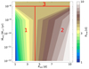 |
Fig. 5. Final stellar rotation period Pfinal for different initial periods Pinit and disk accretion rates Ṁinit. The stellar and disk parameters are: B⋆ = 1000 G, M⋆ = 0.3 M⊙, W = 2% and α = 0.01. We can divide the parameter space into three different regions, separated by red lines (see text). |
In our stellar spin model (see Sect. 2.2), Pfinal in Fig. 5 is influenced by accretion, the magnetic star-disk connection, and the APSW. These quantities are calculated self-consistently and depend on time and on stellar and disk parameters (see Steiner et al. 2021). Contrary to the effects of accretion and the APSW, which (in our model) always spin up and spin down the star, respectively, MEs can result in a spin-up or spin-down torque that acts on the star. As described in Sect. 2.2 and, for example, in Gallet et al. (2019), the position between the truncation radius and the corotation radius determines the sign of this torque contribution. MEs spin up the star if the truncation radius is located well within the corotation radius. In case the truncation radius moves outward and toward the corotation radius, MEs can spin down the star (e.g., Gallet et al. 2019).
For a given truncation radius (rtrunc < rcor), the corotation radius of a star that spins up moves inward, and the distance between rtrunc and rcor decreases. Thus, the spin-up torque of the MEs is reduced or even turned into a spin-down torque in the case of a faster-rotating star. Following the same logic, the MEs tend to increase the spin-up torque onto the star, if the star spins down. For a given stellar rotation and corotation radius, an increased accretion rate can also alter the effects of the MEs. A high accretion rate pushes the truncation radius inward and the distance between rtrunc and rcor increases. Thus, the MEs tend to spin up the star during phases of high accretion rates. Analogously, the distance between the truncation and corotation radius decreases during phases of low accretion rates, and the MEs spin down the star.
Furthermore, the strength and sign of the MEs depend on the magnetic field strength. A strong stellar magnetic field strength results in larger truncation radii. As a consequence, the MEs tend to show a spin-down tendency for strong stellar magnetic field strength. For weak stellar magnetic fields, on the other hand, the distance between the truncation and corotation radius increases, and the MEs show a spin-up tendency. Furthermore, the magnitude of the torque due to MEs is proportional to  (e.g., Gallet et al. 2019) and the overall effect of MEs on the stellar spin evolution increases in case of strong magnetic field strengths.
We note that the sign and magnitude of the torque due to MEs, ΓME, are strongly coupled to different (in turn coupled) parameters such as the accretion rate, stellar rotation period, and magnetic field strength. We show the evolution of ΓME in Fig. A.1 for different configurations. As expected, the MEs result in a spin-up torque for high accretion rates during the beginning of our simulations, weak magnetic field strengths, or slow rotation periods. For fast-rotating stars and strong magnetic field strengths during phases of low accretion rates (especially toward the end of the disk lifetime), MEs spin down the star. Compared to the spin-down torque of APSW (see Fig. A.1), the effect of MEs is comparable for very fast-rotating stars. MEs are even the dominant source of stellar AM loss during the last ≳1 Myr of the disk lifetime.
We can divide the parameter space in Fig. 5 into three regions (demarcated by red lines). In Region 1 (2), the star-disk interaction causes the stellar period to increase (decrease), respectively. The influence of the disk, however, is not strong enough to erase the imprint of the initial stellar spin values. A rapidly rotating star remains rapidly rotating compared to a slow rotator and the dispersion in the final states is comparable to the spread of initial values. In this regime, at the bottom of Fig. 5, the contours are more vertical. In Region 3, the accretion disk is the dominant factor that controls the stellar spin evolution during the disk phase, the initial conditions are forgotten, and Pfinal converges toward a narrower range of values, nearly independent of Pinit. This is the regime at the top of Fig. 5 where the contours are nearly horizontal. The star’s initial rotation state is “erased” by the interaction with the disk. This phenomenon has been seen in previous studies (e.g., Armitage & Clarke 1996; Matt et al. 2012) but the dependence of this behavior on star and disk parameters has not been investigated.
To investigate how this behavior depends on stellar and disk properties other than accretion rate, we vary these parameters: the strength of the star’s magnetic dipole field at its surface B⋆ ∈ [0.5, 1 kG] (see Sect. 2.3), the initial stellar mass M⋆ ∈ [0.3, 0.6 M⊙], and the disk viscous parameter α ∈ [0.005, 0.01]. The resulting effect of the accretion disk on the stellar spin evolution is visualized by comparing the ratios between maximum and minimum values of the stellar rotational period and the specific angular momentum after the disk has been dispersed relative to the ratios of the initial values. A parameter C is introduced to quantify the change of these ratios by the following relations
and
The left-hand sides of Eqs. (4) and (5) denote the stellar rotational periods and specific angular momentum values after the disk has been dissolved (final values) and the right-hand sides the respective initial values. C can be understood as the slope of the contours in a log-log plot (Fig. 5). A value of C close to 1 corresponds to a weak influence of the accretion disk. A strong influence on the stellar spin evolution on the other hand is indicated by C ≪ 1. In this case, the initial rotational values are “forgotten” and the star’s final state is independent of the initial rotation. We consider C = 0.01 (corresponding to a final difference of ≈2%) sufficiently low for final conditions to be convergent and define the initial accretion rate at which this condition is reached as a critical accretion rate Ṁcrit.
We quantify the effect of variation of the parameters disk viscosity (α), stellar wind (W), stellar magnetic field (B⋆), and stellar mass (M⋆) on Ṁcrit in Fig. 6. These parameters, α in panel a, W in panel b, B⋆ in panel c, and M⋆ in panel d, determine the spin-down behavior. Therefore, for each set of parameters, we can identify a value of Ṁcrit that is ∼10−8 M⊙ yr−1. Above this value, the stellar rotational period, as well as the SAM, do not depend on their initial values.
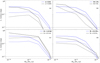 |
Fig. 6. C-parameter (the gradient of the contours in Fig. 5) with respect to initial disk accretion rates Ṁinit. The solid lines represent CP and the dashed lines Cj values, respectively. Each subplot shows variations in (a) viscous α parameter: 0.01 (blue lines) and 0.005 (black lines). The stellar mass is 0.3 M⊙ with a magnetic dipole field strength of B⋆ = 1 kG. (b) W values: 2% (blue lines) and 5% (black lines). The stellar mass is 0.3 M⊙ with a magnetic dipole field strength of B⋆ = 1 kG and a viscosity parameter of α = 0.01. (c) B⋆ values: 1.0 kG (blue lines) and 0.5 kG (black lines). The stellar mass is 0.3 M⊙ with a viscosity parameter of α = 0.01. (d) M⋆ values: 0.3 M⊙ (blue lines) and 0.6 M⊙ (black lines). The viscosity parameter is α = 0.01. The threshold of C = 0.01 for the star to be in the “locked”-state is indicated by the horizontal dotted line. For better visualization, the highlighted parameters show the reference value in the other subplots. |
3.2. Relations for the post-disk specific angular momentum
We examine the dependencies of the SAM after the disk phase on stellar and disk parameters. We compare these to the distribution of SAM among M dwarfs in the Upper Scorpius star-forming region reported by Somers et al. (2017). This sample is especially suitable for studying the AM distribution after the disk phase because the cluster has an age of ∼10 Myr (Feiden 2016) and most accretion disks dissipate by that time (Mamajek 2009); also there’s been no significant loss of AM from a thermal stellar wind up to this age. Somers et al. (2017) provided a mean and standard deviation for SAM in mass bins of 0.10 − 0.25 M⊙, 0.25 − 0.40 M⊙ and 0.40 − 0.60 M⊙, respectively.
3.2.1. Influence of stellar parameters on the post-disk SAM
We perform a set of simulations to examine the effect of varying stellar mass and magnetic field on the final (post-disk) SAM of the star, jfinal. The initial stellar mass is set to 0.1, 0.3, 0.5 M⊙, reflecting the three mass bins of Somers et al. (2017). We note that during the simulations the stellar mass is increased by ≲5% due to the accretion of disk material. Three different initial stellar rotation periods are assumed: 1, 3, and 10 days. We adopt initial accretion rates that correspond to an evolutionary stage just preceding the classical T Tau stage, namely those of flat-spectrum transitional Class I to Class II sources (Tobin et al. 2020); these empirically determined accretion rates are mass dependent (see Eq. (3)). In addition, the magnetic dipole field strength is set to values of 0.1, 0.2, 0.4, 0.7, 1.0, and 2.0 kG. The viscous parameter is set to α = 0.01. The SAM after the disk phase jfinal for each possible combination is shown in Fig. 7. The colored circles, crosses, and squares represent initial rotation periods of 1, 3, and 10 days, respectively, and the solid, dash-dotted, and dashed lines show the respective fits. Mean and standard deviation values for the observed SAM taken from Somers et al. (2017) for each mass bin are represented by gray solid and dashed lines, respectively.
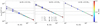 |
Fig. 7. The SAM after the disk phase jfinal for different stellar magnetic field values and stellar masses of 0.1 M⊙ (panel a), 0.3 M⊙ (panel b), and 0.5 M⊙ (panel c). The colored circles, crosses, and squares represent initial rotation periods of 1, 3, and 10 days, respectively, and the solid, dash-dotted, and dashed lines show the respective fits. Mean and standard deviation values for the SAM taken from Somers et al. (2017) are represented by gray solid and dashed lines, respectively. |
For stellar masses, ≳0.3 M⊙ the initial accretion rate is ≳ Ṁcrit (see Eq. (3)) and rotation period at the end of the disk phase is largely independent of the initial period (see panel c). For stellar masses, < 0.3 M⊙, the initial accretion rates are below the critical value and the initial rotation period influences the final value for B⋆ < 1 kG (see panel a). The ensemble of outcomes is well represented by power laws of the form  . The magnetic field strengths of the intersection between the fitted data and the mean values from Somers et al. (2017) (
 ) and the exponents b are summarized in Table 1.
Values of  , b, and jref for models with Ṁref.
3.2.2. Influence of disk parameters on jfinal
To study how the jfinal relations derived in Sect. 3.2.1 depend on the assumed values for disk parameters, we vary the initial accretion rate, the viscosity value α, as well as the APSW efficiency W and compare the results to the standard cases described in the previous subsection. In Fig. 8, the results are shown and in Table 2, the magnetic field strengths of the intersection between the fitted data and the mean values from Somers et al. (2017) ( ) and the exponents b are reported. In the following cases, the initial stellar mass is set to 0.3 M⊙. For comparison, the yellow lines show the fits from Fig. 7 for a stellar mass of 0.3 M⊙.
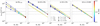 |
Fig. 8. The SAM after the disk phase jfinal as a function of stellar magnetic field values (x-axis and colors) and for different initial rotation periods (different sets of point styles and curves). Each panel shows the variation of one parameter with respect to the reference case in Fig. 7. In panel a, Ṁlow is used as the initial accretion rate. In panels b and c, the APSW efficiency is set to 0% and 5%, respectively. In panel d, the viscous α parameter is set to 0.005. In all cases, the stellar mass is 0.3 M⊙. The symbols and lines are identical to Fig. 7. For comparison, the yellow lines show the fits from Fig. 7 for a stellar mass of 0.3 M⊙. |
Values of  and b for models with Ṁlow, W = 5%, and α = 0.005.
We reduce the initial accretion rate by a factor of 5 compared to the values generated by Eq. (3). At the lower initial accretion rates Ṁlow (panel a), the star-disk interaction is weaker than in the reference case, and jfinal is more strongly influenced by the initial conditions. As a result, the difference between  and b for fast and slow initial rotation periods is larger. More intuitively, if the predicted values of jfinal are to agree with the observations, a larger variation in B⋆ and the exponent b is needed to compensate for variations in the initial rotation period.
The amount of AM that is removed by the APSW is controlled by the efficiency parameter W. As a consequence, the values for jfinal are shifted in the vertical direction toward higher (lower) values for smaller (larger) values of W, respectively. The values for the magnetic field strengths of the intersection between the fitted data and the mean values from Somers et al. (2017),  , are nearly equally increased (reduced) by 530 G (137 G) in case of W = 0% (W = 5%) (see panels b and c in Fig. 8 and Table 2). At a given accretion rate, a lower value of α increases the disk mass and lifetime, allowing star-disk interaction to influence the stellar AM over a longer time period and reducing the critical accretion rate (see panel a in Fig. 6). The values in
  and b for different Pinit values converge and the initial conditions are now (nearly) completely forgotten (panel d in Fig. 8).
The stellar SAM after the disk phase can be described by a power law such as
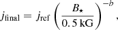
with the proportionality factor jref, depending on the stellar mass and, if Ṁinit < Ṁcrit, also on the initial stellar rotation period Pinit. The values for jref for our reference case are summarized in Table 1.
4. Discussion
We now wish to discuss the consistency of our results with observations, resulting implications, limitations, and uncertainties due to initial conditions and the adopted ranges of our principal parameters.
4.1. Comparison of  with inferred dipole field strengths
We compare the values of  that are required to explain the observed SAM to the dipole field strengths observed or inferred on young, low-mass stars. In Fig. 9, dipole magnetic field strengths are shown with respect to the stellar mass. Solid black circles show dipole field strengths inferred by the Stokes V parameter (BV), open circles indicate an estimate based on the total field intensity (BI), and a dipole field strength fraction of blsf = 22% (Lavail et al. 2019), and the black diamond indicates the dipole field strength of AU Mic, the only young star in our sample with direct measurement of BQU. The data is taken from Yang & Johns-Krull (2011), Johnstone et al. (2014), and Table C.1. It is important to note that, for this comparison, young accreting and nonaccreting stars are combined to increase the number of available data points. To minimize the effect of an evolving magnetic field, the age of the nonaccreting stars is restricted to the disk dispersal age (see Table C.1).
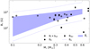 |
Fig. 9. Observed dipole field strengths of young stars with respect to stellar mass. Solid black circles show dipole field strengths inferred by the Stokes V parameter (BV), open circles indicate an estimate based on the total field intensity (BI) and a dipole field strength fraction of blsf = 22% (Lavail et al. 2019), and the black diamond indicates the dipole field strength of AU Mic, the only young star in our sample with direct measurement of BQU. The errors are expected to reach up to one order of magnitude. The range of the required magnetic field strengths to match the observed median value of the SAM distribution (Somers et al. 2017) is marked in blue ( |

The range of the required magnetic field strengths to match the observed median value of the SAM distribution (Somers et al. 2017) is marked in blue ( ) and the respective standard deviations given in Somers et al. (2017) are indicated by the blue dashed lines (Bσ). The changes of
  due to different disk and stellar parameters (
 , see Table 2) are extrapolated from 0.3 M⊙ over the M dwarf mass range. To reproduce the observed mass-indepdent distrubiton of SAM, our model requires a positive relation between stellar mass and magnetic field strength. The observed values can explain the disk-star coupling required to explain the post-disk SAM distribution (Somers et al. 2017). The data, however, are not sufficient and the uncertainties are too large to test the required mass dependence.
The theoretical justification for a mass-dependent magnetic field strength is described by Browning et al. (2016). By equating the magnetic energy density  to the kinetic energy density in the turbulent flow of the star’s convective envelope
  , with vc the convective velocity, Browning et al. (2016) derive a theoretical kinetic limit to the magnetic field strength on rapidly rotating stars. Since turbulent convection is responsible for energy transport from the stellar interior, B⋆ can then be related to the luminosity of the star and thus to Teff via the Stefan–Boltzmann relation:
  . Power-law fits of Teff vs. M⋆ and R⋆ vs. M⋆ for Baraffe et al. (2015) ≤10 Myr isochrones return power-law indices of ≈0.15 and 0.33, respectively, depending on age. This yields
  . If Ohmic dissipation and magnetic buoyancy are considered in addition (Browning et al. 2016), the magnetic field strength scales like
  . Compared to our results, this relation shows a slightly weaker trend in the same direction, but can at least partially explain the observed distribution of SAM.
4.2. Comparisons with individual stars after the disk phase
We compare our results for jfinal to available measurements of stellar rotation, mass, and magnetic field strength for stars that are old enough for disks to have dissipated, but not significantly older than ∼100 Myr so that the AM lost in a magnetized wind is small. Unfortunately, the set of published observations that are relevant to our case is very limited. Due to the nature of the different measurement techniques, we use BI as an upper limit and BV as a lower limit of the surface field associated with the large-scale dipole component. While there are ∼50 stars that have estimates of BI and BV (Kochukhov 2021), only five of these fall within the required mass (< 0.6 M⊙) and age ranges (≲-pagination100 Myr) and BQU is only available for AU Mic (Kochukhov & Reiners 2020). In total, 12 stars are chosen to be shown in this comparison (see Table C.1). For some stars, there is no large-scale magnetic field measurement available. Finally, large uncertainties in the observed quantities impede the comparison. Our analysis should be considered as a coarse interpretation of possible trends and an order of magnitude consideration.
The observations are summarized in Table C.1 and we compare these to our predicted values of jref(M⋆) scaled by  (see Sect. 3.2) in Fig. 10. The upper and lower limits of ξ = jobs × (B⋆/0.5 kG)1.1/jref due to BI and BV are indicated by left and right facing triangles, respectively. The more precise estimate for AU Mic based on BQU (black diamond) is plotted with an error bar. A value of ξ = 1 (vertical dashed line) indicates a perfect agreement with our reference case. Due to the variations in stellar and disk parameters, jref can vary (see Fig. 8), which is indicated by the gray area. This gray area falls within the range bracketed by the observed values of BI and BV. Note that we assume Pinit = 3 days for all stellar masses for this comparison. The agreement is encouraging but the limited number of observations, all but one of which are lower or upper limits on the magnetic field, does not allow us to draw firm conclusions. Many more detailed measurements of the magnetic fields of young M dwarfs are needed for a more robust test of our models.
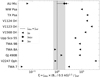 |
Fig. 10. Ratio of the observed to predicted SAM jobs/jfinal. To facilitate the comparison, jobs is multiplied by a factor of (B⋆/0.5 kG)1.1 (see text). The vertical dashed line indicates a perfect agreement between the observed value and our model jref(M⋆). The gray area accounts for different stellar and disk parameters. The SAM values jBI and jBV are based on BI and BV functions as the upper and lower boundary for the stellar SAM. They are indicated by left and right-facing triangles, respectively. The single measured value (and uncertainties) of jBQU (diamond marker) is based on BQU for the star AU Mic. The measurements are tabulated in Table C.1. |
4.3. Accretion-powered stellar wind (APSW) efficiency W
Winds, in this study represented by APSW, can strongly affect the distribution of stellar SAM as well as the structure and long-term evolution of its disk (e.g., Matt & Pudritz 2005a; Gallet et al. 2019). APSW is a potential explanation for the existence of slowly spinning stars, but their exact mechanisms and strength are the subject of active research (see the discussion in Gallet et al. 2019). Observations of Doppler-shifted line absorption features (Dupree et al. 2005; Edwards et al. 2006) as well as statistical evaluations of the observed ratio of outflow mass loss to disk accretion rate (e.g., Cabrit 2002; Ferreira et al. 2006) indicate that there are indeed strong outflows from young star-disk systems. These outflows are expected to be too cool to originate from a thermal pressure gradient at the stellar corona where temperatures are ∼106 K (e.g., Gallet et al. 2019) and their exact launch point and driving mechanism are not known (e.g., Ireland et al. 2021) but they are supposed to be disk winds launched in the inner disk, possibly by the magneto-centrifugal process (e.g., Königl et al. 2011); some of these winds can even form jets. A possible alternative driving mechanism for winds is proposed in Decampli (1981) and Matt & Pudritz (2005a). The accreting disk material can excite Alfvén waves originating at the stellar surface, traveling outward and removing angular momentum from the star. The mass loss rate through these winds is expected to be W ∼ 2% (Cranmer 2008; Pantolmos et al. 2020).
While previous authors need large APSW values of ∼10% to explain slowly spinning stars, which contradicts the results of Cranmer (2008) and Pantolmos et al. (2020), we can reduce this value considerably to reproduce the observed rotational period of slowly rotating stars. In this work, we can limit W to ≲5%, which is in better agreement with observational constraints and consistent with the theoretical predictions of Cranmer (2008) and Pantolmos et al. (2020). The reduction of W might be explained by the combined stellar and disk model that includes the back-reactions of the rotational evolution on the accretion disk and the spin-down effect of MEs, especially during phases of fast stellar rotation and toward the end of the disk lifetime. Apart from APSW and MEs, other wind mechanisms can be important for star and disk evolution. Especially, disk winds noticeably affect the disk evolution (e.g., Königl et al. 2011). By removing mass and (if magnetized) angular momentum from the disk before it can be accreted onto the star, the evolution of stellar spin evolution is affected. Likewise, photo-evaporation (internal or external) can influence the disk’s lifetime and thus, the stellar spin evolution (e.g., Roquette et al. 2021). These effects will be added to a future version of our model.
4.4. Comparing our model to large-scale parametric studies
Our model predictions can be directly integrated into parametric-based modeling of the stellar spin evolution of young stars, including the influence of an accretion disk (e.g., Vasconcelos & Bouvier 2017). While Vasconcelos & Bouvier (2017) have conducted a large number of simulations (∼2 × 10⁵), exceeding the number of our simulations by over two orders of magnitude, their model is parametric and the evolution of the accretion disk and the star-disk interaction is based on simplified assumptions. The disk accretion rate is taken to be independent of stellar mass and the disk lifetime is estimated based on a free parameter. During the disk lifetime, disk-locking is assumed (the stellar rotational period is constant over time) and important aspects like the influence of a stellar magnetic field or an accretion-powered stellar wind are ignored.
Vasconcelos & Bouvier (2017) can present useful guidelines regarding the rotational evolution of low-mass stars. However, none of their models can reproduce all the available observational aspects (e.g., a correlation between stellar mass and rotation period). We can provide mass-dependent disk lifetimes for different disk parameters (e.g., Fig. 3) and a relation for the SAM after the disk phase that includes the influence of the stellar magnetic field strength and an accretion-powered stellar wind (Eq. (6)). Combining our results with the method presented in Vasconcelos & Bouvier (2017), could lead to new constraints for stellar and disk parameters (e.g., the mass-dependent distribution of stellar magnetic strength or mass-dependent APSW efficiency).
5. Conclusion and caveats
To investigate the factors that govern the angular momentum distribution of young M dwarfs, we ran more than 500 long-term (up to 10 Myr) simulations of a rotating star and disk and the interaction between them in the innermost disk (≲0.05 AU). This large number of simulations, spanning a wide parameter space, was possible due to the implicit solver in the code, which circumvents the limitations of using explicit time steps when simulating disk physics on both small (inner edge) and large (outer edge) scales. Our model includes physics in a more self-consistent manner (e.g., pressure gradients and magnetic torques in the inner disk, deviations from the Keplerian velocity or the back-reaction in the disk) compared to previous long-term simulations (e.g., Matt et al. 2010; Gallet et al. 2019).
The main conclusions of this work are:
-
If the initial accretion rate (a proxy for disk mass) is above a critical value Ṁcrit ∼ 10−8 M⊙ yr−1, the accretion disk effectively “erases” the initial spin of the star and the spin and angular momentum (AM) evolves in a convergent manner that is independent of the initial AM. In such cases, the final SAM (SAM) is controlled by stellar and disk parameters, M⋆, B⋆, α, and W. Consistent with Armitage & Clarke (1996), we find that sufficiently massive disks can regulate stellar rotation.
-
For stellar masses > 0.3 M⊙, the initial accretion rates Ṁinit at ∼1 Myr are comparable to Ṁcrit. The SAM of these young M dwarfs after the disk phase jfinal is independent of the initial conditions and scales with the stellar magnetic field strength as
 . For stellar masses ≲0.3 M⊙, Ṁinit < Ṁcrit and the initial stellar rotation periods affect the SAM after the disk phase.
 -
Stellar dipole field strengths in the range of ∼30 G to ∼1 kG (see Fig. 9) are necessary to reproduce the nearly mass-independent SAM distribution reported by Somers et al. (2017) with higher stellar masses requiring stronger field strengths. These results match the range of observed large-scale dipole field strengths reported in the literature. In addition, the positive relation between the stellar mass and the magnetic field strength is needed to explain the mass-independent SAM distribution in the presence of mass-dependent accretion rates and is suggested by theoretical scaling arguments (Browning et al. 2016).
-
Our scaling relation is also consistent with (but not robustly tested by) the few available observations of SAM, mass, and magnetic field strength in individual stars.
Our study points to future directions in advancement in both modeling and observations but should be considered preliminary because of important caveats and limitations of our model. Model dimensionality: Our one-dimensional model does not resolve the vertical structure of the disk or include vertical gradients as shear. Thus, certain mechanisms such as for example vertical shear instabilities (e.g., Urpin & Brandenburg 1998; Nelson et al. 2013; Latter & Kunz 2022) and vertically resolved “dead” zones (e.g., Jankovic et al. 2021; Delage et al. 2022) which could be important for the transport of mass and angular momentum cannot be included. An expansion to two dimensions, including the vertical dimension, would allow such phenomena to be included. Early disk evolution: Phenomena relevant to the earlier (≲1 Myr) phase (Class 0 and Class 1 phases) of stellar evolution of the star-disk system are not included in the TAPIR code. The effects of a more massive disk, accretion outbursts, and in-falling material from the parent cloud core could be included in future studies. Vorobyov et al. (2017) show that unsteady accretion during this early phase can affect later stellar evolution. Premain sequence contraction: In the current TAPIR version the contraction of the central star is described by the simplified Kelvin-Helmholtz contraction. Due to unsteady accretion, which can occur even in later disk stages (e.g., HBC 722, Kóspál et al. 2016), the contraction can deviate significantly from the Kelvin-Helmholtz relation. A future improvement could be combining the TAPIR code with the predictions of a full stellar evolution code (e.g., MESA Paxton et al. 2019). The combination of a stellar evolution code with our current model would further allow a more self-consistent treatment of the evolution of the stellar magnetic field strength, assuming the magnetic energy density scales with the kinetic energy of the convective flow (e.g., Browning et al. 2016). Stellar multiplicity: in the current study, we only consider single stars. Binary or multiple systems tend to influence the evolution of the accretion disk (e.g., Akeson et al. 2019; Zagaria et al. 2021). The influence of a binary companion on the angular momentum of a star will be studied in future work. Transport of mass and angular momentum: Our model relies on a simple (constant α-parameter) prescription for viscous transport of mass and angular momentum in the disk. α is almost certainly not constant with time and location in the disk, and other mechanisms such as disk winds and photo-evaporation, which cannot be described with this parameterization, are important for disk evolution (e.g., Königl et al. 2011; Roquette et al. 2021). These are currently not included but could, in principle, be added in some future version of our model.
We refer to the sharp drop in rotation periods at ∼15 days in Fig. 19 of Rebull et al. (2015).
Acknowledgments
The authors thank the anonymous referees for providing comments and suggestions that helped to improve the quality of this work. The authors thank Ansgar Reiners for the discussion of measurements of stellar magnetic fields. E.G. acknowledges a 2021 Ida Pfeiffer Professorship in the Faculty of Earth Sciences, Geography, and Astronomy at the University of Vienna, and support from NSF Astronomy & Astrophysics grant 1817215.
References
- Affer, L., Micela, G., Favata, F., Flaccomio, E., & Bouvier, J. 2013, MNRAS, 430, 1433 [Google Scholar]
- Akeson, R. L., Jensen, E. L. N., Carpenter, J., et al. 2019, ApJ, 872, 158 [Google Scholar]
- Alonso-Martínez, M., Riviere-Marichalar, P., Meeus, G., et al. 2017, A&A, 603, A138 [EDP Sciences] [Google Scholar]
- Armitage, P. J. 2013, Astrophysics of Planet Formation (Cambridge: Cambridge University Press) [Google Scholar]
- Armitage, P. J., & Clarke, C. J. 1996, MNRAS, 280, 458 [NASA ADS] [Google Scholar]
- Armitage, P. J., Livio, M., & Pringle, J. E. 2001, MNRAS, 324, 705 [NASA ADS] [CrossRef] [Google Scholar]
- Bai, X.-N., & Stone, J. M. 2013, ApJ, 769, 76 [Google Scholar]
- Baraffe, I., Homeier, D., Allard, F., & Chabrier, G. 2015, A&A, 577, A42 [NASA ADS] [CrossRef] [EDP Sciences] [Google Scholar]
- Barnes, S. A. 2007, ApJ, 669, 1167 [Google Scholar]
- Bessolaz, N., Zanni, C., Ferreira, J., Keppens, R., & Bouvier, J. 2008, A&A, 478, 155 [NASA ADS] [CrossRef] [EDP Sciences] [Google Scholar]
- Bouvier, J., Matt, S. P., Mohanty, S., et al. 2014, in Protostars and Planets VI, eds. H. Beuther, R. S. Klessen, C. P. Dullemond, & T. Henning, 433 [Google Scholar]
- Browning, M. K., Weber, M. A., Chabrier, G., & Massey, A. P. 2016, ApJ, 818, 189 [NASA ADS] [CrossRef] [Google Scholar]
- Buccino, A. P., Lemarchand, G. A., & Mauas, P. J. D. 2006, Icarus, 183, 491 [NASA ADS] [CrossRef] [Google Scholar]
- Cabrit, S. 2002, in EAS Publications Series, eds. J. Bouvier, & J. P. Zahn, 3, 147 [NASA ADS] [CrossRef] [EDP Sciences] [Google Scholar]
- Caratti o Garatti, A., Garcia Lopez, R., Antoniucci, S., et al. 2012, A&A, 538, A64 [NASA ADS] [CrossRef] [EDP Sciences] [Google Scholar]
- Cecchi-Pestellini, C., Ciaravella, A., Micela, G., & Penz, T. 2009, A&A, 496, 863 [NASA ADS] [CrossRef] [EDP Sciences] [Google Scholar]
- Chabrier, G. 2003, PASP, 115, 763 [Google Scholar]
- Claytor, Z. R., van Saders, J. L., Llama, J., et al. 2022, ApJ, 927, 219 [NASA ADS] [CrossRef] [Google Scholar]
- Cody, A. M., & Hillenbrand, L. A. 2010, ApJS, 191, 389 [NASA ADS] [CrossRef] [Google Scholar]
- Collier Cameron, A., & Campbell, C. G. 1993, A&A, 274, 309 [NASA ADS] [Google Scholar]
- Courant, R., Friedrichs, K., & Lewy, H. 1928, Math. Ann., 100, 32 [Google Scholar]
- Cranmer, S. R. 2008, ApJ, 689, 316 [NASA ADS] [CrossRef] [Google Scholar]
- Decampli, W. M. 1981, ApJ, 244, 124 [NASA ADS] [CrossRef] [Google Scholar]
- Delage, T. N., Okuzumi, S., Flock, M., Pinilla, P., & Dzyurkevich, N. 2022, A&A, 658, A97 [NASA ADS] [CrossRef] [EDP Sciences] [Google Scholar]
- Donati, J.-F., Skelly, M. B., Bouvier, J., et al. 2010, MNRAS, 402, 1426 [Google Scholar]
- Dorfi, E., & Drury, L. 1987, J. Comput. Phys., 69, 175 [NASA ADS] [CrossRef] [Google Scholar]
- Douglas, S. T., Agüeros, M. A., Covey, K. R., & Kraus, A. 2017, ApJ, 842, 83 [Google Scholar]
- Douglas, S. T., Curtis, J. L., Agüeros, M. A., et al. 2019, ApJ, 879, 100 [Google Scholar]
- Dupree, A. K., Brickhouse, N. S., Smith, G. H., & Strader, J. 2005, ApJ, 625, L131 [CrossRef] [Google Scholar]
- Edwards, S., Fischer, W., Hillenbrand, L., & Kwan, J. 2006, ApJ, 646, 319 [Google Scholar]
- Feiden, G. A. 2016, A&A, 593, A99 [NASA ADS] [CrossRef] [EDP Sciences] [Google Scholar]
- Ferreira, J., Pelletier, G., & Appl, S. 2000, MNRAS, 312, 387 [NASA ADS] [CrossRef] [Google Scholar]
- Ferreira, J., Dougados, C., & Cabrit, S. 2006, A&A, 453, 785 [NASA ADS] [CrossRef] [EDP Sciences] [Google Scholar]
- Finley, A. J., & Matt, S. P. 2018, ApJ, 854, 78 [Google Scholar]
- Fiorellino, E., Manara, C. F., Nisini, B., et al. 2021, A&A, 650, A43 [NASA ADS] [CrossRef] [EDP Sciences] [Google Scholar]
- Fiorellino, E., Tychoniec, Ł., Manara, C. F., et al. 2022, ApJ, 937, L9 [NASA ADS] [CrossRef] [Google Scholar]
- Folsom, C. P., Petit, P., Bouvier, J., et al. 2016, MNRAS, 457, 580 [Google Scholar]
- France, K., Froning, C. S., Linsky, J. L., et al. 2013, ApJ, 763, 149 [Google Scholar]
- France, K., Arulanantham, N., Fossati, L., et al. 2018, ApJS, 239, 16 [Google Scholar]
- Gallet, F., & Bouvier, J. 2013, A&A, 556, A36 [NASA ADS] [CrossRef] [EDP Sciences] [Google Scholar]
- Gallet, F., Zanni, C., & Amard, L. 2019, A&A, 632, A6 [NASA ADS] [CrossRef] [EDP Sciences] [Google Scholar]
- Ghosh, P., & Lamb, F. K. 1979, ApJ, 234, 296 [Google Scholar]
- Güdel, M., Guinan, E. F., & Skinner, S. L. 1997, ApJ, 483, 947 [Google Scholar]
- Güdel, M., Briggs, K. R., Arzner, K., et al. 2007, A&A, 468, 353 [Google Scholar]
- Güdel, M., Eibensteiner, C., Dionatos, O., et al. 2018, A&A, 620, L1 [NASA ADS] [CrossRef] [EDP Sciences] [Google Scholar]
- Hartman, J. D., Gaudi, B. S., Pinsonneault, M. H., et al. 2009, ApJ, 691, 342 [Google Scholar]
- Herbst, W., Bailer-Jones, C. A. L., Mundt, R., Meisenheimer, K., & Wackermann, R. 2002, A&A, 396, 513 [EDP Sciences] [Google Scholar]
- Hill, C. A., Folsom, C. P., Donati, J.-F., et al. 2019, MNRAS, 484, 5810 [Google Scholar]
- Howard, W. S., Teske, J., Corbett, H., et al. 2021, AJ, 162, 147 [NASA ADS] [CrossRef] [Google Scholar]
- Howell, S. B., Sobeck, C., Haas, M., et al. 2014, PASP, 126, 398 [Google Scholar]
- Ireland, L. G., Zanni, C., Matt, S. P., & Pantolmos, G. 2021, ApJ, 906, 4 [Google Scholar]
- Irwin, J., & Bouvier, J. 2009, in The Ages of Stars, eds. E. E. Mamajek, D. R. Soderblom, & R. F. G. Wyse, 258, 363 [Google Scholar]
- Irwin, J., Hodgkin, S., Aigrain, S., et al. 2008, MNRAS, 384, 675 [CrossRef] [Google Scholar]
- Jankovic, M. R., Owen, J. E., Mohanty, S., & Tan, J. C. 2021, MNRAS, 504, 280 [NASA ADS] [CrossRef] [Google Scholar]
- Johnstone, C. P., Jardine, M., Gregory, S. G., Donati, J. F., & Hussain, G. 2014, MNRAS, 437, 3202 [Google Scholar]
- Klutsch, A., Freire Ferrero, R., Guillout, P., et al. 2014, A&A, 567, A52 [NASA ADS] [CrossRef] [EDP Sciences] [Google Scholar]
- Kluźniak, W., & Rappaport, S. 2007, ApJ, 671, 1990 [CrossRef] [Google Scholar]
- Kochukhov, O. 2021, A&ARv, 29, 1 [Google Scholar]
- Kochukhov, O., & Reiners, A. 2020, ApJ, 902, 43 [Google Scholar]
- Koenigl, A. 1991, ApJ, 370, L39 [Google Scholar]
- Königl, A., Romanova, M. M., & Lovelace, R. V. E. 2011, MNRAS, 416, 757 [NASA ADS] [Google Scholar]
- Kóspál, Á., Ábrahám, P., Acosta-Pulido, J. A., et al. 2016, A&A, 596, A52 [NASA ADS] [CrossRef] [EDP Sciences] [Google Scholar]
- Lammer, H., Selsis, F., Ribas, I., et al. 2003, ApJ, 598, L121 [Google Scholar]
- Latter, H. N., & Kunz, M. W. 2022, MNRAS, 511, 1182 [CrossRef] [Google Scholar]
- Lavail, A., Kochukhov, O., & Hussain, G. A. J. 2019, A&A, 630, A99 [NASA ADS] [CrossRef] [EDP Sciences] [Google Scholar]
- Lecavelier Des Etangs, A., Ehrenreich, D., Vidal-Madjar, A., et al. 2010, A&A, 514, A72 [NASA ADS] [CrossRef] [EDP Sciences] [Google Scholar]
- Mamajek, E. E. 2009, in Exoplanets and Disks: Their Formation and Diversity, eds. T. Usuda, M. Tamura, & M. Ishii, AIP Conf. Ser., 1158, 3 [NASA ADS] [CrossRef] [Google Scholar]
- Manara, C. F., Robberto, M., Rio, N. D., et al. 2012, ApJ, 755, 154 [NASA ADS] [CrossRef] [Google Scholar]
- Manara, C. F., Ansdell, M., Rosotti, G. P., et al. 2022, arXiv e-prints [arXiv:2203.09930] [Google Scholar]
- Matt, S., & Pudritz, R. E. 2005a, ApJ, 632, L135 [Google Scholar]
- Matt, S., & Pudritz, R. E. 2005b, MNRAS, 356, 167 [NASA ADS] [CrossRef] [Google Scholar]
- Matt, S., & Pudritz, R. E. 2008a, ApJ, 678, 1109 [NASA ADS] [CrossRef] [Google Scholar]
- Matt, S., & Pudritz, R. E. 2008b, ApJ, 681, 391 [Google Scholar]
- Matt, S. P., Pinzón, G., de la Reza, R., & Greene, T. P. 2010, ApJ, 714, 989 [NASA ADS] [CrossRef] [Google Scholar]
- Matt, S. P., Pinzón, G., Greene, T. P., & Pudritz, R. E. 2012, ApJ, 745, 101 [NASA ADS] [CrossRef] [Google Scholar]
- Matt, S. P., Brun, A. S., Baraffe, I., Bouvier, J., & Chabrier, G. 2015, ApJ, 799, L23 [Google Scholar]
- Meibom, S., Barnes, S. A., Latham, D. W., et al. 2011, ApJ, 733, L9 [Google Scholar]
- Messina, S., Santallo, R., Tan, T. G., et al. 2017, A&A, 601, A54 [NASA ADS] [CrossRef] [EDP Sciences] [Google Scholar]
- Micela, G., Sciortino, S., Serio, S., et al. 1985, ApJ, 292, 172 [CrossRef] [Google Scholar]
- Nelson, R. P., Gressel, O., & Umurhan, O. M. 2013, MNRAS, 435, 2610 [Google Scholar]
- Nicholson, B. A., Hussain, G., Donati, J. F., et al. 2021, MNRAS, 504, 2461 [NASA ADS] [CrossRef] [Google Scholar]
- Nortmann, L., Pallé, E., Salz, M., et al. 2018, Science, 362, 1388 [Google Scholar]
- Pallavicini, R., Golub, L., Rosner, R., et al. 1981, ApJ, 248, 279 [NASA ADS] [CrossRef] [Google Scholar]
- Pantolmos, G., Zanni, C., & Bouvier, J. 2020, A&A, 643, A129 [NASA ADS] [CrossRef] [EDP Sciences] [Google Scholar]
- Paxton, B., Smolec, R., Schwab, J., et al. 2019, ApJS, 243, 10 [Google Scholar]
- Pfalzner, S., Dehghani, S., & Michel, A. 2022, ApJ, 939, L10 [NASA ADS] [CrossRef] [Google Scholar]
- Phan-Bao, N., Lim, J., Donati, J.-F., Johns-Krull, C. M., & Martín, E. L. 2009, ApJ, 704, 1721 [NASA ADS] [CrossRef] [Google Scholar]
- Pizzolato, N., Maggio, A., Micela, G., Sciortino, S., & Ventura, P. 2003, A&A, 397, 147 [NASA ADS] [CrossRef] [EDP Sciences] [Google Scholar]
- Plavchan, P., Barclay, T., Gagné, J., et al. 2020, Nature, 582, 497 [Google Scholar]
- Pringle, J. E. 1981, ARA&A, 19, 137 [NASA ADS] [CrossRef] [Google Scholar]
- Ragossnig, F., Dorfi, E. A., Ratschiner, B., et al. 2020, Comput. Phys. Commun., 256, 107437 [NASA ADS] [CrossRef] [Google Scholar]
- Rappaport, S. A., Fregeau, J. M., & Spruit, H. 2004, ApJ, 606, 436 [NASA ADS] [CrossRef] [Google Scholar]
- Rebull, L. M., Stauffer, J. R., Megeath, S. T., Hora, J. L., & Hartmann, L. 2006, ApJ, 646, 297 [NASA ADS] [CrossRef] [Google Scholar]
- Rebull, L. M., Padgett, D. L., McCabe, C. E., et al. 2010, ApJS, 186, 259 [NASA ADS] [CrossRef] [Google Scholar]
- Rebull, L. M., Stauffer, J. R., Cody, A. M., et al. 2015, AJ, 150, 175 [NASA ADS] [CrossRef] [Google Scholar]
- Rebull, L. M., Stauffer, J. R., Bouvier, J., et al. 2016, AJ, 152, 113 [Google Scholar]
- Rebull, L. M., Stauffer, J. R., Hillenbrand, L. A., et al. 2017, ApJ, 839, 92 [Google Scholar]
- Rebull, L. M., Stauffer, J. R., Cody, A. M., et al. 2018, AJ, 155, 196 [Google Scholar]
- Rebull, L. M., Stauffer, J. R., Cody, A. M., et al. 2020, AJ, 159, 273 [Google Scholar]
- Reiners, A., Basri, G., & Christensen, U. R. 2009, ApJ, 697, 373 [NASA ADS] [CrossRef] [Google Scholar]
- Reiners, A., Shulyak, D., Käpylä, P. J., et al. 2022, A&A, 662, A41 [NASA ADS] [CrossRef] [EDP Sciences] [Google Scholar]
- Ribas, Á., Espaillat, C. C., Macías, E., & Sarro, L. M. 2020, A&A, 642, A171 [NASA ADS] [CrossRef] [EDP Sciences] [Google Scholar]
- Richert, A. J. W., Getman, K. V., Feigelson, E. D., et al. 2018, MNRAS, 477, 5191 [NASA ADS] [CrossRef] [Google Scholar]
- Romanova, M., & Kurosawa, R. 2014, in 8th International Conference of Numerical Modeling of Space Plasma Flows (ASTRONUM 2013), eds. N. V. Pogorelov, E. Audit, & G. P. Zank, ASP Conf. Ser., 488, 127 [Google Scholar]
- Romanova, M. M., Ustyugova, G. V., Koldoba, A. V., & Lovelace, R. V. E. 2002, ApJ, 578, 420 [Google Scholar]
- Romanova, M. M., Ustyugova, G. V., Koldoba, A. V., & Lovelace, R. V. E. 2004, ApJ, 610, 920 [Google Scholar]
- Romanova, M. M., Ustyugova, G. V., Koldoba, A. V., & Lovelace, R. V. E. 2009, MNRAS, 399, 1802 [Google Scholar]
- Roquette, J., Matt, S. P., Winter, A. J., Amard, L., & Stasevic, S. 2021, MNRAS, 508, 3710 [NASA ADS] [CrossRef] [Google Scholar]
- Sanz-Forcada, J., Micela, G., Ribas, I., et al. 2011, A&A, 532, A6 [NASA ADS] [CrossRef] [EDP Sciences] [Google Scholar]
- Serna, J., Hernandez, J., Kounkel, M., et al. 2021, ApJ, 923, 177 [NASA ADS] [CrossRef] [Google Scholar]
- Shakura, N., & Sunyaev, R. 1973, A&A, 24, 337 [Google Scholar]
- Shu, F., Najita, J., Ostriker, E., et al. 1994, ApJ, 429, 781 [Google Scholar]
- Sicilia-Aguilar, A., Banzatti, A., Carmona, A., et al. 2016, PASA, 33, e059 [NASA ADS] [CrossRef] [Google Scholar]
- Somers, G., Stauffer, J., Rebull, L., Cody, A. M., & Pinsonneault, M. 2017, ApJ, 850, 134 [NASA ADS] [CrossRef] [Google Scholar]
- Steiner, D., Gehrig, L., Ratschiner, B., et al. 2021, A&A, 655, A110 [NASA ADS] [CrossRef] [EDP Sciences] [Google Scholar]
- Testi, L., Natta, A., Manara, C. F., et al. 2022, A&A, 663, A98 [NASA ADS] [CrossRef] [EDP Sciences] [Google Scholar]
- Tobin, J. J., Sheehan, P. D., Megeath, S. T., et al. 2020, ApJ, 890, 130 [CrossRef] [Google Scholar]
- Urpin, V., & Brandenburg, A. 1998, MNRAS, 294, 399 [Google Scholar]
- Vasconcelos, M. J., & Bouvier, J. 2017, A&A, 600, A116 [NASA ADS] [CrossRef] [EDP Sciences] [Google Scholar]
- Venuti, L., Bouvier, J., Cody, A. M., et al. 2017, A&A, 599, A23 [NASA ADS] [CrossRef] [EDP Sciences] [Google Scholar]
- Vorobyov, E. I., & Basu, S. 2009, MNRAS, 393, 822 [CrossRef] [Google Scholar]
- Vorobyov, E. I., Elbakyan, V., Hosokawa, T., et al. 2017, A&A, 605, A77 [NASA ADS] [CrossRef] [EDP Sciences] [Google Scholar]
- Vorobyov, E. I., Khaibrakhmanov, S., Basu, S., & Audard, M. 2020, A&A, 644, A74 [NASA ADS] [CrossRef] [EDP Sciences] [Google Scholar]
- Wright, N. J., Drake, J. J., Mamajek, E. E., & Henry, G. W. 2011, ApJ, 743, 48 [Google Scholar]
- Yang, H., & Johns-Krull, C. M. 2011, ApJ, 729, 83 [Google Scholar]
- Yang, H., Johns-Krull, C. M., & Valenti, J. A. 2008, AJ, 136, 2286 [NASA ADS] [CrossRef] [Google Scholar]
- Yang, C.-C., Mac Low, M.-M., & Johansen, A. 2018, ApJ, 868, 27 [NASA ADS] [CrossRef] [Google Scholar]
- Zagaria, F., Rosotti, G. P., & Lodato, G. 2021, MNRAS, 507, 2531 [NASA ADS] [CrossRef] [Google Scholar]
- Zanni, C., & Ferreira, J. 2013, A&A, 550, A99 [NASA ADS] [CrossRef] [EDP Sciences] [Google Scholar]
- Zechmeister, M., Kürster, M., & Endl, M. 2009, A&A, 505, 859 [NASA ADS] [CrossRef] [EDP Sciences] [Google Scholar]
- Zhu, Z., Hartmann, L., Calvet, N., et al. 2007, ApJ, 669, 483 [NASA ADS] [CrossRef] [Google Scholar]
- Zhu, Z., Hartmann, L., Gammie, C. F., et al. 2010, ApJ, 713, 1134 [Google Scholar]
Appendix A: Influence of MEs for different configurations
The torque due to magnetospheric ejections (MEs) is shown for different configurations in Fig. A.1 compared to a reference model. The reference model (solid black line) has a magnetic field strength of B⋆ = 0.5 kG, an initial rotation period of Pinit = 10 days, an initial accretion rate of Ṁinit = 1 × 10⁻⁸ M⊙ yr−1, a viscosity parameter α = 0.01, and a stellar mass of M⋆ = 0.3 M⊙. We increase the strength of the magnetic field to B⋆ = 1.0 kG (model "B⋆high", solid red line), decrease the initial rotation period to 1 day (model "Pinitfast", solid blue line), and reduce the initial accretion rate to Ṁinit = 3 × 10⁻⁹ M⊙ yr−1 (model "Ṁinitlow", solid yellow line). The transfer between the spin-up and spin-down regime is marked with a horizontal black dashed line. For comparison, the spin-down torque due to the APSW, ΓW, for model B⋆high is shown as a dashed red line.
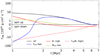 |
Fig. A.1. Evolution of the torque due to magnetospheric ejections (MEs) for different configurations (see text). The transfer between the spin-up and spin-down regime is marked with a horizontal black dashed line. For comparison, the spin-down torque due to the APSW, ΓW, for model B⋆high is shown as a dashed red line. |
Appendix B: Flat spectrum sources
Observed accretion rates of flat spectrum sources used in Fig. 3.
Stellar masses and accretion rates of flat-spectrum sources with M⋆ < 1 M⊙ used in Fig. 3. In addition, the method for determining the accretion rate (MethodṀ⋆) is given. If only one reference is given it contains stellar mass and the accretion rate.
Appendix C: Observational data for stars after the disk phase
Stellar observational data used in Fig. 9 and Fig. 10 is shown in Table C.1.
Stellar observational data used in Fig. 9 and Fig. 10. The respective uncertainties are given when available. Missing data is represented by "—".
All Tables
Stellar masses and accretion rates of flat-spectrum sources with M⋆ < 1 M⊙ used in Fig. 3. In addition, the method for determining the accretion rate (MethodṀ⋆) is given. If only one reference is given it contains stellar mass and the accretion rate.
Stellar observational data used in Fig. 9 and Fig. 10. The respective uncertainties are given when available. Missing data is represented by "—".
All Figures
|
Fig. 1. Schematic cartoon of inner disk-star connection. The star (black quarter circle on the left) has a radius of R⋆ and rotates with Ω⋆. Disk material (gray area) flows from the outer disk toward the inner disk radius rin, where it is forced into funnel flows and is accreted onto the star (e.g., Romanova et al. 2004; Bessolaz et al. 2008; Steiner et al. 2021) with an accretion rate of ṀW. The accreted disk material increases the stellar angular momentum by Γacc. Based on the model, a specific fraction of the accreted mass is driven into a stellar wind, which removes mass and angular momentum from the star (Ṁref and ΓW, respectively). The Alfvén radius rA acts as a lever arm for this stellar outflow. We note that this cartoon is not to scale and we can usually assume rA ≫ R⋆. Angular momentum can be transferred toward or away from the star (ΓME), depending on the position of rin with respect to the corotation radius rcor (e.g., Zanni & Ferreira 2013). Finally, magneto-centrifugally driven disk winds remove angular momentum and mass from the disk before it can be accreted on the star (e.g., Königl et al. 2011; Bai & Stone 2013). We note that disk winds are not included in our model. |
| In the text | |
|
Fig. 2. Distribution of stellar rotation periods in young clusters: ONC (R+06, Rebull et al. 2006), σ Ori (C+H10, Cody & Hillenbrand 2010), NGC 2264 (V+17, Venuti et al. 2017), Taurus (R+20, Rebull et al. 2020) and the Orion star forming region (S+21, Serna et al. 2021). |
| In the text | |
|
Fig. 3. Observed accretion rates of Class I (gray), Class II (red), and flat spectrum (blue) sources. The gray dash-dotted line is taken from Fiorellino et al. (2021) and the gray dotted line from Caratti o Garatti et al. (2012). The gray-shaded area is limited by the two lines. The red dashed, dotted, and dash-dotted lines are taken from Manara et al. (2012), Fiorellino et al. (2021), and Testi et al. (2022), respectively. The red-shaded area has a minimum but constant logarithmic height so that all red lines are comprised. The thick gray and red lines indicate the mean values of the Class I and Class II objects. The blue squares represent accretion rates of flat spectrum sources (summarized in Table B.1). The blue line is the best fit for the flat spectrum objects and the dashed line is five times less than that, just above the Class II regime. |
| In the text | |
|
Fig. 4. Model disk accretion rates vs. time for two cases: The Ṁex(1)(t) (blue line) and Ṁex(2)(t) (red line) cases are simulations of stars with M⋆ = 0.3 (0.1) M⊙ and a disk with a viscosity parameter α = 0.005 (0.010), respectively. The stellar magnetic field strength is the same (B⋆ = 1.0 kG) in both cases. We compare these to empirical relations based on the power-law relation Ṁ ∝ t−χ of Gallet et al. (2019) with disk lifetimes of 3.5 and 7.2 Myr and exponents χ = 1.2 (solid black line) and χ = 1.5 (dashed black line) (Vasconcelos & Bouvier 2017; Gallet et al. 2019). |
| In the text | |
|
Fig. 5. Final stellar rotation period Pfinal for different initial periods Pinit and disk accretion rates Ṁinit. The stellar and disk parameters are: B⋆ = 1000 G, M⋆ = 0.3 M⊙, W = 2% and α = 0.01. We can divide the parameter space into three different regions, separated by red lines (see text). |
| In the text | |
|
Fig. 6. C-parameter (the gradient of the contours in Fig. 5) with respect to initial disk accretion rates Ṁinit. The solid lines represent CP and the dashed lines Cj values, respectively. Each subplot shows variations in (a) viscous α parameter: 0.01 (blue lines) and 0.005 (black lines). The stellar mass is 0.3 M⊙ with a magnetic dipole field strength of B⋆ = 1 kG. (b) W values: 2% (blue lines) and 5% (black lines). The stellar mass is 0.3 M⊙ with a magnetic dipole field strength of B⋆ = 1 kG and a viscosity parameter of α = 0.01. (c) B⋆ values: 1.0 kG (blue lines) and 0.5 kG (black lines). The stellar mass is 0.3 M⊙ with a viscosity parameter of α = 0.01. (d) M⋆ values: 0.3 M⊙ (blue lines) and 0.6 M⊙ (black lines). The viscosity parameter is α = 0.01. The threshold of C = 0.01 for the star to be in the “locked”-state is indicated by the horizontal dotted line. For better visualization, the highlighted parameters show the reference value in the other subplots. |
| In the text | |
|
Fig. 7. The SAM after the disk phase jfinal for different stellar magnetic field values and stellar masses of 0.1 M⊙ (panel a), 0.3 M⊙ (panel b), and 0.5 M⊙ (panel c). The colored circles, crosses, and squares represent initial rotation periods of 1, 3, and 10 days, respectively, and the solid, dash-dotted, and dashed lines show the respective fits. Mean and standard deviation values for the SAM taken from Somers et al. (2017) are represented by gray solid and dashed lines, respectively. |
| In the text | |
|
Fig. 8. The SAM after the disk phase jfinal as a function of stellar magnetic field values (x-axis and colors) and for different initial rotation periods (different sets of point styles and curves). Each panel shows the variation of one parameter with respect to the reference case in Fig. 7. In panel a, Ṁlow is used as the initial accretion rate. In panels b and c, the APSW efficiency is set to 0% and 5%, respectively. In panel d, the viscous α parameter is set to 0.005. In all cases, the stellar mass is 0.3 M⊙. The symbols and lines are identical to Fig. 7. For comparison, the yellow lines show the fits from Fig. 7 for a stellar mass of 0.3 M⊙. |
| In the text | |
|
Fig. 9. Observed dipole field strengths of young stars with respect to stellar mass. Solid black circles show dipole field strengths inferred by the Stokes V parameter (BV), open circles indicate an estimate based on the total field intensity (BI) and a dipole field strength fraction of blsf = 22% (Lavail et al. 2019), and the black diamond indicates the dipole field strength of AU Mic, the only young star in our sample with direct measurement of BQU. The errors are expected to reach up to one order of magnitude. The range of the required magnetic field strengths to match the observed median value of the SAM distribution (Somers et al. 2017) is marked in blue ( |
| In the text | |
|
Fig. 10. Ratio of the observed to predicted SAM jobs/jfinal. To facilitate the comparison, jobs is multiplied by a factor of (B⋆/0.5 kG)1.1 (see text). The vertical dashed line indicates a perfect agreement between the observed value and our model jref(M⋆). The gray area accounts for different stellar and disk parameters. The SAM values jBI and jBV are based on BI and BV functions as the upper and lower boundary for the stellar SAM. They are indicated by left and right-facing triangles, respectively. The single measured value (and uncertainties) of jBQU (diamond marker) is based on BQU for the star AU Mic. The measurements are tabulated in Table C.1. |
| In the text | |
|
Fig. A.1. Evolution of the torque due to magnetospheric ejections (MEs) for different configurations (see text). The transfer between the spin-up and spin-down regime is marked with a horizontal black dashed line. For comparison, the spin-down torque due to the APSW, ΓW, for model B⋆high is shown as a dashed red line. |
| In the text | |
Current usage metrics show cumulative count of Article Views (full-text article views including HTML views, PDF and ePub downloads, according to the available data) and Abstracts Views on Vision4Press platform.
Data correspond to usage on the plateform after 2015. The current usage metrics is available 48-96 hours after online publication and is updated daily on week days.
Initial download of the metrics may take a while.