| Issue |
A&A
Volume 696, April 2025
|
|
|---|---|---|
| Article Number | L18 | |
| Number of page(s) | 7 | |
| Section | Letters to the Editor | |
| DOI | https://doi.org/10.1051/0004-6361/202553730 | |
| Published online | 25 April 2025 | |
Letter to the Editor
Do accretion-powered stellar winds help spin down T Tauri stars?
1
Department of Astrophysics, University of Vienna, Türkenschanzstrasse 17, 1180 Vienna, Austria
2
Department of Earth Sciences, University of Hawai’i at Mānoa, Honolulu, Hawai’i 96822, USA
3
SETI Institute, 339 Bernardo Ave., Suite 200, Mountain View, CA 94043, USA
4
Visiting Fellow, School of Physics, UNSW Science, Kensington, NSW 2052, Australia
5
Jet Propulsion Laboratory, California Institute of Technology, 4800 Oak Grove Drive, Pasadena, California 91109, USA
⋆ Corresponding author: lukasg90@unet.univie.ac.at
Received:
12
January
2025
Accepted:
3
April
2025
How T Tauri stars remain slowly rotating while still accreting material is a long-standing puzzle. Current models suggest that these stars may lose angular momentum through magnetospheric ejections (MEs) of disk material and accretion-powered stellar winds (APSWs). The individual contribution of each mechanism to the stellar spin evolution, however, is also unclear. We explore how these two scenarios could be distinguished by applying stellar spin models to near-term observations. We produced synthetic stellar populations of accreting Class II stars with spreads in the parameters governing the spin-down processes and find that an APSW strongly affects the ratio of the disk truncation radius to the co-rotation radius, ℛ = Rt/Rco. The ME and APSW scenarios are distinguished to a high degree of confidence when at least Ncrit ≳ 250 stars have values measured for ℛ. Newly developed light curve analysis methods enable the measuring of ℛ for enough stars to distinguish the spin-down scenarios and will be important in the course of upcoming observing campaigns.
Key words: accretion / accretion disks / stars: protostars / stars: rotation
© The Authors 2025
 Open Access article, published by EDP Sciences, under the terms of the Creative Commons Attribution License (https://creativecommons.org/licenses/by/4.0), which permits unrestricted use, distribution, and reproduction in any medium, provided the original work is properly cited.
This article is published in open access under the Subscribe to Open model. Subscribe to A&A to support open access publication.
1. Introduction
The reason for the slow rotation of many T Tauri stars (with ages ≲10 Myr and masses ≲2 M⊙) is an unsolved problem. The addition of angular momentum (AM) from an accreting circumstellar disk plus contraction of the pre-main sequence star should lead to spin-up (e.g., Rebull et al. 2002). But surveys of star-forming regions and young clusters show the distribution of rotation periods to be little changed over the 1–10 Myr lifetime of protoplanetary disks (PPD; e.g., Rebull et al. 2006; Cody & Hillenbrand 2010; Venuti et al. 2017; Rebull et al. 2020; Serna et al. 2021; Smith et al. 2023). Most stars have rotation periods between 1 and 10 days, with a modal value of about 3–4 days. It is only after PPD dissipation that stars show the expected spin-up toward the main sequence (e.g., Gallet & Bouvier 2013).
The interaction between the star and the PPD is assumed to remove AM from the star, thus preventing spin-up (e.g., Koenigl 1991). Current stellar spin evolution models (e.g., Gallet et al. 2019; Pantolmos et al. 2020; Ireland et al. 2021, 2022) explain the loss of AM by two mechanisms. First, magnetospheric ejections (MEs; Zanni & Ferreira 2013) are the result of the relative motion of the stellar magnetic field through the partially ionized accretion disk and generate a toroidal magnetic field. The resulting additional magnetic pressure can start a cycle of inflation, reconnection, and contraction of field lines. During this cycle, some disk material is loaded onto and ejected via magnetic field lines rooted at the disk’s surface, creating a torque. The second mechanism is accretion-powered stellar winds (APSWs), where a fraction (W) of the material accreted onto the star is ejected along open stellar magnetic field lines, thus removing AM (e.g., Matt & Pudritz 2005, 2008; Matt et al. 2012; Finley & Matt 2018). Zanni & Ferreira (2011) showed that an APSW is unlikely to be the sole mechanism that spins down a T Tauri star, but the contribution of each mechanism is unclear since parameters such as W and the magnetic field strength are unknown or weakly constrained.
We used the stellar spin model of Ireland et al. (2022) to identify differences in the multiple observables of T Tauri stars due to the contribution of an APSW. We constructed a spin population model to estimate the minimum sample size of an observed distribution in order to differentiate between the no-wind (W = 0 and only MEs spin down the star) and wind scenarios (W > 0 plus MEs).
2. Spin population model
2.1. Stellar spin model
We used the model outlined in Ireland et al. (2022): Γext = ΓSDI + ΓW. Here, the external torque acting on a star consists of two components, namely, the star-disk interaction torque, ΓSDI, and the torque due to an APSW, ΓW. In the picture of ΓSDI, AM can be transferred between the star and the disk via the accretion of disk material and magnetic star-disk interaction (ME). Accreted material adds AM to the star, while the magnetic star-disk interaction adds or removes AM from the star, depending on the ratio of the truncation radius to the co-rotation radius ℛ = Rt/Rco. For ℛ < 1.0 (> 1.0), the disk’s inner edge rotates faster (slower) compared to the stellar surface. The co-rotation radius is given by Rco = (GM⋆/Ω⋆2)1/3, with the gravitational constant as G, the stellar mass as Ṁ⋆, and the stellar rotation rate as Ω⋆. The truncation radius, Rt, is where stellar magnetic forces disrupt the disk structure. Following Ireland et al. (2022), we used the expression

The disk magnetization parameter is Υacc = B⋆2R⋆2/(4πṀ⋆vesc), the fraction of the breakup speed is f, and the constants are Kt, 1 = 0.772, Kt, 2 = 1.36, Ṁ1 = 0.311, Ṁ2 = 0.0597, and Ṁ3 = −0.261. The stellar radius, magnetic field, accretion rate, and stellar escape velocity are denoted as R⋆, B⋆, and Ṁ⋆, and  . The first term in Eq. (1) is similar to the analytical expression for the truncation radius used in Bessolaz et al. (2008) or Gallet et al. (2019). The second term describes the truncation radius close to the co-rotation radius, ℛ ≈ 1. This condition can occur if Ṁ⋆ is low or B⋆ is large, for example. When Rt approaches Rco, the stellar magnetic pressure must overcome the growing disk’s thermal pressure due to a pile-up of disk material just outside Rco in addition to the ram pressure (e.g., Bessolaz et al. 2008; Steiner et al. 2021). We also required that Rt ≥ R⋆. The dependence of Rt on Ṁ⋆ is shown in Fig. 1. When approaching the co-rotation radius, the thermal pressure of the disk close to Rco slows down the decrease of Rt. The transition between the two contributions of Rt occurs at ℛ ≈ 0.7. For values of ℛ ≳ 0.7, Eq. (1) predicts significantly smaller values of Rt compared to its analytical expression. The exact position of the transition between the two regimes and the range where ℛ > 1 depend on multiple parameters, for example, B⋆, Ṁ⋆, and P⋆ (see Eq. (1)). Furthermore, specific parameter combinations, such as Ṁ⋆ ∼ 10−7 M⊙ yr−1, can lead to Rt < R⋆ and are therefore excluded from this work (as suggested in Ireland et al. 2022).
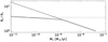 |
Fig. 1. Disk truncation radius Rt in units of stellar radius R⋆ versus accretion rate Ṁ⋆ for a 2 Myr old 0.7-M⊙ star with B⋆ = 0.5 kG and P⋆ = 2 days. The solid line shows the expression given in Eq. (1). The dashed line shows the first term of Eq. (1). The horizontal dashed line marks the co-rotation radius. In the region of Ṁ⋆ ∼ 10−7 M⊙ yr−1, the condition Rt ≥ R⋆ would be violated for the given parameters, so these values have been excluded. |
Ireland et al. (2022) divided the star-disk interaction torque ΓSDI into three states. In State 1, for ℛ < 0.433, accretion and MEs spin up the star. For values of 0.433 ≤ ℛ ≤ 1.0, accretion still spins up the star, but MEs can exert a spin-down torque (State 2). In State 3, for ℛ > 1.0, the spin-up torque due to accretion is negligible, and the MEs spin down the star. The expressions for the corresponding torques are
with the constants KSDI, 1 = 0.909 and KSDI, 2 = 0.0171. The torque due to an accretion-powered stellar wind can be written as ΓW = ṀWΩ⋆rA2 (e.g., Weber & Davis 1967) with the average Alfvén radius, rA, and the APSW mass-loss rate ṀW = WṀ⋆. We present a detailed description of the APSW torque in Appendix B. The parameter W defines the mass-loss rate of the APSW and has a magnitude of up to ∼2% (Browning et al. 2016; Pantolmos et al. 2020). We note that W does not account for the complete ejection ratio of the inner star-disk interaction region, which can reach up to ∼60% and includes processes such as APSW, MEs, and disk winds (e.g., Watson et al. 2016).
This study compares two scenarios: W = 0%, corresponding to no APSW, and W = 1%. One key parameter of the spin model is the ratio ℛ (e.g., Gallet et al. 2019; Pantolmos et al. 2020; Ireland et al. 2021, 2022). For a given star (where Ṁ⋆ and R⋆ known), Ω⋆ = 2π/P⋆ sets Rco, while Rt depends on Ṁ⋆ and B⋆. Furthermore, the value of ℛ is a measure of the rotational state of the star. For increasing values of ℛ, the spin-up (spin-down) tendency decreases (increases). Thus, P⋆, Ṁ⋆, and ℛ define the torque components and rotational properties of a given star.
2.2. Equilibrium state
As described in Ireland et al. (2022) and Mueller et al. (2024), the dependence of ΓSDI on rotation has a stabilizing effect, and it can cause an accretion disk-hosting star to evolve toward an equilibrium (or zero-torque) rotational state within a timescale of τAM = J⋆/Γext ≲ 1 − 2 Myr. Here, J⋆ is the stellar AM. An extra positive external torque causes the star to spin up, the co-rotation radius to contract, ℛ to increase, and ΓSDI to decrease. Conversely, a negative external torque causes ΓSDI to increase, as illustrated in Fig. 2. Increasing ℛ, which corresponds to a faster rotation, makes the net torque decrease, causing the star to spin down and Rco to increase while stabilizing ℛ and hence P⋆. Without an APSW (blue line), the equilibrium state is based on the relation between the spin-up torque due to accretion and the spin-down torque of MEs. The equilibrium is reached for 0.433 ≤ ℛ ≤ 1.0 (State 2). Because an APSW removes AM from the star, the equilibrium state is reached at lower values of ℛ and higher values of P⋆. To evolve toward a spin equilibrium, we assumed a constant magnetic field strength and did not incorporate a relation between B⋆ and P⋆. Possible short-term variations of B⋆ are discussed in Sect. 2.3. The effect of the changing moment of inertia of the contracting star can be neglected as the contraction is slow compared to τAM for the stellar masses and ages studied in this work (e.g., Ireland et al. 2022).
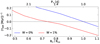 |
Fig. 2. Net torque in units of the stellar AM versus Rt/Rco and P⋆ for two values of the wind parameter W. For the wind scenario, the zero-torque condition (horizontal line) is reached at lower values compared to the no-wind scenario. The stellar parameters are as follows: Ṁ⋆ = 0.7 M⊙, B⋆ = 0.5 kG, Ṁ⋆ = 3 × 10⁻⁹ M⊙ yr−1, and τage = 2 Myr. |
The equilibrium state for the no-wind scenario with W = 0% and the wind scenario with W = 1% is shown in Fig. 3 over a range of stellar accretion rates typical for T Tauri stars. We considered stellar ages τage of 2 Myr (solid lines) and 5 Myr (dashed lines). For comparison, we show the observed distribution of stellar accretion rates, Ṁobs, at 1–3 and 3–8 Myr from Betti et al. (2023). In the range of Ṁobs, the APSW reduces the equilibrium values of ℛ by 15–35%. The dependence of rA on Rt and Ṁ⋆ results in an increasing efficiency of the APSW with higher accretion rates. Analogous to the no-wind scenario, the equilibrium values remain between 0.433 ≤ ℛ ≤ 1.0 (State 2), indicating that the APSW alone cannot counteract the spin-up torques (e.g., Zanni & Ferreira 2011). The break in the equilibrium values of ℛ for W = 1% can be explained by the transition of Rt close to Rco (see Eq. (1) and Fig. 1) and also depends on B⋆. In contrast, the stellar mass dependence of the equilibrium state is weak compared to the effect of an APSW (see also Fig. 4). The equilibrium state shown in Fig. 3 is based on fixed stellar and disk parameters. However, the parameters do not stay constant but evolve over million years. For example, the stellar radius contracts during pre-main sequence evolution, and the accretion rate decreases during the Class II phase. Thus, the equilibrium value of ℛ slowly changes over time. The star, however, remains close to its equilibrium state during its evolution once the state is reached (e.g., Ireland et al. 2022; Serna et al. 2024).
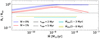 |
Fig. 3. Equilibrium state values of Rt/Rco over stellar accretion rates. We compare the no-wind with the wind scenario for two stellar ages, τage = 2 Myr and τage = 5 Myr. The observed range of stellar accretion rates is shown for stellar ages between 1 Myr and 8 Myr. The stellar mass is 0.7 M⊙, and B⋆ = 0.5 kG. The horizontal dashed lines enclose State 2 (Eq. (2)). In the region of Ṁ⋆ ∼ 10−7 M⊙ yr−1, the condition Rt ≥ R⋆ would be violated, so these values have been excluded. |
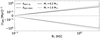 |
Fig. 4. Effect of a short-term deviation from the equilibrium state (as described in Sect. 2.3). The resulting torques that act on the star, in units of the stellar AM, τAM−1, are shown over a range of equilibrium magnetic field strengths. The stellar age is 2 Myr. |
2.3. Effect of short-term variability
Some stellar properties exhibit short-term variability (timescales of τvar≲ years), especially Ṁ⋆ and B⋆. Thus, a star in its equilibrium state is subject to a variation in its parameters and can experience a spin-up or spin-down torque, which introduces scatter in the stellar properties. Typical literature values for these variations are 0.40 dex for Ṁ⋆ (e.g., Manara et al. 2023) and 0.48 dex for B⋆ (e.g., Johnstone et al. 2014; Reiners et al. 2022).
We used this variation to calculate the torque that acts on a star when Ṁ⋆ and B⋆ deviate from their equilibrium values. In Fig. 4, the respective torques are shown over a range of (equilibrium) stellar magnetic field strengths for 2 Myr old stars and W = 0%. Starting from the equilibrium values, we randomly varied Ṁ⋆ and B⋆ within the variation range and calculated the torques on the star while assuming that it still rotates at the equilibrium rate (τvar ≪ τAM). We repeated this process 1000 times, and the solid and dashed lines in the figure mark the 1σ range. Spin-up (spin-down) torques, Δspin up (Δspin down), are marked as solid (dashed) lines. The magnitude of the scatter due to variability, Δspin up and Δspin down, is not significantly changed by the appearance of an APSW. When increasing the stellar age to 5 Myr, the values of Δspin up and Δspin down decreased by a factor of approximately two-thirds due to the smaller stellar radii for older stars and the resulting smaller torques (see Eq. (2) and, e.g., Serna et al. 2024). Since these variations appear to be stochastic, in our simulations we assumed a star may deviate randomly from its equilibrium state within 2Δspin up and 2Δspin down when calculating the spin population model.
2.4. Schematic of the spin population model
The main assumptions of our stellar spin population model (SPM) are as follows. (1) Most stars with ages τage ≳ 1 − 2 Myr have reached their equilibrium state. (2) In their equilibrium state, there is a significant difference in the value of ℛ when comparing the no-wind and wind scenarios (see Fig. 3). (3) Due to the variation in their accretion and magnetic fields, stars can deviate from their equilibrium state within 2Δspin up and 2Δspin down. We generated a population of stars in three steps. First, we selected a stellar mass between 0.2 and 1.0 M⊙ according to the initial mass function of Chabrier et al. (2014). The stellar radius was chosen based on the isochrones of Baraffe et al. (2015) for a selected age. In the second step, the accretion rate was chosen based on the relations presented in Betti et al. (2023), which allow a scatter of two standard deviations. Specifically, for τage = 2 Myr, we used logṀ⋆ = 2.12 × log Ṁ⋆ − 8.11, and for τage = 5 Myr, we used logṀ⋆ = 2.43 × log Ṁ⋆ − 8.21. The 1σ dispersions are 0.76 and 1.06 dex, respectively. In the third step, we randomly chose a magnetic field strength from a uniform distribution between 0.1 and 2.0 kG. For stellar rotation periods between 0.3 and 50 days (the observed range, e.g., Smith et al. 2023), we calculated Rt, Rco, and Γext according to Ireland et al. (2022) and evaluated if 2Δspin down ≤ τAM−1 ≤ 2Δspin up. We note that this assumes that the variability in B⋆ and Ṁ⋆ is uncorrelated. From all periods that fulfill this torque balance condition, we randomly chose the star’s rotation period. We discuss the sensitivity of our results to the choices of these distributions in Appendix A.
Before showing the results of the SPM, we highlight the importance of the parameter ℛ for distinguishing between the no-wind and wind scenarios. The equilibrium state and the torques due to variations in the stellar parameters strongly depend on the magnetic field strength. For a given accretion rate and rotation period, the value ℛ is directly related to B⋆, independent of W (see Eq. (1)). Without a measurement of ℛ, for example, and only measurements of Ṁ⋆ and P⋆, the values of ℛ and B⋆ are degenerate (covariant) and prevent quantitative determinations.
3. Results
We assessed the potential for differentiating between the no-wind and wind scenarios using the distributions of the SPM’s key parameters P⋆, Ṁ⋆, and ℛ. As described in Sect. 2.4, we generated and compared mock distributions of the SPM parameters to estimate the sample size required to achieve a 3σ level of statistical confidence. The mock distributions include expected observational uncertainties, increasing the scatter. Values of Ṁ⋆ are subject to uncertainties of 0.35 dex (e.g., Alcalá et al. 2017; Manara et al. 2023). Stellar rotation periods can be observed with uncertainties of only a few percent (e.g., Smith et al. 2023). Thus, the uncertainty in ℛ depends largely on the uncertainty in Rt, which we take to be 0.2R⋆ (Venuti et al., in prep.; Sect. 4.1).
One way to distinguish between the no-wind and wind scenarios is the offset between the mean values of ℛ for different wind scenarios (see Fig. 5). There is a distinct offset (in the mean values) between populations of stars with APSWs and without them (Fig. 5). The histogram on the right of Fig. 5 shows the distribution of the parameter ℛ. For the no-wind and wind scenarios, the maxima of the distributions are located at ≈0.8 − 0.9 and ≈0.6 − 0.7. Although all equilibrium values of ℛ are located within 0.433 ≤ ℛ ≤ 1.0 (State 2), the effects of short-term variability (Sect. 2.3) are responsible for stars being shifted out of their equilibrium into State 1 or State 3. These stars are either spinning up (if located in State 1) or spinning down (if located in State 3) toward their equilibrium in State 2. To compare the scenarios, we generated a sample of 1000 stars while assuming W = 0% as a reference. Then, for different sample sizes (between 10 and 1000 stars), we generated populations for W = 0% and W = 1% and calculated the offsets between the mean values of ℛ of the respective distributions and the reference sample. We repeated this process 1000 times. The resulting mean values and 3σ ranges of the offsets versus sample size are shown in Panel (a) of Fig. 6 for τage = 2 Myr. To distinguish between the wind and no-wind scenarios at a high confidence (3σ) level, we required a sample size of Ncrit ≥ 255 stars. For older stars (τage = 5 Myr), Ncrit reduces to 218. The smaller scatter due to the variability among older stars (see Sect. 2.3) is responsible for this lower value of Ncrit for older stars.
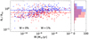 |
Fig. 5. Distribution of the SPM on the |

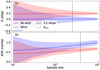 |
Fig. 6. Statistical differentiation between the no-wind and wind scenarios. The offset values of ℛ and the normed value of the overlap of the integrated KDE products are shown in panels a and b. The solid lines are the mean values after 1000 realizations of the SPM. The shaded areas indicate the 3σ range. The stellar age is 2 Myr. |
Alternatively, one can distinguish between the scenarios by comparing the overall parameter distributions, for example, through a kernel density estimator (KDE), which is an estimate of the probability density function. We did not use the Kolmogorov-Smirnov test as its sensitivity decreases toward the tails of the distributions (e.g., Lanzante 2021). To compare two distributions of the SPM parameters P⋆, Ṁ⋆, and ℛ, the respective KDEs are multiplied and the result is integrated over the whole parameter space. The larger the value of this integral, the more the KDEs overlap, and the more similar the distributions are. As a reference and for normalization, we used a population with 1000 stars and assumed W = 0%. Similar to the previous method, this comparison was repeated 1000 times for different sample sizes, assuming W = 0% and W = 1%. The distribution of the metric is shown in Panel (b) of Fig. 6. For this method, we find Ncrit = 395. Similar to the comparison of the offsets, Ncrit decreases to 323 for τage = 5 Myr. The sensitivity of the value of Ncrit on the range of B⋆, short-term variability, and the description of the APSW torque is smaller than ∼30% (Appendix A).
4. Discussion and conclusion
4.1. Availability of observations
Several studies have collected an impressive number of parameters for young stellar objects, including mass, radius, rotation period, and accretion rate (e.g., Betti et al. 2023; Smith et al. 2023). On the other hand, the large-scale magnetic field strength and the location of the truncation radius are poorly constrained by observations. Currently, there are a few dozen observations of magnetic field strengths of accreting stars (e.g., Johnstone et al. 2014; Reiners et al. 2022; Finociety et al. 2023; Flores et al. 2024; Donati et al. 2024a,b) and about as many Rt estimates derived from constraining the size of the Brγ emitting region around young stars with infrared interferometry (Eisner et al. 2014; GRAVITY Collaboration 2023). The ensemble of these observations is not sufficient to adequately test the SPM.
However, the one-dimensional model of time-dependent accretion in young stars developed by Robinson et al. (2021) has enabled the development of the first prescription that directly links light curve morphology and color variability of accreting young stars to the structure of magnetospheric accretion. The theoretical underpinning of this prescription is the following: The kinetic energy of the accretion flow deposited onto the star depends on the distance it traveled from its starting point Rt. This dependence is reflected in the emission spectrum of the resulting accretion shock, which can be probed observationally by measuring the color of the UV excess. A pilot observational program to validate this prescription will be presented in Venuti et al. (in prep.), who employ simultaneous monitoring data of accreting young stars at near-UV and optical wavelengths to populate the stellar loci on color-magnitude diagrams and fit them with the Robinson et al. (2021) grid of predicted color traces to identify the best-fitting magnetospheric parameters. Derived independently of other observational parameters, the value of Rt in combination with Ṁ⋆ and P⋆ can also provide estimates of B⋆ (see Eq. (1)). Thus, the large-scale application of the technique described in Venuti et al. (in prep.) could provide a significant number of Rt and B⋆ measurements and thereby allow valuable insights into stellar spin-down mechanisms.
4.2. Accuracy of the stellar spin model
The main limitation of the SPM lies in the spin model itself. In their study, Ireland et al. (2022) utilize 2.5-dimensional simulations of the star-disk interaction region. Based on these simulations, with runs over several dynamical timescales (≲50 P⋆), relations for the torque acting on the star are extracted (see also Pantolmos et al. 2020) and extrapolated over a large parameter space and the lifetime of PPDs (e.g., Ireland et al. 2021). While producing correct qualitative correlations, the absolute results of the spin model are subject to uncertainties.
Our study demonstrates the sensitivity of the observable ℛ to the presence of an APSW such that with sufficient observations, different stellar spin-down mechanisms (e.g., wind models) can be distinguished. However, we want to highlight certain limitations of our model. One is the predicted stellar rotation period distribution. While the range of observed periods between ∼1 and ∼10 days is reproduced, the peak in the distribution is located at 1–3 days, compared to the observed maximum at 3–4 days (e.g., Smith et al. 2023). The value of the parameter Kt, 1 used in the formulation of the truncation radius Ireland et al. (2022) is smaller by a factor of 0.67 compared to the values in Gallet et al. (2019) and Pantolmos et al. (2020). For a given value of ℛ, the co-rotation radius is smaller by the same amount, and this means faster rotation with periods shorter by a factor of 0.55. This factor could at least partly explain the discrepancy in the rotation period distribution of our SPM compared to observations. Another aspect that varies between spin models is the amount of AM added to the star due to accretion. Magnetic torques and outflows, such as MEs, can remove AM from the disk and at Rt, the disk rotates at velocities smaller than Keplerian (e.g., Gallet et al. 2019). The closer the disk rotates to the Keplerian value, the more AM it carries and the greater the spin-up of the star. Disks rotate at 0.4 and 0.9 times the Keplerian value in the Gallet et al. (2019) and Ireland et al. (2022) models, respectively, thus more AM is transferred onto stars in our SPM.
Our model assumes that the stellar magnetic field is, except for short-term variations, independent of other parameters such as the rotation period. We base this assumption on the small Rossby numbers of T Tauri stars (Ro ≲ 0.1, e.g., Briggs et al. 2007; Johns-Krull 2007). They are usually located in the “saturation” regime of dynamo theory, where the dependence of the magnetic field strength on the rotation period is expected to be weak (B⋆ ∝ P⋆−0.16, e.g., Reiners et al. 2022) and small compared to the short-term variation (cycling) observed in B⋆ (Sect. 2.3).
4.3. Concluding remarks
The relative importance of APSWs compared to, for example, MEs in the spin-down of stars during the T Tauri phase is unclear. The primary purpose of this letter is to describe a method that can evaluate the contribution of APSWs using observations of an appropriate population of Class II young stellar objects. One difference between the spin-down mechanisms manifested itself in the distributions of ℛ = Rt/Rco. Assuming stars during this phase are close to equilibrium (zero-torque state), our SPM predicts a systematic shift in the equilibrium state as an APSW removes AM and reduces ℛ compared to the no-wind case. Monte Carlo simulations using our SPM predict that approximately Ncrit ≳ 250 stars (depending on the age) with simultaneous measurements of truncation radius Rt, rotation period P⋆, and accretion rate Ṁ⋆ are sufficient to differentiate between the no-wind and wind scenarios at a 3σ confidence level.
Our work demonstrates that the value of Ncrit depends on the spin model and statistical evaluation that are used, and its value ranges on the order of several hundred stars. While current observations are inadequate for a test of the spin-down scenario, future uniform surveys of larger samples and application of a spectro-photometric technique to infer Rt from stellar emission alone could prove fruitful.
Acknowledgments
We thank the anonymous referee for constructive feedback that helped to improve the manuscript. EG was supported by NASA Award 80NSSC19K0587 (Astrophysics Data Analysis Program) and NSF Award 2106927 (Astronomy & Astrophysics Research Program) as a Gauss Professor at the University of Göttingen by the Niedersächsische Akaemie der Wissenschaften. NJT acknowledges that this work was carried out in part at the Jet Propulsion Laboratory, California Institute of Technology, under contract 80NM00018D0004 with NASA.
References
- Alcalá, J. M., Manara, C. F., Natta, A., et al. 2017, A&A, 600, A20 [NASA ADS] [CrossRef] [EDP Sciences] [Google Scholar]
- Baraffe, I., Homeier, D., Allard, F., & Chabrier, G. 2015, A&A, 577, A42 [NASA ADS] [CrossRef] [EDP Sciences] [Google Scholar]
- Bessolaz, N., Zanni, C., Ferreira, J., Keppens, R., & Bouvier, J. 2008, A&A, 478, 155 [NASA ADS] [CrossRef] [EDP Sciences] [Google Scholar]
- Betti, S. K., Follette, K. B., Ward-Duong, K., et al. 2023, AJ, 166, 262 [Google Scholar]
- Briggs, K. R., Güdel, M., Telleschi, A., et al. 2007, A&A, 468, 413 [NASA ADS] [CrossRef] [EDP Sciences] [Google Scholar]
- Browning, M. K., Weber, M. A., Chabrier, G., & Massey, A. P. 2016, ApJ, 818, 189 [NASA ADS] [CrossRef] [Google Scholar]
- Chabrier, G., Hennebelle, P., & Charlot, S. 2014, ApJ, 796, 75 [Google Scholar]
- Cody, A. M., & Hillenbrand, L. A. 2010, ApJS, 191, 389 [NASA ADS] [CrossRef] [Google Scholar]
- Donati, J. F., Cristofari, P. I., Alencar, S. H. P., et al. 2024a, MNRAS, 535, 3363 [Google Scholar]
- Donati, J. F., Finociety, B., Cristofari, P. I., et al. 2024b, MNRAS, 530, 264 [NASA ADS] [CrossRef] [Google Scholar]
- Eisner, J. A., Hillenbrand, L. A., & Stone, J. M. 2014, MNRAS, 443, 1916 [Google Scholar]
- Finley, A. J., & Matt, S. P. 2018, ApJ, 854, 78 [Google Scholar]
- Finociety, B., Donati, J. F., Grankin, K., et al. 2023, MNRAS, 520, 3049 [NASA ADS] [CrossRef] [Google Scholar]
- Flores, C., Connelley, M. S., Reipurth, B., Boogert, A., & Doppmann, G. 2024, ApJ, 972, 149 [NASA ADS] [CrossRef] [Google Scholar]
- Gallet, F., & Bouvier, J. 2013, A&A, 556, A36 [NASA ADS] [CrossRef] [EDP Sciences] [Google Scholar]
- Gallet, F., Zanni, C., & Amard, L. 2019, A&A, 632, A6 [NASA ADS] [CrossRef] [EDP Sciences] [Google Scholar]
- GRAVITY Collaboration (Wojtczak, J. A., et al.) 2023, A&A, 669, A59 [Google Scholar]
- Ireland, L. G., Zanni, C., Matt, S. P., & Pantolmos, G. 2021, ApJ, 906, 4 [Google Scholar]
- Ireland, L. G., Matt, S. P., & Zanni, C. 2022, ApJ, 929, 65 [NASA ADS] [CrossRef] [Google Scholar]
- Johns-Krull, C. M. 2007, ApJ, 664, 975 [Google Scholar]
- Johnstone, C. P., Jardine, M., Gregory, S. G., Donati, J. F., & Hussain, G. 2014, MNRAS, 437, 3202 [Google Scholar]
- Koenigl, A. 1991, ApJ, 370, L39 [Google Scholar]
- Lanzante, J. R. 2021, Int. J. Climatol., 41, 6314 [Google Scholar]
- Manara, C. F., Ansdell, M., Rosotti, G. P., et al. 2023, Protostars and Planets VII, ASP Conf. Ser., 534, eds. S.-i. Inutsuka, Y. Aikawa, T. Muto, K. Tomida & M. Tamura (San Francisco: Astronomical Society of the Pacific), 539 [Google Scholar]
- Matt, S., & Pudritz, R. E. 2005, ApJ, 632, L135 [Google Scholar]
- Matt, S., & Pudritz, R. E. 2008, ApJ, 678, 1109 [NASA ADS] [CrossRef] [Google Scholar]
- Matt, S. P., MacGregor, K. B., Pinsonneault, M. H., & Greene, T. P. 2012, ApJ, 754, L26 [Google Scholar]
- Mueller, M. A., Johns-Krull, C. M., Stassun, K. G., & Dixon, D. M. 2024, ApJ, 964, 1 [Google Scholar]
- Pantolmos, G., Zanni, C., & Bouvier, J. 2020, A&A, 643, A129 [NASA ADS] [CrossRef] [EDP Sciences] [Google Scholar]
- Rebull, L. M., Wolff, S. C., Strom, S. E., & Makidon, R. B. 2002, AJ, 124, 546 [Google Scholar]
- Rebull, L. M., Stauffer, J. R., Megeath, S. T., Hora, J. L., & Hartmann, L. 2006, ApJ, 646, 297 [NASA ADS] [CrossRef] [Google Scholar]
- Rebull, L. M., Stauffer, J. R., Cody, A. M., et al. 2020, AJ, 159, 273 [Google Scholar]
- Reiners, A., Shulyak, D., Käpylä, P. J., et al. 2022, A&A, 662, A41 [NASA ADS] [CrossRef] [EDP Sciences] [Google Scholar]
- Réville, V., Brun, A. S., Matt, S. P., Strugarek, A., & Pinto, R. F. 2015, ApJ, 798, 116 [Google Scholar]
- Robinson, C. E., Espaillat, C. C., & Owen, J. E. 2021, ApJ, 908, 16 [NASA ADS] [CrossRef] [Google Scholar]
- Serna, J., Hernandez, J., Kounkel, M., et al. 2021, ApJ, 923, 177 [NASA ADS] [CrossRef] [Google Scholar]
- Serna, J., Pinzón, G., Hernández, J., et al. 2024, ApJ, 968, 68 [NASA ADS] [CrossRef] [Google Scholar]
- Smith, G. D., Gillen, E., Hodgkin, S. T., et al. 2023, MNRAS, 523, 169 [Google Scholar]
- Steiner, D., Gehrig, L., Ratschiner, B., et al. 2021, A&A, 655, A110 [NASA ADS] [CrossRef] [EDP Sciences] [Google Scholar]
- Venuti, L., Bouvier, J., Cody, A. M., et al. 2017, A&A, 599, A23 [NASA ADS] [CrossRef] [EDP Sciences] [Google Scholar]
- Watson, D. M., Calvet, N. P., Fischer, W. J., et al. 2016, ApJ, 828, 52 [NASA ADS] [CrossRef] [Google Scholar]
- Weber, E. J., & Davis, L., Jr 1967, ApJ, 148, 217 [NASA ADS] [CrossRef] [Google Scholar]
- Zanni, C., & Ferreira, J. 2011, ApJ, 727, L22 [NASA ADS] [CrossRef] [Google Scholar]
- Zanni, C., & Ferreira, J. 2013, A&A, 550, A99 [NASA ADS] [CrossRef] [EDP Sciences] [Google Scholar]
Appendix A: Sensitivity tests
In the SPM, we randomly choose the magnetic field strength and the stellar rotation period from the expected variation since the actual distributions of these parameters are poorly constrained. Now, we explore how the results depend on the way these parameters are chosen. First, we change the distribution of B⋆. While the range is still between 0.1 and 2.0 kG, the distribution is centered at 1.5 kG with a deviation of 0.3 kG, shifting the magnetic field strengths to higher values. As a result, the theoretical difference between the wind and no-wind scenarios decreases due to more effective MEs, and the expected variation increases (see Fig. 4). This is reflected by an increase in Ncrit by 30%. Next, we modify the torque variation due to short-term variability (see Sect. 2.3). The torque can still vary between 2Δspin up and 2Δspin down but it is chosen from a normal distribution located at the center of Δspin up and Δspin down with a deviation of the distance between the center Δspin up. As a result, the rotation periods are located closer to the equilibrium state, and the value of Ncrit decreases by 18%.
In this work, we have restricted the wind parameter W to two values, 0% and 1%. It is, however, likely that the values of W are distributed along a certain range. We want to discuss how our results would be affected if W is distributed uniformly between 0% and 2%. Although the variation is mostly unaffected by the value of W (see Sect. 2.3), the equilibrium value of ℛ would change (see Sect. 2.2). For lower values of W, the equilibrium states of the no-wind and wind scenarios are located closer together, resulting in more similar distributions and an increase in Ncrit. Similarly, for higher values of W, Ncrit decreases. As a result, using the aforementioned uniform distribution of W between 0% and 2%, the mean values of the distributions should remain approximately constant while the scatter increases. Thus, Ncrit would also increase but should remain the same order of magnitude. We note that this estimation can change based on the assumed distribution of W.
Finally, we want to discuss the dependence of our results on the APSW model. In this work, we utilize the model presented in Ireland et al. (2022). Compared to other APSW models, for example, the model presented in Matt et al. (2012), which is also used in Gallet et al. (2019), the APSW model of Ireland et al. (2022) includes the effects of an accretion disk leading to stronger dependence of rA on Ṁ⋆. In Appendix B we compare the two wind models in more detail. The average difference between the APSW torque models is relatively small (Fig. B.1) for 10−10 M⊙/yr−1 ≤ Ṁ⋆ ≤ 10−8 M⊙/yr, which is a representative range for the majority of young stars (e.g., Betti et al. 2023). The value of Ncrit increases by ≈20% when using the wind model from Gallet et al. (2019). We note that the parameter ranges used to formulate the APSW models do not completely cover the parameters used in this study (see Appendix C). For specific parameter combinations close to the tails of observed distributions (e.g., very high accretion rates, Ṁ⋆ ∼ 10−7 M⊙ yr−1, and low magnetic field strengths, B⋆ ∼ 0.1 kG), the relations of the stellar spin model are limited. Since the model presented in Ireland et al. (2022) includes the effects of the accretion disk on the Alfvén radius and the average difference compared to other models are small for the majority of observed stars, we have chosen their description to model the APSW torque, knowing that for certain parameter ranges, the relation might be updated in the course of future studies.
Appendix B: Comparison of different APSW models
To assess the impact of specific APSW prescriptions on our results we compare the relative difference between our adopted APSW torque formulation (Ireland et al. 2022) and that adopted by Gallet et al. (2019). In Ireland et al. (2022), the Alfén radius is related to the open magnetic flux of the stellar wind (Réville et al. 2015), yielding the expression of ΓW used in Ireland et al. (2022)
with the fitting parameters KA, 1 = 0.954, KA, 2 = 0.0284, ṀA = 0.394, Kϕ = 1.62, Ṁϕ, 1 = −1.25, Ṁϕ, 2 = 0.184, and the magnetization parameter of the stellar wind
with the total unsigned stellar magnetic flux, Φ⋆ = 2πR⋆2B⋆. In Gallet et al. (2019), the Alfvén radius is calculated according to Matt et al. (2012), yielding
with the values KG1 = 1.7, KG2 = 0.0506, and ṀG = 0.2177.
One important difference between these formulations is the additional dependence of rA on Rt and Ṁ⋆ in Ireland et al. (2022). We show the relative strength of both models in Fig. B.1. At both high and low accretion rates, ΓW could be larger by a factor of roughly two compared to previous models (for the used parameters in Fig. B.1). The presence of an accretion disk affects the dependence of rA on Rt and Ṁ⋆ (e.g., Ireland et al. 2021) and explains the break in ΓW/ΓW, G19. For high accretion rates or low field strengths (with Rt calculated using the first term of Eq. 1), the Alfvén radius scales as  , a much weaker accretion rate dependence than other studies (e.g., Gallet et al. 2019, with
  ) resulting in larger values of rA (possibly exceeding 50R⋆) and ΓW. For low accretion rates (with Rt calculated using the second term of Eq. 1), we find
  resulting in, again, larger values of rA and ΓW compared to Gallet et al. (2019). However, at intermediate accretion rates close to the break in the truncation radius ΓW/ΓW, G19 < 1. Within this formulation of the truncation radius, large values of up to 50R⋆ are possible. Whether such large values of the Alfvén radius are plausible is an open question. While simulations of Pantolmos et al. (2020) and Ireland et al. (2022) occasionally show these values, the parameter ranges used in those studies do not completely overlap with those used in this work, especially high accretion rates at low magnetic field strengths (see Appendix C). In addition, previous studies show significantly smaller values of rA ≲ 20R⋆ (e.g., Matt et al. 2012).
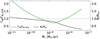 |
Fig. B.1. Comparison of the APSW torque formulation used in this study, ΓW (Eq. B.1), with that in Gallet et al. (2019), ΓW, G19, for a range of accretion rates. In addition, the value of Rt/Rco is shown. The stellar parameters are Ṁ⋆ = 0.7 M⊙, B⋆ = 0.5 kG, P⋆ = 2 days, and τage = 2 Myr. The horizontal line separates the regions in which the respective wind models produce stronger torques. |
To study the sensitivity of our results on the APSW model, we have recalculated the equilibrium values of ℛ using the APSW model from Gallet et al. (2019) (Fig. B.2). For high accretion rates, the values of ℛ are nearly independent of Ṁ⋆ and the difference between the wind models is most pronounced. For the ranges of typical T Tauri accretion rates, however, the models produce similar average results (see also Fig. B.1). At low accretion rates, the equilibrium values are dominated by the effect of MEs, and the strong difference in the wind torques does not significantly affect the values of ℛ.
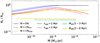 |
Fig. B.2. Same as Fig. 3 but we also use the expression for the APSW torque presented in Gallet et al. (2019) (yellow lines). |
Appendix C: Parameter space in Ireland et al.
For comparison, we compare parameter ranges from the simulations of Ireland et al. (2022) with our parameter space. In Ireland et al. (2022) the accretion rate ranges from 10−11 − 7 × 10⁻⁸ M⊙/yr. The stellar magnetic field strength varies from 0.5 − 2.0 kG and the values of ℛ range from 0.11 to 1.16. The value of W, computed from their parameters as W = Ṁwind/Ṁacc range from 0.3% up to over 100%. The extremely large values of W are obtained for simulation in the propeller regime when the accretion rate sharply drops. The parameter spaces from Ireland et al. (2022) match our parameters for the most part, except for the highest accretion rates of Ṁ⋆ ≈ 10−7 M⊙ yr−1 and the smallest magnetic field strengths of B⋆ < 0.5 kG. Additional simulations would be necessary to explore the full parameter space and possibly find corrections to the given relations.
All Figures
|
Fig. 1. Disk truncation radius Rt in units of stellar radius R⋆ versus accretion rate Ṁ⋆ for a 2 Myr old 0.7-M⊙ star with B⋆ = 0.5 kG and P⋆ = 2 days. The solid line shows the expression given in Eq. (1). The dashed line shows the first term of Eq. (1). The horizontal dashed line marks the co-rotation radius. In the region of Ṁ⋆ ∼ 10−7 M⊙ yr−1, the condition Rt ≥ R⋆ would be violated for the given parameters, so these values have been excluded. |
| In the text | |
|
Fig. 2. Net torque in units of the stellar AM versus Rt/Rco and P⋆ for two values of the wind parameter W. For the wind scenario, the zero-torque condition (horizontal line) is reached at lower values compared to the no-wind scenario. The stellar parameters are as follows: Ṁ⋆ = 0.7 M⊙, B⋆ = 0.5 kG, Ṁ⋆ = 3 × 10⁻⁹ M⊙ yr−1, and τage = 2 Myr. |
| In the text | |
|
Fig. 3. Equilibrium state values of Rt/Rco over stellar accretion rates. We compare the no-wind with the wind scenario for two stellar ages, τage = 2 Myr and τage = 5 Myr. The observed range of stellar accretion rates is shown for stellar ages between 1 Myr and 8 Myr. The stellar mass is 0.7 M⊙, and B⋆ = 0.5 kG. The horizontal dashed lines enclose State 2 (Eq. (2)). In the region of Ṁ⋆ ∼ 10−7 M⊙ yr−1, the condition Rt ≥ R⋆ would be violated, so these values have been excluded. |
| In the text | |
|
Fig. 4. Effect of a short-term deviation from the equilibrium state (as described in Sect. 2.3). The resulting torques that act on the star, in units of the stellar AM, τAM−1, are shown over a range of equilibrium magnetic field strengths. The stellar age is 2 Myr. |
| In the text | |
|
Fig. 5. Distribution of the SPM on the |
| In the text | |
|
Fig. 6. Statistical differentiation between the no-wind and wind scenarios. The offset values of ℛ and the normed value of the overlap of the integrated KDE products are shown in panels a and b. The solid lines are the mean values after 1000 realizations of the SPM. The shaded areas indicate the 3σ range. The stellar age is 2 Myr. |
| In the text | |
|
Fig. B.1. Comparison of the APSW torque formulation used in this study, ΓW (Eq. B.1), with that in Gallet et al. (2019), ΓW, G19, for a range of accretion rates. In addition, the value of Rt/Rco is shown. The stellar parameters are Ṁ⋆ = 0.7 M⊙, B⋆ = 0.5 kG, P⋆ = 2 days, and τage = 2 Myr. The horizontal line separates the regions in which the respective wind models produce stronger torques. |
| In the text | |
|
Fig. B.2. Same as Fig. 3 but we also use the expression for the APSW torque presented in Gallet et al. (2019) (yellow lines). |
| In the text | |
Current usage metrics show cumulative count of Article Views (full-text article views including HTML views, PDF and ePub downloads, according to the available data) and Abstracts Views on Vision4Press platform.
Data correspond to usage on the plateform after 2015. The current usage metrics is available 48-96 hours after online publication and is updated daily on week days.
Initial download of the metrics may take a while.