| Issue |
A&A
Volume 658, February 2022
|
|
|---|---|---|
| Article Number | A102 | |
| Number of page(s) | 11 | |
| Section | Interstellar and circumstellar matter | |
| DOI | https://doi.org/10.1051/0004-6361/202142152 | |
| Published online | 07 February 2022 | |
Unveiling the substructure of the massive clump AGAL G035.1330−00.7450
CONICET - Universidad de Buenos Aires. Instituto de Astronomía y Física del Espacio CC 67,
Suc. 28,
1428
Buenos Aires,
Argentina
e-mail: mortega@iafe.uba.ar
Received:
3
September
2021
Accepted:
26
December
2021
Context. It is known that high-mass stars form as the result of the fragmentation of massive molecular clumps. However, it is not clear whether this fragmentation gives rise to cores that are massive enough to directly form high-mass stars, or if leads to cores of low and intermediate masses that generate high-mass stars by acquiring material from their environment.
Aims. Detailed studies of massive clumps at the early stage of star formation are needed to collect observational evidence that sheds light on the fragmentation processes from clump to core scales. The infrared-quiet massive clump AGAL G035.1330−00.7450 (AGAL35) located at a distance of 2.1 kpc is a promising object for studying the fragmentation and the star formation activity at early stages.
Methods. Using millimeter observations of continuum and molecular lines obtained from the Atacama Large Millimeter Array database at Bands 6 and 7, we studied the substructure of the source AGAL35. The angular resolution of the data at Band 7 is about 0.′′7, which allowed us to resolve structures of about 0.007 pc (~1500 au).
Results. The continuum emission at Bands 6 and 7 shows that AGAL35 harbors four dust cores, labeled C1 to C4, with masses lower than 3 M⊙. Cores C3 and C4 exhibit well-collimated, young, and low-mass molecular outflows related to molecular hydrogen emission-line objects that were previously detected. Cores C1 and C2 present CH3CN J = 13–12 emission, from which we derive rotational temperatures of about 180 and 100 K, respectively. These temperatures allow us to estimate masses of about 1.4 and 0.9 M⊙ for C1 and C2, respectively, which are about an order of magnitude lower than those estimated in previous works and agree with the Jeans mass of this clump. In particular, the moment 1 map of CH3CN emission suggests the presence of a rotating disk towards C1, which is confirmed by the CH3OH and CH3OCHO (20–19) emissions. On the other hand, the CN N = 2–1 emission shows a clumpy and filamentary structure that seems to connect all the cores. These filaments might be tracing the remnant gas of the fragmentation processes taking place within the massive clump AGAL35 or the gas that is being transported toward the cores, which would imply a competitive accretion scenario.
Conclusions. The massive clump AGAL35 harbors four low- to intermediate-mass cores with masses lower than 3 M⊙, which is about an order of magnitude smaller than the masses estimated in previous works. This study shows that in addition to the importance of high-resolution and sensitivity observations for a complete detection of all fragments, it is very important to accurately determine the temperature of these cores for a correct mass estimation. Finally, although no high-mass cores were detected toward AGAL35, the filamentary structure connecting all the cores means that high-mass stars might form through the competitive accretion mechanism.
Key words: stars: formation / ISM: molecules / ISM: jets and outflows
© ESO 2022
1 Introduction
It is known that massive stars (≥8 M⊙) form in clusters that are deeply embedded in massive molecular clumps. Evidence indicates that these clumps, or some of them, can be density-amplified hubs of converging molecular filaments systems, in which according to Kumar et al. (2020), low-mass stars form along the filaments. High-mass stars form in the hubs. These clumps and hubs may collapse under self-gravity and fragment into multiple cores. The number of cores and their mass distribution depends on the processes that regulate the fragmentation. These processes are still a matter of vigorous discussion and debate (Moscadelli et al. 2021; Palau et al. 2018). The mass distribution of the fragments together with the mass reservoir available for the formation of individual stars could give us information for determining whether the massive-starformation is due to an individual monolithic core collapse or to a global hierachical collapse of a clump (Motte et al. 2018). Some years ago, the core-accretion model (McKee & Tan 2002) proposed quasi-equilibrium massive cores that provide all the material for the formation of high-mass stars. In the competitive accretion model (e.g., Bonnell 2008), the parent molecular clump fragments into many low-mass cores that competitively accrete the surrounding gas. It is clear today that the high-mass star formation scenarios are ruled by processes that are not quasi-static, but simultaneously evolve with both cloud and cluster formation (Motte et al. 2018).
The fragmentation of a molecular cloud that leads to different mass distributions of fragments depends on the evolutionarystage of the cloud and on the spatial scale that is considered. As Kainulainen et al. (2013) pointed out, an explanation for the different fragmentation characteristics can be the size-scale-dependent collapse timescale that results from the finite size of real molecular clouds, which is indeed predicted by analytical models (Pon et al. 2011).
Regarding the mass distribution of such molecular fragments, recent studies with spatial resolutions of 0.005–0.02 pc reported a large number of low-mass (≲1 M⊙) molecular fragments in infrared-quiet massive clumps located in high-mass star-forming regions (Palau et al. 2021; Li et al. 2021; Sanhueza et al. 2019). On the other hand, Neupane et al. (2020) and Csengeri et al. (2017b), with similar spatial resolutions, reported limited fragmentation (very few cores and with super-Jeans masses, well above the solar mass) in regions at the early stages of high-mass star formation. Therefore, it is not clear whether the observation of limited fragmentation has a physical origin or is due to an observational issue. For instance, Henshaw et al. (2017), based on high-resolution and high-sensitivity observations, studied a massive clump of about 100 M⊙ located within the infrared dark cloud (IRDC) G035.39−00.33, and found several low- to intermediate-mass cores within a 2–8 M⊙ mass range. The authors concluded that the previously reported dearth of these low-mass objects in this massive clump was due to an observational rather than physical origin, and that some low-mass cores form coevally in the neighborhood of more massive objects. Thus, it is essential to carry out more studies about fragmentation of massive clumps in order to improve the high-mass star formation models.
To better understand the fragmentation and accretion processes that occur at the clump scale, it is crucial to study massive molecular clumps at the earliest stages of star formation with high angular resolution and sensitivity. Thus, we decided to look for some infrared-quiet source with signs of star-forming activity that have interferometric observations. Analyzing the work of Froebrich & Ioannidis (2011), in which several hydrogen emission-line objects (MHOs), which are signs of outflows driven by massive young stellar objects, were detected near the cluster Mercer 14, we realized that some of them coincide with the infrared-quiet massive molecular clump AGAL G035.1330−00.7450 (hereafter AGAL35). According to Csengeri et al. (2017b), this infrared-quiet source presents limited fragmentation, and hence, given that there are related high-angular resolution data in the Atacama Large Millimeter Array (ALMA) database, we concluded that this is a very appropriate source for studying the early massive star-forming processes.
In this work, we present an analysis of the fragmentation and the kinematics of the molecular gas of the massive clump AGAL35 in order to unveil its internal structure. The paper is organized as follows: Sect. 2 presents the source AGAL35, Sect. 3 describes the data, in Sects. 4 and 5 we present results and discussion, respectively, and finally, Sect. 6 states our concluding remarks.
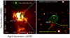 |
Fig. 1 Overview of the H II region G035.126−00.755 at Spitzer-IRAC 8.0 μm image (left). The green contours represent the ATLASGAL emission at 870 μm. Levels are at 0.7, 1.2, 2.6, 4.5, and 7 Jy beam−1. Close-up view of the massive clump AGAL35 at UKIDSS K-band image (right). The green contours represent the ALMA continuum emission at 345 GHz (7 m array from Csengeri et al. 2017b). Levels are at 0.05, 0.10, 0.20, 0.35, and 0.50 Jy beam−1. The beam isindicated in the bottom right corner. The white crosses indicate the position of the two fragments found by Csengeri et al. (2017b) toward AGAL35. The dashed line square indicates the region we studied. |
2 Presentation of the region
The left panel of Fig. 1 shows a Spitzer-IRAC image at 8 μm of the H II region G035.137−00.762. Anderson et al. (2015), based on a radio recombination line, estimated a systemic velocity of 34.5 km s−1 for the H II region, which corresponds to a kinematic distance of about 2.1 kpc. The source AGAL35 appears located in projection toward the bulk of the 8 μm emission. Wienen et al. (2012), based on ammonia (and 13CO) lines, found velocity components at 32 (33) and 35 (36) km s−1 toward AGAL35, with kinetic temperatures of about 20 and 25 K, respectively. Csengeri et al. (2017a) included AGAL35 in a study of an unbiased sample of infrared-quiet massive clumps in the Galaxy that potentially represent the earliest stages of massive cluster formation. They estimated a mass of about 466 M⊙ for this clump.
The right panel of Fig. 1 shows a close-up view of the central region of AGAL35 at the near-infrared K-band obtained from UKIDSS1. The green contours represent the ALMA 7 m continuum emission at 345 GHz presented by Csengeri et al. (2017b). The authors identified two fragments labeled MM1 and MM2, with masses of about 36 and 8 M⊙ (considering a dust temperature of about 25 K), respectively.
Two near-infrared extended sources, labeled ‘Bright’ (A) and ‘Faint EGO’ (B) (Froebrich & Ioannidis 2011) are visible, which are in positional coincidence with the extended green object EGO G035.13−0.74 (hereafter EGO35) cataloged by Cyganowski et al. (2008). The two extended sources are located south of the submillimeter emission.
Finally, Froebrich & Ioannidis (2011) found several molecular hydrogen emission-line objects (MHOs) in the region. Based on GLIMPSE infrared color criteria, they identified possible associated central sources.
3 Data
Data cubes were obtained from the ALMA Science Archive2. We used data from two projects, 2015.1.01312 (PI: Fuller, G.) and 2013.1.00960 (PI: Csengeri, T.), whose observation dates were 2016 March 21 and 2015 April 3, respectively. The observed frequency ranges and the spectral resolutions are 224.24–242.75 GHz and 1.3 MHz (Band 6), and 333.35–348.97 GHz and 1.9 MHz (Band 7) for each project, respectively.
The single-pointing observations for this target were carried out using the following telescope configurations with minimum and maximum baseline(m): 15/460 for project 2015.1.01312, and 15/327.8 for project 2013.1.00960, in the 12 m array in both cases. The maximum recoverable scales at Band 6 and Band 7 are 5.9 and 6.7 arcsec, respectively.
It is important to remark that even though the data of both projects passed the QA2 quality level, which ensures a reliable calibration for science-ready data, the automatic pipeline imaging process may produce a clean image with some artifacts. For example, an inappropriate setting of the parameters of the clean task in CASA could generate artificial dips in the spectra. Thus, we reprocessed the raw data using CASA 4.5.1 and 4.7.2 versions and the calibration pipeline scripts. Particular care was taken with the clean task. The images and spectra obtained from our data reprocessing are very similar to those obtained from the archival images and spectra.
The task imcontsub was used to subtract the continuum from the spectral lines in project 2015.1.01312 using a first-order polynomial. Table 1 presents the main data parameters. The continuum images at 239 and 334 GHz were corrected for primary beam.
Because high spatial resolution is required to perform this study, it is important to remark that the beam size of the 334 GHz data cube provides a spatial resolution of about 0.007 pc (~1500 au) at the distance of 2.1 kpc. This is appropriate for characterizing the substructure of AGAL35.
4 Results
4.1 Continuum emission at 239 and 334 GHz: Tracing the fragmentation of AGAL35
Figure 2 shows the ALMA continuum emission at 334 GHz (12 m array) in grayscale and blue contours. The green contours represent the ALMA continuum emission at 345 GHz (7 m array) presented in the work of Csengeri et al. (2017b). The authors identified two dust condensations related to AGAL35, labeled MM1 and MM2, whose positions are indicated by the green crosses. The better angular resolution of the 334 GHz observations allows us to identify four dust cores toward AGAL35, which are labeled from C1 to C4. The condensation MM1 appears fragmented into cores C1 and C2, while the condensation MM2 seems to be associated with core C4. Two incompletely mapped structures toward the northeast and southeast border of the continuum map are also visible.
Figure 3 shows the continuum emission at 239 GHz extracted from the CH3CN J = 13–12 datacube, where the same four molecular cores can be appreciated. It is important to mention that at 239 GHz, the contamination of the free-free continuum emission might be not negligible. For example, Isequilla et al. (2021) found that toward the core MM1 in the IRDC G34.43+00.24, the contribution of the free-free continuum emission is about 15% at 93 GHz and is negligible at 334 GHz. In AGAL35, while the absence of centimeter radio continuum data prevents us from estimating the free-free emission contribution, the absence of UKIDSS sources associated with the cores (see Sect. 5.2), which indicates the youth of the sources, suggests that the contribution of the ionized gas emission is probably not important toward this region.
Table 2 presents the main parameters of the dust continuum cores observed at 239 and 334 GHz. Columns 2 and 3 give the absolute position, Cols. 4 and 5 present the major and minor axis related to the source size, respectively, from a 2D Gaussian fitting, Cols. 6, 7, and 8 show the peak intensity, the integrated intensity, and the mass, respectively, at 239 GHz, and Cols. 9, 10, and 11 show the same parameters at 334 GHz. Although the core sizes are at least a factor four smaller than the maximum recoverable scales at both frequencies, we cannot discard an underestimation in the calculation of the masses due to the missing flux of the interferometric observations.
The mass of gas for each core was estimated from the dust continuum emission at 239 (λ ~ 1.3 mm) and at 334 GHz (λ ~ 0.9 mm) following Kauffmann et al. (2008),
![\begin{eqnarray*} M_{\textrm{gas}}=0.12~{\textrm{M}_{\odot}} \left[\textrm{exp}\left(\frac{1.439} {(\lambda/\textrm{mm})(T_{\textrm{dust}}/10~\textrm{K})}\right)-1\right],\\ \nonumber \,\,\,\times\left(\frac{\kappa_{\nu}}{0.01~\textrm{cm}^2~\textrm{g}^{-1}}\right)^{-1}\left(\frac{S_{\nu}}\textrm{Jy}\right)\left(\frac{d}{100~\textrm{pc}}\right)^2\left(\frac{\lambda}\textrm{mm}\right)^3\end{eqnarray*}](/articles/aa/full_html/2022/02/aa42152-21/aa42152-21-eq1.png) (1)
(1)
where Tdust is the dust temperature and κν is the dust opacity per gram of matter at 870 μm, for which we adopt the value of 0.0185 cm2 g−1 (Csengeri et al. 2017a, and references therein). Assuming thermal coupling between dust and gas (Tdust = Tkin) and considering a Tkin of about 25 K estimated by Wienen et al. (2012) from the ammonia emission toward AGAL35, we derive masses from 1.3 to 9.4 M⊙ at 239 GHz and from 1.5 to 13.3 M⊙ at 334 GHz (see Table 2).
Main data parameters.
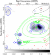 |
Fig. 2 ALMA continuum emission at 334 GHz (12 m array). The color scale unit is Jy beam−1. The blue contour levels are at 15, 30, 50, 80, 140, and 200 mJy beam−1. The green contours correspond to the ALMA continuum emission at 345 GHz (7 m array) reported by Csengeri et al. (2017b). The dashed red contours correspond to −15 mJy beam−1. The beams of both observations are indicated in the top right corner. |
Main dust core parameters at 239 and 334 GHz using a 2D Gaussian fitting from the CASA software.
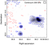 |
Fig. 3 Continuum emission at 239 GHz extracted from the CH3CN J = 13–12 datacube. The grayscale extends from 3 to 45 mJy beam−1. The blue contours levels are at 3, 8, 14, 20, 26, 40, and 65 mJy beam−1. The dashed red contours correspond to −3 mJy beam−1. The beam isindicated in the top right corner. |
4.2 12CO J = 3–2 transition: Molecular outflow activity
Figure 4 shows the integrated velocity channel maps of the 12CO J = 3–2 emission with the continuum emission at 334 GHz superimposed as blue contours. The integration velocity ranges are shown at the top of each panel. The systemic velocity of the complex is about +34.5 km s−1.
The two straight 12CO filaments in panel 1 are shown with magenta and cyan lines and are clearly connected to cores C3 and C4, respectively. Based on the morphology, location, and velocity interval in which these molecular filaments extend, they might correspond to the blue lobes of molecularoutflows arising from each core. The structure labeled B corresponds to molecular gas that is likely related to EGO35, which lies outside the field of view. In panels 2 and 3, the dashed black line shows the direction of a possible rotating disk related to core C1 (see Sects. 4.3 and 4.4). Both panels show molecular gas associated with C1. Panel 3 clearly shows a short filament that appears to be arising from C1 and might indicate molecular outflow activity. Because the direction of this structure is almost the same as the direction of the possible rotating disk (see Sect. 4.3), the hypothesis weakens that it is a molecular outflow. However, although the CH3CN kinematics toward C1 seems to be consistent with a rotating disk, the direction of the outflow candidate might suggest the presence of another embedded source in C1. Therefore the interpretation of the CH3CN spectrum as stemming from multiple velocity components cannot be discarded. Further studies are needed to clarify this. Additionally, panel 2 shows a curved filament that seems to connect cores C2, C3, and C4. Panel 3 shows three molecular features located in projection on the condensation MM1. Finally, panel 4 partially shows two filament-like structures connected to cores C3 and C4, which may be associated with the red lobes of the respective molecular outflows.
The right panel of Fig. 5 displays the 12CO J = 3–2 emission distribution integrated between −18 and +24 km s−1 (in blue) and between + 68 and + 107 km s−1 (in red). The molecular outflows associated with cores C3 and C4 are visible, labeled OC3 and OC4, respectively. The respective red lobes appear to be incomplete. The blue condensation to the south (labeled B) might correspond to the blue lobe of the molecular outflow related to EGO35.
In order to roughly estimate the masses of the blue lobes of the molecular outflows OC3 and OC4 (the red outflows are probably incomplete), we calculated the H2 column density following Bertsch et al. (1993),
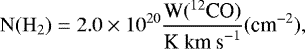 (2)
(2)
where W(12CO) is the 12CO J = 3–2 integrated intensity at the corresponding velocity intervals. The W(12CO) units were converted using
![\begin{equation*} T\,(\textrm{K})=1.22 \times 10^3 \frac{I\,[(\textrm{mJy}\ \textrm{beam}^{-1})]}{\nu^2\,(\textrm{GHz}) ~\theta_{\textrm{maj}}\,(\textrm{arcsec}) \theta_{\textrm{min}}\,(\textrm{arcsec})},\end{equation*}](/articles/aa/full_html/2022/02/aa42152-21/aa42152-21-eq3.png) (3)
(3)
where θmaj and θmin correspond to the major and minor axis of the beam, respectively. Then, the mass of each outflow was derived from
 (4)
(4)
where dΩ is the solid angle subtended by the beam size, mH is the hydrogen mass, μ is the mean molecular weight, assumed to be 2.8 by taking into account a relative helium abundance of 25%, and D is the distance. Ni (H2) is the molecular hydrogen column density (from Eq. (2)) obtained from the 12CO J = 3–2 integrated intensity map (from −18 to +24 km s−1), considering a beam area taken over each blue lobe structure. The summation results from covering the whole extension of each blue lobe (see Fig. 5) with the respective beam area. Table 3 shows the length, the mass, the momentum ( ), and the dynamical age (tdyn = length∕vmax) of each lobe, where
  and vmax are the median and maximum velocities of each interval velocity with respect to the systemic velocity of the gas associated with G35 complex, respectively.
The left panel of Fig. 5 shows the free continuum molecular hydrogen 1–0 S(1) emission line at 2.12 μm extracted from the UWISH2 survey (Froebrich et al. 2011). The perfect alignment of MHO2423 A and B, and the molecular outflow OC4, and of MHO2426 A and B and the molecular outflow OC3 is clear.
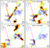 |
Fig. 4 Integrated velocity channel maps of the 12CO J = 3–2 emission. The integration velocity range is exhibited at the top of each panel. The systemic velocity of the gas related to the clump AGAL35 is about 34.5 km s−1. The color scale extends from 0.8 to 16 Jy beam−1 km s−1. Blue contours represent the continuum emission at 334 GHz. Levels are at 15, 30, 50, 80, 140, and 200 mJy beam−1. The magenta and cyan lines indicate the direction of molecular outflow candidates related to the cores C3 and C4, respectively.The dashed black line in panels 2 and 3 indicates the direction of the possible rotating disk related to the core C1. The beam is indicated in the bottom right corner of each map. |
4.3 Analysis of the CH3CN emission: Characterizing cores C1 and C2
CH3CN J = 13–12 emission is observed toward cores C1 and C2. The emission of this symmetric-top molecule is useful to probe temperatures and densities of hot molecular cores and corinos (Remijan et al. 2004).
The center panel of Fig. 6 shows the integrated emission map (K = 0 and K = 1 projections) of the CH3CN J = 13–12 transition. The blue contours represent the ALMA continuum emission at 334 GHz. The position of the CH3CN emission coincides with the location of cores C1 and C2. The left and right panels of Fig. 6 show the average spectra toward cores C1 and C2, respectively. The CH3CN J = 13–12 spectrum toward C1 exhibits conspicuous dip features in all K projections. A possible reason for these dip features might be self-absorption. However, Cesaroni et al. (2014) found an opacity of about 7 associated with the K = 2 projection of the CH3CN J = 12–11 line without dip signatures, therefore this possibility is unlikely. We therefore wonder whether the behavior of the spectrum might correspond to two velocity components associated with a possible rotating disk.
Figure 7 shows the moment 1 map of the CH3CN J = 13–12 emission (K = 3 projection) toward cores C1 and C2. A clear velocity gradient toward core C1 is visible, which has been reported by several works (e.g., Louvet et al. 2016). It might indicate the presence of a rotating disk. The direction of the disk coincides with the direction in which the core C1 exhibits an elongated morphology. Moreover, in the case of rotating disks, symmetric spectral wings are expected, which is particularly evident toward the projections K = 2 and K = 3 of the C1 spectrum (see the right panel of Fig. 6). On the other hand, the behavior of the blended projections K = 0 and K = 1, whose most intense peak presents a higher intensity than the other projections, is better explained as the superposition of the K = 0 blue component and the K = 1 red component than as a consequence of self-absorption effects.
The relevant tabulated numbers for the first five K projections of the CH3CN J = 13–12 transition are presented in Table 4. Columns 1 and 2 show the K projection and the rest frequency, respectively, obtained from NIST catalog3. Column 3 presents the upper energy level (Eu∕k) extracted from the LAMDA database4, and Col. 4shows the line strength of the projection multiplied by the dipole moment of the molecule (Sulμ2).
Table 5 shows the main parameters derived from the Gaussian fittings to the CH3CN spectra of the cores C1 and C2. Columns 2, 3, and 4 show the peak intensity, the Δv, and the integrated intensity (W), respectively. The integrated intensities were used to construct the rotational diagram (RD) presented inFig. 8. Thus, using the RD analysis (Goldsmith & Langer 1999, and references therein) and assuming LTE conditions, optically thin lines, and a beam filling factor equal to the unity, we can estimate the rotational temperature (Trot) and the column density of the CH3CN for cores C1and C2. This analysis is based on a derivation of the Boltzmann equation,
 (5)
(5)
where Nu represents the molecular column density of the upper level of the transition, gu is the total degeneracy of the upper level, Ntot is the total column density of the molecule, Qrot is the rotational partition function, and k is the Boltzmann constant.
Following Miao et al. (1995), for interferometric observations, the left-hand side of Eq. (5) can also be estimated by
 (6)
(6)
where  (in cm−2) is the observed column density of the molecule under the conditions mentioned above, θa and θb (in arcsec) are the major and minor axes of the clean beam, respectively, W (in Jy beam−1 km s−1) is the integrated intensity of each K projection, gk is the K-ladder degeneracy, gl is the degeneracy due to the nuclear spin, ν0 (in GHz) is the rest frequency of the transition, Sul is the line strength of the transition, and μ0 (in Debye) is the permanent dipole moment of the molecule. The free parameters (Ntot∕Qrot) and Trot were determined by a linear fitting of Eq. (5) (see Fig. 8). We derive a Trot of about 190 and 170 K for the blue and red components of core C1, respectively, and of about 100 K for core C2. Using the tabulated value for Qrot at the corresponding temperature, extracted from the CDMS database5, we obtain CH3CN column densities of about 3.1 and 3.3 × 1015 cm−2 for the blue and red components of core C1, respectively, and ~ 1.2 × 1015 cm−2 for core C2.
If optical depths are high, the measured line intensities will not reflect the column densities of the levels. Optical depth effects will be evident in the RD as deviations of the intensities from a straight line and a flattening of the slope, leading to anomalously high values for Trot. The method proposed by Goldsmith & Langer (1999) iteratively corrects individual Nu ∕gu values by multiplying by the optical depth correction factor, Cτ = τ∕(1 −e−τ). However, wefind that the τ corresponding to K = 0 projection isabout 0.002 and 0.003 for cores C1 and C2, respectively, which leads to a correction factor lower than 1%. As expected, the correction factors of the other projections are even smaller.
Finally, considering the integrated intensities at 334 GHz, assuming LTE conditions (Trot = Tkin) with Trot of about 180 and 100 K for cores C1 and C2, respectively, thermal coupling between dust and gas (Tkin = Tdust), and following the same procedure as presented in Sect. 4.1, we re-estimate the masses of cores C1 and C2 to about 1.4 and 0.9 M⊙, respectively.These masses are lower by about an order of magnitude than those calculated using a temperature of 25 K (see Col. 11 in Table 2).
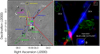 |
Fig. 5 Free continuum molecular hydrogen 1–0 S(1) emission line at 2.12 μm extracted from the UWISH2 survey (left). Green contours represent the ALMA continuum emission at 334 GHz. The red square shows the field of view of the observations presented in this work. The green, blue, and magenta squares, labeled from A to E,indicate the position of the powering source candidates of the MHOs, following Froebrich & Ioannidis (2011). 12CO J = 3–2 emission distribution integrated between −18 and +24 kms−1 (blue) and between +68 and +107 km s−1 (red) (right). Green contours represent the ALMA continuum emission at 334 GHz. The beam is indicated in the top right corner. |
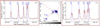 |
Fig. 6 Integrated map of the CH3CN J = 13–12 emission (K = 0, 1 projections) (center). Grayscale unit is Jy beam−1 km s−1. Blue contours represent the continuum emission at 334 GHz. Levels are at 15, 30, 50, 80, 140, and 200 mJy beam−1. The beam is indicated in the top right corner. The spectra of the CH3CN J = 13–12 emission toward C2 and C1 are presented in the left and right panels, respectively. The red curves in both spectra indicate the Gaussian fittings. |
Main parameters of the molecular outflows related to cores C3 and C4.
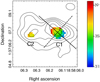 |
Fig. 7 Moment 1 map of the CH3CN J = 13–12 emission (K = 3 projection). The color scale unit is km s−1. The black contours represent the continuum emission at 334 GHz. Levels are at 15, 30, 50, 80, 140, and 200 mJy beam−1. The beam is indicated in the top right corner. The solid and dashed lines show the approximated directions of the disk and its rotation axis, respectively. |
Tabulated parameters for the first five K projections ofCH3CN J = 13–12.
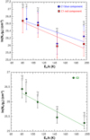 |
Fig. 8 Rotational diagrams of the CH3CN J = 13–12 for the cores C1 (upper panel) and C2 (lower panel). Core C1 is separated into blue and red components. The blue component of the K = 0 projection and the red component of the K = 1 projection are not fit. |
4.4 Tracing the substructure of AGAL35 with other molecules
Figure 9 shows spectra in the frequency ranges 224.68–224.78 GHz and 226.74–226.90 GHz obtained from a region of about 3′′ in radius centered at the position of the condensation MM1. The C17O (2–1), CH3OH (20–19), CH3OCHO (20–19), and CN (2–1) transitions are identified.
Figure 10 shows the integrated emission maps of C17O (2–1), CH3OH 20(−2,19)–19(−3,17)E, CH3OCHO 20(1,19)–19(1,18)(E-A), and CN N = 2–1, J = 5/2–3/2, and F = 7/2–5/2 transitions. The blue contours correspond to the continuum emission at 334 GHz. The integrated emission of CH3OH (20–19) and CH3OCHO (20−19) spatially coincides with the position of cores C1 and C2 at 334 GHz, and no extended emission is detected above the 5σ rms noise level.
On the other hand, the C17O (2–1) integrated map shows extended emission associated with the condensation MM1 (cores C1 and C2). The emission peak appears shifted by about a beam size from the C2 continuum emission peak. A secondary emission peak is located toward the northeastern border of core C1. In addition, the CN (2–1) emission exhibits a clumpy and filamentary structure that seems to connect all the cores. The CN molecular gas shows several condensations whose positions do not coincide with any of the cores. The CN (2–1) emission distribution even seems to surround the core positions, which is particularly evident toward C1.
Figure 11 shows the moment 1 maps for the CH3OH 20(−2,19)–19(−3,17)E and CH3OCHO 20(1,19)–19(1,18) transitions. It shows clear velocity gradients toward core C1 in both molecules, which agrees with what is observed with the CH3CN (13–12) transition. This result reinforces the interpretation of a rotating disk toward C1.
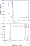 |
Fig. 9 Spectra in the frequency ranges 224.68–224.78 GHz (top) and 226.74–226.90 GHz (bottom) obtained from a region of about 3′′ in radius centered at the position of condensation MM1. |
5 Discussion
5.1 Fragmentation of the massive clump AGAL35
Massive clumps have a relatively low thermal Jeans mass of about 1 M⊙ at typical densities (n ~ 4.6 × 105 cm−3) and temperatures (T ~ 18 K), which predicts a high level of fragmentation. However, Csengeri et al. (2017b), studied a homogeneous sample of infrared-quiet massive clumps (that included AGAL35) and found limited fragmentation from clump to core scales. The average number of fragments was about 3 and the mean mass was about 63 M⊙, which corresponds to massive dense cores (Motte et al. 2007). The authors suggested that early fragmentation of their massive clump sample might not follow thermal processes, showing fragment masses that largely exceeded the local Jeans mass. A possible explanation would be that the selected clumps with the highest peak surface density might correspond to a phase of compactness in which thehigh level of fragmentation required to form a cluster has not yet developed. The authors suggested that a combinationof turbulence, magnetic field, and radiative feedback might have increased the necessary mass for the fragmentation at the early stages.
On the other hand, the authors explored the possibility of a global collapse occurring at cloud scale, in which the equilibrium is not reached on small scales, which could lead to the observed limited fragmentation. When densities of about 102 cm−3 are reached at cloud scales, the initial thermal Jeans mass could reach 50 M⊙, which is still not enough to explain the mass reservoir of the most massive cores of the sample. The authors also suggested that the mass might be replenished beyond the clump scale, which might fuel the formation of the lower-mass population of stars, leading to an increase in the number of fragments with time and allowing a Jeans-like fragmentation to develop at more evolved stages.
Csengeri et al. (2017b) used the ALMA 7 m array at Band 7 with an angular resolution of about 4′′ and identified two cores MM1 and MM2, with masses of 36 and 8 M⊙, respectively, toward AGAL35. This means a total mass of fragments of 44 M⊙. The higher angular resolution and sensitivity of the ALMA data presented in this work allows us to identify four cores embedded within this massive clump. In particular, cores C1 and C2 correspond to the fragmentation of MM1, and cores C3 and C4 would correspond to the fragmentation of MM2. When we assume a temperature of 25 K, the same as in Csengeri et al. (2017b), the total mass in fragments considering the four cores is about 25.7 M⊙ (~60% of the MM1 + MM2 mass) at 334 GHz and about 19.3 M⊙ (~45% of the MM1 + MM2 mass) at 239 GHz. The discrepancy of about a factor 2 between the total mass estimated in this work and those derived by Csengeri et al. (2017b) might be due to the more extended array configuration of our data, based on which part of the envelope emission is not included in the mass estimation.
In the CH3CN J = 13–12 emission, we find temperatures of about 180 and 100 K toward cores C1 and C2, respectively. Moreover, the detection of the CH3OH 20(−2,19)–19(−3,17)E line, with an energy Eu = 514 K, reinforces the temperature above 100 K as estimated from the CH3CN emission. For instance, Ginsburg et al. (2017) used several CH3OH lines with frequencies and Eu close to that presented here and obtained T > 100 K in the W51 high-mass star-forming complex. Therefore, considering these temperatures, the summed mass of cores C1 and C2 of about 2.3 M⊙ (see Sect. 4.3) is lower by about an order of magnitude than the mass reported by Csengeri et al. (2017b) toward core MM1. Considering the parameters of the clump AGAL35 derived in previous works, a temperature of 25 K, a mass of 466 M⊙, and a clump radius of 0.2 pc, we derive a Jeans mass, M_J, and a Jeans length, λJ, of about 0.9 M⊙ and 0.02 pc, respectively. Thus, the masses of the four cores that extend from 0.9 to 3.1 M⊙ and their average separation, which is about 0.04 pc, agree with the expected Jeans mass and length for this clump.
Our results suggest that the fragmentation of the massive clump AGAL35 gave rise to four low-to intermediate-mass cores, and that the main source of discrepancy in the masses estimation is the temperature of the cores. This study shows that in addition to the importance of carrying out high-resolution and high-sensitivity observations in order to have a complete detection of all fragments in a clump, it is very important to accurately determine the temperature of these cores for a correct estimation of their masses.
On the other hand, because our results suggest that the fragmentation of AGAL35 leads to low- to intermediate-mass cores, the only possibility for high-mass star formation to take place in AGAL35 would be the competitive accretion scenario, in which the cores would increase their mass through material flowing through filaments. Observational studies of the kinematics of the molecular gas in star-forming regions (e.g., Schwörer et al. 2019) have found the presence of velocity gradients in hub-filament systems on scales of 0.1 pc, which might indicate mass transport at small scales. In Sect. 5.3 we briefly discuss this possibility.
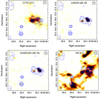 |
Fig. 10 Integrated emission maps of C17O (2–1), CH3OH 20(-2,19)–19(−3,17)E, CH3OCHO 20(1,19)–19(1,18), and CN N = 2–1, J = 5/2–3/2, and F = 7/2–5/2 transitions. The color scale extends from 0.05 to 0.4 Jy beam−1 km s−1 in all panels. Blue contours represent the continuum emission at 334 GHz. Levels are at 15, 30, 50, 80, 140, and 200 mJy beam−1. The beam isindicated in the top right corner of each panel. |
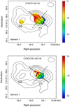 |
Fig. 11 Moment 1 maps of the CH3OH 20(−2,19)–19(−3,17)E and CH3OCHO 20(1,19)–19(1,18) transitions. The color scale unit is km s−1. Black contours represent the continuum emission at 334 GHz. Levels are at 15, 30, 50, 80, 140, and 200 mJy beam−1. The beam isindicated in the top right corner of each panel. The solid and dashed lines show the approximated directions of the disk and its rotation axis, respectively. |
MHOs and their powering source candidates following Froebrich & Ioannidis (2011) (see Fig. 5, left).
5.2 Cores C3 and C4 as powering sources of MHOs
The near-infrared emission from H2 1–0 S(1) lineat 2.122 μm can be generated either by thermal emission in shock fronts or fluorescence excitation by nonionizing UV photons (Martín-Hernández et al. 2008; Frank et al. 2014) that trace the jets or the cavities carved out by the protostar jets and/or winds, respectively. Froebrich & Ioannidis (2011) used UWISH2 data and reported several MHOs toward AGAL35. This shows that the region is an active site of star formation. The authors identified possible sources for some of these MHOs based on infrared color criteria (see Table 6).
We suggest that the infrared-quite cores C3 and C4 are responsible for some MHOs in the region. Figure 5 shows the perfect alignment of the molecular outflow OC4 and MHO2423 A and B, which suggests that the source responsible for these MHOs is core C4. Additionally, the alignment of OC3 and MHO2426 A and B is striking. It indicates that core C3 is responsible for these MHOs. Finally, MHO2424A is likely related to EGO35.
Samal et al. (2018) suggested that H2 emission fades very quickly as the objects evolve from protostars to pre-main-sequence stars, which agrees with the relatively young dynamical age of about 103 yr derived for the molecular outflows related to cores C3 and C4. Moreover, to approximate the evolutionary stage of the sources embedded in the cores C3 and C4, we searched for near-infrared point sources related to these cores in the UKIDSS catalog. The offset between the closest UKIDSS sources and cores C3 and C4 is larger than 1.′′5, which suggests that there is no spatial correlation between the near-infrared sources and these submillimeter cores. The absence of near-infrared emission of the cores indicates that the star formation activity is in its early stages. On the other hand, the well-collimated morphology exhibited by the molecular outflows labeled OC3 and OC4 reinforces the low-mass protostar scenario (Wu et al. 2004).
5.3 Molecules in AGAL35
In this section, we discuss the information that the observed molecular lines give us regarding the cores embedded in the molecular clump AGAL35. Figures 6 and 10 show that the CH3CN, CH3OCHO, and CH3OH are concentrated toward cores C1 and C2, and they do not present extended emission. This fact shows that these molecular species are good tracers of hot molecular cores and corinos, as found in previous works (e.g., Areal et al. 2020; Molet et al. 2019; Beltrán & Rivilla 2018). It is known that these complex molecular species form in the dust grain surfaces, and when the temperature increases, they thermally desorb from the dust. In particular, when the temperature of a molecular core reaches about 90 K, CH3OH thermally desorbs from the grain mantles, and its gas-phase abundance is enhanced close to the protostars (Brown & Bolina 2007).
On the other hand, Fig. 10 shows that the CN (2–1) line traces clumpy extended emission, in agreement with a recent work of Paron et al. (2021), in which the cyano radical emission was analyzed with high-angular resolution ALMA data toward a sample of 10 massive clumps. In particular, toward AGAL35, it is worth noting that the CN peaks do not coincide spatially with the continuum dust cores. Furthermore, it is clear that the CN (2–1) emission seems to surround the cores, which is particularly evident toward C1. This phenomenon was also observed in several other sources (see Paron et al. 2021; Zapata et al. 2008; Beuther et al. 2004). Tassis et al. (2012), based on nonequilibrium chemistry dynamical models, found that the CN molecule is depleted at densities above 105 cm−3. Thus, this molecule apparently does not trace the densest cores, and its emission would arise from the outer layers of very dense gaseous features. On the other hand, a complementary explanation is that the protostars are still deeply embedded in the cores and do not generate enough UV photons to produce CN emission (Beuther et al. 2004). In addition, it is worth mentioning that the missing flux coming from more extended spatial scales that are filtered out by the interferometer could play an important role (Paron et al. 2021).
Interestingly, the CN (2–1) emission toward AGAL35 shows a filamentary structure that seems to connect the four dust cores. These filaments might be tracing the remnant gas from a recent fragmentation that occurred in AGAL35, or they could be mapping the molecular material that is being accreted into the cores. Finally, we discard the notion that the CN filaments can be related to molecular outflows because they do not coincide with the outflow mapped in the 12CO emission or the structures observed at the H2 near-infared emission.
6 Concluding remarks
The massive clump AGAL G035.1330−00.7450 exhibits clear evidence of fragmentation, harboring four low-intermediate mass infrared-quiet cores labeled C1 to C4. Two of them, cores C3 and C4, show well-collimated, young, and low-mass molecular outflows. The main cores C1 and C2 present CH3CN emission from which temperatures of about 180 and 100 K, respectively, are derived. Using these temperatures, we estimate masses of about 1.4 and 0.9 M⊙, which allows us to conclude that these sources are hot corinos. These masses agree with the Jeans mass estimated for this massive clump and are lower by about an order of magnitude than the mass values derived in previous works, in which a clump-scale temperatureof about 25 K was assumed.
This study on the one hand confirms the relevance of high angular resolution and high-sensitivity observations to properly identify the degree of fragmentation of a clump. On the other hand, it reveals the importance of an accurate determination of the core temperatures to estimate their masses. Therefore, it would be interesting to extend this study to a considerable sample of clumps withsimilar characteristics to deeply analyze the phenomenon of limited fragmentation reported by several works.
Interestingly, the CH3CN, CH3OCHO, and CH3OH emission is concentrated toward C1 and C2. In particular, the moment 1 maps obtained from the emission of these three molecules show clear velocity gradients consistent with a rotating disk toward core C1.
Finally, because the masses of all cores in AGAL35 are below 3 M⊙, the only possibility for the formation of high-mass stars would be the competitive accretion mechanism. In this regard, the filamentary structure exhibited by the CN emission might be tracing the gas that falls toward the cores. This would be evidence of a competitive accretion scenario.
Acknowledgements
We thank the anonymous referee for her/his very useful comments. This work was partially supported by grant PICT 2015-1759 awarded by ANPCYT. M.O. and S.P. are members of the Carrera del Investigador Científico of CONICET, Argentina. A.M. and N.I. are doctoral and posdoctoral fellows of CONICET, Argentina. This work is based on the following ALMA data: ADS/JAO.ALMA # 2015.1.01312, and 2013.1.00960. ALMA is a partnership of ESO (representing its member states), NSF (USA) and NINS (Japan), together with NRC (Canada), MOST and ASIAA (Taiwan), and KASI (Republic of Korea), in cooperation with the Republic of Chile. The Joint ALMA Observatory is operated by ESO, AUI/NRAO and NAOJ.
References
- Anderson, L. D., Armentrout, W. P., Johnstone, B. M., et al. 2015, ApJS, 221, 26 [NASA ADS] [CrossRef] [Google Scholar]
- Areal, M. B., Paron, S., Fariña, C., et al. 2020, A&A, 641, A104 [NASA ADS] [CrossRef] [EDP Sciences] [Google Scholar]
- Beltrán, M. T., & Rivilla, V. M. 2018, in Astronomical Society of the Pacific Conference Series, 517, Science with a Next Generation Very Large Array, ed. E. Murphy, 249 [Google Scholar]
- Bertsch, D. L., Dame, T. M., Fichtel, C. E., et al. 1993, ApJ, 416, 587 [Google Scholar]
- Beuther, H., Schilke, P., & Wyrowski, F. 2004, ApJ, 615, 832 [Google Scholar]
- Bonnell, I. A. 2008, in Astronomical Society of the Pacific Conference Series, 390, Pathways Through an Eclectic Universe, eds. J. H. Knapen, T. J. Mahoney, & A. Vazdekis, 26 [Google Scholar]
- Brown, W. A., & Bolina, A. S. 2007, MNRAS, 374, 1006 [NASA ADS] [CrossRef] [Google Scholar]
- Cesaroni, R., Galli, D., Neri, R., & Walmsley, C. M. 2014, A&A, 566, A73 [NASA ADS] [CrossRef] [EDP Sciences] [Google Scholar]
- Csengeri, T., Bontemps, S., Wyrowski, F., et al. 2017a, A&A, 601, A60 [NASA ADS] [CrossRef] [EDP Sciences] [Google Scholar]
- Csengeri, T., Bontemps, S., Wyrowski, F., et al. 2017b, A&A, 600, L10 [NASA ADS] [CrossRef] [EDP Sciences] [Google Scholar]
- Cyganowski, C. J., Whitney, B. A., Holden, E., et al. 2008, AJ, 136, 2391 [Google Scholar]
- Frank, A., Ray, T. P., Cabrit, S., et al. 2014, in Protostars and Planets VI, eds. H. Beuther, R. S. Klessen, C. P. Dullemond, & T. Henning, 451 [Google Scholar]
- Froebrich, D., & Ioannidis, G. 2011, MNRAS, 418, 1375 [CrossRef] [Google Scholar]
- Froebrich, D., Davis, C. J., Ioannidis, G., et al. 2011, MNRAS, 413, 480 [NASA ADS] [CrossRef] [Google Scholar]
- Ginsburg, A., Goddi, C., Kruijssen, J. M. D., et al. 2017, ApJ, 842, 92 [Google Scholar]
- Goldsmith, P. F., & Langer, W. D. 1999, ApJ, 517, 209 [Google Scholar]
- Henshaw, J. D., Jiménez-Serra, I., Longmore, S. N., et al. 2017, MNRAS, 464, L31 [Google Scholar]
- Isequilla, N. L., Ortega, M. E., Areal, M. B., & Paron, S. 2021, A&A, 649, A139 [NASA ADS] [CrossRef] [EDP Sciences] [Google Scholar]
- Kainulainen, J., Ragan, S. E., Henning, T., & Stutz, A. 2013, A&A, 557, A120 [NASA ADS] [CrossRef] [EDP Sciences] [Google Scholar]
- Kauffmann, J., Bertoldi, F., Bourke, T. L., Evans, N. J., I., & Lee, C. W. 2008, A&A, 487, 993 [NASA ADS] [CrossRef] [EDP Sciences] [Google Scholar]
- Kumar, M. S. N., Palmeirim, P., Arzoumanian, D., & Inutsuka, S. I. 2020, A&A, 642, A87 [EDP Sciences] [Google Scholar]
- Li, S., Lu, X., Zhang, Q., et al. 2021, ApJ, 912, L7 [NASA ADS] [CrossRef] [Google Scholar]
- Louvet, F., Dougados, C., Cabrit, S., et al. 2016, A&A, 596, A88 [NASA ADS] [CrossRef] [EDP Sciences] [Google Scholar]
- Martín-Hernández, N. L., Bik, A., Puga, E., Nürnberger, D. E. A., & Bronfman, L. 2008, A&A, 489, 229 [NASA ADS] [CrossRef] [EDP Sciences] [Google Scholar]
- McKee, C. F., & Tan, J. C. 2002, Nature, 416, 59 [CrossRef] [Google Scholar]
- Miao, Y., Mehringer, D. M., Kuan, Y.-J., & Snyder, L. E. 1995, ApJ, 445, L59 [NASA ADS] [CrossRef] [Google Scholar]
- Molet, J., Brouillet, N., Nony, T., et al. 2019, A&A, 626, A132 [EDP Sciences] [Google Scholar]
- Moscadelli, L., Beuther, H., Ahmadi, A., et al. 2021, A&A, 647, A114 [EDP Sciences] [Google Scholar]
- Motte, F., Bontemps, S., Schilke, P., et al. 2007, A&A, 476, 1243 [NASA ADS] [CrossRef] [EDP Sciences] [Google Scholar]
- Motte, F., Bontemps, S., & Louvet, F. 2018, ARA&A, 56, 41 [NASA ADS] [CrossRef] [Google Scholar]
- Neupane, S., Garay, G., Contreras, Y., Guzmán, A. E., & Rodríguez, L. F. 2020, ApJ, 890, 76 [Google Scholar]
- Palau, A., Zapata, L. A., Román-Zúñiga, C. G., et al. 2018, ApJ, 855, 24 [Google Scholar]
- Palau, A., Zhang, Q., Girart, J. M., et al. 2021, ApJ, 912, 159 [NASA ADS] [CrossRef] [Google Scholar]
- Paron, S., Ortega, M. E., Marinelli, A., Areal, M. B., & Martinez, N. C. 2021, A&A, 653, A77 [NASA ADS] [CrossRef] [EDP Sciences] [Google Scholar]
- Pon, A., Johnstone, D., & Heitsch, F. 2011, ApJ, 740, 88 [NASA ADS] [CrossRef] [Google Scholar]
- Remijan, A., Sutton, E. C., Snyder, L. E., et al. 2004, ApJ, 606, 917 [NASA ADS] [CrossRef] [Google Scholar]
- Samal, M. R., Chen, W. P., Takami, M., Jose, J., & Froebrich, D. 2018, MNRAS, 477, 4577 [CrossRef] [Google Scholar]
- Sanhueza, P., Contreras, Y., Wu, B., et al. 2019, ApJ, 886, 102 [Google Scholar]
- Schwörer, A., Sánchez-Monge, Á., Schilke, P., et al. 2019, A&A, 628, A6 [NASA ADS] [CrossRef] [EDP Sciences] [Google Scholar]
- Tassis, K., Willacy, K., Yorke, H. W., & Turner, N. J. 2012, ApJ, 754, 6 [NASA ADS] [CrossRef] [Google Scholar]
- Wienen, M., Wyrowski, F., Schuller, F., et al. 2012, A&A, 544, A146 [NASA ADS] [CrossRef] [EDP Sciences] [Google Scholar]
- Wu, Y., Wei, Y., Zhao, M., et al. 2004, A&A, 426, 503 [NASA ADS] [CrossRef] [EDP Sciences] [Google Scholar]
- Zapata, L. A., Palau, A., Ho, P. T. P., et al. 2008, A&A, 479, L25 [NASA ADS] [CrossRef] [EDP Sciences] [Google Scholar]
All Tables
Main dust core parameters at 239 and 334 GHz using a 2D Gaussian fitting from the CASA software.
MHOs and their powering source candidates following Froebrich & Ioannidis (2011) (see Fig. 5, left).
All Figures
|
Fig. 1 Overview of the H II region G035.126−00.755 at Spitzer-IRAC 8.0 μm image (left). The green contours represent the ATLASGAL emission at 870 μm. Levels are at 0.7, 1.2, 2.6, 4.5, and 7 Jy beam−1. Close-up view of the massive clump AGAL35 at UKIDSS K-band image (right). The green contours represent the ALMA continuum emission at 345 GHz (7 m array from Csengeri et al. 2017b). Levels are at 0.05, 0.10, 0.20, 0.35, and 0.50 Jy beam−1. The beam isindicated in the bottom right corner. The white crosses indicate the position of the two fragments found by Csengeri et al. (2017b) toward AGAL35. The dashed line square indicates the region we studied. |
| In the text | |
|
Fig. 2 ALMA continuum emission at 334 GHz (12 m array). The color scale unit is Jy beam−1. The blue contour levels are at 15, 30, 50, 80, 140, and 200 mJy beam−1. The green contours correspond to the ALMA continuum emission at 345 GHz (7 m array) reported by Csengeri et al. (2017b). The dashed red contours correspond to −15 mJy beam−1. The beams of both observations are indicated in the top right corner. |
| In the text | |
|
Fig. 3 Continuum emission at 239 GHz extracted from the CH3CN J = 13–12 datacube. The grayscale extends from 3 to 45 mJy beam−1. The blue contours levels are at 3, 8, 14, 20, 26, 40, and 65 mJy beam−1. The dashed red contours correspond to −3 mJy beam−1. The beam isindicated in the top right corner. |
| In the text | |
|
Fig. 4 Integrated velocity channel maps of the 12CO J = 3–2 emission. The integration velocity range is exhibited at the top of each panel. The systemic velocity of the gas related to the clump AGAL35 is about 34.5 km s−1. The color scale extends from 0.8 to 16 Jy beam−1 km s−1. Blue contours represent the continuum emission at 334 GHz. Levels are at 15, 30, 50, 80, 140, and 200 mJy beam−1. The magenta and cyan lines indicate the direction of molecular outflow candidates related to the cores C3 and C4, respectively.The dashed black line in panels 2 and 3 indicates the direction of the possible rotating disk related to the core C1. The beam is indicated in the bottom right corner of each map. |
| In the text | |
|
Fig. 5 Free continuum molecular hydrogen 1–0 S(1) emission line at 2.12 μm extracted from the UWISH2 survey (left). Green contours represent the ALMA continuum emission at 334 GHz. The red square shows the field of view of the observations presented in this work. The green, blue, and magenta squares, labeled from A to E,indicate the position of the powering source candidates of the MHOs, following Froebrich & Ioannidis (2011). 12CO J = 3–2 emission distribution integrated between −18 and +24 kms−1 (blue) and between +68 and +107 km s−1 (red) (right). Green contours represent the ALMA continuum emission at 334 GHz. The beam is indicated in the top right corner. |
| In the text | |
|
Fig. 6 Integrated map of the CH3CN J = 13–12 emission (K = 0, 1 projections) (center). Grayscale unit is Jy beam−1 km s−1. Blue contours represent the continuum emission at 334 GHz. Levels are at 15, 30, 50, 80, 140, and 200 mJy beam−1. The beam is indicated in the top right corner. The spectra of the CH3CN J = 13–12 emission toward C2 and C1 are presented in the left and right panels, respectively. The red curves in both spectra indicate the Gaussian fittings. |
| In the text | |
|
Fig. 7 Moment 1 map of the CH3CN J = 13–12 emission (K = 3 projection). The color scale unit is km s−1. The black contours represent the continuum emission at 334 GHz. Levels are at 15, 30, 50, 80, 140, and 200 mJy beam−1. The beam is indicated in the top right corner. The solid and dashed lines show the approximated directions of the disk and its rotation axis, respectively. |
| In the text | |
|
Fig. 8 Rotational diagrams of the CH3CN J = 13–12 for the cores C1 (upper panel) and C2 (lower panel). Core C1 is separated into blue and red components. The blue component of the K = 0 projection and the red component of the K = 1 projection are not fit. |
| In the text | |
|
Fig. 9 Spectra in the frequency ranges 224.68–224.78 GHz (top) and 226.74–226.90 GHz (bottom) obtained from a region of about 3′′ in radius centered at the position of condensation MM1. |
| In the text | |
|
Fig. 10 Integrated emission maps of C17O (2–1), CH3OH 20(-2,19)–19(−3,17)E, CH3OCHO 20(1,19)–19(1,18), and CN N = 2–1, J = 5/2–3/2, and F = 7/2–5/2 transitions. The color scale extends from 0.05 to 0.4 Jy beam−1 km s−1 in all panels. Blue contours represent the continuum emission at 334 GHz. Levels are at 15, 30, 50, 80, 140, and 200 mJy beam−1. The beam isindicated in the top right corner of each panel. |
| In the text | |
|
Fig. 11 Moment 1 maps of the CH3OH 20(−2,19)–19(−3,17)E and CH3OCHO 20(1,19)–19(1,18) transitions. The color scale unit is km s−1. Black contours represent the continuum emission at 334 GHz. Levels are at 15, 30, 50, 80, 140, and 200 mJy beam−1. The beam isindicated in the top right corner of each panel. The solid and dashed lines show the approximated directions of the disk and its rotation axis, respectively. |
| In the text | |
Current usage metrics show cumulative count of Article Views (full-text article views including HTML views, PDF and ePub downloads, according to the available data) and Abstracts Views on Vision4Press platform.
Data correspond to usage on the plateform after 2015. The current usage metrics is available 48-96 hours after online publication and is updated daily on week days.
Initial download of the metrics may take a while.