| Issue |
A&A
Volume 653, September 2021
|
|
|---|---|---|
| Article Number | A44 | |
| Number of page(s) | 28 | |
| Section | Cosmology (including clusters of galaxies) | |
| DOI | https://doi.org/10.1051/0004-6361/202039404 | |
| Published online | 07 September 2021 | |
Clustering of red and blue galaxies around high-redshift 3C radio sources as seen by the Hubble Space Telescope
1
Astronomisches Institut, Ruhr–Universität Bochum, Universitätsstraße 150, 44801 Bochum, Germany
e-mail: ghaffari@astro.ruhr-uni-bochum.de
2
AURA for the European Space Agency, Space Telescope Science Institute, 3700 San Martin Drive, Baltimore, MD 21218, USA
3
Center for Astrophysical Sciences, Johns Hopkins University, 3400 N. Charles Street, Baltimore, MD 21218, USA
4
Harvard-Smithsonian Center for Astrophysics, 60 Garden St., Cambridge, MA 02138, USA
5
Instituto de Astronomía, Universidad Católica del Norte, Avenida Angamos 0610, Casilla, 1280 Antofagasta, Chile
6
Finnish Centre for Astronomy with the European Southern Observatory, University of Turku, Väisäläntie 20, 21500 Piikkiö, Finland
7
Lowell Observatory, 1400 West Mars Hill Road, Flagstaff, AZ 86001, USA
Received:
11
September
2020
Accepted:
19
June
2021
To properly understand the evolution of high-redshift galaxy clusters, both passive and star-forming galaxies have to be considered. Here we study the clustering environment of 21 radio galaxies and quasars at 1 < z < 2.5 from the third Cambridge catalog (3C). We use optical and near-infrared Hubble Space Telescope images with a 2′ field-of-view, where the filters encompass the rest-frame 4000 Å break. Passive red and star-forming blue galaxies were separated in the color–magnitude diagram using a redshift-dependent cut derived from galaxy evolution models. We find that about 16 of 21 radio sources inhabit a galaxy overdensity on scales of 250 kpc (30″) projected radius. The sample shows a diversity of red and blue overdensities and also sometimes a deficiency of blue galaxies in the center. The following tentative evolutionary trends are seen: extended proto-clusters with only weak overdensities at z > 1.6, red overdensities at 1.2 < z < 1.6, and red overdensities with an increased deficit of central blue galaxies at z < 1.2. Only a few 3C sources show a blue overdensity tracing active star-formation in the cluster centers; this rarity could indicate that the powerful quasar activity may quench star-formation in the vicinity of most radio sources. The derived number of central luminous red galaxies and the radial density profiles are comparable to those found in local clusters, indicating that some 3C clusters are already mass-rich and compact.
Key words: Galaxy: evolution / galaxies: clusters: general / galaxies: high-redshift
© ESO 2021
1. Introduction
Detecting galaxy clusters at high-redshift (z > 1) has proven to be a difficult task. Surveys based on X-ray imaging (Fassbender et al. 2011; Mehrtens et al. 2012; Mantz et al. 2018) or the Sunyaev-Zel’dovich effect (Carlstrom et al. 2011) readily detect clusters at z < 1, but only a few dozen have been found beyond this redshift (e.g., Bleem et al. 2015; Hennig et al. 2017; Barrena et al. 2018, 2020; Khullar et al. 2019; Aguado-Barahona et al. 2019; Huang et al. 2020). This may imply either a low space density of high-z clusters or a lack of substantial intra-cluster gas that can be detected by the above methods.
Studies using density enhancements and the red sequence (RS) method (Gladders & Yee 2000) again identify numerous clusters at z < 1, but only a small number above this redshift (Eisenhardt et al. 2008; Muzzin et al. 2009; Wilson et al. 2009; Papovich et al. 2010; Hildebrandt et al. 2011). This suggests that such clusters may indeed be rare at these redshifts and beyond or they might not be recognized because of their low contrast relative to the surrounding field or a lack of prominent red sequences. An alternative to blind searches for galaxy overdensities is to look near regions where one presumes that dense environments already exist, using tracers such as radio galaxies (RGs) and active galactic nuclei (AGN). These imply the presence of supermassive black holes hosted by large galaxies and, therefore, regions where the average density of the universe is likely to be high (e.g., Miley & De Breuck 2008).
Numerous teams have found galaxy overdensities (ODs) around distant AGN and RGs (e.g., Best 2000; Best et al. 2003; Pentericci et al. 2000; Venemans et al. 2007; Haas et al. 2009; Falder et al. 2010, 2011; Galametz et al. 2012; Wylezalek et al. 2013; Hatch et al. 2014; Kotyla et al. 2016; Ghaffari et al. 2017). A similar strategy, using submillimeter galaxies as distant mass beacons, has found proto-clusters up to z ∼ 5 (Steidel et al. 1998; Capak et al. 2011; Cai et al. 2017; Martinache et al. 2018; Miller et al. 2018, 2020). The studies using RGs as mass beacons revealed that galaxy ODs are found around about 50% of the RGs. Some RGs appear to be surrounded by fairly evolved clusters while others are not. However, local AGNs do not appear to be strongly associated with clusters and groups (e.g., Wethers et al. 2021). The lack of overdensities around some radio galaxies and AGNs might indicate lower mass groups or regions where the collapse of structure is not well advanced.
To properly understand the evolution of high-z galaxy clusters, both passive and star-forming galaxies have to be considered, and this should be done ideally with a complete cluster or proto-cluster sample. One suitable high-z radio sample is the third Cambridge catalog (3C), selected at 178 MHz. There are two versions: a smaller one complete down to 10 Jy (Laing et al. 1983) and a larger one, used here, which is complete to about 7.5 Jy and contains 64 radio galaxies and quasars at 1 < z < 2.5 (Spinrad et al. 1985). This latter sample has been used for two other recent studies. Using optical and near-infrared images from a Hubble Space Telescope (HST) snapshot survey of 22 sources from the 3C sample, Kotyla et al. (2016) (K16) detected overdensities around half of these objects. Ghaffari et al. (2017) (G17) combined Spitzer-IRAC imaging at 3.6 and 4.5 μm of the complete 3C sample with optical data from the PanStarrs1 survey and again found that about 50% of radio sources in the high-z 3C sample lie within overdensities, with colors typical of early-type galaxies, and none were found beyond z = 1.5. Unlike previous studies, G17 did not presume a population of evolved RS galaxies. The G17 IRAC cluster study revealed that the ODs should be measurable with a 2′ field-of-view such as provided by the HST images (Hilbert et al. 2016). This led us to perform a new analysis of the environments of 3C sources at high redshifts based on the radial density profiles within the HST images and separating red and blue galaxies. In comparison to the K16 study, we consider fainter galaxies and use different color and magnitude selection criteria.
This paper is organized as follows. Section 2 describes the observations and data. Section 3 presents our main results, which include color–magnitude diagrams of the galaxies, surface density maps and radial profiles around the 3C sources, statistical analysis of the detected over- and under-densities, a classification scheme for color-based cluster morphologies, and a comparison with local clusters. Section 4 discusses the diversity of red and blue galaxy clustering, and addresses evolutionary trends. Section 5 summarizes the results.
Throughout this work we adopt a standard ΛCDM cosmology with H0 = 70 km s−1 Mpc−1, ΩΛ = 0.73, and Ωm = 0.27 (Spergel et al. 2007). With this cosmology, a projected angular distance of 30″ corresponds within 3 percent to 250 kpc over the entire redshift range 1 < z < 2.5. All magnitudes are AB, where zero mag corresponds to 3631 Jy.
2. Images, source catalogs, and photometry
We use the HST sample of 22 radio sources from the 3C catalog originally imaged by Hilbert et al. (2016) using the F606W and F140W filters. This sample was randomly selected from the full 3C catalog based on visibility in the telescope scheduling. We excluded 3C418 because of its low galactic latitude and severe stellar contamination. The sample is shown in Table 1. K16 extracted a catalog of galaxies from the F140W images using Source Extractor (Bertin & Arnouts 1996) and then derived colors from the F606W images within apertures measured from the segmentation image in F140W. All source photometry was placed on the AB system and corrected for Galactic extinction (Schlafly & Finkbeiner 2011). Stars were removed using Source Extractor’s stellarity parameter.
Sample.
Our study uses a deeper source catalog, created with the Source Extractor tool in the same manner as described by K16. The catalog consists of two samples, one detected in both filters (6371 sources) and one in IR only (2484 sources). The full catalog contains about 450 galaxies per 3C field.
To estimate detection and completeness limits in our dataset, we followed the procedure described by Andreon et al. (2000). In contrast to unresolved stars, galaxies are extended and at a given total magnitude the surface brightness decreases with increasing source size; therefore the source detection actually depends on the detectable surface brightness. For each galaxy we measured the total magnitude from Source Extractor and a central surface brightness within a 5 pixel aperture (equivalent to 0 2 in F606W and 0
 64 in F140W). Figure 1 shows the number N of detected galaxies as a function of central surface brightness μ. We fit a straight line to the log(N) vs. μ plot at high surface brightness; deviations from this relation at about 23.5 mag arcsec−2 in F140W indicate the onset of incompleteness in the initial detection of objects. As Fig. 2 shows, the surface brightness incompleteness means that we start to miss objects at about F140W ∼ 24 mag. The true 100% completeness limit is likely to be about one mag brighter, where the entire galaxy cloud is brighter than the central surface-brightness limit. Figure 3 shows the equivalent to Fig. 1 for galaxies detected in F140W and F606W. Table 2 summarizes our findings. As a final test, we introduced artificial galaxies in our images using the IRAF artdata program (a mixture of half spheroids and half disks) and repeated the detection procedures. The resulting incompleteness fractions are consistent with those shown in Table 2. For comparison, an L* galaxy has F140W ∼ 22 mag at z ∼ 1−1.5 (e.g., Gabasch et al. 2004).
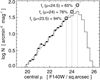 |
Fig. 1. Log(N) versus central surface brightness μ for F140W. The dashed line is a linear fit for 20 < μ < 23.25 (small dots). At μ ≥ 23.5, the histogram declines below the dashed line due to incompleteness. The completeness fractions are calculated as fc = 10data/10fit for three values of μ as labeled and marked with the dotted vertical lines and open circles at the intersection with the dashed line. |
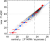 |
Fig. 2. Total F140W magnitude vs. μ. Each galaxy is plotted by a tiny black dot, altogether forming the “galaxy cloud”. The vertical dashed line marks the surface brightness completeness limit at μcl ∼ 23.5. Because the galaxy cloud does not exhibit a sharp boundary at this completeness limit, we proceed as follows: The thick red and blue dots mark the average and standard deviation of μ in the total F140W bins (e.g., 18 < F140W < 19 plotted at F140W = 18.5). The solid blue line is a linear fit through the thick blue dots, which are brighter than μcl. The intersection of the solid blue line with μcl yields a total F140W value ∼24 (horizontal dotted line). At F140W ∼ 24, a large fraction of the galaxy cloud lies right of μcl and therefore suffers from surface brightness incompleteness. The total F140W completeness limit (100%) is likely about 1 mag brighter at 23 mag, where the galaxy cloud is brighter than μcl. |
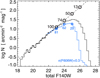 |
Fig. 3. Log(N) versus total F140W magnitude for all galaxies detected in F140W (black histogram). To fit the dashed line, only data points brighter than 22.5 mag were used (small dots). The black numbers indicate the completeness fractions fc = 10data/10fit in percent. The completeness limit fc ∼ 100% lies at 23 mag. To estimate the completeness for objects with colors, the blue histogram shows galaxies detected in both filters. |
Completeness fractions in percent.
3. Analysis and results
We split our sample into four subsets: all (all galaxies, including single band detections), IR-only (galaxies detected in F140W but not in F606W), red and blue where these latter were selected from color-magnitude diagrams as described below.
3.1. Color–magnitude diagrams
Figure 4 shows color-magnitude diagrams for all 21 3C fields. To separate samples of red and blue galaxies, we adopted the RS as identified by K16, based on an evolutionary model from the GALEV tool (Kotulla et al. 2009). Given the relatively large color errors and intrinsic scatter of the RS and uncertainties in the adopted metallicities and formation redshifts, we adopted a color of 1 mag below the RS for galaxies to be defined blue (with the exception of 3C257 where we use a color difference of 0.5 mag as there would otherwise be no “blue” galaxies in this cluster).
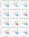 |
Fig. 4. Color–magnitude diagrams (CMDs) for the 3C fields. The labels list the 3C name, type (galaxy or quasar), and redshift. The 3C source is shown as a black diamond if it fits into the plot range (3C 255, 3C 257, 3C 322, 3C 326.1). Red dots and blue stars denote sources in the two-filter catalog, separated by the redshift-dependent color cut (solid black line). The F140W error bars are typically smaller than the size of the symbols but slightly exceed them at the faint end (1σ < 0.3 mag). The color error bars may be larger, reaching 1σ = 0.45 mag, but are not plotted here to avoid confusion. The green symbols mark the sources of the single-filter sample, henceforth denoted the IR-only sample, most of which are fainter than 24 mag. Although their colors are unknown, to illustrate how numerous these sources are they have been randomly assigned colors to fill the upper right quadrant of the CMD. The dashed line marks the 75% color completeness limit, derived from the 3σ detected two-filter sample at F606W = 25 mag and F140W = 23 mag (Table 2) and assuming a slope of −1. |
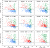 |
Fig. 4. continued. |
Sources detected only in F140W, must be redder than the color selection line shown in Fig. 4. We stacked the F606W images of these objects (based on the positions in F140W) and derived their median color. This is about 0.5 mag redder than objects detected in both filters.
3.2. Surface density: maps and radial profiles
To produce surface density maps, we counted galaxies in circular cells of radius 15″ centered on a 150 × 150 grid with 1″ spacing. Cells falling partially outside of the HST images were masked. We also tried circular cells of radius 10″ and 20″ to test the influence of cell size.
Figure 5 shows surface-density maps and radial density profiles for the 3C 210 field. It is typical for fields with a clear central OD (COD)1. Visual inspection of the maps leaves no doubt that 3C 210 lies in the center of an overdensity of red galaxies with a radial extent of 15″–30″.
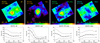 |
Fig. 5. Surface density maps and radial density profiles of the 3C 210 field. Top row: surface density maps for four selection criteria. These are from left to right: all galaxies, red, IR-only and blue galaxies; for red and blue galaxies we used the redshift-dependent color threshold as labeled in the bottom right corner. The magnitude range is 20 < F140W < 26 as labeled in the bottom left corner. The map size is 2.5′, north is up, east to the left. The black cross marks the position of the 3C source. The 3C source is used only as a signpost for a density enhancement and is therefore excluded from the density maps and all further density calculations. The dotted circle indicates the cell size (rc = 15″), and the two solid circles mark a radius of 20″ and 40″ around the 3C source. The color bar at the bottom of the maps gives the linear range used for the map: from N = 0 (black, left end) to the maximal surface density per cell as labeled at the right end of the bar (red); light blue gives the numbers as labeled in the middle of the color bar. Bottom row: mean radial surface density per cell as a function of distance from the 3C source. The radial surface density is plotted for three different cell sizes. The thick line with large dots marks the curve for cell radius rc = 15″, which was used for the maps shown. The two other curves are for rc = 10″ and r = 20″, without area normalization, to avoid confusion of the three curves. |
Beyond r = 30″, essentially no red galaxies are found. In contrast, the blue galaxies avoid the central r = 20″ area and are found in a few clumps at r > 20″. The IR-only galaxies show a clear density enhancement with a peak slightly shifted to the south of 3C 210 but still within 30″ around 3C 210. The IR-only population is about 24–26 mag and may include both blue and red galaxies (Fig. 4), though the stacking results suggest mainly faint red galaxies.
The OD near 3C 210 shows up even when using all galaxies without any color constraints. Maps with cell radius rc = 10″ and rc = 20″ are of sharper and shallower contrasts respectively but are similar to the rc = 15″ maps used for further analysis.
The surface density maps and radial density profiles of the sample for 20 < F140W < 26 are shown in Fig. A.1. The radial density profiles are listed in Table B.1.
Most surface-density maps reveal several density enhancements which, if not caused by fore- or background sources, indicate a clumpy structure of the forming galaxy clusters. The radial surface-density profiles vary among the 3C fields. Both the maps and the profiles depend on the parameters like magnitude and color and slightly on the cell size. Most overdensities have radii r < 30″, and we used the density difference between the area within this radius and that at 30″ < r < 60″ to parameterize the degree of central overdensity (COD). Table 3 summarizes which CODs are significant.
Summary of central over- and under-densities of the 3C clusters, sorted by redshift.
In most cases the 3C source lies within 15″ of the central density enhancement. However, there are few exceptions, for example 3C 297 and 3C 300.1, which both have a red OD shifted toward the south. One could think of shifting the adopted cluster center position, but that position is not unique. 3C 300.1, for instance, exhibits an IR-only COD shifted in a different direction, so that the density enhancements of red and IR-only do not coincide. Therefore, we kept the 3C position as the cluster center.
3.3. Significance and frequency of overdensities
We have calculated the central overdensities as COD = SDC − SDP. The surface density of the center (SDC) and the periphery (SDP) were calculated as the average of the first two and last four data points of the radial density profiles, respectively. The cells entering the SDC calculation reach to r = 14 + 15 = 29″, and the cells entering the SDP calculation reach r = 42−15 = 27″, but the overlap is negligible. Throughout this paper, “periphery” means the outer region surrounding the center as measured on the HST images; it does not imply that the area is beyond the cluster.
To estimate the significance of the COD, a simple approach would be to require that the COD is larger than three times the standard deviation of the periphery σSDP. Unfortunately, this approach fails in most cases, because the subclustering in the periphery increases σSDP. The situation would become even worse, when using external comparison fields, because of the cosmic field-to-field variance. However, for our purpose it is relevant whether there is a local density enhancement centered on the 3C source, irrespective of the presence of other subclustering in the periphery. Therefore, we consider the overdensity as significant, if it is above three times the error of the mean (EoM) of SDP2. Figure 6 illustrates that this approach is reasonable and well justified. Table B.2 lists the surface overdensity for all four catalogs. Figure 7 graphically summarizes the frequency of overdensities; it also shows that the alternative use of the average of the periphery calculated over all 3C sources (vertical dashed and dotted lines) fails in many cases to reveal overdensities because of the large field-to-field variations of the periphery, and therefore for each 3C field its individual periphery is used to quantify the central overdensity relative to the periphery.
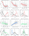 |
Fig. 6. Radial surface density profiles and histograms from the cell counts in Sect. 3.2 for six examples. Top panel: the small “+” symbols mark individual cells, while the colored lines and filled symbols show the mean radial profile and standard deviation. The vertical black dotted and dashed lines mark the radial limits used to define the central region and periphery. Bottom: histogram of the cell counts (made from the “+” in the top row), colored with filled circles for the center and black open circles for the periphery. The vertical lines indicate the average (avg), and for the periphery also the standard deviation (1σ) around the avg and its uncertainty (= error of the mean, |
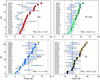 |
Fig. 7. Frequency of central overdensities for the red, IR-only, blue, and all samples for the brightness range 20 < F140W < 26, rc = 15″. In each panel, the 3C sources are sorted by the central surface density (vertical axis). For each 3C source, the horizontal axis shows the surface density of the center (SDC, filled circle) and of the periphery (SDP, horizontal bar with standard deviation as black bar and EoM as thicker blue bar) using values from Table B.2. Crosses within the symbols indicate whether the COD is significant according to approach 1, as described in the text. The vertical lines mark the average of the periphery calculated over all 3C sources (long-dashed line) and the 3σ range (dotted line); the corresponding values are shown in the lower right corner. |
Some 3C sources exhibit a significant COD without any doubt, as confirmed by inspection of the maps (e.g., Fig. 5). Others show no COD. If we use a different range of luminosities, however, the radial profiles of some of these sources indicate a weak COD (Fig. 8). Examples are 3C 68.1, 3C 257, 3C 270.1, 3C 322 3C 326.1, 3C 454.1. In addition to the CODs derived using the standard parameters, Table B.2 lists these fine-tuned cases in the column “comments”.
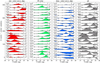 |
Fig. 8. Central overdensities (COD) versus brightness for the red, IR-only, blue and all subsamples. Each row plots the COD around the labeled 3C source, which are sorted by redshift. The rows are subsequently shifted vertically by 20 arcmin−2. The total COD integrated over the brightness range is labeled as Σ. The 3C sources themselves have been excluded from the counts. The brightness bins have a width of 1 mag, which results in small numbers of objects per bin. A COD of N = 5 per square arcmin translates to 1 galaxy per cell of r = 15″. |
About 16 of the 21 observed 3C sources show a significant COD; that means they lie in a clustering of red or IR-only galaxies within a radius of 250 kpc centered on the 3C source. In about 5 of those fields, the red and IR-only COD is accompanied by a blue CUD (negative blue COD), which means that the blue galaxies avoid the center and hence are overdense at radius 250–500 kpc.
Most of the detected CUDs are at z < 1.5 (Table 3). When the blue CUDs are accompanied by a red COD, they are ∼2 mag fainter than the red CODs (e.g., 3C 356, 3C 210). This is consistent with the expectation that the passive (giant) red cluster galaxies are brighter than the star-forming blue galaxies (even at restframe optical wavelengths).
The blue CODs at magnitude 20–23 indicate the presence of luminous star-forming galaxies in the clusters (e.g., 3C 208, 3C 324). Sources with neither blue COD nor CUD are 3C 305.1 and 3C 220.2. At z > 1.5, the detection of blue CODs or CUDs is rare; this could be due to the redshift-dependent blue color cut which leaves few blue galaxies (Fig. 4).
The surface density maps often show several over- and under-densities in the same field (Fig. A.1). Without spectroscopic redshift measurements, we cannot exclude the possibility that some galaxy ODs are at a different redshift, such as a group projected on the line of sight. However, the probability of projected galaxy groups unrelated to a single 3C source is small:
Firstly, the central ODs are fairly well centered on the 3C source (within 15″ radius). They are often accompanied by additional ODs in the surroundings. The red surface density maps show between 1 and 4 ODs per map, on average n1 = 2 ODs. The area of the surface density maps is amap = 2.5 square arcmin. The probability P1 that at least one of the OD centers falls inside r = 15″ around the 3C source is

where a15 is the area inside r = 15″. A red COD is found in 14–15 of the 21 fields. The joint probability of finding 14 or more chance projections is P < 6 × 10⁻⁶. Therefore, chance projections cannot account for the frequency of red CODs.
Secondly, some red CODs are accompanied by blue central underdensities with r > 30″. A pure projection scenario requires that a red OD falls close to the 3C source (P1) and additionally that all (n2) blue clumps lie outside r = 30″ region around the 3C source (P2). The blue surface density maps show between 1 and 6 ODs per map, on average n2 = 4.5 ODs. The probability of n2 out of n2 blue ODs centered in the periphery at r > 30″ is:
![$$ \begin{aligned} P2 = [(a_{\rm map} - a_{30}) / a_{\rm map}]^{n2} = 0.185 = 18.5\%. \end{aligned} $$](/articles/aa/full_html/2021/09/aa39404-20/aa39404-20-eq5.gif)
The combined probability of finding both a red COD and a blue CUD is then Pcomb = P1 * P2 = 0.15 * 0.185 = 0.028 = 2.8%. This estimate is for a single 3C field with red COD and blue CUD. Our sample contains 3 out of 21 such fields. The probability of finding that many (or more) chance projections is P = 0.022 = 2.2%. Again, chance projections make at most a minor contribution to the joint CODs/CUDs.
In addition, the cumulative CODs/CUDs completely disappear when the sky position of the centroid is randomly altered (Sect. 3.5). This rules out a pure projection origin.
3.4. Brightness dependence of the overdensities
Figure 8 shows the CODs versus brightness of the four galaxy types all, red, IR-only and blue. The figure reveals COD brightness trends which depend on the galaxy colors:
-
(1)
red galaxies: at z < 1.3, most 3C sources show a striking COD of red galaxies in the 20−24 magnitude range. At higher redshift (upper half of the panel) the CODs weaken and shift to 21–25 mag. The shift is consistent with the increase of the distance modulus m − M from z = 1 to z = 1.5. This is reminiscent of a wave running through the parameter space, whereby the amplitude decreases with increasing redshift (probably due to incompleteness at faint magnitudes). A few 3C sources lack red CODs in all brightness bins.
-
(2)
IR-only galaxies: nearly all 3C sources show an IR-only COD in at least one magnitude bin, mostly at magnitude 23–26. The IR-only sample contains faint, presumably red galaxies, beyond the completeness limit of the red sample. Therefore the IR-only CODs are likely to be a continuation of the red CODs toward faint magnitudes. 3C sources lacking a red COD but showing a prominent IR-only COD are 3C 186 (z = 1.1), 3C 68.1 (z = 1.2), 3C 298 (z = 1.5), and 3C 454.1 (z = 1.8). These CODs are also supported by the surface density maps; 3C 186 and 3C 454.1 are located between two density enhancements.
-
(3)
blue galaxies: they appear as CODs and UDs (underdensities = negative CODs). The UDs indicate a lack of blue galaxies in the center compared to the periphery. Most UDs are at z < 1.5. When the blue UDs are accompanied by a red COD, they are ∼2 mag fainter than the red CODs (e.g., 3C 356, 3C 210). This is consistent with the expectation that the passive (giant) red cluster galaxies are brighter than the star-forming blue galaxies (even at rest-frame visible wavelengths). On the other hand, the blue CODs at magnitude 20–23, indicate the presence of luminous blue starforming galaxies (e.g., 3C 208, 3C 324). At z > 1.5, the detection of blue CODs or UDs is rare; this could be due to the redshift-dependent blue color cut which leaves few blue galaxies (Fig. 4).
-
(4)
All galaxies: along the entire brightness range, most 3C sources show a clear COD in at least two magnitude bins. For some 3C sources the CODs extend over three to four magnitudes, allowing for an estimate of the luminosity function (LF) of those sources contributing to the CODs.
To summarize, the overdensities show trends with brightness and redshift, albeit with a large spread. At z < 1.5, prominent red CODs are found for galaxies in the 20–23 mag range and these continue to fainter magnitudes (23–26 mag) as IR-only CODs; this may be explained by the incompleteness of our two-filter detections. For blue galaxies, while some CODs are found, the majority of 3C sources exhibit blue underdensities, mostly at faint magnitudes. For the five 3C sources at z > 1.5 (starting with 3C 322), any overdensities are small, and we suggest that this is at least partly due to incompleteness of our shallow imaging.
3.5. Cumulative overdensities
Figure 9 shows the cumulative distribution of overdensities (CCOD) as a function of redshift3. The CCOD slope gives the average COD strength. Most overdensities consist of red galaxies with a relative deficit of blue galaxies close to the 3C source, indicating the presence of a relatively mature cluster population in the inner few hundred kpc.
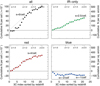 |
Fig. 9. Cumulative central overdensities of the all, red, IR-only and blue samples for the brightness range 20 < F140W < 26 and cell radius rc = 15″. The 3C sources are not included in the counts. The horizontal axis displays the index of each 3C source, sorted by redshift, as labeled at the top of each panel. To guide the eye, the diagonal dotted lines mark slopes of an average central overdensity of s galaxies per cell per 3C field, where the value of s is shown in each panel. |
We estimated the statistical significance of the CCOD in two ways. First, we calculated the cumulative surface densities separately for the central and peripheral regions. A two-sided KS test yields a probability < 10−4 that two distributions drawn from the same population would be so different. (An analogous example is shown in Fig. 10 of G17.) Secondly, we performed a randomized experiment. Instead of the true 3C position, a random position was chosen as the new “center” position and the radial surface density analysis was performed using this location. In all cases this experiment led to a CCOD with constant slope near zero and a noisy curve around this slope; the noise may be due to the fact that the random position is sometimes close to the true 3C position. We repeated this experiment 10 times and averaged the resulting CCODs. Figure 10 shows that the cumulative overdensity disappears in comparison with the corresponding panels in Fig. 9. The marginal negative slope for all and red suggests that for the randomized central positions, the 3C source lies, on average, in the “new” periphery, slightly raising the “new” SDP and lowering the random COD. The randomized results are similar for other brightness bins. The two methods confirm that the CODs and CCODs seen in Fig. 9 are associated with the 3C sources.
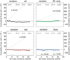 |
Fig. 10. Result of calculating the central overdensities and their cumulative diagrams for randomized positions of the 3C sources. The average counts per cell were determined from 10 random realizations for all four subsamples, as indicated. We note the disappearance of the cumulative overdensity in comparison to Fig. 9. The dotted lines mark slopes as in Fig. 9. |
Figure 11 shows the CCOD for different brightness bins and the samples all, red, IR-only, and blue; the CCODs were calculated using the COD values shown in Fig. 8. The slopes of the brightness-dependent CCODs corroborate the trends seen in Fig. 8. The red overdensities are essentially made up of bright galaxies (21–23 mag) with CCOD slopes (s ∼ 10 galaxies per square arcmin per 3C field) turning-over at z = 1.2 and z = 1.5, respectively. For fainter red galaxies (23–24 mag) the slope flattens (s ∼ 5). The flattening by a factor of about two is stronger than expected from the ∼70% completeness (row 4 of Table 2). The incompleteness of faint red galaxies is further compensated for by the IR-only sample (23–25 mag). The IR-only CCODs show only little turn-over at z > 1.5 and their slopes (s ∼ 5) match the bright red slopes (s ∼ 10) flattened by the completeness fractions (∼50%, row 3 of Table 2). The blue CCODs reveal that the observed deficiency of central blue galaxies is strongest at 23–24 mag and z < 1.2 (s ∼ −5). It is still discernable at fainter magnitudes and larger redshift but these blue galaxies suffer from incompleteness (∼50%, row 6 of Table 2).
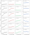 |
Fig. 11. Cumulative central overdensities for different brightness and the samples all, red, IR-only, and blue (from left to right). The 3C sources are excluded from the counts. The horizontal axis is the index of the 3C source, sorted by redshift, as labeled at the top of each panel. The diagonal dotted line marks a slope of a cumulative central overdensity of s = 10 galaxies per square arcmin per 3C field (∼2 galaxies per cell of 15″ radius, for comparison with Fig. 9). For the blue sample, the vertical axis is shifted and zoomed compared to the other three samples. |
To summarize, the brightness-dependent CCODs yield a consistent average picture of bright and faint red overdensities across 3–4 mag as well as blue underdensities. Tentatively correcting the overdensity for incompleteness at faint magnitudes suggests a well-established faint red galaxy population in some but not in all 3C fields (a counter example is 3C 305.1).
3.6. Classification scheme of 3C clusters
The clustering of red and blue galaxies around the 3C sources shows a diversity of over- and under-densities. To bring some order to this jumble, sorting is required as in many fields of astronomy, and for that we used simple mathematical combinatorics. We started by considering all (theoretically) possible combinations, here called classes: red COD, red COD and blue COD, red COD and blue CUD, blue COD, blue COD and red CUD, and so on. We assigned each 3C source to a class, combining the color-dependent COD and CUD results for the red (including IR-only) and blue samples into a joint scheme. This way the environments are sorted by galaxy color and cluster morphology into six classes listed in Table 3. We arranged the six classes in an intuitive way, guided by various scenarios for cluster evolution. In the description of the classes, we assume that the red and blue galaxies are passive and star-forming, respectively. The classes are:
-
(I)
red COD + blue CUD: clusters with a red central overdensity surrounded by a peripheral blue density enhancement. These may be the most evolved clusters in the sample, hosting passive galaxies in the center and star-forming galaxies further out. Our sample contains three certain members of this class, all at z < 1.2, with two additional less certain members.
-
(II)
red COD only: clusters with a red central overdensity but neither an over- nor under-density of blue galaxies. Compared to class I, they do not exhibit a central underdensity of blue galaxies relative to the periphery. Compared to class III, the blue central overdensity has declined to the level of the periphery. Our sample contains eight certain members of this class, all at z < 1.5, plus two less certain members at z > 1.6.
-
(III)
red COD and blue COD: clusters with co-spatial red and blue central overdensities, with star-forming galaxies (still) in the center. The star formation activity may be due to a younger cluster age or to the merger of clusters. Our sample contains two certain members of this class, both at z < 1.3.
-
(IV)
blue COD without red COD: the center hosts a group of star-forming galaxies but not yet on the RS; if these red galaxies do exist, their distribution is extended, indicating a young cluster or proto-cluster. Our sample contains only one member of this class, 3C 432 at z = 1.785: its blue COD is based on a small excess of only 2–3 galaxies. Therefore the classification is uncertain and could change to class VI.
-
(V)
blue CUD only: clusters with no red COD but surrounded by peripheral blue density enhancements. The lack of a red COD suggests that they are evolutionarily young. The powerful radio galaxy may have cannibalized nearby galaxies, but the periphery hosts a reservoir of mostly star-forming galaxies for future cluster (or group) assembly. Our sample contains only two members of this class, both at z < 1.2.
-
(VI)
no COD or CUD at all: any clustering of galaxies is extended on the r = 500 kpc scale, consistent with the expectation for extended proto-clusters. Our sample contains 3–6 members of this class, with 2–5 of them at z > 1.6.
This classification scheme covers all COD/CUD combinations found in our sample. One may think of additional COD/CUD combinations, but they were not seen. Actually, a reduced classification scheme consisting of only two classes would facilitate astrophysical interpretation; two such classes would be quiescent/active clusters lacking/containing star-forming galaxies in their cores.
To be clear: we do not infer the existence of six cluster classes from our small sample of only 21 radio sources; rather the classes are derived from mathematical combinatorics of possible red/blue COD/CUD combinations, and from this we find certain class preferences. This scheme may allow us – using more complete samples in the future – to corroborate evolutionary trends.
Except as noted, the classification at z < 1.6 should be reliable because the CODs/CUDs are well discerned on the surface density maps and the radial density profiles. The CODs/CUDs are based on sufficient galaxies in the red and blue samples (N ≳ 10 with the exception of 3C 305.1).
For z > 1.6, the number of detected galaxies is small. In particular the red sample suffers from severe incompleteness which can not be adequately compensated for by inclusion of the IR-only sample. This makes recognizing CODs/CUDs and the resulting classification uncertain.
3.7. Comparison with local clusters
The number of galaxies in a typical overdensity is < 10 per cell of 15″ radius (Fig. A.1). These overdensities could be galaxy groups or clusters. To check whether the 3C sources are located in massive clusters rather than smaller groups, we compared the richness and spatial concentration of the 3C companions with those of well-studied local clusters. This does not mean that a 3C cluster will evolve into one of the chosen clusters. The local sample comprises 11 Abell clusters from the 2dF cluster survey (De Propris et al. 2003), the Coma cluster (Michard & Andreon 2008), and the Perseus cluster (Meusinger et al. 2020)4.
Most of the Abell clusters are relatively poor, with Abell richness class 0–1, while the Coma and Perseus clusters are more massive systems of richness class 2. The Abell and Coma cluster data cover a radial extent of 1 Mpc, and Perseus is twice of that. The 11 Abell clusters were drawn from the 60 clusters of the 2dF cluster survey, a random collection of clusters from different available catalogs (De Propris et al. 2003) and selected here to have SDSS photometry available. The properties of these comparison clusters are listed in Table 4. All clusters contain spectroscopically confirmed member galaxies with a reported spectroscopic completeness of about 80% (at the bright end about 95%, dropping to 50% at the faint, red end).
Local comparison clusters.
At z ∼ 0, the u and r bands cover a rest-frame part of the spectrum similar to the F606W and F140W filters at 1 < z < 1.5. For the galaxies in Perseus, Meusinger et al. (2020) cataloged u and r band photometry from SDSS. For Coma and the Abell clusters, we obtained u and r from the SDSS DR12 catalog. All photometry was corrected for Galactic foreground extinction (Schlafly & Finkbeiner 2011).
For the local clusters, we selected three galaxy types: bright-red, faint-red, and blue to be compared with the red, IR-only, and blue types of the 3C sources.
In u − r vs. r CMDs, the RS is easily determined by eye, and we applied a color cut u − r = 0.4 below the RS to separate blue and red galaxies. For the 3C sources we had applied a softer color cut F606W − F140W = 1 below the predicted RS, in order to account for the large color uncertainty of both the RS and the faint galaxies in the distant Universe. To separate bright-red and faint-red, we applied a magnitude cut 2.5 mag fainter than the third brightest galaxy in r. This cut was motivated by the transition between red and IR-only CCODs at 23 < F140W < 24, about 2.5 mag fainter than the bright end of the CCODs at F140W = 21 (Fig. 11). Corresponding to the 5 mag brightness range of the galaxies in F140W, for the local clusters we applied a faint end cut of 5 mag fainter than the bright end. For each cluster, we performed the overdensity analysis exactly as done for the 3C sources using a cell radius of 125 kpc (corresponding to 15″ for the 3C sources).
We removed the cD galaxies NGC 1275 (Perseus), NGC 4874, and NGC 4889 (Coma), as we had done for the 3C sources by removing the 3C itself. Figure 13 compares the radial density profiles of fifteen 3C fields at z < 1.5 and the local clusters. The smoothness of the radial profiles shows that the trends are real and significant. Comparison of the 3C sources with the local clusters reveals:
-
(1)
For all four clusters/samples, the bright-red profile declines with increasing radius but with different amplitudes. The central peak of the 3C sources is about N = 90 (per sq. Mpc) above the periphery level at r = 400 kpc. This is a factor 5 larger than the N = 18 peak level of the richness 0–1 Abell clusters. The rich clusters Coma and Perseus have a factor 2–3 higher central peak than the 3C sources.
-
(2)
The profile of the 3C IR-only sources has a peak N = 60 above the periphery level, roughly consistent with the N = 40 peak of the faint-red profile of the Abell clusters. For the Abell clusters, the ratio of faint to bright red galaxies appears constant about 0.5, independent of the radius. As for the bright red galaxies, the rich clusters Coma and Perseus have a 2–3 times higher central peak than the 3C sources. In contrast to the Abell clusters, for Coma the ratio of faint-to-bright red galaxies changes with radius, showing a maximum around r = 250 kpc. This excess of off-center faint-red galaxies in Coma continues to 1 mag fainter galaxies. The radial profile of the very-faint 18 < r < 19 red sources shows that these sources prefer the annulus around 300 kpc and do not peak in the center. This result remains also for Coma’s morphologically identified member galaxies without spectra (Michard & Andreon 2008). For Perseus, faint red galaxies are less numerous than bright ones. This could be due to incompleteness of the faint red population in the spectroscopic sample as noted by Meusinger et al. (2020). Both the 3C’s sources and the spectroscopically confirmed faint red sources of the local clusters suffer from incompleteness (50% for the 3C sources and 10–50% for the local spectroscopic galaxies). To check this, we also plotted the radial profile of all faint red candidate member galaxies. At the central peak (r < 100 kpc) this profile roughly agrees with the spectroscopic profile but then lies a factor 1.5–2 above the spectroscopic profile. Inside r < 500 kpc, it is reminiscent of the IR-only profile of the 3C sources.
-
(3)
The profile of the 3C blue sources exhibits a maximum around r = 400 kpc with a decline toward the center and a small enhancement at r < 100 kpc. The small central enhancement is due to the contribution of the minority of 3C sources with blue COD. The Abell clusters show a similar profile with a dip around r = 250 kpc. The blue profiles of the individual Abell clusters show a large diversity, three/eight with/without blue galaxies in the center. Coma lacks any central blue galaxies (see also Fig. 4 of Andreon 1996). On the other hand, Perseus shows a clear presence of blue galaxies in the center. All local cluster centers show a scarcity of blue galaxies compared to red galaxies.
To summarize, for the 3C sources the radial density profiles of the three galaxy types are quantitatively comparable to those of local clusters. This provides evidence that at least some of the 3C sources are located in clusters and not just in galaxy groups. Other 3C sources may be surrounded by galaxy groups.
4. Discussion and conclusions
The clustering of red and blue galaxies shows a diversity among the 3C sources. The majority are associated with a spatial concentration of red galaxies, most of them with blue galaxies in the periphery, but some 3C sources show also blue galaxies in the center. A few 3C sources lack any COD within 250 kpc. 3C clusters or proto-clusters may be more extended than 250 kpc radius, and therefore the CODs/CUDs we measured mark only the peak of the “cluster iceberg”, and our conclusions will refer to this peak.
4.1. Central overdensity of red and IR-only galaxies
The red and IR-only CODs suggest the presence of a RS. Its bright end has already been shown for seven 3C sources in our sample by K16 using a combination of morphology and colors. The surface density map and overdensity analysis revealed a COD of bright red galaxies in 11/16 (68%) of the 3C sources at z < 1.5. This refers to the roughly L* galaxies of the RS in the central 250 kpc radius. The detection of ∼2 mag fainter RS galaxies is affected by incompleteness of the data, a tentative completeness correction suggests their presence in some but not all 3C fields. The more massive and luminous galaxies are expected to evolve faster than their lower mass counterparts (e.g., Bauer et al. 2005; Conselice et al. 2007). Consequently, the RS may have assembled at the bright end and grown successively toward the faint end. This growth may take place in the center or in the periphery. In our 3C data, the faint RS members have to be searched for in the IR-only data.
Among 3C sources with a clear red COD, some show co-spatial clustering of red and IR-only galaxies, so that both samples show their peak within 20″ around the 3C source (e.g., 3C 210, 3C 230). Some other examples show a strong red COD but a broad spatial distribution of the IR-only galaxies (3C 324, 3C 356).
The observed CODs shift from red to IR-only CODs at z > 1.5, consistent with the increasing distance modulus. A tentative correction of the IR-only CCOD slopes for (about 50%) incompleteness suggests the presence of central overdensities of red galaxies also at z > 1.5, comparable to those at z < 1.5 (Fig. 11). However, visual inspection of the surface density maps (also in narrow magnitude ranges) reveals that any overdensities at z > 1.5 are far more extended than those seen, for instance, for 3C 210 at z < 1.5. This leads us to conclude that red and IR-only overdensities at z > 1.5 are less evolved compared to those at z < 1.5.
4.2. Central lack of blue galaxies, but also blue overdensities
Visual inspection of the surface density maps and radial density profiles reveals a central underdensity (CUD) of blue galaxies for 5/16 of the 3C sources at z < 1.5 (Table 3). Because the central density should not be negative, we conclude that the periphery is overdense in blue galaxies and that these avoid the innermost 250 kpc region around the 3C source. This is most prominent for 3C 186, 3C 210, 3C 287, and 3C 356 (all at z < 1.2), but it is also evident for 3C 305.1.
Three–fourths of the blue CUDs are accompanied by a red or IR-only COD: 3C 186, 3C 210, (3C 305.1 marginal), and 3C 356. These properties imply a spatial segregation of red and blue galaxies in these high-z 3C clusters. One of the blue CUDs appears without corresponding red or IR-only COD: 3C 287, but it lies between two IR-only ODs. These findings from the inspection of the surface density maps and radial density profiles are consistent with the numbers on the radial density profiles in Table B.2. The results for blue CUDs and CODs remain even using a sharper color cut, 0.5 mag below the predicted RS.
On the other hand, two 3C sources, 3C 208 and 3C 324 both at z ≲ 1.2, show a significant blue central overdensity. Their blue COD is accompanied by a pronounced red COD as well. These two clusters contain both passive and star-forming galaxies in their center.
Our 3C sample contains only one source with a blue COD but no red COD; in fact, it is even more extreme because it has a red CUD. If the blue COD and red CUD of 3C 432 at z = 1.8 are both real, then it indicates a clustering of blue galaxies in the center accompanied by a deficit of central red sources. It is unlikely that the powerful radio AGN has cannibalized the red but not the blue galaxies in its vicinity. Therefore, 3C 432 might be located in a compact group of star-forming galaxies, which is part of an extended proto-cluster with 4–6 other subclusters of red and IR-only galaxies (Fig. A.1).
4.3. Evolutionary aspects
We have sorted the diversity of red/blue CODs/CUDs into a classification scheme for the color-dependent cluster morphology (Sect. 3.6, Table 3). This classification scheme was formally guided by simple mathematical combinatorics, but it may reveal possible evolutionary trends of the 3C clusters. Figure 12 plots the cluster class versus redshift.
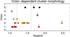 |
Fig. 12. Classification of 3C clusters versus redshift. The vertical axis gives the six classes (I, ..., VI) described in Sect. 3.6. Values are taken from Table 3. A “?” marks uncertain cases. The vertical dotted lines divide the sample at z = 1.2 and z = 1.6. |
The most frequent classes in each redshift group are:
-
Class I at z < 1.2, frequency 4/8, only 2 have class II
-
Class II at 1.2 < z < 1.6, frequency 6/8, none has class I
-
Class VI at z > 1.6, frequency 3/5 but uncertain.
This tentatively suggests two evolutionary trends:
-
(1)
The clusters at z < 1.6 evolve, on average, from class II to class I. The evolution refers to the spatial segregation of central red and peripheral blue galaxies, which becomes more pronounced at lower redshifts5.
-
(2)
For z > 1.6, we see mostly extended proto-clusters. They are likely to evolve to the more concentrated clusters at z < 1.6. This evolutionary trend is consistent with expectations for the proto-cluster/cluster evolution around z ∼ 1.6. However, the classifications are uncertain, as mentioned in Sect. 3.6.
The current sample of 21 clusters is small, and the diversity of cluster types is large. Therefore it is encouraging that consistent evolutionary trends could be derived. The full 3C sample of 64 high-z sources may corroborate these tentative results. The classification scheme is simple and can serve as a useful guide for future studies.
The high-z 3C cluster sample has been selected by using massive radio galaxies as markers for cosmic mass concentrations. How far the classification scheme and the evolutionary trends are applicable to clusters in general needs to be investigated. For instance, powerful AGN activity may quench star-formation in the vicinity of the radio source. On the other hand, Galametz et al. (2009) looked for the frequency of AGN in galaxy clusters at 0 < z < 1.5 selected by X-ray, mid-IR, and radio criteria.
Regardless of selection method, those z > 0.5 clusters show an overdensity of AGNs at r < 500 kpc, and this AGN excess increases with redshift. This suggests that any bias on the cluster properties from using radio galaxies as cluster signposts may be small.
To follow the evolution of the 3C environment to lower redshift (z < 1), homogeneous selection of blue and red galaxies is required for a proper comparison with the high-z results. Regarding X-ray observations, most 3Cs at z < 1 show extended X-ray emission from hot intra-cluster gas, but among the high-z 3C sources only a few have been observed deep enough to allow detection of extended cluster emission (Wilkes et al. 2013; Massaro et al. 2015; Stuardi et al. 2018; Jimenez-Gallardo et al. 2020).
Herschel far-infrared observations of the entire high-z 3C sample have revealed (ultra-)luminous star-forming activity in 22/64 (∼30%) of the 3C sources (Podigachoski et al. 2015). In contrast, the host-normalized SFR of the bulk of the 3C sources at z < 1 is low (Westhues et al. 2016). ULIRG activity suggests major mergers of gas-rich galaxies, and indeed 92% of the high-z 3C sample are associated with recent or ongoing merger events (Chiaberge et al. 2015). Such a merger requires at least one gas-rich (and hence star-forming) galaxy close to the radio source or infalling toward it from the cluster periphery.
If there were many gas-rich companion galaxies in the vicinity of the radio source, they should show up as a blue COD, but this is not observed in the majority of our sample. An explanation could be that the number of gas-rich merger-food galaxies is small. The cannibalization of a single gas-rich galaxy would be sufficient for a major merger which subsequently quenches star-formation in its vicinity.
The richnesses and radial density profiles of the fifteen 3C clusters at 1 < z < 1.5 are, on average, comparable to those of poor local clusters (Fig. 13). About one-third of the 3C sources show red CODs which are a factor 2–3 larger than average, indicating that they are already massive systems (Abell richness class 2 or larger) at these redshifts. If their masses grow further, then their local successors are likely to be very rich clusters (Abell class 3 or larger), which are rare.
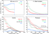 |
Fig. 13. Radial surface density profiles of 3C sources and local clusters for different types of galaxies. The 3C profiles are averaged for red/IR-only/blue galaxies, respectively, using the 15 sources at 1 < z < 1.5 with brightness range 21 < F140W < 26 (top left). For the local clusters, only spectroscopic members are used, split into bright-red, faint-red, and blue. For the 11 Abell clusters, the averaged profiles are shown (top right). The profiles for the Coma and Perseus clusters (bottom) show, in addition, spectroscopically confirmed very faint red sources of Coma and all faint-red candidate cluster members of Perseus; the Perseus samples all bright-red and all blue are not shown because these are spectroscopically 90% complete, so that their profiles remain essentially the same as the profiles of the spectroscopic samples shown. The standard deviations of each radial bin are large and not shown to avoid confusion. |
5. Summary and outlook
We have explored the environment of 21 high redshift 3C sources at 1 < z < 2.5 using HST images in the filters F606W and F140W. These filters encompass the rest frame 4000 Å break. We applied redshift-dependent color cuts to separate passive red and star-forming blue galaxies. The images have a 2′ field-of-view (about 1 Mpc at the 3C’s redshift), yielding about 450 galaxies per 3C environment.
To summarize our methodology and results:
-
The completeness of single-filter-detected galaxies is around 100% at F140W = 23 and 50% at 25 mag. The completeness is lower when F606W detection is also considered. To reduce the incompleteness of faint red galaxies, we include galaxies detected in the F140W filter only. Based on a stacking analysis, the IR-only detected galaxies are about 0.5 mag redder than those detected in two filters.
-
We analysed four galaxy samples: all, red, blue and IR-only. For each sample, surface density maps and radial density profiles show a diversity in the clustering of red and blue galaxies around the 3C sources.
-
At z < 1.5, about 80% of the fields reveal an overdensity of red galaxies within a projected radius r ∼ 250 kpc around the 3C source. The overdensity is defined relative to the mean galaxy density of the periphery (250 kpc, < r < 500 kpc).
-
The probability that fore- and back-ground galaxy groups seen in projection along the line of sight could account for the central overdensity within an individual 3C field is < 15%. Experiments in which the 3C sources were assigned random locations within each image confirm that the likelihood of chance projections is negligible for the sample as a whole. Therefore most of the overdensities are associated with the 3C sources.
-
About three 3C sources show an overdensity of blue galaxies, indicating star-forming activity close to the 3C source.
-
For five 3C sources we found a spatial segregation of red and blue galaxies, with the former populating preferentially the central regions while the latter reside in outer regions of the clusters.
-
The strength and significance of the observed overdensities decrease at z > 1.5. This trend may be due to the lower sensitivity and completeness of our data at these redshifts. Nevertheless, some sources at z < 1.5 lack overdensities, indicating that any clustering has not yet formed the spatial concentration found for most other 3C sources. We suggest that these are proto-clusters in an early assembly phase.
-
At z < 1.5, the overdensities of bright red galaxies could mark the luminous end of the red-sequence. Despite incompleteness of faint red and IR-only galaxies, our data indicate that the red-sequence continues in some but not all 3C sources to about 3 mag fainter than the bright end; in some 3C sources the faint red-sequence galaxies show less spatial concentration than the brighter ones.
-
The diversity of red and blue clustering led us to present a classification scheme of color-dependent cluster morphology. We find a preference of class I and II at z < 1.6 and class VI at z > 1.6, indicating possible different evolutionary states.
-
The derived number of central luminous red galaxies and the radial density profiles are comparable to those found in local clusters, indicating that some 3C clusters are already mass-rich and compact.
With only two filters, the different clustering of red and blue galaxies is efficiently detected, hinting at possible evolutionary trends. These findings are based on a representative subset of the complete 3C sample of 64 high-z sources. The results make future studies with larger fields and larger samples promising, in particular to improve the statistics of the classification scheme, to corroborate the evolutionary trends, and to investigate possible subclustering. While the density maps and the randomized experiments strongly suggest that the density enhancements are associated with the 3C sources, spectroscopic observations will verify cluster membership of the candidates and enable a kinematic study.
EoM =  . SDP has been calculated from N cells. They overlap and thus are not independent. Therefore, we approximated the number of independent cells (Nic) from the areas of periphery (Ap) and cell (Acell): Nic = Ap/Ac. Ap is the area of the HST image (reduced by 15″ for cell radius and 5″ for border) minus the central area of r ∼ 30″. Nic ≈ 13 for Ap = 103 × 116 − π ⋅ 302 square arcsec and rc = 15″.
In order to account for the galaxy ages, the color cuts become bluer with increasing redshift (Fig. 4). Varying the color cuts shows that the absence of blue CUDs at 1.2 < z < 1.6 compared to z < 1.2 is not an observational bias.
Acknowledgments
This work is based on observations taken by the HST-3C collaboration, program GO 13023, with the NASA/ESA HST, which is operated by the Association of Universities for Research in Astronomy, Inc., under NASA contract NAS 5-26555. The 3C environment research at Ruhr-University Bochum is supported by funds from Deutsche Forschungsgemeinschaft (DFG grant HA3555/13-1).
References
- Aguado-Barahona, A., Barrena, R., Streblyanska, A., et al. 2019, A&A, 631, A148 [NASA ADS] [CrossRef] [EDP Sciences] [Google Scholar]
- Andreon, S. 1996, A&A, 314, 763 [NASA ADS] [Google Scholar]
- Andreon, S., Pelló, R., Davoust, E., Domínguez, R., & Poulain, P. 2000, A&AS, 141, 113 [NASA ADS] [CrossRef] [EDP Sciences] [Google Scholar]
- Barrena, R., Streblyanska, A., Ferragamo, A., et al. 2018, A&A, 616, A42 [NASA ADS] [CrossRef] [EDP Sciences] [Google Scholar]
- Barrena, R., Ferragamo, A., Rubiño-Martín, J. A., et al. 2020, A&A, 638, A146 [NASA ADS] [CrossRef] [EDP Sciences] [Google Scholar]
- Bauer, A. E., Drory, N., Hill, G. J., & Feulner, G. 2005, ApJ, 621, L89 [NASA ADS] [CrossRef] [Google Scholar]
- Bertin, E., & Arnouts, S. 1996, A&A, 117, 393 [Google Scholar]
- Best, P. N. 2000, MNRAS, 317, 720 [NASA ADS] [CrossRef] [Google Scholar]
- Best, P. N., Lehnert, M. D., Miley, G. K., & Röttgering, H. J. A. 2003, MNRAS, 343, 1 [NASA ADS] [CrossRef] [Google Scholar]
- Bleem, L. E., Stalder, B., de Haan, T., et al. 2015, ApJS, 216, 27 [NASA ADS] [CrossRef] [Google Scholar]
- Cai, Z., Fan, X., Bian, F., et al. 2017, ApJ, 839, 131 [NASA ADS] [CrossRef] [Google Scholar]
- Capak, P. L., Riechers, D., Scoville, N. Z., et al. 2011, Nature, 470, 233 [Google Scholar]
- Carlstrom, J. E., Ade, P. A. R., Aird, K. A., et al. 2011, PASP, 123, 568 [NASA ADS] [CrossRef] [Google Scholar]
- Chiaberge, M., Gilli, R., Lotz, J. M., & Norman, C. 2015, ApJ, 806, 147 [NASA ADS] [CrossRef] [Google Scholar]
- Conselice, C. J., Bundy, K., Trujillo, I., et al. 2007, MNRAS, 381, 962 [NASA ADS] [CrossRef] [Google Scholar]
- De Propris, R., Colless, M., Driver, S. P., et al. 2003, MNRAS, 342, 725 [NASA ADS] [CrossRef] [Google Scholar]
- Eisenhardt, P. R. M., Brodwin, M., Gonzalez, A. H., et al. 2008, ApJ, 684, 905 [NASA ADS] [CrossRef] [Google Scholar]
- Falder, J. T., Stevens, J. A., Jarvis, M. J., et al. 2010, MNRAS, 405, 347 [NASA ADS] [Google Scholar]
- Falder, J. T., Stevens, J. A., Jarvis, M. J., et al. 2011, ApJ, 735, 123 [NASA ADS] [CrossRef] [Google Scholar]
- Fassbender, R., Nastasi, A., Böhringer, H., et al. 2011, A&A, 527, L10 [NASA ADS] [CrossRef] [EDP Sciences] [Google Scholar]
- Gabasch, A., Bender, R., Seitz, S., et al. 2004, A&A, 421, 41 [NASA ADS] [CrossRef] [EDP Sciences] [Google Scholar]
- Galametz, A., Stern, D., Eisenhardt, P. R. M., et al. 2009, ApJ, 694, 1309 [NASA ADS] [CrossRef] [Google Scholar]
- Galametz, A., Stern, D., De Breuck, C., et al. 2012, ApJ, 749, 169 [NASA ADS] [CrossRef] [Google Scholar]
- Ghaffari, Z., Westhues, C., Haas, M., et al. 2017, Astron. Nachr., 338, 823 [NASA ADS] [CrossRef] [Google Scholar]
- Gladders, M. D., & Yee, H. K. C. 2000, AJ, 120, 2148 [NASA ADS] [CrossRef] [Google Scholar]
- Haas, M., Willner, S. P., Heymann, F., et al. 2009, ApJ, 695, 724 [NASA ADS] [CrossRef] [Google Scholar]
- Hatch, N. A., Wylezalek, D., Kurk, J. D., et al. 2014, MNRAS, 445, 280 [NASA ADS] [CrossRef] [Google Scholar]
- Hennig, C., Mohr, J. J., Zenteno, A., et al. 2017, MNRAS, 467, 4015 [NASA ADS] [Google Scholar]
- Hilbert, B., Chiaberge, M., Kotyla, J. P., et al. 2016, ApJS, 225, 12 [NASA ADS] [CrossRef] [Google Scholar]
- Hildebrandt, H., Muzzin, A., Erben, T., et al. 2011, ApJ, 733, L30 [CrossRef] [Google Scholar]
- Huang, N., Bleem, L. E., Stalder, B., et al. 2020, AJ, 159, 110 [Google Scholar]
- Jimenez-Gallardo, A., Massaro, F., Prieto, M. A., et al. 2020, ApJS, 250, 7 [Google Scholar]
- Khullar, G., Bleem, L. E., Bayliss, M. B., et al. 2019, ApJ, 870, 7 [NASA ADS] [CrossRef] [Google Scholar]
- Kotulla, R., Fritze, U., Weilbacher, P., & Anders, P. 2009, MNRAS, 396, 462 [NASA ADS] [CrossRef] [Google Scholar]
- Kotyla, J. P., Chiaberge, M., Baum, S., et al. 2016, ApJ, 826, 46 [NASA ADS] [CrossRef] [Google Scholar]
- Laing, R. A., Riley, J. M., & Longair, M. S. 1983, MNRAS, 204, 151 [Google Scholar]
- Mantz, A. B., Abdulla, Z., Allen, S. W., et al. 2018, A&A, 620, A2 [NASA ADS] [CrossRef] [EDP Sciences] [Google Scholar]
- Martinache, C., Rettura, A., Dole, H., et al. 2018, A&A, 620, A198 [NASA ADS] [CrossRef] [EDP Sciences] [Google Scholar]
- Massaro, F., Harris, D. E., Liuzzo, E., et al. 2015, ApJS, 220, 5 [NASA ADS] [CrossRef] [Google Scholar]
- Mehrtens, N., Romer, A. K., Hilton, M., et al. 2012, MNRAS, 423, 1024 [NASA ADS] [CrossRef] [Google Scholar]
- Meusinger, H., Rudolf, C., Stecklum, B., et al. 2020, A&A, 640, A30 [NASA ADS] [CrossRef] [EDP Sciences] [Google Scholar]
- Michard, R., & Andreon, S. 2008, A&A, 490, 923 [NASA ADS] [CrossRef] [EDP Sciences] [Google Scholar]
- Miley, G., & De Breuck, C. 2008, A&ARv, 15, 67 [NASA ADS] [CrossRef] [Google Scholar]
- Miller, T. B., Chapman, S. C., Aravena, M., et al. 2018, Nature, 556, 469 [NASA ADS] [CrossRef] [Google Scholar]
- Miller, T. B., Chapman, S. C., Hayward, C. C., et al. 2020, ApJ, 889, 98 [NASA ADS] [CrossRef] [Google Scholar]
- Muzzin, A., Wilson, G., Yee, H. K. C., et al. 2009, ApJ, 698, 1934 [NASA ADS] [CrossRef] [Google Scholar]
- Papovich, C., Momcheva, I., Willmer, C. N. A., et al. 2010, ApJ, 716, 1503 [NASA ADS] [CrossRef] [Google Scholar]
- Pentericci, L., Kurk, J. D., Röttgering, H. J. A., et al. 2000, A&A, 361, L25 [NASA ADS] [Google Scholar]
- Podigachoski, P., Barthel, P. D., Haas, M., et al. 2015, A&A, 575, A80 [NASA ADS] [CrossRef] [EDP Sciences] [Google Scholar]
- Schlafly, E. F., & Finkbeiner, D. P. 2011, ApJ, 737, 103 [NASA ADS] [CrossRef] [Google Scholar]
- Spergel, D. N., Bean, R., Doré, O., et al. 2007, ApJS, 170, 377 [NASA ADS] [CrossRef] [Google Scholar]
- Spinrad, H., Marr, J., Aguilar, L., & Djorgovski, S. 1985, PASP, 97, 932 [NASA ADS] [CrossRef] [Google Scholar]
- Steidel, C. C., Adelberger, K. L., Dickinson, M., et al. 1998, ApJ, 492, 428 [Google Scholar]
- Stuardi, C., Missaglia, V., Massaro, F., et al. 2018, ApJS, 235, 32 [Google Scholar]
- Venemans, B. P., Röttgering, H. J. A., Miley, G. K., et al. 2007, A&A, 461, 823 [NASA ADS] [CrossRef] [EDP Sciences] [Google Scholar]
- Westhues, C., Haas, M., Barthel, P., et al. 2016, AJ, 151, 120 [NASA ADS] [CrossRef] [Google Scholar]
- Wethers, C., Acharya, N., De Propris, R., et al. 2021, IAU Symp., 359, 82 [NASA ADS] [Google Scholar]
- Wilkes, B. J., Kuraszkiewicz, J., Haas, M., et al. 2013, ApJ, 773, 15 [NASA ADS] [CrossRef] [Google Scholar]
- Wilson, G., Muzzin, A., Yee, H. K. C., et al. 2009, ApJ, 698, 1943 [NASA ADS] [CrossRef] [Google Scholar]
- Wylezalek, D., Galametz, A., Stern, D., et al. 2013, ApJ, 769, 79 [NASA ADS] [CrossRef] [Google Scholar]
Appendix A: Surface density: maps and radial profiles of the entire sample
Figure A.1 show the surface density maps and radial profiles of the entire sample. Explanations are given in Sect. 3.2.
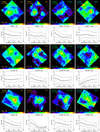 |
Fig. A.1. Surface density maps and radial density profiles of the remaining 3C fields, similar to 3C 210 shown in Fig. 5. |
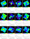 |
Fig. A.1. continued. |
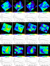 |
Fig. A.1. continued. |
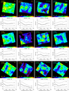 |
Fig. A.1. continued. |
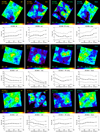 |
Fig. A.1. continued. |
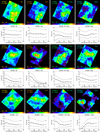 |
Fig. A.1. continued. |
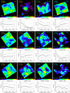 |
Fig. A.1. continued. |
Appendix B: Tables
Radial surface density profiles, as shown in Fig. A.1, using 20 < F140W < 26, cell radius 15″, and radial bins of 7″.
Average surface densities for center and periphery and resulting overdensities in units of N galaxies per cell, using 20 < F140W < 26, cell radius 15″, and radial bins of 7″.
All Tables
Summary of central over- and under-densities of the 3C clusters, sorted by redshift.
Radial surface density profiles, as shown in Fig. A.1, using 20 < F140W < 26, cell radius 15″, and radial bins of 7″.
Average surface densities for center and periphery and resulting overdensities in units of N galaxies per cell, using 20 < F140W < 26, cell radius 15″, and radial bins of 7″.
All Figures
|
Fig. 1. Log(N) versus central surface brightness μ for F140W. The dashed line is a linear fit for 20 < μ < 23.25 (small dots). At μ ≥ 23.5, the histogram declines below the dashed line due to incompleteness. The completeness fractions are calculated as fc = 10data/10fit for three values of μ as labeled and marked with the dotted vertical lines and open circles at the intersection with the dashed line. |
| In the text | |
|
Fig. 2. Total F140W magnitude vs. μ. Each galaxy is plotted by a tiny black dot, altogether forming the “galaxy cloud”. The vertical dashed line marks the surface brightness completeness limit at μcl ∼ 23.5. Because the galaxy cloud does not exhibit a sharp boundary at this completeness limit, we proceed as follows: The thick red and blue dots mark the average and standard deviation of μ in the total F140W bins (e.g., 18 < F140W < 19 plotted at F140W = 18.5). The solid blue line is a linear fit through the thick blue dots, which are brighter than μcl. The intersection of the solid blue line with μcl yields a total F140W value ∼24 (horizontal dotted line). At F140W ∼ 24, a large fraction of the galaxy cloud lies right of μcl and therefore suffers from surface brightness incompleteness. The total F140W completeness limit (100%) is likely about 1 mag brighter at 23 mag, where the galaxy cloud is brighter than μcl. |
| In the text | |
|
Fig. 3. Log(N) versus total F140W magnitude for all galaxies detected in F140W (black histogram). To fit the dashed line, only data points brighter than 22.5 mag were used (small dots). The black numbers indicate the completeness fractions fc = 10data/10fit in percent. The completeness limit fc ∼ 100% lies at 23 mag. To estimate the completeness for objects with colors, the blue histogram shows galaxies detected in both filters. |
| In the text | |
|
Fig. 4. Color–magnitude diagrams (CMDs) for the 3C fields. The labels list the 3C name, type (galaxy or quasar), and redshift. The 3C source is shown as a black diamond if it fits into the plot range (3C 255, 3C 257, 3C 322, 3C 326.1). Red dots and blue stars denote sources in the two-filter catalog, separated by the redshift-dependent color cut (solid black line). The F140W error bars are typically smaller than the size of the symbols but slightly exceed them at the faint end (1σ < 0.3 mag). The color error bars may be larger, reaching 1σ = 0.45 mag, but are not plotted here to avoid confusion. The green symbols mark the sources of the single-filter sample, henceforth denoted the IR-only sample, most of which are fainter than 24 mag. Although their colors are unknown, to illustrate how numerous these sources are they have been randomly assigned colors to fill the upper right quadrant of the CMD. The dashed line marks the 75% color completeness limit, derived from the 3σ detected two-filter sample at F606W = 25 mag and F140W = 23 mag (Table 2) and assuming a slope of −1. |
| In the text | |
|
Fig. 4. continued. |
| In the text | |
|
Fig. 5. Surface density maps and radial density profiles of the 3C 210 field. Top row: surface density maps for four selection criteria. These are from left to right: all galaxies, red, IR-only and blue galaxies; for red and blue galaxies we used the redshift-dependent color threshold as labeled in the bottom right corner. The magnitude range is 20 < F140W < 26 as labeled in the bottom left corner. The map size is 2.5′, north is up, east to the left. The black cross marks the position of the 3C source. The 3C source is used only as a signpost for a density enhancement and is therefore excluded from the density maps and all further density calculations. The dotted circle indicates the cell size (rc = 15″), and the two solid circles mark a radius of 20″ and 40″ around the 3C source. The color bar at the bottom of the maps gives the linear range used for the map: from N = 0 (black, left end) to the maximal surface density per cell as labeled at the right end of the bar (red); light blue gives the numbers as labeled in the middle of the color bar. Bottom row: mean radial surface density per cell as a function of distance from the 3C source. The radial surface density is plotted for three different cell sizes. The thick line with large dots marks the curve for cell radius rc = 15″, which was used for the maps shown. The two other curves are for rc = 10″ and r = 20″, without area normalization, to avoid confusion of the three curves. |
| In the text | |
|
Fig. 6. Radial surface density profiles and histograms from the cell counts in Sect. 3.2 for six examples. Top panel: the small “+” symbols mark individual cells, while the colored lines and filled symbols show the mean radial profile and standard deviation. The vertical black dotted and dashed lines mark the radial limits used to define the central region and periphery. Bottom: histogram of the cell counts (made from the “+” in the top row), colored with filled circles for the center and black open circles for the periphery. The vertical lines indicate the average (avg), and for the periphery also the standard deviation (1σ) around the avg and its uncertainty (= error of the mean, |
| In the text | |
|
Fig. 7. Frequency of central overdensities for the red, IR-only, blue, and all samples for the brightness range 20 < F140W < 26, rc = 15″. In each panel, the 3C sources are sorted by the central surface density (vertical axis). For each 3C source, the horizontal axis shows the surface density of the center (SDC, filled circle) and of the periphery (SDP, horizontal bar with standard deviation as black bar and EoM as thicker blue bar) using values from Table B.2. Crosses within the symbols indicate whether the COD is significant according to approach 1, as described in the text. The vertical lines mark the average of the periphery calculated over all 3C sources (long-dashed line) and the 3σ range (dotted line); the corresponding values are shown in the lower right corner. |
| In the text | |
|
Fig. 8. Central overdensities (COD) versus brightness for the red, IR-only, blue and all subsamples. Each row plots the COD around the labeled 3C source, which are sorted by redshift. The rows are subsequently shifted vertically by 20 arcmin−2. The total COD integrated over the brightness range is labeled as Σ. The 3C sources themselves have been excluded from the counts. The brightness bins have a width of 1 mag, which results in small numbers of objects per bin. A COD of N = 5 per square arcmin translates to 1 galaxy per cell of r = 15″. |
| In the text | |
|
Fig. 9. Cumulative central overdensities of the all, red, IR-only and blue samples for the brightness range 20 < F140W < 26 and cell radius rc = 15″. The 3C sources are not included in the counts. The horizontal axis displays the index of each 3C source, sorted by redshift, as labeled at the top of each panel. To guide the eye, the diagonal dotted lines mark slopes of an average central overdensity of s galaxies per cell per 3C field, where the value of s is shown in each panel. |
| In the text | |
|
Fig. 10. Result of calculating the central overdensities and their cumulative diagrams for randomized positions of the 3C sources. The average counts per cell were determined from 10 random realizations for all four subsamples, as indicated. We note the disappearance of the cumulative overdensity in comparison to Fig. 9. The dotted lines mark slopes as in Fig. 9. |
| In the text | |
|
Fig. 11. Cumulative central overdensities for different brightness and the samples all, red, IR-only, and blue (from left to right). The 3C sources are excluded from the counts. The horizontal axis is the index of the 3C source, sorted by redshift, as labeled at the top of each panel. The diagonal dotted line marks a slope of a cumulative central overdensity of s = 10 galaxies per square arcmin per 3C field (∼2 galaxies per cell of 15″ radius, for comparison with Fig. 9). For the blue sample, the vertical axis is shifted and zoomed compared to the other three samples. |
| In the text | |
|
Fig. 12. Classification of 3C clusters versus redshift. The vertical axis gives the six classes (I, ..., VI) described in Sect. 3.6. Values are taken from Table 3. A “?” marks uncertain cases. The vertical dotted lines divide the sample at z = 1.2 and z = 1.6. |
| In the text | |
|
Fig. 13. Radial surface density profiles of 3C sources and local clusters for different types of galaxies. The 3C profiles are averaged for red/IR-only/blue galaxies, respectively, using the 15 sources at 1 < z < 1.5 with brightness range 21 < F140W < 26 (top left). For the local clusters, only spectroscopic members are used, split into bright-red, faint-red, and blue. For the 11 Abell clusters, the averaged profiles are shown (top right). The profiles for the Coma and Perseus clusters (bottom) show, in addition, spectroscopically confirmed very faint red sources of Coma and all faint-red candidate cluster members of Perseus; the Perseus samples all bright-red and all blue are not shown because these are spectroscopically 90% complete, so that their profiles remain essentially the same as the profiles of the spectroscopic samples shown. The standard deviations of each radial bin are large and not shown to avoid confusion. |
| In the text | |
|
Fig. A.1. Surface density maps and radial density profiles of the remaining 3C fields, similar to 3C 210 shown in Fig. 5. |
| In the text | |
|
Fig. A.1. continued. |
| In the text | |
|
Fig. A.1. continued. |
| In the text | |
|
Fig. A.1. continued. |
| In the text | |
|
Fig. A.1. continued. |
| In the text | |
|
Fig. A.1. continued. |
| In the text | |
|
Fig. A.1. continued. |
| In the text | |
Current usage metrics show cumulative count of Article Views (full-text article views including HTML views, PDF and ePub downloads, according to the available data) and Abstracts Views on Vision4Press platform.
Data correspond to usage on the plateform after 2015. The current usage metrics is available 48-96 hours after online publication and is updated daily on week days.
Initial download of the metrics may take a while.