| Issue |
A&A
Volume 644, December 2020
|
|
|---|---|---|
| Article Number | A174 | |
| Number of page(s) | 16 | |
| Section | Planets and planetary systems | |
| DOI | https://doi.org/10.1051/0004-6361/202039140 | |
| Published online | 16 December 2020 | |
Most super-Earths formed by dry pebble accretion are less massive than 5 Earth masses
1
International Space Science Institute,
Hallerstrasse 6,
3012
Bern, Switzerland
e-mail: This email address is being protected from spambots. You need JavaScript enabled to view it.
2
Instituto de Astrofísica de La Plata, CCT La Plata-CONICET-UNLP,
Paseo del Bosque s/n (1900),
La Plata, Argentina
3
Instituto de Astrofísica, Pontificia Universidad Católica de Chile,
Santiago, Chile
4
Núcleo Milenio Formación Planetaria - NPF,
Chile
5
University of Bern,
Gesellschaftstrasse 6,
3012
Bern, Switzerland
Received:
10
August
2020
Accepted:
5
October
2020
Abstract
Aims. The goal of this work is to study the formation of rocky planets by dry pebble accretion from self-consistent dust-growth models. In particular, we aim to compute the maximum core mass of a rocky planet that can sustain a thin H-He atmosphere to account for the second peak of the Kepler size distribution.
Methods. We simulate planetary growth by pebble accretion inside the ice line. The pebble flux is computed self-consistently from dust growth by solving the advection–diffusion equation for a representative dust size. Dust coagulation, drift, fragmentation, and sublimation at the water ice line are included. The disc evolution is computed solving the vertical and radial structure for standard α-discs with photoevaporation from the central star. The planets grow from a moon-mass embryo by silicate pebble accretion and gas accretion. We perform a parameter study to analyse the effect of a different initial disc mass, α-viscosity, disc metallicity, and embryo location. We also test the effect of considering migration versus an in situ scenario. Finally, we compute atmospheric mass loss due to evaporation over 5 Gyr of evolution.
Results. We find that inside the ice line, the fragmentation barrier determines the size of pebbles, which leads to different planetary growth patterns for different disc viscosities. We also find that in this inner disc region, the pebble isolation mass typically decays to values below 5 M⊕ within the first million years of disc evolution, limiting the core masses to that value. After computing atmospheric mass loss, we find that planets with cores below ~4 M⊕ become completely stripped of their atmospheres, and a few 4–5 M⊕ cores retain a thin atmosphere that places them in the “gap” or second peak of the Kepler size distribution. In addition, a few rare objects that form in extremely low-viscosity discs accrete a core of 7 M⊕ and equal envelope mass, which is reduced to 3–5 M⊕ after evaporation. These objects end up with radii of ~6–7 R⊕.
Conclusions. Overall, we find that rocky planets form only in low-viscosity discs (α ≲ 10−4). When α ≥ 10−3, rocky objects do not grow beyond 1 Mars mass. For the successful low-viscosity cases, the most typical outcome of dry pebble accretion is terrestrial planets with masses spanning from that of Mars to ~4 M⊕.
Key words: planets and satellites: formation / planets and satellites: composition / planets and satellites: atmospheres
© ESO 2020
1 Introduction
The Kepler mission has revealed that most of the stars in the vicinity of the Sun host planets with sizes between that of Earth and Neptune at orbital periods shorter than 100 days (Batalha et al. 2013; Petigura et al. 2013). Several works have studied the formation of super-Earths/mini-Neptunes, focusing on very different aspects. Some addressed the possibility that low-mass cores accrete thick H-He atmospheres (Ikoma & Hori 2012; Bodenheimer & Lissauer 2014; Lee et al. 2014; Venturini & Helled 2017), others formation via giant impacts (Inamdar & Schlichting 2015; Ogihara et al. 2018; MacDonald et al. 2020; Scora et al. 2020; Lee et al. 2014), while some attempted to elucidate the non-resonant configuration (Hands & Alexander 2018; Liu et al. 2017; Lee et al. 2013).
Fulton et al. (2017) showed that the Kepler planets present a bi-modal size distribution, with peaks at 1.3 and 2.4 R⊕. The valley in between, at approximately 2 R⊕ can be reproduced by atmospheric mass-loss mechanisms, such as photoevaporation (Owen & Wu 2017; Jin & Mordasini 2018) or core-powered mass-loss (Ginzburg et al. 2018). Both scenarios are able to reproduce the correct position of the valley only if the naked cores remaining after the mass loss are rocky in composition. This has lead to the interpretation that the Kepler population accreted only “dry” condensates and was therefore formed within the water ice line. In addition, to reproduce the second peak of the size distribution, mass-loss mechanisms require that the rocky planets start with hydrogen-rich atmospheres that represent ~1–10% of the planets’ total mass (Owen & Wu 2017). From a formation point of view, it is important to evaluate whether or not such rocky objects are actually able to form.
Recently, Lambrechts et al. (2019) and Ogihara & Hori (2020) studied the formation of rocky super-Earths by pebble accretion and N-body interactions. Lambrechts et al. (2019) found that rocky planets can be produced in two different modes, depending on the pebble flux. A total amount of drifted pebbles larger than about 190 M⊕ after 3 Myr would produce “true” super-Earths (planet masses above 5 M⊕), while a flux below that threshold would lead to a system of terrestrial planets (planet masses below 5 M⊕). The study however neglects gas accretion, and so the feasibility of forming 10 M⊕ rocky planets with low-mass atmospheres able explain the second peak of the size distribution remains elusive in that work.
Ogihara & Hori (2020) assumed a similar setup to that of Lambrechts et al. (2019) but these former authors modelled gas accretion and atmospheric mass loss by impacts and evaporation over a 50 Myr timespan following disc dissipation. They also found that super-Earths with cores larger than 5 M⊕ form in systems with a high pebble flux of 100 M⊕ Myr−1. However, they find that those planets tend to accrete too much gas, typically more than 10% by mass. Indeed, after computing mass loss, they find that the surviving H-He atmospheres remain too thick to account for the second peak of the size distribution. The question of whether rocky planets that retain some H-He can explain the second peak of the size distribution is very important, and as in Ogihara & Hori (2020), we address this question in this work by computing atmospheric evaporation in the post-formation phase.
However, before addressing that problem, it is equally important to decipher, from a formation perspective, the typical masses of rocky cores that can be produced by pebble accretion. We note that Lambrechts et al. (2019) and Ogihara & Hori (2020) assume a fixed pebble size or Stokes number, and also take the pebble flux at time zero as a free parameter, which then decays exponentially with time. Hence, it is not clear if the high and sustained pebble-accretion rates found by these latter authors and that can form cores of ~10 M⊕ can actually occur in nature.
In this study, we couple pebble-accretion simulations with self-consistent dust and gas disc evolution. This means that the pebble accretion rates only depend on the initial dust-to-gas ratio of the disc, the disc initial profile, and its initial mass and viscosity. We take the standard α-viscous accretion discs (Papaloizou & Terquem 1999; Alibert et al. 2005; Guilera et al. 2017) with photoevaporation (Owen et al. 2012). The model of dust evolution is based on Birnstiel et al. (2012) as implemented later in Dra̧zkowska et al. (2016), Drążkowska & Alibert (2017) and Guilera et al. (2020). In our simulations, a Moon-mass embryo accretes the pebbles resulting from the dust growth and gas from the disc. The methodology is explained in detail in Sect. 2.
Pebbles are accreted until the protoplanet reaches the so-called pebble isolation mass (Lambrechts & Johansen 2014). At that stage, the perturbation of the protoplanet onto the disc produces a pressure bump beyond its orbit. A pressure bump is a particle trap (Haghighipour & Boss 2003), and so when it forms, pebble accretion onto the protoplanet is halted. The pebble isolation mass depends on the disc properties, mainly on the disc aspect ratio (e.g. Lambrechts et al. 2014; Ataiee et al. 2018; Bitsch et al. 2018). The concept of pebble isolation mass is important because it determines the maximum amount of solids or heavy elements that a planet can acquire during the disc phase (Ormel 2017; Liu et al. 2019; Bitsch et al. 2019), although giant collisions could occur once the disc dissipates. However, this is not the only factor limiting the accretion of pebbles; as the pebbles drift, the disc can also simply run out of them. This is another aspect that cannot be assessed when the pebble flux is assumed as a free parameter instead of being computed from dust growth in a physical finite disc as we do in this work.
Overall, we find that true super-Earths, in the sense of rock-dominated planets with masses greater than 5 M⊕, are not a typical outcome of pebble accretion. To understand why, we invite you to read this paper.
2 Method
We use the code PLANETALP (Ronco et al. 2017; Guilera et al. 2017, 2019, 2020) to model the gas and dust-disc evolution. To compute the growth of the planets, we coupled PLANETALP with the planet formation code developed by Venturini et al. (2016). In the following sections, we summarise the main characteristics of the model.
2.1 The gaseous disc
The gaseous disc evolves in time by viscous accretion and photoevaporation due to the central star. For this, we first solve the vertical structure of the disc, that is its hydrostatic equilibrium, energy transport, and energy conservation, considering the viscosity and the irradiation from the central star as the energy sources (Guilera et al. 2017). The averaged gas surface density and viscosity at the disc midplane are used to solve the radial diffusion equation (Pringle 1981):
![Mathematical equation: \begin{eqnarray*} \frac{\partial {\Sigma_{\textrm{gas}}}} {\partial t}\,{=}\,\frac{3}{r}\frac{\partial}{\partial r} \left[ r^{1/2} \frac{\partial}{\partial r} \left(\nu {\Sigma_{\textrm{gas}}} r^{1/2} \right) \right] + \dot{\Sigma}_W (r),\end{eqnarray*}](/articles/aa/full_html/2020/12/aa39140-20/aa39140-20-eq1.png) (1)
(1)
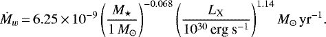
where t and r are the temporal and radial coordinates, Σgas is the gas surface density, and ν = αcsHgas the kinematic viscosity given by the dimensionless parameter α (Shakura & Sunyaev 1973), the local sound speed (cs), and the scale height of the disc (Hgas).  is the sink term due to the X-ray photoevaporation by the central star computed following Owen et al. (2012), who derived analytical prescriptions from radiation-hydrodynamic models (Owen et al. 2010, 2011). For full or primordial discs, the fit to the total mass-loss rate as a function of the stellar mass and X-ray luminosity is given by
 (2)
(2)
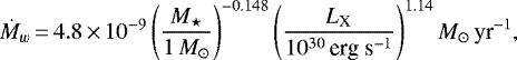
At some point, a gap is opened in the gas disc at a radial distance of a few astronomical units, and the gas inside this region is rapidly accreted by the central star. Once the gas inside the location in which the gap opened is completely drained, the disc becomes a transitional disc (i.e. has an inner hole). More precisely, we define this transition once the gas at each radial bin inside the gap is below Σgas = 10−5 g cm−2. The mass-loss rate is then computed as
 (3)
(3)
where, following Preibisch et al. (2005), LX is the X-Ray luminosity of the star, as
![Mathematical equation: \begin{equation*} \textrm{log}(L_{\textrm{X}}[\textrm{erg~}\textrm{s}^{-1}])\,{=}\,30.37 + 1.44\,\textrm{log}(M_{\star}/M_{\odot}). \end{equation*}](/articles/aa/full_html/2020/12/aa39140-20/aa39140-20-eq5.png) (4)
(4)
From normalised radial mass-loss profiles (see Eqs. (B2) and (B5) of Owen et al. 2012) and with Eqs. (2) and (3) we can compute  which verifies
 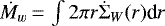 . The disc is resolved from 0.05 to 1000 au using 2000 radial bins logarithmically equally spaced.
Following observations (Andrews et al. 2010), the initial gas surface density is taken as:
 (5)
(5)
where rc is the characteristic or cut-off radius and  is a normalisation parameter that depends on the disc mass. We adopt rc = 39 au and γ = 0.9, which are the mean values of the distributions inferred from observations (Andrews et al. 2010). We vary the total disc mass from 0.01 to 0.1 M⊙ and the viscosity parameter adopts values of α = 10−5, 10−4, 10−3.
2.2 Dust evolution
As in Guilera et al. (2020), the evolution of dust along the disc is computed following the approach presented in Dra̧zkowska et al. (2016) and Drążkowska & Alibert (2017), which is based on the results of Birnstiel et al. (2011, 2012). In this model, the maximum size of the dust particles at each radial bin is limited by dust coagulation, radial drift, and fragmentation. The dust properties change at the water ice line, which is defined at the place where the midplane temperature equals 170 K. The ice line moves inwards as the disc cools.
The maximum particle size at a given time is given by:
 (6)
(6)
where  is the initial dust size. We note that at each radial bin and each time-step there is a dust or pebble size distribution between 1 micron and
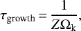
  given by Eq. (6). τgrowth is the collisional growth timescale
 (7)
(7)
with Z = Σd∕Σgas being the dust-to-gas ratio, and Ωk the Keplerian frequency. The maximum size of dust particles limited by radial drift is given by
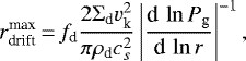 (8)
(8)
where fd = 0.55 (Birnstiel et al. 2012), vk is the Keplerian velocity, Pg the gas pressure, and ρd is the mean dust density, taking values of ρd = 3 g cm−3 and ρd = 1 g cm−3 inside and outside the ice line, respectively. These values assume a pure silicate composition for the grains within the ice line and of a mixtureof ices and silicates beyond it (Drążkowska & Alibert 2017). The maximum size of dust particles limited by fragmentation is:
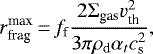 (9)
(9)
where ff = 0.37 (Birnstiel et al. 2011), and we use a fragmentation threshold velocity vth = 1 m s−1 for silicate dust and vth = 10 m s−1 for icy dust(Drążkowska & Alibert 2017). The turbulence strength parameter, αt, affects the impact velocity of dust particles and their settling. In principle, this quantity could differ from the α viscosity. However, as in our disc model the angular momentum transfer is driven by turbulent viscosity, we consider αt = α throughout this work (as assumed by previous studies, e.g. Ormel & Kobayashi 2012; Drążkowska & Alibert 2017; Guilera et al. 2020).
Equation (9) considers that fragmentation is driven by the turbulent velocities. However, if the viscosity in the disc midplane becomes very low, fragmentation could be driven by differential drift. The maximum particle size in this case is given by (Birnstiel et al. 2012)
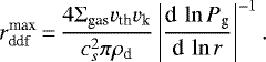 (10)
(10)
The dust is strongly coupled to the gas, and this is why the time evolution of the dust surface density, Σd, is calculated via an advection-diffusion equation,
![Mathematical equation: \begin{equation*} \frac{\partial}{\partial t} \left(\Sigma_{\textrm{d}}\right) + \frac{1}{r} \frac{\partial}{\partial r} \left(r \,\overline{v}_{\textrm{drift}} \,\Sigma_{\textrm{d}} \right) - \frac{1}{r} \frac{\partial}{\partial r} \left[ r \,D^{*} \,{\Sigma_{\textrm{gas}}} \frac{\partial}{\partial r} \left(\frac{\Sigma_{\textrm{d}}}{{\Sigma_{\textrm{gas}}}} \right) \right]\,{=}\, \dot{\Sigma}_{\textrm{d}},\end{equation*}](/articles/aa/full_html/2020/12/aa39140-20/aa39140-20-eq17.png) (11)
(11)
where  represents the sink term due to planet accretion and pebble sublimation. We consider that when inward-drifting pebbles from the outer part of the disc cross the ice line, they lose 50% of their mass. D* = ν∕(1 + St2) is the dust diffusivity (Youdin & Lithwick 2007), and St = πρdrd∕2Σgas the mass-weighted mean Stokes number of the dust size distribution. rd represents the mass-weighted mean radius of the dust-size distribution, given by
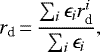 (12)
(12)
with  being the radius of the dust particle of the species i, and
  the ratio between the volumetric dust density of the species i and the volumetric gas density (see Guilera et al. 2020). We note that because the mean size is mass weighted, the maximum and mean sizes are very similar, as shown in Appendix A of Guilera et al. (2020). To compute the weighted mean-drift velocities of the pebble population (
 ), we follow the same approach as in Guilera et al. (2020), considering the reduction in the pebble drift velocities by the dust-to-gas back-reaction as being due to the increment in the dust-to-gas ratio (see Guilera et al. 2020, for details).
The initial dust surface density is given by
 (13)
(13)
where ηice takes into account the sublimation of water-ice and adopts values of ηice = 1/2 inside the ice line and ηice = 1 outside of it (Lodders et al. 2009). We adopt Z0 = 0.01 as the initial dust-to-gas ratio of the nominal runs (Table 1 summarizes the values adopted for the disc parameters in our simulations).
Figure 1 shows an example of gas and dust evolution. The upper and lower left panels correspond to the evolution of the gas surface density, midplane temperature, and aspect ratio. The bottom right panel shows the evolution of the surface density of dust. We note that photoevaporation carves a gap in the mid-disc, at ~2 Myr for thisparticular case. Once the gap opens, dust from the outer disc cannot reach the inner regions of the system any longer. This leads to a dust accumulation at the outer edge of the gap, which is visible as vertical lines. A similar dust behaviour in photoevaporating discs was reported in Ercolano et al. (2017).
Disc parameters that we vary and the values adopted.
2.3 Pebble accretion
The initial micrometre-sized dust grows to millimetre(mm)- to centimetre(cm)-sized pebbles during the disc evolution1. These pebbles can be effectively accreted by embryos present in the disc. We follow the growth of a Moon-mass embryo (MP = 0.01 M⊕) by pebble accretion.
To introduce the pebble accretion rate it is first useful to define the pebble scale height (Youdin & Lithwick 2007):
 (14)
(14)
We note that the pebbles will be more concentrated towards the disc midplane if the disc is rather laminar (low α) and/or if the Stokes number is large. In this case, the pebble accretion occurs in a 2D fashion and for St < 0.1 its rate is given by (Lambrechts & Johansen 2014):
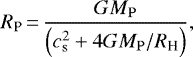
 (15)
(15)
where RH is the Hill radius of the planet, vH the Keplerian velocity at a distance of the Hill radius from the centre of the planet, ΣP the surface density of pebbles at the position of the planet, and St is the Stokes number of the particles at the position of the planet. For 0.1 < St < 1, Eq. (15) must be evaluated with St = 0.1.
Pebble accretion becomes 3D if:
 (16)
(16)
In this case, the accretion of pebbles is given by the slower 3D rate (e.g. Brasser et al. 2017):
 (17)
(17)
We note that the lower the Stokes number, the easier it is for f3D to be smaller than 1, and therefore the more likely it is that pebble accretion happens in 3D. For example, for St = 0.01, 2D pebble accretion occurs once the Hill radius exceeds approximately 3.4 pebble scale heights; for St = 10−4, RH is required to be 16 Hpeb. Indeed, because of the low Stokes number within the water ice line for α ≥ 10−4, pebble accretion occurs always in 3D for those cases. The same was reported in Lambrechts et al. (2019).
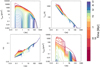 |
Fig. 1 Evolution of the gas surface density (top left), midplane temperature (top right), aspect ratio (bottom left), and dust surface density (bottom right) of the disc with α = 10−4 and Md,0 = 0.06 M⊙. The disc profiles are shown every 6 × 10⁴ yr. The dip on the dust surface density at 0.2 au is due to the presence of a growing planet at that location. |
2.4 The pebble isolation mass
A planetary embryo can grow by accreting pebbles until its mass is large enough to perturb the disc and create a pressure bump beyond the orbit of the protoplanet. Hydrodynamical simulations find that the pebble isolation mass can be approximated as follows (Lambrechts et al. 2014, hereafter L14):
 (18)
(18)
More sophisticated prescriptions were found by Bitsch et al. (2018, hereafter B18):
![Mathematical equation: \begin{align*} {M_{\rm{iso}}}\,{=}&\,25 \left(\frac{H_{\textrm{gas}}/r}{0.05} \right)^3 \left[ 0.34 \left(\frac{ \textrm{log}(0.001)}{ \textrm{log}(\alpha)} \right)^4 + 0.66 \right]\nonumber\\ &\times\left[ 1- \frac{ \frac{\partial {\textrm{ln}} P}{ \partial {\textrm{ln}} r }+ 2.5}{6} \right] \ {M}_{\oplus} ,\end{align*}](/articles/aa/full_html/2020/12/aa39140-20/aa39140-20-eq29.png) (19)
(19)
and Ataiee et al. (2018, hereafter A18):
 (20)
(20)
In Fig. 2, we show a comparison of the different definitions of pebble isolation mass for the different prescriptions for a disc of α = 10−4. We note that the expressions of L14 and B18 give remarkably similar values, while that of A18 gives lower values. The pebble isolation mass from A18 would only surpass that of L14 for α ≥ 7.4 × 10⁻³, and for such high viscosities the cores do not grow because of the extremely low Stokes number (see Sect. 3.1). The same reasoning can be applied for the prescription provided by B18 for α ≳ 10−4. As the cores grow only for α ≲ 10−4, and for those viscosities L14 gives the maximum possible Miso, we adopt Miso from Eq. (18) throughout this work.
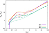 |
Fig. 2 Pebble isolation mass along the disc of Md,0 = 0.06 M⊙ and α = 10−4 at 20 kyr (solid), 1 Myr (dashed), and 2 Myr (dotted) of disc evolution. The purple curves correspond to the expression of Miso found by B18, green curves to that found by A18, and orange curves to that found by L14. The inner border of the disc is defined at a = 0.05 au. |
2.5 Gas accretion
In this section we describe the way we compute gas accretion before and after the pebble isolation mass is reached by the protoplanet.
2.5.1 Attached phase
We compute the gas accretion by solving the standard planetary internal structure equations, assuming a uniform luminosity that results from the accretion of solids and envelope contraction (see Alibert et al. 2013; Venturini et al. 2016; Venturini & Helled 2020, for details).
The internal structure equations are solved using as boundary conditions the pressure and temperature of the protoplanetary disc at the position of the planetary embryo and defining the planetary radius as a combination of the Hill and Bondi radii, as suggested by 3D hydrodynamical simulations (Lissauer et al. 2009):
 (21)
(21)
where cs is the sound speed in the protoplanetary disc at the location of the planet, a, and RH is the Hill radius. We assume that the solids reach the core, meaning that the envelope keeps a H-He composition, and we implement the EOS of Saumon et al. (1995). We define the envelope opacity as κ = fdust κgr + κgas (e.g. Ikoma et al. 2000), where the grain opacity is taken from Bell & Lin (1994), and the gas opacity from the tables of Freedman et al. (2014). The grain opacity from Bell & Lin (1994) corresponds to small grain sizes, typical of the ISM. fdust is a reduction factor to account for the decrease in grain opacity caused by grain growth and settling within the envelope. Studies show that this reduction factor can be typically ~0.01 (e.g. Movshovitz et al. 2010; Mordasini 2014). However, recent work suggest that after attaining Miso, the dust opacity might actually increase due to the trapping of the largest pebbles at the pressure bump (Chen et al. 2020). We are interested in finding the maximum mass of a rocky core to trigger substantial gas accretion, which is why we stick to conservatively high dust opacities and take fdust = 1 when solving the internal structure.
After the pebble isolation mass is reached, the resolution of the internal structure equations with uniform luminosity becomes unstable because of the proximity to critical mass. Therefore, at this stage we adopt the classical gas accretion rates of Ikoma et al. (2000), which are suited to the cases of no solid accretion, like ours. The prescription is given by the timescale of gas accretion, which depends on the core mass and dust opacity:
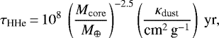 (22)
(22)
from which the gas accretion rate is computed as ṀHHe = MHHe∕τHHe. We note that in Eq. (22) the dust opacity is constant throughout the envelope, and it takes values of κdust = fdust cm2 g−1 for T ≤ 170 K, and of κdust = 0.22 fdust cm2 g−1 for 170 < T < 1600 K (Ikoma, priv. comm.). Therefore, as our simulations assume ISM opacities and take place within the water ice line, κdust = 0.22.
We emphasise the importance of computing the internal structure equations immediately after reaching the pebble isolation mass, because an increase of approximately one order of magnitude in the envelope mass occurs once the solid accretion is shut down. This happens because of the loss of thermal support originated by the pebble luminosity. More precisely, the critical mass is achieved when the luminosity due to the envelope contraction reaches a minimum (Ikoma et al. 2000). In practice however, to guarantee continuity in the gas accretion rate, we switch to Ikoma’s prescription when this rate and the one obtained from solving the internal structure are equal.
2.5.2 Detached phase
At a certain point the gas accretion required by the protoplanet’s thermal structure exceeds the amount that can be supplied by the disc. At this stage the protoplanet “detaches” from the disc and continues accreting gas at the rate of the disc viscous accretion:
 (23)
(23)
Mathematically, gas accretion is therefore given by
 (24)
(24)
Once in the detached phase, gas accretion can be damped even further if a gap opens in the gas disc. This occurs when (Crida et al. 2006)
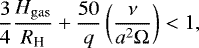 (25)
(25)
where q = MP∕Mstar. When the gap opens, gas accretion reduces even further and is computed following Eqs. (36)–(39) of Tanigawa & Ikoma (2007).
2.6 Embryo location and migration
Despite the fact that planet–disc interactions are expected to cause migration, some mechanisms, such as for example the presence of pressure bumps, can trap protoplanets at a fixed location (e.g. Guilera & Sándor 2017). In particular, Flock et al. (2019) showed that the silicate ice line can create such a maximum, halting planetary migration at orbital periods of ~10–22 days. For our nominal setup, we assume in-situ formation at a = 0.2 au. This position corresponds to an orbital period of 33 days for a solar-mass star, and is representative of the location where many super-Earths/mini-Neptunes are observed. We also study in situ formation at a = 0.1 and a = 1 au in Sect. 3.3.1.
In addition, we study the possibility of migration from just inside the ice line in Sect. 3.3.2. The Type-I migration prescription adopted corresponds to the one derived by Jiménez & Masset (2017) and Masset (2017), which includes the possibility of outward migration due to corotation and thermal torques, although outward migration does not take place in the cases studied in this work. Planets switch to type-II migration once a partial gap opens in the gaseous disc (Eq. (25)) and migrate according to Ida & Lin (2004) or Mordasini et al. (2009) depending on whether they are in the “disc-dominated” or “planet-dominated” type-II migration regime (Armitage 2007).
2.7 Post-formation atmospheric mass loss
After the end of the formation phase, we follow the thermodynamic evolution (cooling and contraction) of the individual planets over gigayear timescales, including the effect of XUV-driven atmospheric photoevaporation. This in particular yields the radii of the planets at 5 Gyr as an important observable quantity. The planet evolution model described in detail in Mordasini et al. (2012); Jin et al. (2014), and Mordasini (2020) solves the classical spherically symmetric planetary internal structure equations. The equation of state (EOS) for the iron-silicate core is the modified polytropic EOS of Seager et al. (2007). The EOS of the gaseous envelope is the new H/He EOS of Chabrier et al. (2019). The outer (atmospheric) boundary condition is given by the semi-grey model described in Jin et al. (2014). The opacities are given by the condensate-free opacity tables of Freedman et al. (2014). In contrast to the formation phase, grain opacities are now neglected, as grains quickly settle into the interior once gas accretion stops (Mordasini 2014). When calculating the luminosity evolution, the gravitational and internalenergy of the core and envelope as well as radiogenic heating are included (see Linder et al. 2019). Atmospheric escape rates are found by interpolating in the grid of evaporation rates provided by Kubyshkina et al. (2018). These evaporation rates were obtained with the upper atmosphere hydrodynamic code of Erkaev et al. (2016). The code solves the 1D equations for mass, momentum, and energy conservation and accounts for Lyα cooling, XUV heating, andH cooling. Thestellar XUV luminosity as a function of time is taken from MacDonald et al. (2019).
3 Results
Here we present results considering different disc mass, viscosity, metallicity, and formation locations.
3.1 The key role of viscosity
We start by showing the results of our nominal case, defined as in-situ growth for an embryo located at a = 0.2 au from the Sun (or orbital period of 33 days). The dust-to-gas ratio of the initial disc is taken as Z0 = 0.01. The results for this setup are summarised in Fig. 3. We highlighted the cases with different colours: grey shows simulations where the planet practically does not grow and ends up with a mass on the order of magnitude of that of the Moon. Green marks rock-dominated planets, which are defined as having a final planet mass larger than that of Mars and a H-He mass fraction of fHHe < 50%. Finally, we show gas-dominated planets in yellow, which are defined as having fHHe ≥ 50%. We note that the output of the simulations is extremely sensitive to the assumed α. In discs with α = 10−3, the initial moon-mass embryo barely grows at all, for any disc mass.
In general, the trend of Fig. 3 is that the final planet mass increases the lower the viscosity and the larger the initial disc mass. Why does this happen? When we analyse the evolution of the pebble sizes along the disc (Fig. 4, upper panel), we see that inside the water ice line, the larger the viscosity, the lower the particle size. Inside the water ice line the fragmentation threshold velocity is low (vth = 1 m s−1), implying a maximum particle size limited by fragmentation. Turbulence promotes fragmentation (Eq. (9)), and therefore, the larger the α, the smaller the pebble size. From the definition of the Stokes number, it is clear that the lower the particle size, the lower its Stokes number. We observe this in the lower panel of Fig. 4. Because of fragmentation, the Stokes number decreases by one order of magnitude when α increases by the same amount. The Stokes number affects the pebble accretion rate in two ways. First, it enters directly into Eqs. (15)–(17). The lower the Stokes number, the lower the pebble accretion rate. Second, it affects the surface density of pebbles, which also enters in Eq. (15).
The top panel of Fig. 5 displays the surface density of pebbles as a function of time, which results from solving the advection–diffusion equation (Eq. (11)). We note that both the behaviour of Σpeb and stokes number promote core growth for low viscosities. As long as the Stokes number is lower than 1, the lower its value, the lower the drift velocity (see Eqs. (11–16) in Guilera et al. 2020). This means that the pebble flux will decrease with increasing α. This is shown on the central panel of Fig. 5, where we compare pebble fluxes for the different α of the disc with Md,0 = 0.06 M⊙. From this figure it is clear that the pebble flux is not constant, varying by up to two to three orders of magnitude as the disc evolves. Importantly, for all cases the pebble flux and the surface density of pebbles decays abruptly at ~2–2.5 Myr of disc evolution. This occurs because a gap in the mid disc is carved by photoevaporation shortly before this point in time (see Table 2 and e.g. top-left and bottom-right panels of Fig. 1), and so the pebble supply from the outer disc is shut down. The bottom panel of Fig. 5shows the integrated pebble flux for the same cases, in other words, the total amount of pebbles that passed through the position of the planet until a given time. We note that an integrated pebble flux greater than 190 M⊕, which is needed to form “true” Super-Earths (MP > 5 M⊕) in the work of Lambrechts et al. (2019), is never achieved. This explains why our results favour the formation of terrestrial planets by dry pebble accretion, and not of super-Earths. In addition, we note that after only 1 Myr of disc evolution, the amount of pebbles at 0.2 au has already receded so strongly that any substantial core growth beyond that time is unfeasible, as shows Fig. 6. The top panel of Fig. 6 shows the pebble accretion rate onto the protoplanet for the same cases as those shown in Fig. 5. These accretion rates always occur in 3D. We note that the pebble accretion rate varies by up to four orders of magnitude between α = 10−5 and α = 10−3. This explains the differentoutputs of the nominal setup displayed in Fig. 3. We note that in Fig. 6 the pebble accretion rate for α = 10−5 drops abruptly at t = 5 × 10⁴ yr despite a large pebble flux still existing at that time. This happens because the planet reaches the pebble isolation mass at that early time, as can be seen more easily in the bottom panel of the same figure. For α = 10−4 the pebble isolation mass is reached late, at t = 3.7 Myr, when the core no longer grows by any appreciable amount because of the natural decline in the pebble flux. On the contrary, for α = 10−5 the pebble accretion rate is extremely high, and Miso is reached within the first 46 000 yr of disc evolution. This means that most of the pebbles that continue drifting through the orbit of the planet cannot contribute to its growth.
Let us analyse now the results of the nominal setup (Fig. 3) for each choice of α viscosity. As explained above, for the cases where α = 10−3, the turbulence fragments the pebbles into small dust particles (~10−100 μm), which translates into almost negligible pebble accretion rates. This is why these cores remain as approximately lunar-mass embryos. However, it is interesting to note that contrary to the other viscosities, the core mass increases slightly more for lower disc masses. More precisely, the small amount of growth reported in the table happens just after photoevaporation opens a gap in the mid-disc and the gas of the inner disc starts to disappear. At that point the decrease in the gas surface density allows the small particles that are within the Hill sphere of the embryo (there are still particles around because they drift very little due to their small size) to increase their stokes number, fostering pebble accretion for a very short time. For lower disc masses, this happens earlier, when there are typically more pebbles around. This explains thetrend in the final embryo masses. This effect almost does not occur for other viscosities because by the time the Stokes number starts to increase because of gas depletion, the pebble isolation mass is already attained.
Interestingly, the stall of growth for α = 10−3 occurs despite the initial dust-to-gas ratio, and also for migrating planets, as we show in the following sections. We can therefore conclude that discs with intermediate and high turbulence (α ≥ 10−3) cannot formplanets by pebble accretion inside the water ice line.
For discs where α = 10−4, the planet mass varies from 0.25 M⊕ for the lowest initial disc mass (Md,0 = 0.01 M⊙) to 1.95 M⊕ for the initial highest one (Md,0 = 0.1 M⊙). For the two lowest disc masses, the pebble flux stops before the pebble isolation mass is reached because the disc runs out of pebbles. Forthe two highest disc masses, the pebble isolation mass is reached close to the disc dispersal, when Miso is low. This shows the importance of considering the physical dimensions of discs, because the final core mass of planets formed by pebbles can be determined by the halt in the pebble supply and not solely by the attainment of the pebble isolation mass.
For discs where α = 10−5, the flux of pebbles and the pebble-accretion rates are very high, and so the pebble isolation mass is rapidly achieved. This sets the final core mass shown in Fig. 3 for this α. These cases of extremely low viscosity show the formation of two types of planets: either rocky super-Earths of masses below 5 M⊕, or “gas-dwarfs” for the two largest initial disc masses. We use the term gas-dwarf to refer to planets whose envelopes contribute greatly to the total mass, that is, fHHe ~ 50%. These gas-dwarfs are very interesting objects, as they have a gas-to-core ratio of almost unity. These planets do not explode into gas giants because of the opening of a gap at low masses caused by the low disc viscosity (see Eq. (25)) and the low disc aspect ratio at short orbital distances. This halts gas accretion at MP≳ 8 M⊕ (see dashed-purple line in the bottom panel of Fig. 6). Since these planets occur only at high disc masses and extremely low (probably unrealistically low) disc viscosities, they should rarely occur in nature.
We close this section by analysing the efficiency of pebble accretion for the nominal setup. Such efficiency can be defined as the ratio between the final core mass and the integrated pebble flux at the end of the simulation (Guillot et al. 2014; Lambrechts & Johansen 2014). This is shown in the last column of Table 3 and is represented by ɛ. We note that the integrated pebble flux is always smaller than the initial amount of dust in the disc. Indeed, many of the outer pebbles do not reach the orbit of the planet; once photoevaporation opens a gap in the mid-disc, the inner disc becomes detached from the outer one and the pebbles coming from far away can no longer reach a planet growing in the inner disc. In addition, the different α set different mean sizes for the dust and pebbles, which translates into very different drift speeds. The larger the α, the smaller the grains and the less they drift. This explains the trend of the reduction of the integrated pebble flux with increasing α. The low pebble accretion efficiencies that we find are in general agreement with the results of Ormel & Liu (2018). For the lowest disc masses of the cases with α = 10−3 our efficiencies are larger, but, as explained above, this is caused by photoevaporation, which is not taken into account in Ormel & Liu (2018).
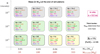 |
Fig. 3 Summary of results for the nominal setup at the end of the simulations as a function of the initial disc mass and α-viscosity. The horizontal axis also shows the initial mass of dust in the disc. MP denotes the total planet mass, Mcore the core mass, Menv the mass of H-He envelope, and Mpeb the total mass of pebbles that drifted through the position of the embryo. All masses in the squares are in M⊕. fHHe is the mass fraction of H-He of the planet as a percentage. Cases where planets remain as lunar-mass embryos are colored in grey. Planets that are rocky-dominated (fHHe < 30%) and gas-dominated (fHHe > 30%) with masses larger than that of Mars are highlighted in green and yellow, respectively. Boxes with thick borders indicate that the core growth was truncated by reaching the pebble isolation mass (see also Table 3). |
Discs characteristics: gas and dust evolution for the nominal setup (Z0 = 0.01).
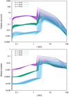 |
Fig. 4 Evolution of maximum pebble (or dust) size (top) and Stokes number (bottom) along the disc of Md,0 = 0.06 M⊙. The profiles are shown every 80 Kyr and until photoevaporation carves a gap in the middle of the discs, halting pebble drift. The change of behaviour at ~1–3 au is due to the change in pebble properties at the water ice line. |
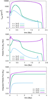 |
Fig. 5 Evolution of the pebble surface density (top), the pebble flux (middle), and the integrated pebble flux (bottom) of the disc with Md,0 = 0.06 M⊙ of the nominal setup (Fig. 3). The pebble flux ceases once the gap due to photoevaporation is carved at a ≈ 3− 4 au (see Fig. 1). |
Pebble flux and isolation mass for the nominal setup (Z0 = 0.01, a = 0.2 au).
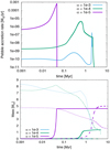 |
Fig. 6 Evolution of the pebble accretion rate (top) and planet growth (bottom) for the same cases as in Fig. 5 (disc of Md,0 = 0.06 M⊙ of the nominal setup). Bottom panel: the solid lines show the growth of the core, the dashed lines the growth of the envelope, and the dotted thin lines the evolution of the pebble isolation mass foreach case. The accretion rate of pebbles is shut down very early for the case of α = 10−5 because Miso is attained. |
3.2 Dependence on the initial dust-to-gas ratio or stellar metallicity
Exoplanets with periods shorter than 100 days exist around stars with a wide range of stellar metallicities, spanning in [Fe/H] from −0.5 to +0.5 dex (e.g. Buchhave & Latham 2015). This motivates us to study rocky planet formation for different disc metallicities, which presumably are representative of the star metallicity at the time of formation of the system.
We repeated our runs for an initial dust-to-gas ratio of Z0 = 0.005, which, taking the protosolar abundances of Z⊙ = 0.0153 (Lodders et al. 2009), corresponds to a metallicity of [Fe/H] ≈−0.486. This is an extremely low stellar metallicity, representative of the lowest values of stars-hosting planets (Ghezzi et al. 2010). The output of this setup is summarised in Fig. 7. We see that in this case, α = 10−3 continues leading to almost no growth. For α = 10−4, three out of four cases lead to the Mars-mass embryos. The case of extreme low viscosity of α = 10−5 is very similar to the nominal one. This is a trend for any disc metallicity, and is caused by the rapid attainment of the pebble isolation mass, which does not vary by changing Z0 because it only depends on the aspect ratio of the disc.
We also repeated the simulations for a high initial dust-to-gas ratio of Z0 = 0.03, corresponding to [Fe/H] ≈ 0.292. Furthermore, our results do not change for metallicities higher than this. The results are summarised in the lower panel of Fig. 7. Again, when α = 10−3, planetary seeds do not grow beyond Moon-mass. For α = 10−4, the two lowest disc masses form terrestrial planets. For the two highest disc masses, the cores grow larger than 5 M⊕ and accrete substantial envelopes.
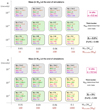 |
Fig. 7 Same as in Fig. 3 but for a low (Z0 = 0.005) and a high (Z0 = 0.03) initial dust-to-gas ratio. |
3.3 Terrestrial planet formation for different embryo locations
We performed the same simulations assuming different initial locations for the embryo. We first analyse two other cases of in-situ growth, and then one case where the embryo is allowed to migrate from just inside the water ice line.
3.3.1 In-situ growth
When repeating the calculations shown in Fig. 3 for a = 0.1 au and a = 1 au, we find that the typical outcome of terrestrial planets for α = 10−4 also holds for different semi-major axis as shown in Fig. 8. The results are not particularly sensitive to embryo location (as long as it lays within the ice line) because the pebble surface density tends to increase for shorter orbital periods (e.g. bottom-left panel of Fig. 1), while the opposite is true for the Stokes number (Fig. 4).
For α = 10−5, we note that the mass fraction of H-He increases for larger semi-major axis. This is related to the increase in the aspect ratio for longer orbital periods, as shown in the bottom-left panel of Fig. 1. The larger the H∕r, the more massive a planet can grow without opening a gap. We illustrate the link between the evolution of the aspect ratio and planet mass for a planet growing at a = 1 au, a = 0.2 au, and a migrating case in Fig. 9. All these cases reach Mcore ~ 7 M⊕, but despite having the same viscosity of α = 10−5, the final masses reach different values due to the difference in aspect ratio.
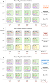 |
Fig. 8 Same as Fig. 3 but for the planet growing at different locations. Top and middle panels: assume in-situ growth at 0.1 and 1 au, respectively. Bottom panel: planets start at 0.2 au from the ice line (inside it) and are allowed to migrate. The range of semi-major axis of each box (in purple) indicates the initial and final planet location. |
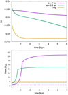 |
Fig. 9 Evolution of aspect ratio at the planet’s location (top), and planet mass (bottom) for three cases where Md,0 = 0.1 M⊙ and α = 10−5. The dashed lines indicate the evolution of Mcore and the solidlines the evolution of MP. The planet’s location is specified in the legend. For the migrating case, the evolution of a is shown in the next figure. |
3.3.2 Migration from the ice line
Finally, we also tested the possibility of planetary migration. For these runs the embryos start at 0.2 au from the ice line (inside the ice line to keep them dry by construction). The initial ice line location depends on the mass of the disc and on the value of the α parameter, and so it is different for each disc. All the planets that migrate and reach a planet mass larger than 1 M⊕ migrate fast and park close to the inner edge of the disc, where a pressure bump exists due to the zero-torque boundary condition at the inner edge of the gas disc. We find the same trends as before, apart from the fact that more rocky-dominated planets are produced for α = 10−5. Indeed, for the highest disc mass, a rocky planet with Mcore = 7 M⊕ is formed. The halt of gas accretion for this massive core is related to the low scale height of the disc at shorter orbital periods, as explained above. Figure 10 shows that soon after attaining isolation mass, this planet opens a gap at Menv ≈ 0.1 M⊕. At this time the planet switches from type I to type II migration, moving slower until parking at the inner edge of the disc. We note that gas accretion stops earlier than this because of the low accretion rates with gap opening given by Tanigawa & Ikoma (2007) (dashed-green lines). We study the migration scenario in more depth in an accompanying letter (Venturini et al. 2020a, hereafter, Paper II).
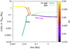 |
Fig. 10 Evolution of semi-major axis (yellow-purple) and envelope mass (green curve) for the migrating case of Fig. 9. The point in time when the isolation mass is reached is marked with a black dot. The planet transitions from type I to type II migration when the gap opens (light green curve). The dashed curves indicate that gas accretion follows Tanigawa & Ikoma (2007). |
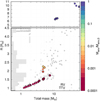 |
Fig. 11 Final mass vs. radius for all the planets with P < 100 days and Mcore ≥ 1 M⊕, represented by coloured circles outlined in black. The coloured circles outlined in grey represent the planets computed with low dust opacity (Sect. 4.2). The colours show the final envelope mass relative to the initial one. The final masses of the envelopes and radii are computed as in Sect. 2.7. The grey small dots/triangles represent the RV/TTV planets used by Zeng et al. (2019; from their Fig. 2 and Table S1) and were used to construct the grey histogram on the left, which depicts the percentage of planets as a function of their radius. |
3.4 Planetary radii
We are interested in understanding how silicate-pebble accretion contributes to the formation of super-Earths/mini-Neptunes. Out of the 60 planets we form with orbital periods below 100 days (i.e. considering all results except in-situ formation at a = 1 au), 30 accrete a core more massive than 1 M⊕ and, for those, we show the final mass–radius plot, constructed as in Sect. 2.7, in Fig. 11. Of those 30 planets, 23 finish with radii below 1.8 R⊕, that is, most of the super-Earths we form contribute to the first peak of the Kepler size distribution. One planet of those 30 falls exactly in the valley, with a radius of 1.96 R⊕, and two fall on the second peak with RP ≈ 2.2−2.3 R⊕. These last three cases correspond to planets with Mcore ≈ 4.6−5.1 M⊕ which had originally an envelope of equal mass and lost most of it, ending up with a final envelope mass of 5.5 × 10⁻³ M⊕ for the planet inthe valley and 2–3 × 10⁻² M⊕ for the two planets on the second peak.
Interestingly, 3 of these 30 planets have a radius between 6.5 and 6.7 R⊕. These objects have cores of approximately 7 M⊕, and started with envelopes of equal mass and finished with envelopes in the range of 3–5 M⊕. These three cases are planets originating in extremely low-viscosity discs (α = 10−5) and are therefore expected to be rare. Finally, the only true gas giant we formed (Mcore = 7.4 M⊕, Menv = 51 M⊕, α = 10−4) loses barely ~1% of its original envelope and finishes with a radius of 9.7 R⊕.
Allplanets with Mcore ≥ 1 M⊕ which retain some H-He after 5 Gyr of evaporation-driven mass loss.
4 Discussion
4.1 Implications for the Kepler size distribution
By studying planet formation by dry pebble accretion with pebbles growing self-consistently from initial micrometre dust, we find that out of 72 simulations, 35 cases lead to the formation of rocky-dominated planets (green squares in Figs. 3, 7 and 8), of which 34 remain as naked cores after 5 Gyr of evolution. The masses of these bare cores range typically from that of Mars to 4 M⊕. These planets contribute to the first peak of the Kepler size distribution. The only case of these rock-dominated planets that retains some atmosphere after evolution is a core that reaches 4.98 M⊕ at a = 1 au (see Table 4), which, because of the low irradiance, retains 93% of the original 0.51 M⊕ envelope, leading to a planet radius of 3.17 M⊕. Special cases with Mcore > 4 M⊕ are migrating planets in extremely low-viscosity discs, which can remain as bare cores even for Mcore = 7.5 M⊕, as long as the planet ends with an orbital period as short as 4 days.
Out of the total of 72 cases, only 3 planets within a 100-day orbital period fall in the gap or on the second peak of the size distribution (see Table 4). Interestingly, these planets started as gas-dominated objects (or gas-dwarfs, i.e. being more than 50% H-He), but lost more than 99% of their envelope due to evaporation. Equally interesting, cores with ~7 M⊕ instead of 5 M⊕ lose considerably less H-He (~50%), yielding a planet radius of 6–7 R⊕ (see Fig. 11 Table 4). Several of these so-called sub-Saturns have been found (Petigura et al. 2018), and their origin poses challenges (Millholland et al. 2020).
Finally, we note that our silicate-pebble accretion model does not produce any planet with a size between 2.5 and 6 R⊕. Planets with sizes between 2.5 and 4 R⊕ are known to be very common (e.g Petigura et al. 2018, also clear from the observed exoplanets in Fig. 11). Our results suggest that those planets might not be dry. We address the origin of those objects in Paper II.
4.2 Dependence on the dust opacity
The fact that we cannot form planets ending up with radii between 2.5 and 6 R⊕ with our pure silicate-pebble accretion model could depend on our choice of opacities. In Sect. 2.5 we justify our choice of ISM opacities on the grounds of maximising the possibility of forming bare rocky cores.However, grain growth within the envelope could reduce the dust opacity by a factor of ~100 compared to ISM values (Mordasini 2014; Movshovitz & Podolak 2008). Thus, reduced opacities can lead to larger envelopes for equal core masses and hence could contribute to populating this range of RP ~ 2.5−6 R⊕.
To evaluate this possibility, we repeated 15 of our original simulations for those cases that would certainly lead to RP < 6.5 R⊕. The outcome of this test is presented in Table 5 and is shown with the coloured circles outlined in grey in Fig. 11.
Let us first note that a planet that ended up with Mcore ≈ 3 M⊕ has now an envelope mass after formation of Menv ≈ 20 M⊕ (sixth line of Table 5), contrary to the nominal case where Menv ≈ 0.03 M⊕ (Fig. 7). This is due to the rise of the gas accretion rate promoted by the lower opacities (Ikoma et al. 2000). Nevertheless, despite the thick envelope that the planet acquires with the low dust opacity, the envelope is completely removed by photoevaporation due to the low core gravity and relatively low overall planet gravity. The fact that similar cores that accreted very different envelopes can yield the same planetary radius after evaporation was pointed out by Mordasini (2020) as an obstacle to constrain the dust opacities from radii measurements. For larger core and envelope masses, the massive envelope accreted as a consequence of the low opacity can be retained after photoevaporation, now leading to a planet with Mcore ≈ 5 M⊕ and RP ≈ 10 R⊕ (fifth row of Table 5), compared with RP = 2.2 R⊕ of the nominal case (fifth row of Table 4). A similar result was found by Ogihara & Hori (2020), who assumed the envelopes to be dust-free. The planets that they form retain overly massive envelopes, which is why they find overly inflated planetary radii compared to the Kepler size distribution.
Overall, we note that the lower dust opacities also do not produce any planet in the size range of 2.5–6 R⊕ (Fig. 11 and Table 5). Either the thick envelopes are blown away by photoevaporation, leaving in the best case one planet in the second peak, or they are retained for sufficiently massive planets (MP ≳ 30 M⊕), yielding planetary radii above 6 R⊕. In Paper II, where we perform a larger number of simulations, we find some planets with RP ~ 2.5−6 R⊕, but these are typically migrated planets from beyond the ice line and are therefore ice-rich.
Low-dust-opacity cases (fdust = 0.01).
4.3 Dependence on the disc aspect ratio
One of our main findings is that pure rocky planets form with low masses, typically below 5 M⊕. The main property that sets this maximum mass is the pebble isolation mass (Lambrechts et al. 2014; Ormel 2017; Liu et al. 2019), which depends strongly on the aspect ratio of the disc (Eq. (18)), and therefore on the disc model. The low values of the pebble isolation mass that we find in the inner part of the disc correspond to aspect ratios of ~0.02–0.03 within 1 au (Fig. 1). The scale height of the disc depends on the thermodynamical state of the disc, which is determined by the heating and cooling processes at operation. We consider that the disc is heated by irradiation from the central star in addition to the heat produced by viscous accretion. The grain opacity is responsible for cooling the disc, and we used the opacity of Bell & Lin (1994), which corresponds to micrometre-sized grains. This is an upper bound for the grain opacity (Savvidou et al. 2020)2 and therefore maximises the disc scale height and the pebble isolation mass.
Despite the dependence of Miso on the disc model, other studies find similar values of pebble isolation mass to those found here. For instance, Liu et al. (2019) use a simple steady-state disc solution, and claim that planets grow up to a few Earth masses for an initial embryo location within 1 au. Bitsch et al. (2019), also via a steady-state disc solution, find that the disc structure normally leads to very small aspect ratios (around 2–2.5%) in the inner disc (within 1 au) at late times, leading to very small core masses of 1.6–3.0 Earth masses. Passive discs (Bitsch 2019) or discs with lower grain opacity (Savvidou et al. 2020) would yield even lower values of disc scale height, which reinforces our conclusion of pure rocky planets not being more massive than ≈ 5 M⊕ when formed by pebble accretion (neglecting post-disc N-body interactions).
4.4 Formation of rocky planets by planetesimal accretion
In this work we consider rocky planet formation driven solely by pebbles. Planetesimals might also form and contribute to the planetary growth (see Venturini et al. 2020b, and references there in), although in most of the cases we studied (α ≥ 10−4), the condition of streaming instability to form planetesimals (e.g Dra̧zkowska et al. 2016) is not fulfilled inside the water ice line. Nevertheless, other mechanisms that produce planetesimals could operate. For instance, Lenz et al. (2019) propose that hydrodynamical or magnetic instabilities could create turbulent structures along the entire disc that could clump solids triggering planetesimal formation. These latter authors propose a parameterised model in which planetesimals form by a local mechanism that converts a certain fraction of the pebble flux into planetesimals. Briefly, when the pebble flux becomes greater than a critical mass value over the lifetime of the turbulent structure, some fraction of the pebbles are transformed into planetesimals along the length scale of the turbulent structure. Thus, this mechanism is directly related to the local pebble flux instead of to the local dust-to-gas ratio as in the streaming instability mechanism. Lenz et al. (2019) showed that a high α-viscosity parameter (α = 10−2) does not allow the formation of planetesimal in the inner part of the disc, and that a moderate value (α = 10−3) generates steep planetesimal surface density profiles. Recently, Voelkel et al. (2020) introduced a model of dust growth and evolution, and the planetesimal formation model of Lenz et al. (2019) in a planet population synthesis model (Mordasini 2018). Voelkel et al. (2020) found that the steep planetesimal surface density profile generated by the pebble flux mechanism of Lenz et al. (2019) increases the rate of formation of terrestrial planets, super-Earths, and gas giants by the accretion of 100 km planetesimals in the inner region of the disc.
4.5 Growth by collisions after dispersal of the disc
Ogihara & Hori (2020) and Lambrechts et al. (2019) simulated the formation of super-Earths by both pebble accretion and N-body interactions. These studies show that the main driver of growth during the disc phase is the accretion of pebbles. Indeed, as pebble accretion is inefficient, meaning that most of the pebbles are not used to grow a planetary core (as we show in Table 3), when many embryos grow together there are enough pebbles for all and they all grow at similar rates (Ogihara & Hori 2020; Lambrechts et al. 2019). After disc dispersal, a super-Earth typically undergoes one or two giant collisions (Ogihara & Hori 2020). Therefore, if producing pure rocky planets of MP ≳ 5 M⊕ is atypical, pure rocky planets exceeding 10 M⊕ should also be unusual. This seems to be the case for the exoplanets discovered and analysed so far, specifically those that follow a pure rocky compositional mass–radius relation, as we discuss in Appendix D of Paper II.
4.6 Envelope enrichment
When the sublimation of the incoming solids is considered in core accretion, the amount of H-He that a core can bind changes (Hori & Ikoma 2011; Venturini et al. 2015, 2016; Brouwers & Ormel 2020). In principle, for uniform envelope metallicity, the increase of mean molecular weight makes the envelope more prone to contract, and therefore gas accretion is favoured (Venturini et al. 2016; Venturini & Helled 2017). However, when Z is not assumed to be uniform, and the resulting compositional gradient is calculated self-consistently, the heat transport is modified; the interior becomes hotter, which slightly abates gas accretion (Bodenheimer et al. 2018). Unlike water, silicates sublimate deeper in the envelope, and so a non-uniform Z is expected. According to the results of Bodenheimer et al. (2018), who are the only ones who have succeeded in including compositional gradients in formation models so far, when silicate enrichment is considered, a core of Mcore3 ≈ 7 M⊕ should bind an envelope containing MHHe = 0.37 M⊕, compared to MHHe = 0.68 M⊕ when silicate enrichment is neglected and all the solids are deposited in the core. In other words, the effect of silicate enrichment seems to give H-He masses of only a factor of two smaller. In light of these results, silicate pebble enrichment is not expected to substantially modify the H-He masses that we find in this work. Nevertheless, we consider that the inclusion of compositional gradients should be studied under much broader conditions to asses its true impact.
5 Conclusions
We studied pebble-driven planet formation inside the water ice line. For the first time, the pebble size and pebble surface density are computed self-consistently from dust growth and evolution calculations, instead of being prescribed as a free parameter as done by recent works (Lambrechts et al. 2019; Ogihara & Hori 2020). An important finding from this study is that pebble accretion is extremely sensitive to disc turbulence within the water ice line. This is a direct consequence of dust growth being limited by fragmentation in this region of the disc. Turbulence promotes fragmentation, which makes the silicate pebbles attain very different sizes for different viscosities. This has dramatic consequences for the planet growth. For intermediate viscosities of α = 10−3, the initial Moon-mass embryos show negligible growth. We find that the typical output of silicate pebble accretion for low viscosities (α ≲ 10−4) is terrestrial planets, that is, planets with a mass at the time of disc dispersal of between that of Mars and approximately three Earth masses. The formation of terrestrial planets by dry pebble accretion is very robust concerning disc metallicity and embryo location. Embryos growing in situ from 0.1 to 1 au or migrating from just inside the water ice line typically lead to terrestrial planets. In addition, discs with a very low initial dust-to-gas ratio of Z = 0.005 (which would correspond to the lowest-metallicity stars in the solar neighbourhood) can also produce terrestrial planets, but less massive, namely of ~0.1–0.5 M⊕.
Three factors limit the formation of purely rocky planets with masses exceeding ~5 M⊕. Firstly, the pebble isolation mass within the ice line decays typically fast to Miso ≲ 5 M⊕ within the first million years of disc evolution. Secondly, after approximately 1 to 3 Myr of disc evolution, photoevaporation carves a gap in the mid-disc. This truncates the supply of pebbles from the outer disc, halting the core growth. Finally, even if the core manages to grow quickly, for example in a very metallic disc and/or with extremely low viscosity, when Mcore ≈ 5 M⊕, the protoplanet is able to bind a substantial H-He envelope, in some cases so massive that the planets are no longer core-dominated, but resemble more a sub-Saturn or gas-dwarf.
Regarding the bi-modality of the Kepler size distribution, we find that all the rock-dominated planets that we form with mass below ~ 4 M⊕ lose their atmospheres completely and contribute to the first peak of the size distribution. A second small group of planets, with cores between 4 and 5 M⊕, end up with radius between 2 and 2.3 R⊕. These planets lost typically ~99% in mass of their original envelopes. Remarkably, for planets with orbital periods below 100 days, we do not obtain any object with size between ~2.5 and 6 R⊕. Our results show that rocky planets can sometimes contribute to the valley and the lower part of the second peak, but do not seem to be able to account entirely for the second peak. We study the origin of the second peak in an accompanying letter (Paper II).
Acknowledgements
We thank the anonymous referee for the criticism and enthusiasm about our work. We also thank B. Bitsch for his feedback and interest. J.V and O.M.G thank the ISSI Team “Ice giants: formation, evolution and link to exoplanets” for fruitful discussions. O.M.G acknowledges financial support from ISSI Bern in the framework of the Visiting Scientist Program. O.M.G. is partially support by the PICT 2018-0934 and PICT 2016-0053 from ANPCyT, Argentina. O.M.G. and M.P.R. acknowledge financial support from the Iniciativa Científica Milenio (ICM) via the Núcleo Milenio de Formación Planetaria Grant. M.P.R. also acknowledges financial support provided by FONDECYT grant 3190336. We thank J. Haldemann for technical help. This work has in part been carried out within the framework of the NCCR PlanetS supported by the Swiss National Science Foundation.
References
- Alibert, Y., Mordasini, C., Benz, W., & Winisdoerffer, C. 2005, A&A, 434, 343 [NASA ADS] [CrossRef] [EDP Sciences] [Google Scholar]
- Alibert, Y., Carron, F., Fortier, A., et al. 2013, A&A, 558, A109 [NASA ADS] [CrossRef] [EDP Sciences] [Google Scholar]
- Andrews, S. M., Wilner, D. J., Hughes, A. M., Qi, C., & Dullemond, C. P. 2010, ApJ, 723, 1241 [NASA ADS] [CrossRef] [Google Scholar]
- Armitage, P. J. 2007, ApJ, 665, 1381 [NASA ADS] [CrossRef] [Google Scholar]
- Ataiee, S., Baruteau, C., Alibert, Y., & Benz, W. 2018, A&A, 615, A110 [NASA ADS] [CrossRef] [EDP Sciences] [Google Scholar]
- Batalha, N. M., Rowe, J. F., Bryson, S. T., et al. 2013, ApJS, 204, 24 [NASA ADS] [CrossRef] [Google Scholar]
- Bell, K. R., & Lin, D. N. C. 1994, ApJ, 427, 987 [NASA ADS] [CrossRef] [Google Scholar]
- Birnstiel, T., Ormel, C. W., & Dullemond, C. P. 2011, A&A, 525, A11 [NASA ADS] [CrossRef] [EDP Sciences] [Google Scholar]
- Birnstiel, T., Klahr, H., & Ercolano, B. 2012, A&A, 539, A148 [NASA ADS] [CrossRef] [EDP Sciences] [Google Scholar]
- Bitsch, B. 2019, A&A, 630, A51 [CrossRef] [EDP Sciences] [Google Scholar]
- Bitsch, B., Morbidelli, A., Johansen, A., et al. 2018, A&A, 612, A30 [NASA ADS] [CrossRef] [EDP Sciences] [Google Scholar]
- Bitsch, B., Raymond, S. N., & Izidoro, A. 2019, A&A, 624, A109 [NASA ADS] [CrossRef] [EDP Sciences] [Google Scholar]
- Bodenheimer, P., & Lissauer, J. J. 2014, ApJ, 791, 103 [NASA ADS] [CrossRef] [Google Scholar]
- Bodenheimer, P., Stevenson, D. J., Lissauer, J. J., & D’Angelo, G. 2018, ApJ, 868, 138 [NASA ADS] [CrossRef] [Google Scholar]
- Brasser, R., Bitsch, B., & Matsumura, S. 2017, AJ, 153, 222 [NASA ADS] [CrossRef] [Google Scholar]
- Brouwers, M. G., & Ormel, C. W. 2020, A&A, 634, A15 [Google Scholar]
- Buchhave, L. A., & Latham, D. W. 2015, ApJ, 808, 187 [NASA ADS] [CrossRef] [Google Scholar]
- Chabrier, G., Mazevet, S., & Soubiran, F. 2019, ApJ, 872, 51 [NASA ADS] [CrossRef] [Google Scholar]
- Chen, Y.-X., Li, Y.-P., Li, H., & Lin, D. N. C. 2020, ApJ, 896, 135 [CrossRef] [Google Scholar]
- Crida, A., Morbidelli, A., & Masset, F. 2006, Icarus, 181, 587 [Google Scholar]
- Drążkowska, J., & Alibert, Y. 2017, A&A, 608, A92 [NASA ADS] [CrossRef] [EDP Sciences] [Google Scholar]
- Dra̧zkowska, J., Alibert, Y., & Moore, B. 2016, A&A, 594, A105 [NASA ADS] [CrossRef] [EDP Sciences] [Google Scholar]
- Ercolano, B., Jennings, J., Rosotti, G., & Birnstiel, T. 2017, MNRAS, 472, 4117 [NASA ADS] [CrossRef] [Google Scholar]
- Erkaev, N. V., Lammer, H., Odert, P., et al. 2016, MNRAS, 460, 1300 [NASA ADS] [CrossRef] [Google Scholar]
- Flock, M., Turner, N. J., Mulders, G. D., et al. 2019, A&A, 630, A147 [NASA ADS] [CrossRef] [EDP Sciences] [Google Scholar]
- Freedman, R. S., Lustig-Yaeger, J., Fortney, J. J., et al. 2014, ApJS, 214, 25 [NASA ADS] [CrossRef] [Google Scholar]
- Fulton, B. J., Petigura, E. A., Howard, A. W., et al. 2017, AJ, 154, 109 [NASA ADS] [CrossRef] [Google Scholar]
- Ghezzi, L., Cunha, K., Smith, V. V., et al. 2010, ApJ, 720, 1290 [NASA ADS] [CrossRef] [Google Scholar]
- Ginzburg, S., Schlichting, H. E., & Sari, R. 2018, MNRAS, 476, 759 [Google Scholar]
- Guilera, O. M., & Sándor, Z. 2017, A&A, 604, A10 [NASA ADS] [CrossRef] [EDP Sciences] [Google Scholar]
- Guilera, O. M., Miller Bertolami, M. M., & Ronco, M. P. 2017, MNRAS, 471, L16 [CrossRef] [Google Scholar]
- Guilera, O. M., Cuello, N., Montesinos, M., et al. 2019, MNRAS, 486, 5690 [NASA ADS] [CrossRef] [Google Scholar]
- Guilera, O. M., Sándor, Z., Ronco, M. P., Venturini, J., & Miller Bertolami, M. M. 2020, A&A, 642, A140 [CrossRef] [EDP Sciences] [Google Scholar]
- Guillot, T., Ida, S., & Ormel, C. W. 2014, A&A, 572, A72 [NASA ADS] [CrossRef] [EDP Sciences] [Google Scholar]
- Haghighipour, N., & Boss, A. P. 2003, ApJ, 598, 1301 [NASA ADS] [CrossRef] [Google Scholar]
- Hands, T. O., & Alexander, R. D. 2018, MNRAS, 474, 3998 [NASA ADS] [CrossRef] [Google Scholar]
- Hori, Y., & Ikoma, M. 2011, MNRAS, 416, 1419 [NASA ADS] [CrossRef] [Google Scholar]
- Ida, S., & Lin,D. N. C. 2004, ApJ, 604, 388 [Google Scholar]
- Ikoma, M., & Hori, Y. 2012, ApJ, 753, 66 [NASA ADS] [CrossRef] [Google Scholar]
- Ikoma, M., Nakazawa, K., & Emori, H. 2000, ApJ, 537, 1013 [NASA ADS] [CrossRef] [Google Scholar]
- Inamdar, N. K., & Schlichting, H. E. 2015, MNRAS, 448, 1751 [NASA ADS] [CrossRef] [Google Scholar]
- Jiménez, M. A., & Masset, F. S. 2017, MNRAS, 471, 4917 [NASA ADS] [CrossRef] [Google Scholar]
- Jin, S., & Mordasini, C. 2018, ApJ, 853, 163 [NASA ADS] [CrossRef] [Google Scholar]
- Jin, S., Mordasini, S., Parmentier, V., & van Boekel, R. 2014, ApJ, 795, 65 [NASA ADS] [CrossRef] [Google Scholar]
- Kubyshkina, D., Fossati, L., Erkaev, N. V., et al. 2018, A&A, 619, A151 [NASA ADS] [CrossRef] [EDP Sciences] [Google Scholar]
- Lambrechts, M., & Johansen, A. 2014, A&A, 572, A107 [NASA ADS] [CrossRef] [EDP Sciences] [Google Scholar]
- Lambrechts, M., Johansen, A., & Morbidelli, A. 2014, A&A, 572, A35 [NASA ADS] [CrossRef] [EDP Sciences] [Google Scholar]
- Lambrechts, M., Morbidelli, A., Jacobson, S. A., et al. 2019, A&A, 627, A83 [NASA ADS] [CrossRef] [EDP Sciences] [Google Scholar]
- Lee, M. H., Fabrycky, D., & Lin, D. N. C. 2013, ApJ, 774, 52 [NASA ADS] [CrossRef] [Google Scholar]
- Lee, E. J., Chiang, E., & Ormel, C. W. 2014, ApJ, 797, 95 [NASA ADS] [CrossRef] [Google Scholar]
- Lenz, C. T., Klahr, H., & Birnstiel, T. 2019, ApJ, 874, 36 [CrossRef] [Google Scholar]
- Linder, E. F., Mordasini, C., Mollière, P., et al. 2019, A&A, 623, A85 [NASA ADS] [CrossRef] [EDP Sciences] [Google Scholar]
- Lissauer, J. J., Hubickyj, O., D’Angelo, G., & Bodenheimer, P. 2009, Icarus, 199, 338 [NASA ADS] [CrossRef] [Google Scholar]
- Liu, B., Ormel, C. W., & Lin, D. N. C. 2017, A&A, 601, A15 [NASA ADS] [CrossRef] [EDP Sciences] [Google Scholar]
- Liu, B., Lambrechts, M., Johansen, A., & Liu, F. 2019, A&A, 632, A7 [NASA ADS] [CrossRef] [EDP Sciences] [Google Scholar]
- Lodders, K., Palme, H., & Gail, H.-P. 2009, Landolt Börnstein, 44 [Google Scholar]
- MacDonald, G. D., Kreidberg, L., & Lopez, E. 2019, ApJ, 876, 22 [NASA ADS] [CrossRef] [Google Scholar]
- MacDonald, M. G., Dawson, R. I., Morrison, S. J., Lee, E. J., & Khandelwal, A. 2020, ApJ, 891, 20 [CrossRef] [Google Scholar]
- Masset, F. S. 2017, MNRAS, 472, 4204 [NASA ADS] [CrossRef] [Google Scholar]
- Millholland, S., Petigura, E., & Batygin, K. 2020, ApJ, 897, 7 [CrossRef] [Google Scholar]
- Mordasini, C., Alibert, Y., Klahr, H., & Henning, T. 2012, A&A, 547, A111 [NASA ADS] [CrossRef] [EDP Sciences] [Google Scholar]
- Mordasini, C. 2014, A&A, 572, A118 [NASA ADS] [CrossRef] [EDP Sciences] [Google Scholar]
- Mordasini, C. 2018, Handbook of Exoplanets (Cham: Springer), 143 [Google Scholar]
- Mordasini, C. 2020, A&A, 638, A52 [CrossRef] [EDP Sciences] [Google Scholar]
- Mordasini, C., Alibert, Y., Benz, W., & Naef, D. 2009, A&A, 501, 1161 [NASA ADS] [CrossRef] [EDP Sciences] [Google Scholar]
- Movshovitz, N., & Podolak, M. 2008, Icarus, 194, 368 [NASA ADS] [CrossRef] [Google Scholar]
- Movshovitz, N., Bodenheimer, P., Podolak, M., & Lissauer, J. J. 2010, Icarus, 209, 616 [NASA ADS] [CrossRef] [Google Scholar]
- Ogihara, M., & Hori, Y. 2020, ApJ, 892, 2 [CrossRef] [Google Scholar]
- Ogihara, M., Kokubo, E., Suzuki, T. K., & Morbidelli, A. 2018, A&A, 615, A63 [NASA ADS] [CrossRef] [EDP Sciences] [Google Scholar]
- Ormel, C. W. 2017, Proceedings of the Sant Cugat Forum on Astrophysics (Berlin: Springer) [Google Scholar]
- Ormel, C. W., & Kobayashi, H. 2012, ApJ, 747, 115 [NASA ADS] [CrossRef] [Google Scholar]
- Ormel, C. W., & Liu, B. 2018, A&A, 615, A178 [NASA ADS] [CrossRef] [EDP Sciences] [Google Scholar]
- Owen, J. E., & Wu, Y. 2017, ApJ, 847, 29 [Google Scholar]
- Owen, J. E., Ercolano, B., Clarke, C. J., & Alexander, R. D. 2010, MNRAS, 401, 1415 [NASA ADS] [CrossRef] [Google Scholar]
- Owen, J. E., Ercolano, B., & Clarke, C. J. 2011, MNRAS, 412, 13 [NASA ADS] [CrossRef] [Google Scholar]
- Owen, J. E., Clarke, C. J., & Ercolano, B. 2012, MNRAS, 422, 1880 [NASA ADS] [CrossRef] [Google Scholar]
- Papaloizou, J. C. B., & Terquem, C. 1999, ApJ, 521, 823 [NASA ADS] [CrossRef] [Google Scholar]
- Petigura, E. A., Marcy, G. W., & Howard, A. W. 2013, ApJ, 770, 69 [NASA ADS] [CrossRef] [Google Scholar]
- Petigura, E. A., Marcy, G. W., Winn, J. N., et al. 2018, AJ, 155, 89 [NASA ADS] [CrossRef] [Google Scholar]
- Preibisch, T., Kim, Y.-C., Favata, F., et al. 2005, ApJS, 160, 401 [NASA ADS] [CrossRef] [Google Scholar]
- Pringle, J. E. 1981, ARA&A, 19, 137 [NASA ADS] [CrossRef] [Google Scholar]
- Ronco, M. P., Guilera, O. M., & de Elía, G. C. 2017, MNRAS, 471, 2753 [NASA ADS] [CrossRef] [Google Scholar]
- Saumon, D., Chabrier, G., & van Horn, H. M. 1995, ApJS, 99, 713 [NASA ADS] [CrossRef] [Google Scholar]
- Savvidou, S., Bitsch, B., & Lambrechts, M. 2020, A&A, 640, A63 [CrossRef] [EDP Sciences] [Google Scholar]
- Scora, J., Valencia, D., Morbidelli, A., & Jacobson, S. 2020, MNRAS, 493, 4910 [CrossRef] [Google Scholar]
- Seager, S., Kuchner, M., Hier-Majumder, C. A., & Militzer, B. 2007, ApJ, 669, 1279 [NASA ADS] [CrossRef] [Google Scholar]
- Semenov, D., Henning, T., Helling, C., Ilgner, M., & Sedlmayr, E. 2003, A&A, 410, 611 [NASA ADS] [CrossRef] [EDP Sciences] [Google Scholar]
- Shakura, N. I., & Sunyaev, R. A. 1973, A&A, 24, 337 [NASA ADS] [Google Scholar]
- Tanigawa, T., & Ikoma, M. 2007, ApJ, 667, 557 [NASA ADS] [CrossRef] [Google Scholar]
- Venturini, J., & Helled, R. 2017, ApJ, 848, 95 [NASA ADS] [CrossRef] [Google Scholar]
- Venturini, J., & Helled, R. 2020, A&A, 634, A31 [NASA ADS] [CrossRef] [EDP Sciences] [Google Scholar]
- Venturini, J., Alibert, Y., Benz, W., & Ikoma, M. 2015, A&A, 576, A114 [NASA ADS] [CrossRef] [EDP Sciences] [Google Scholar]
- Venturini, J., Alibert, Y., & Benz, W. 2016, A&A, 596, A90 [NASA ADS] [CrossRef] [EDP Sciences] [Google Scholar]
- Venturini, J., Guilera, O. M., Haldemann, J., Ronco, M. P., & Mordasini, C. 2020a, A&A, 643, L1 [CrossRef] [EDP Sciences] [Google Scholar]
- Venturini, J., Ronco, M. P., & Guilera, O. M. 2020b, Space Sci. Rev., 216, 86 [CrossRef] [Google Scholar]
- Voelkel, O., Klahr, H., Mordasini, C., Emsenhuber, A., & Lenz, C. 2020, A&A, 642, A75 [NASA ADS] [CrossRef] [EDP Sciences] [Google Scholar]
- Youdin, A. N., & Lithwick, Y. 2007, Icarus, 192, 588 [NASA ADS] [CrossRef] [Google Scholar]
- Zeng, L., Jacobsen, S. B., Sasselov, D. D., et al. 2019, Proc. Natl. Acad. Sci., 116, 9723 [Google Scholar]
We note, however, that formally we do not make any distinction between “dust” and “pebble”. Both refer to all grains fulfilling St < 1.
Although porosity could increase the dust opacity by a factor of ~2 for 800 ≲ T ≲ 1200 K (Semenov et al. 2003).
“core” here refers to the mass of all metals.
All Tables
Allplanets with Mcore ≥ 1 M⊕ which retain some H-He after 5 Gyr of evaporation-driven mass loss.
All Figures
|
Fig. 1 Evolution of the gas surface density (top left), midplane temperature (top right), aspect ratio (bottom left), and dust surface density (bottom right) of the disc with α = 10−4 and Md,0 = 0.06 M⊙. The disc profiles are shown every 6 × 10⁴ yr. The dip on the dust surface density at 0.2 au is due to the presence of a growing planet at that location. |
| In the text | |
|
Fig. 2 Pebble isolation mass along the disc of Md,0 = 0.06 M⊙ and α = 10−4 at 20 kyr (solid), 1 Myr (dashed), and 2 Myr (dotted) of disc evolution. The purple curves correspond to the expression of Miso found by B18, green curves to that found by A18, and orange curves to that found by L14. The inner border of the disc is defined at a = 0.05 au. |
| In the text | |
|
Fig. 3 Summary of results for the nominal setup at the end of the simulations as a function of the initial disc mass and α-viscosity. The horizontal axis also shows the initial mass of dust in the disc. MP denotes the total planet mass, Mcore the core mass, Menv the mass of H-He envelope, and Mpeb the total mass of pebbles that drifted through the position of the embryo. All masses in the squares are in M⊕. fHHe is the mass fraction of H-He of the planet as a percentage. Cases where planets remain as lunar-mass embryos are colored in grey. Planets that are rocky-dominated (fHHe < 30%) and gas-dominated (fHHe > 30%) with masses larger than that of Mars are highlighted in green and yellow, respectively. Boxes with thick borders indicate that the core growth was truncated by reaching the pebble isolation mass (see also Table 3). |
| In the text | |
|
Fig. 4 Evolution of maximum pebble (or dust) size (top) and Stokes number (bottom) along the disc of Md,0 = 0.06 M⊙. The profiles are shown every 80 Kyr and until photoevaporation carves a gap in the middle of the discs, halting pebble drift. The change of behaviour at ~1–3 au is due to the change in pebble properties at the water ice line. |
| In the text | |
|
Fig. 5 Evolution of the pebble surface density (top), the pebble flux (middle), and the integrated pebble flux (bottom) of the disc with Md,0 = 0.06 M⊙ of the nominal setup (Fig. 3). The pebble flux ceases once the gap due to photoevaporation is carved at a ≈ 3− 4 au (see Fig. 1). |
| In the text | |
|
Fig. 6 Evolution of the pebble accretion rate (top) and planet growth (bottom) for the same cases as in Fig. 5 (disc of Md,0 = 0.06 M⊙ of the nominal setup). Bottom panel: the solid lines show the growth of the core, the dashed lines the growth of the envelope, and the dotted thin lines the evolution of the pebble isolation mass foreach case. The accretion rate of pebbles is shut down very early for the case of α = 10−5 because Miso is attained. |
| In the text | |
|
Fig. 7 Same as in Fig. 3 but for a low (Z0 = 0.005) and a high (Z0 = 0.03) initial dust-to-gas ratio. |
| In the text | |
|
Fig. 8 Same as Fig. 3 but for the planet growing at different locations. Top and middle panels: assume in-situ growth at 0.1 and 1 au, respectively. Bottom panel: planets start at 0.2 au from the ice line (inside it) and are allowed to migrate. The range of semi-major axis of each box (in purple) indicates the initial and final planet location. |
| In the text | |
|
Fig. 9 Evolution of aspect ratio at the planet’s location (top), and planet mass (bottom) for three cases where Md,0 = 0.1 M⊙ and α = 10−5. The dashed lines indicate the evolution of Mcore and the solidlines the evolution of MP. The planet’s location is specified in the legend. For the migrating case, the evolution of a is shown in the next figure. |
| In the text | |
|
Fig. 10 Evolution of semi-major axis (yellow-purple) and envelope mass (green curve) for the migrating case of Fig. 9. The point in time when the isolation mass is reached is marked with a black dot. The planet transitions from type I to type II migration when the gap opens (light green curve). The dashed curves indicate that gas accretion follows Tanigawa & Ikoma (2007). |
| In the text | |
|
Fig. 11 Final mass vs. radius for all the planets with P < 100 days and Mcore ≥ 1 M⊕, represented by coloured circles outlined in black. The coloured circles outlined in grey represent the planets computed with low dust opacity (Sect. 4.2). The colours show the final envelope mass relative to the initial one. The final masses of the envelopes and radii are computed as in Sect. 2.7. The grey small dots/triangles represent the RV/TTV planets used by Zeng et al. (2019; from their Fig. 2 and Table S1) and were used to construct the grey histogram on the left, which depicts the percentage of planets as a function of their radius. |
| In the text | |
Current usage metrics show cumulative count of Article Views (full-text article views including HTML views, PDF and ePub downloads, according to the available data) and Abstracts Views on Vision4Press platform.
Data correspond to usage on the plateform after 2015. The current usage metrics is available 48-96 hours after online publication and is updated daily on week days.
Initial download of the metrics may take a while.