| Issue |
A&A
Volume 647, March 2021
|
|
|---|---|---|
| Article Number | A89 | |
| Number of page(s) | 15 | |
| Section | Catalogs and data | |
| DOI | https://doi.org/10.1051/0004-6361/202037861 | |
| Published online | 12 March 2021 | |
The OTELO survey as a morphological probe. Last ten Gyr of galaxy evolution
The mass–size relation up to z = 2⋆
1
Instituto de Astrofísica de Canarias, 38205 La Laguna, Tenerife, Spain
e-mail: This email address is being protected from spambots. You need JavaScript enabled to view it.
, This email address is being protected from spambots. You need JavaScript enabled to view it.
2
Universidad de La Laguna, Dept. Astrofísica, 38206 La Laguna, Tenerife, Spain
3
Instituto de Radioastronomía Milimétrica (IRAM), Av. Divina Pastora 7, Núcleo Central, 18012 Granada, Spain
4
Asociación Astrofísica para la Promoción de la Investigación, Instrumentación y su Desarrollo, ASPID, 38205 La Laguna, Tenerife, Spain
5
Depto. Astrofísica, Centro de Astrobiología (INTA-CSIC), ESAC Campus, Camino Bajo del Castillo s/n, 28692 Villanueva de la Cañada, Spain
6
Ethiopian Space Science and Technology Institute (ESSTI), Entoto Observatory and Research Center (EORC), Astronomy and Astrophysics Research Division, PO Box 33679, Addis Abbaba, Ethiopia
7
Instituto de Astrofísica de Andalucía, CSIC, 18080 Granada, Spain
8
ISDEFE for European Space Astronomy Centre (ESAC)/ESA, PO Box 78, 28690 Villanueva de la Cañada, Madrid, Spain
9
Instituto de Astronomía, Universidad Nacional Autónoma de México, Apdo. Postal 70-264, 04510 Ciudad de México, Mexico
10
Department of Astronomy & Astrophysics, University of Toronto, Toronto, Canada
11
Departamento de Física, Escuela Superior de Física y Matemáticas, Instituto Politécnico Nacional, México DF, Mexico
12
Departamento de Física de la Tierra y Astrofísica, Facultad CC Físicas, Instituto de Física de Partículas y del Cosmos, IPARCOS, Universidad Complutense de Madrid, Madrid, Spain
13
Instituto de Física de Cantabria (CSIC-Universidad de Cantabria), 39005 Santander, Spain
14
Armagh Observatory and Planetarium, College Hill, Armagh BT61 9DG, UK
15
Fundación Galileo Galilei – INAF, Rambla José Ana Fernéndez Pérez, 7, 38712 Breña Baja, TF, Spain
16
Telescopio Nazionale Galileo Roque de Los Muchachos Astronomical Observatory, 38787 Garafia, TF, Spain
Received:
2
March
2020
Accepted:
8
January
2021
Abstract
Context. The morphology of galaxies provide us with a unique tool for relating and understanding other physical properties and their changes over the course of cosmic time. It is only recently that we have been afforded access to a wealth of data for an unprecedented number galaxies thanks to large and deep surveys.
Aims. We present the morphological catalogue of the OTELO survey galaxies detected with the Hubble Space Telescope (HST)-ACS F814W images. We explore various methods applied in previous works to separate early-type (ET) and late-type (LT) galaxies classified via spectral energy distribution (SED) fittings using galaxy templates. Together with this article, we are releasing a catalogue containing the main morphological parameters in the F606W and F814W bands derived for more than 8000 sources.
Methods. The morphological analysis is based on the single-Sérsic profile fit. We used the GALAPAGOS2 software to provide multi-wavelength morphological parameters fitted simultaneously in two HST-ACS bands. The GALAPAGOS2 software detects, prepares guess values for GALFIT-M, and provides the best-fitting single-Sérsic model in both bands for each source. Stellar masses were estimated using synthetic rest-frame magnitudes recovered from SED fittings of galaxy templates. The morphological catalogue is complemented with concentration indexes from a separate SExtractor dual, high dynamical range mode.
Results. A total of 8812 sources were successfully fitted with single-Sérsic profiles. The analysis of a carefully selected sample of ∼3000 sources up to zphot = 2 is presented in this work, of which 873 sources were not detected in previous studies. We found no statistical evidence for the evolution of the low-mass end of mass–size relation for ET and LT since z = 2. Furthermore, we found a good agreement for the median size evolution for ET and LT galaxies, for a given stellar mass, with the data from the literature. Compared to previous works on faint field galaxies, we found similarities regarding their rest-frame colours as well as the Sérsic and concentration indices.
Key words: catalogs / galaxies: evolution / galaxies: fundamental parameters / galaxies: structure
The catalogue are only available at the CDS via anonymous ftp to cdsarc.u-strasbg.fr (130.79.128.5) or via http://cdsarc.u-strasbg.fr/viz-bin/cat/J/A+A/647/A89
© ESO 2021
1. Introduction
Galaxy morphology is related to other physical properties such as star formation, dynamical histories, stellar mass, colours, luminosities, and different morphological parameters (Kauffmann et al. 2003; Baldry et al. 2004; Salim et al. 2007; Pović et al. 2013, 2012; Schawinski et al. 2014; Mahoro et al. 2019). Since Hubble (1925) discovered the extragalactic nature of some ‘nebulae’, the first step for tackling their systematic study was to establish a morphological classification. Hubble (1936) proposed the widely known tuning-fork classification scheme, which was further extended by de Vaucouleurs system (de Vaucouleurs 1959), which incorporated the numerical stages as well. Soon it was realized that ellipticals and spirals had different photometric and dynamical properties. Ellipticals were usually defined by red colours, a de Vaucouleurs radial profile (Kormendy 1977), and mainly sustained by the velocity dispersion; whereas spirals were bluer, with a radial profile composed of a de Vaucouleurs plus an exponential disk (Freeman 1970) and they were dynamically sustained by rotation velocities. As a consequence, elliptical galaxies were compliant with a ‘fundamental plane’ (Dressler et al. 1987), whereas spirals obey a Tully–Fisher relation (Tully & Fisher 1977). Furthermore, morphology is directly linked to the physical and chemical properties of galaxies, and, ultimately, to their evolution. In particular, the stellar mass–size relation (MSR) has been studied for several decades, and it has been shown that the galaxy size not only can vary significantly with stellar mass and morphology, but it also evolves with redshift depending on these two parameters (e.g., Kormendy & Bender 1996; Shen et al. 2003; van der Wel et al. 2014; Lange et al. 2015; Roy et al. 2018; Mowla et al. 2019). For instance, early-type (ET) galaxies are typically more compact for the same mass, and more massive for the same size, than the late-type (LT) galaxies at given redshift. These differences reflect different processes of the size growth in time (see Mowla et al. 2019, and references therein).
The morphological classifications of large galaxy collections at different redshifts provided by the rich surveys of recent decades (e.g., SDSS, York et al. 2000; VVDS, Le Fèvre et al. 2005; COSMOS, Scoville et al. 2007) have required the use of automatic classification tools (e.g., Barden et al. 2012; Strateva et al. 2001) and machine learning techniques (e.g., Huertas-Company et al. 2015). After analysing a sample of ∼150 000 galaxies from SDSS, Strateva et al. (2001) have shown that using the (u − r) colour, it is possible to separate ET from LT galaxies. Later, more sophisticated methods were developed. Among these approaches, two stand out in particular: non-parametric (Abraham et al. 1994, 1996, 2003; Bershady et al. 2000; Conselice et al. 2000; Lotz et al. 2004; Huertas-Company et al. 2008; Pović et al. 2013, 2015) and parametric based on physical (Peng et al. 2002, 2010; Simard et al. 2002, 2011; de Souza et al. 2004; Barden et al. 2012) or mathematical galaxy parameters (Kelly & McKay 2005; Ngan et al. 2009; Andrae et al. 2011a,b; Jiménez-Teja & Benítez 2012). Both methods greatly depend on the sensitivity of the data used (e.g., Häussler et al. 2007; Pović et al. 2015, and references therein).
The main advantage of the non-parametric methods is that they do not depend on any analytic form a priori and the information that is used is obtained directly from the source images (i.e. concentration index, colour, asymmetry, Gini index, smoothness, etc.). On the other hand, the main benefit of using a particular parametric function is that it can be extrapolated in the low signal-to-noise (S/N) source and can account for light at large radii (Häussler et al. 2007; Häußler et al. 2013). A commonly used parametric form is a Sérsic (1968) profile defined as:
![Mathematical equation: $$ \begin{aligned} I (r) = I_{\rm e} \exp \{-b_{n}[(r/r_{\rm e})^{1/n} - 1]\}, \end{aligned} $$](/articles/aa/full_html/2021/03/aa37861-20/aa37861-20-eq1.gif) (1)
(1)
where re is the effective radius (i.e. radius containing 50% of total flux), Ie is the intensity at re, n is the Sérsic index, and bn is a function of n as defined in Ciotti (1991). Even through it may be less flexible than non-parametric methods, and assuming that the chosen model correctly describes the light distribution, this method is considered to be sufficiently robust and feasible. In the particular case of the Sérsic profile, it has been used with success in previous studies (Simard 1998; Graham et al. 2005; Häussler et al. 2007; Häußler et al. 2013).
The aim of this study is to complement the OTELO survey (Bongiovanni et al. 2019) data-base1 with a morphological analysis of the counterparts detected in high-resolution HST-ACS F814W image up to z = 2. The OTELO (OSIRIS Tunable Filter Emission Line Object) is a very deep, blind spectroscopic survey centered in a selected region of Extended Groth Strip (EGS). The morphological analysis is important for a full exploration of the possible scientific cases of the OTELO survey. Among them, we can highlight the following: a census of ET galaxies with emission lines, a comprehensive study of the properties of compact galaxies, a comparison of extragalactic sources with and without detection of emission lines; and a recently published work on the machine learning techniques to separate ET from LT galaxies (de Diego et al. 2020). Additionally, in this work, we study the MSR of galaxies up to z = 2 and down to stellar masses of log M*/M⊙ ∼ 8, which is ∼1 dex lower than the lower mass limit established in previous studies at the same redshift range (van der Wel et al. 2014; Mowla et al. 2019). In particular, we present insights on the median size evolution re − z for LT and ET galaxies at a fixed stellar mass found in the OTELO field.
While there are few morphological studies in the EGS field (Pović et al. 2009; Griffith et al. 2012; Brammer et al. 2012), the only overlapping with the OTELO survey field can be found in the work of Griffith et al. (2012, the ACS-GC catalogue, see Fig. 1). The depth of the OTELO survey (27.8 AB on the OTELOdeep image, see Bongiovanni et al. 2019) and the stellar mass range (down to log M*/M⊙ ∼ 6, see Nadolny et al. 2020) of the galaxies observed are the principal motivations for re-processing the archival HST-ACS data, rather than employing morphological information from the previously published ACS-GC catalogue from Griffith et al. (2012). Furthermore, setting it in comparison with the ACS-GC catalogue, we analyse the HST-ACS data using newer version of the GALFIT software (Peng et al. 2002, 2010); namely, its multi-wavelength version, the GALFIT-M (Häußler et al. 2013), where two HST-ACS bands are analysed simultaneously. This multi-wavelength version has been shown to produce more accurate, complete, and meaningful results, especially in the low signal-to-noise (S/N) regime (Häußler et al. 2013; see also Sect. 4.3). Extensive simulations in Häussler et al. (2007) have shown that GALFIT is quite robust and effective. Furthermore, it has been successfully used in several low- and high-redshift studies of surveys (e.g., Barden et al. 2005; Krywult et al. 2017), in different environment (e.g., Kuchner et al. 2017), as well as its multi-wavelength version GALFIT-M (e.g., Vulcani et al. 2014; Vika et al. 2015).
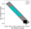 |
Fig. 1. Spatial distribution of the morphological data available in EGS field. Data from ACS-GC (Griffith et al. 2012), CANDELS (Brammer et al. 2012), and the OTELO survey (Bongiovanni et al. 2019), are shown in gray, cyan, and black, respectively. |
This paper is organised as follows. In Sect. 2, we describe the data used in this work. In Sect. 3, we present the description of the method used in this work. Section 4 provides the sample selection process and quantitative comparison with Griffith et al. (2012). In Sect. 5, we analyse the results of our fitting process and compare it to the ET and LT classification based on SED fitting. Furthermore, we analyse the MSR and compare it with previous works (Sect. 5.1). In Sect. 6, we provide a discussion of (i) the results of our morphological analysis using the (u − r) and compared it to the work of Strateva et al. (2001), as well as (ii) a discussion of the MSR found in this work and median size evolution for a given stellar mass since z = 2. In Sects. 7 and 8, we present a description of the morphological catalogue and our conclusions, respectively. When necessary we adopt the cosmology with ΩΛ = 0.69, Ωm = 0.31, and H0 = 67.8 km s−1 Mpc−1 from Planck Collaboration XIII (2016).
2. Data
2.1. The OTELO survey
The OTELO survey is based on the red tunable filters (RTF) images of the OSIRIS (Cepa et al. 2003) instrument at Gran Telescopio Canarias. A total of 36 RTF tomography slices were obtained. These slices were uniformly distributed in the spectral range between 9070 Å and 9280 Å, centered at 9175 Å. Following their reduction and alignment, the co-addition of these slices provide a detection image OTELOdeep, from which a total of 11 273 raw detections were extracted. The OTELOdeep photometry was complemented with archival data that was reprocessed, and PSF-matched to the OTELO’s resolution (pixel scale of 0.254″ px−1), available in EGS. Altogether, these data allowed to build the OTELO photometric catalogue2. Among the reprocessed archival data to OTELO pixel resolution are the images from HST-ACS (F606W and F814W) and from the Canada-France-Hawaii Telescope Legacy Survey (CFHTLS3; in u′, g′, r′, i′, z′ filters). Furthermore, the CFHTLS D3-25 i′-band source catalogue was used as the OTELO’s astrometric reference. The OTELO photometric catalogue was used to estimate photometric redshift zphot with LePhare code (Arnouts et al. 1999; Ilbert et al. 2006). Each photometric redshift solution obtained with LePhare code is associated with a specific galaxy template, which corresponds to a particular galaxy type. Templates used in this work are the following: four Hubble-type templates (E, Sbc, Scd, Im) from Coleman et al. (1980) and six starburst galaxy templates from Kinney et al. (1996). For the purpose of this work we consider those sources with a best-fitted template of the Hubble type E as ET, while LT refers to the sources fitted with the remaining ones.
The stellar masses were estimated following the method from López-Sanjuan et al. (2019), using rest-frame synthetic magnitudes obtained from the templates described above. For further details on the stellar masses M* and physical size estimations used in this work, we refer to Nadolny et al. (2020). We refer to the data-products described in this section as low-resolution (or low-res) because these were obtained on the basis of the RTF images with pixel scale of 0.254″ px−1. On the other hand, the morphological parameters were obtained from the original high-resolution HST-ACS images with pixel scale of 0.03″ px−1.
2.2. High-resolution Hubble Space Telescope data
The morphological catalogue is based on high-resolution images from HST-ACS F606W and F814W filters (hereafter V- and I-band, respectively). A total of 11 (overlapping with the OTELO survey field) HST-ACS tiles were retrieved from All-sky Extended Groth Strip International Survey (AEGIS) database4 in its native pixel scale of 0.03 arcsec px−1 and average resolution of ∼0.15 arcsec. This high-resolution data were acquired in HST Cycle 13 GO program 10134 (PI: M. Davis). In short, the HST-ACS images were already processed with standard ACS pipe-line (including bias subtraction, gain, and flat-field correction) and a python-based multi-drizzle package (Koekemoer et al. 2003) was applied to combine all exposures in one tile (including registration, median image creation, the identification and removal of cosmic rays).
In this study, we aim to complement the OTELO survey with the morphological analysis, thus we have to align the HST-ACS images to the same reference catalogue as used in the OTELO survey, that is, to the CFHTLS D3-25 i′-band source catalogue. This catalogue have an internal root mean square (RMS) astrometric error of 0.064 and 0.063 arcsec in equatorial coordinates5. An astrometry correction is necessary not only to provide homogeneous celestial coordinates of objects detected on the OTELOdeep image and its counterparts from high-resolution data, but also in our further analysis of morphological parameters. The initial astrometric offset between all of the 11 tiles used and CFHTLS catalogue were found to be different. Thus, we decided to provide a homogeneous astrometric correction for each of the tiles separately to the CFHTLS D3-25 i′-band catalogue before proceeding to the mosaic assembly.
The selection of the objects suitable for astrometry correction is important because we are matching low-resolution CFHTLS catalog (resolution ∼0.6 arcsec with pixel scale of 0.186 arcsec px−1) with high-resolution HST-ACS data (with resolution of ∼0.15 arcsec and pixel scale of 0.03 arcsec px−1). This selection was based on (i) CFHTLS i′-band magnitude (≤24.5), (ii) SExtractor (Bertin & Arnouts 1996) parameters CLASS_STAR ≥ 0.9 (for both images: HST I-band and CFHTLS i′-band), and (iii) FLAG = 0 for only high-resolution data. Furthermore, from these we selected visually a total of ∼370 point-like, isolated, and uniformly distributed on the OTELO’s field sources (∼33 objects per HST tile) as a final astrometric reference catalogue.
The astrometric reference catalogue was cross-matched with a source catalogue, which corresponds to each individual HST I-band tiles using IRAF ccxymatch task. The astrometric solution was obtained using IRAF ccmap third-order polynomial geometry with standard TNG projection. The accuracies of our astrometric solution in standard coordinates ξI and ηI are: 0.016 and 0.013 arcsec, respectively. This gives us off-set of 0.021 for the whole set of HST I-band tiles – namely, sub-pixel accuracy in high-resolution HST data with respect to CFHTLS D3-25 i′-band catalogue. The registration process of HST V-band images was based on the already aligned I-band data. The internal (i.e. between HST V- and I-band images) astrometric off-set is 0.002 arcsec.
The final mosaic of scientific and weight (inverse variance) images was obtained with SWarp6 software (Bertin et al. 2002). The mosaic was trimmed to the field of OTELOdeep image with additional ∼3 arcsec per side in order to provide morphological analysis of the objects which are on the border of the OTELO field of view.
3. Methods
3.1. Parametric classification
In this work, we used the GALAPAGOS2 software7 (Häußler et al. 2013), which, in turn, employs the applications SExtractor and GALFIT (Peng et al. 2002; in this case its new, multi-wavelength version GALFIT-M) to detect and to fit a single-Sérsic profile to each source, respectively. We chosen this parametric method due to its fully automatic operation: it detects, prepares initial values, runs GALFIT-M, reads-out the result for each source, and prepares a final catalogue. Furthermore, it handles the issues of neighbouring sources and sky background estimation in an accurate and efficient way (Häußler et al. 2013). However, one of the most important characteristic is that GALFIT-M fits simultaneously the selected model to all given bands using a chosen Chebyshev polynomial function. In this work, we used two photometric bands that increase the number of analysed sources and the accuracy of the parameter fitted to sources (especially with low S/N ratio) as compared with Griffith et al. (2012). For more, see Sect. 4.3 (also see simulations in Häußler et al. 2013, their Sect. 2).
We used the HST-ACS I-band images for source detection in the SExtractor dual mode, as implemented in GALAPAGOS2. Furthermore, following Rix et al. (2004), so called high-dynamical range (HDR) is used in order to maximise the source detection in two separate SExtractor runs with different parameter configurations. The first one (hot run), is optimized to detect faint sources, while the second one (cold run) is optimized to detect bright sources. In Table 1, we show the values of relevant parameters associated to hot and cold run. Since OTELO goes deeper in magnitude than ACS-GC catalogue, we decided to push the source detection in the faint end, thus, the SExtractor parameters were selected via trial and errors. After the hot and cold runs, GALAPAGOS2 takes care of matching both catalogues in such a way that hot detections inside a defined ellipse of a cold detection are not included (see Fig. 4 from Rix et al. 2004). We set the following GALFIT-M constraint values (the same as in Häußler et al. 2013): (1) position of the object that is to lie within the image cutout (hard-coded into GALFIT-M); (2) Sérsic index: 0.2 < n < 8; (3) effective radius: 0.3 < re, GF < 400 [px]; GF stands for the GALFIT-M output; (4) modeled magnitude: 0 < magGF < 40. Furthermore maginput − 5 < magGF < maginput + 5, where maginput is the input magnitude MAG_BEST from SExtractor and magGF is the output magnitude fitted with GALFIT-M; (5) axis ratio: 0.0001 ≤ Q ≤ 1, even if limits 0 ≤ Q ≤ 1 are hard-coded in GALFIT-M (based on the recommendation given by Häussler et al. 2007); (6) position angle: −180° < PA < 180° (hard-coded into GALFIT-M).
Main configuration parameters used in SExtractor HDR run.
Most of the input parameters in the configuration file were set to the default values, except for the parameters linked with the data used (pixel size, zero-points, exposure time, etc.). During the GALFIT-M fitting we fixed the center position of source to the X_IMAGE and Y_IMAGE I-band position, while linear Chebyshev polynomial function is used to fit magnitudes, effective radius re, and Sérsic index n over both HST-ACS bands used. In Sect. 5, the results obtained from the parametric method described above are compared with the LT and ET classification based on the best SED-fitting templates provided by the LePhare code (Sect. 2.1).
3.2. SExtractor derived parameters
A separate SExtractor run was executed to fully explore the high-resolution HST-ACS images. In this run SExtractor was fed with the same setup parameters (Table 1) and carried out in the same dual-HDR mode as in GALAPAGOS2. This assure the exact correspondence of sources detected in GALAPAGOS2 and this separated run. As the output we obtained, for each band used in this work, observed magnitudes (MAG_AUTO), flux radii (FLUX_RADIUS) corresponding to radii containing 20, 30, 50, 80, and 90% of the flux (used to derive the concentration index). We decided to perform this run because the output SExtractor catalogue from GALAPAGOS2 provide the parameter only for the detection band.
4. Sample selection
As established above, the goal of this work is to assign a morphological classification to the largest possible number of the OTELO survey sources detected in the OTELOdeep image. Since the OTELOdeep has lower spatial resolution than HST-ACS data used to provide the morphological catalogue, a careful match between both is needed. In the first part of this section, we describe the ‘cleaning’ process of the morphological GALAPAGOS2 catalogue obtained from analysis of the HST-ACS data, while in the second part, we explain the match and further selection of the galaxies, which are analysed in subsequent sections.
4.1. GALAPAGOS2 catalogue
Using the SExtractor dual HDR mode, we obtained 10 591 raw detections from the HST-I band. A total of 1778 (17%) raw detections were visually determined to be not real objects. Such high percentage is due to the fact that: (i) the final mosaic of HST-ACS images (Sect. 2.2) still shows imperfections and artifacts, especially on the borders of individual images; (ii) the SExtractor parameters were adjusted (via trial and error) to extract the maximum number of real sources, which on the other hand, increases detection of spurious sources. If our visual inspection omitted some of these bad detections, these were removed in the catalogue cleaning process, which is described in what follows. The list of coordinates of these artifacts was passed to GALAPAGOS2 in order to omit them in the fitting process.
A total of 8812 (out of 8813) sources were successfully fitted by GALAPAGOS2 that is, GALFIT-M does not crush, or does not exceed the time-limit for fitting process. We refer to this successfully fitted sources as G2 sample. The high rate of the successful fits is attributed to the visual inspection of the raw detections. The G2 sample, however, still contains sources for which one or more of the fitted parameters hit the constraint value (listed in Sect. 3.1) in one or both HST-ACS filters, thus, these results are not necessarily meaningful. Using criteria from Häußler et al. (2013, their Sect. 4.2) we identify sources characterised by these not necessarily meaningful results and we do not include them in the further analysis. Here, we list all the used criteria applied to both bands: (1) 0 < magGF < 40; (2) 0.205 < n < 7.95; (3) 0.301 < re < 399; (4) 0.001 < Q ≤ 1; (5) FLAG_GALFIT = 2. We omit the criterion (vi) from Häußler et al. (2013) due to our own star selection described in Bongiovanni et al. (2019). Applying those criteria we obtained a sample of 6780 sources with meaningful, or ‘good’ results (i.e. 77% of G2 sample, similarly as what is reported in Häußler et al. 2013). The cleaning process of the morphological catalogue, which involves removing results that are not meaningful for our study guarantees quality results in the following analysis. As shown in Fig. 2, this process removes the faint end of the G2 sample. The 50% magnitude completeness drop from ∼26.2 to ∼25.9 [AB] for the ‘good’ sample. Going forward, we use the G2 ‘good’ sample in subsequent sample selections.
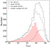 |
Fig. 2. Magnitude completeness. Continuous and dot-dash histograms in black represent the G2 and the ‘good’ samples, respectively. Dashed histogram in black shows the distribution of the sources removed from the G2 sample after the cleaning-out process (see Sect. 4.1). Red histogram shows the distribution of the morphological sample (see Sect. 4.2). Magnitudes indicated in the legend are 50% completeness magnitudes for each sample. |
4.2. Matching the GALAPAGOS2 and OTELO catalogues
We want to stress the importance of a reliable match between the results of the analysis of high-resolution HST-ACS images using GALAPAGOS2 and data from the OTELO catalogue, which are based on the low-resolution ground-based observations (photometry, photometric redshift, SED templates, ET-LT classification, and stellar masses, to name the relevant parameters used in this work). If we want to use any information derived from low-resolution data, we need to assure an exact correspondence between the sources coming from the high-resolution data. Due to the difference in spatial resolution, each source of the OTELO catalogue would admit one or multiple matches to the G2 sample. Hence, we checked the occurrence of one or more sources from G2 ‘good’ sample inside of the OTELOdeep detection ellipse (see example of multiple match in Fig. 3; ellipses were calculated using SExtractor parameters: A_IMAGE × KRON_RADIUS in arcsec). In this match, we got 5338 out of 6780 sources from the G2 ‘good’ sample. At this point, we removed objects which were classified as preliminary star candidates in the OTELO field (see Sect. 6.1 in Bongiovanni et al. 2019), which gives the total number of 5263 sources. Among these, there are 2780 individual (i.e. there is one source from G2 sample inside OTELO ellipse) matches between G2 sample and OTELO catalogue, while remaining 2483 sources are matched to 1295 OTELO sources, that is, there is more than one source inside OTELO ellipse (e.g., Fig. 3), and we refer to these as multiple matches. For each multiple match, we selected one source that is the closest to the OTELO catalogued position (usually the brightest counterpart), and we refer to these as multiple main. A total of 1108 multiple main sources were selected. A good example of multiple main is the central source, shown in the right panel of Fig. 3. This is a orthodox way of selecting a fairly clean sample in order to use data obtained from low-resolution OTELO data-products such as zphot, ET-LT classification, or stellar masses.
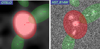 |
Fig. 3. Example of a multiple source with central multiple main objects (these images are available in our web-based graphic user interface). Left: low-resolution OTELOdeep image. Right: HST I-band high-resolution image. Ellipses in red (object in question) and green (neighbouring sources) show Kron ellipses from OTELOdeep image for individual OTELO sources. The red ellipse shows the Kron ellipse corresponding to the source id:2146, inside which two additional sources (or well defined parts of a single galaxy) are visible. This particular source has three matched sources from HST image. |
The visual inspection of the removed sources during the matching and cleaning out process reveals that these are, in many cases, point-like or very compact sources (possibly QSO), followed by those cases where interaction or merging sources are visible. There are also instances of sources which were excessively deblended by SExtractor (i.e. well-resolved galaxies with more than one visible part).
In Fig. 4, we show the difference of the output GALFIT-M model magnitude (IGF) and the input high-resolution I-band HST photometry (IGF − Iinput), as well as the low-resolution photometric data of the PSF-matched HST-ACS I-band from OTELO catalogue (IGF − Ilow − res.). This figure illustrates the importance of the match and selection process described above. This figure shows individual (green squares) together with multiple matches (red up-triangles) in the left column, while multiple (red left-triangles) and selected multiple main (blue squares) sources are on the right side. Considering the upper-left panel, we can clearly see that for individual sources, GALFIT-M returns expected values. The dispersion (upper-left panel, green squares) of the magnitudes towards brighter-output GALFIT-M magnitudes is expected due to the integration of the single-Sérsic model to infinity (e.g., Häussler et al. 2007; Häußler et al. 2013). While multiple main (upper-right panel, blue squares) behave in a similar way, their matched group members show larger dispersion. This is even more evident in the case of the low-resolution photometry (bottom row). Thus, even if, on one hand, we introduce bias in our sample selection, on the other hand, we guarantee the correspondence of the parameters from low-resolution data-base to the counterparts in high-resolution data.
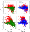 |
Fig. 4. Magnitude comparison between low- and high-resolution data. Red up- and left-triangles show multiple sources, green squares show individual sources, while blue squares shows multiple main sources. Top row: comparison of HST-ACS input and GALFIT-M output I-band magnitudes. Bottom row: same comparison as in top row, but instead of input high-resolution photometry we plot low-resolution HST-ACS-F814W photometry from OTELO catalogue. Lines represent the 25th and 75th percentile of the colour distribution per magnitude bin: light green dot-dashed – individual; dark red dashed – multiples; light blue dot-dashed – multiple main. See text for details on the samples selection (Sect. 4). |
On the basis of the source matching scheme described above, we focus on the meaningful results of the sources labeled as individual (2780) and multiple main sources (1108). This gives 3888 sources from which 3658 have any zphot solution from the OTELO catalogue while 2995 have zphot in the range 0 ≤ zphot ≤ 2 (hereafter morphological sample). Figure 5 shows the redshift distribution of the morphological sample, with LT (2873) and ET (122) sources up to zphot = 2. The peaks of distribution correspond to redshifts at which the OTELO survey sees specific emission lines, for example, zphot ∼ 0.35, 0.8, and 1.75 for Hα, [O III] and [Ne VI], respectively. We are aware of the possible misclassification of LT and ET using SED templates. However, de Diego et al. (2020) showed that less than 2% are misclassified using dense neural networks for the subset of the data used in this work (see their Sect. 3.1.4). Thus, for the aims of this work, we consider the OTELO’s classification as correct.
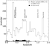 |
Fig. 5. Redshift distribution of the selected morphological sample (see text for details). Peaks in the distribution corresponds to specific emission lines, as seen in OTELO spectra range up to z = 2. Solid black line shows all sources in morphological sample, gray dot-dashed line shows LT galaxies, while black filled histogram shows ET galaxies. |
This restrictive selection process reduces dramatically the size of the final morphological sample (see Fig. 2). However, in order to use parameters derived in previous works (PSF photometry, zphot, templates classifications associated with zphot, stellar masses, and other OTELO-data products), this selection process is the most reasonable and responsible way to minimise possible biases due to the differences in the data used in the parameter estimation.
4.3. Comparison with ACS-GC catalogue
In this work, we used the same data as previously analysed by Griffith et al. (2012, ACS-GC catalogue), thus, we want to provide a quantitative comparison of the number of successfully analysed sources. The ACS-GC catalogue is based on the standard GALFIT version, which treats all bands separately. On the other hand, the multi-wavelength version GALFIT-M, implemented in GALAPAGOS2 and used in this work, allows us to simultaneously fit the data in all given bands using a linear Chebyshev polynomial. This multi-wavelength version of GALFIT has been shown to be more robust for the low-S/N bands (Häußler et al. 2013). For the purpose of this comparison, we used a common sample composed of the matched sources from ACS-GC and our G2 sample (with 8812 objects, see Sect. 4.1 for G2 sample definition). A total of 4724 sources were matched, and these constitute the common sample. The remaining 4088 sources from our G2 sample have no counterpart in ACS-GC (OTELO-only sample). The model-based I-band magnitude for both, the common sample, and the OTELO-only sample are shown in Fig. 6. Since the OTELO-only sample may still contain results that are not meaningful for our study, we additionally show the magnitude distribution for each sub-sample which corresponds to the morphological sample defined in Sect. 4.2. From these sub-samples, a total of 3015 sources were found in common (median I-band mag. = 24.4), while the remaining 873 were detected only in the OTELO catalogue (median I-band mag = 26). We recovered a significant number of robust sources not presented in previous works, which fall into the faint end of the magnitude distribution (∼1.5 mag fainter).
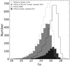 |
Fig. 6. Magnitude comparison with Griffith et al. (2012). Step histogram in gray (dot-dashed line) show common sample, while step histogram (continuous line) show remaining OTELO sources with no matched counterpart from ACS-GC (i.e. only found in OTELO). Filled gray and black histograms correspond to the morphological sample (see Sect. 4.2) from common sample and without counterpart from ACS-GC (i.e. only found in OTELO), respectively. Numbers in the legend indicate the number of sources in the particular sub-sample. |
Regarding the common sample (4724 sources), in Fig. 7 we show comparison of model-based I-band results for magnitudes IGF, Sérsic index nI, and effective radius re, I. In order to make our comparison sensitive to S/N, we divided the common sample into four magnitude bins (IGF ≤ 24, 24 < IGF ≤ 25, 25 < IGF ≤ 26, and IGF > 26; colour-coded in all panels). The left panel shows the magnitude comparison and it is clear that both catalogues are in agreement. The middle and right panels represent the Sérsic index, nI, and effective radius, re, I for a direct comparison of both catalogues, ACS-GC and OTELO. In the middle panel, where nI is represented, we can notice that part of ACS-GC results is accumulated in three discrete values, that is, at nI = 0, around 0.2, and 8. These are the results for which GALFIT run into constraint values, and should not be considered as valid. While this is clearly visible for ACS-GC, much fewer sources are found at these constraint values among the OTELO results. The same is true for the effective radius, re, shown on the right panel, although less pronounced, as compared to the Sérsic index.
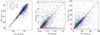 |
Fig. 7. Comparison of the results from this work with those obtained by Griffith et al. (2012) for the common sample. From left to right: model-based I-band magnitude IGF, Sérsic index nI, and effective radius re, I. Sources corresponding to each magnitude bin are colour-coded, as shown in the legend on the left panel. Red dashed lines represent 1:1 relation. |
In Fig. 8, we show histograms for nI and re, I per magnitude bins. In these histograms, we include sources from the common sample after applying the criteria 2 and 3 listed in Sect. 4.1 (i.e. 0.205 < nI < 7.95, and 0.301 < re, I < 399, thus removing sources with results that hit constraint values) for both catalogues. We indicate the difference of the sources in OTELO and ACS-GC for each parameter and bin (numbers between brackets) after applying the aforementioned criteria. As can be seen, for both parameters and all magnitude bins, OTELO has substantially more sources with meaningful results. The greatest difference is observed in the faintest bin, thus confirming that the multi-wavelength version of GALFIT used in this work is more robust, especially in the low S/N regime. Similar results are obtained for the remaining parameters, as well as for the V-band.
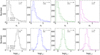 |
Fig. 8. Comparison of the results from this work with those obtained by Griffith et al. (2012). Top row: contains a comparison of the Sérsic index nI distributions, while the bottom row represents the logarithm of effective radius re, I. Each panel show a comparison for each magnitude bin indicated in the top-right corner. Numbers between brackets show the number of sources recovered in this work. |
5. Morphology analysis
Among the data returned by GALAPAGOS2 there are model-based parameters like magnitudes (VGF, IGF), Sérsic indices (n), and effective radii (re, containing 50% of the model flux) for each input filter, that is, HST-ACS I- and V-band. The analysis also includes the parameters obtained from the separate SExtractor run, as described in Sect. 3.2 (e.g., concentration index), as well as stellar masses, M*, from Nadolny et al. (2020).
Figure 9 shows the results of a linear discriminant analysis of model-based (VGF − IGF) and observed (u − r) colours performed to find the most accurate ET-LT separation. We found cuts of 1.7 and 2.5 to be the most accurate for (VGF − IGF) and (u − r), respectively. Using these limits, we found ET completeness and contamination of 39% and 63% for (VGF − IGF), and 62% and 35% for (u − r), respectively. The small spectral separation of the filters used to calculate the (VGF − IGF) colour translates into the relatively poor separation of ET from LT galaxies, with a higher contamination of LT in the expected region for ET. The (u − r) colour with larger wavelength separation, gives better results in terms of completeness and contamination. This shows that (u − r) is more adequate for ET-LT separation. The (u − r) colour cut found in this work is higher than that reported by Strateva et al. (2001) and we attribute this with the redshift range of our sample.
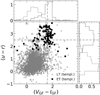 |
Fig. 9. Comparison between (VGF − IGF) and (u − r) colours. Triangles and solid lines in gray represent LT, squares and dashed lines in black correspond to ET galaxies. Top and right-hand: density histograms correspond to (VGF − IGF) and (u − r), respectively. Dot-dashed lines show the results of linear discriminant analysis of both colours with (VGF − IGF) = 1.7 and (u − r) = 2.5. |
The high completeness (> 97%) of LT in blue cloud is likely due to the selection process, where we cleared out the morphological sample from possible QSO or AGN and mergers or interacting galaxies, as described in Sect. 4.1. In order to carry out a second check, we used the criteria from Schawinski et al. (2014, their Eqs. (1) and (2)) to separate blue cloud, green valley, and red sequence galaxies. We found that ∼8% of our LT galaxies are in their red sequence as compared with 7% in their work (see their Table 1).
The bottom-left panel of Fig. 10 shows the Sérsic index distribution as a function of (u − r) colour. The overall Sérsic indices fall in the expected ranges of values for ET and LT galaxies (top-left histogram). The median values of nI index are 1.3 ± 0.6 and 3.0 ± 0.9 for LT and ET, respectively. Uncertainties cited in this section are median absolute deviations. The increase of n from LT to ET is expected, since LT are disc-dominated (described with lower Sérsic index of n ∼ 1) and ET are bulge-dominated (i.e. n ≳ 4) galaxies. A very similar trend is observed for nV (measured on V-band) with median values of 1.1 ± 0.6 and 3.0 ± 1.2 for LT and ET, respectively. The V-band results are not shown for the sake of clarity. As can be seen in the same panel of Fig. 10, there are two well-defined regions occupied by red & high-n ET galaxies [(u − r) > 2.3 and log n > 0.4] and blue & low-n LT galaxies [(u − r) < 2.3 and log n < 0.4]. We found a ET completeness in the red & high-n zone of 59%, with a contamination of 30%. The completeness (and contamination) provided by this method according to Vika et al. (2015) is of 63% (53%) for their artificially redshifted sample (see their Table 1). In the same panel of Fig. 10, we show the results of the linear discriminant analysis from de Diego et al. (2020). Using this discriminant for the morphological sample, we found 98% and 66% of completeness for LT and ET, respectively.
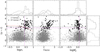 |
Fig. 10. Observed (u − r) colour as a function of morphological parameters. From left to right: Sérsic index, nI, concentration index, c90/50, and wavelength-dependent ratio of Sérsic indices |


The concentration index c90/50, defined as ratio of SExtractorI-band flux radius containing 90% and 50% of the flux, is shown in the middle panel of Fig. 10. The median values of I-band c90/50 are 1.9 ± 0.2 and 2.4 ± 0.2 for LT and ET, respectively. Again, very similar median values are observed for V-band c90/50 with 1.9 ± 0.2 and 2.3 ± 0.2 for LT and ET. As shown in previous works (e.g., Strateva et al. 2001), this parameter does not provide a good separation of ET-LT and it can only yield a crude classification.
The last parameter in Fig. 10 (third panel) shows the ratio of Sérsic indices in both HST bands  /nV, as defined by Vika et al. (2015). This parameter, together with a colour term, is shown to be sensitive to the internal structure. Median values of
  for LT and ET are 1.1 ± 0.4 and 1.0 ± 0.2, respectively. This indicates that the ET sub-sample is well defined around
  . This is an expected result because of the very nature of red ET galaxies, which show less variation of the Sérsic profile with wavelength (e.g., Vulcani et al. 2014). Using cuts of
  and (u − r) > 2.3, Vika et al. (2015) found 70% of completeness and 50% of contamination for ET galaxies. Here, we report 60% of ET completeness with 42% of LT contamination using the same cuts in
  and (u − r).
5.1. Testing the mass–size relation
Using stellar masses, M*, and physical sizes estimated using model-based flux radius, re, we can study the mass–size relation (MSR). In order to probe if there are any signs of evolution in the MSR since z = 2, we divided our sample into three redshift bins or volumes (vol1: z < 0.5, vol2: 0.5 ≤ z < 1, and vol3: 1 ≤ z < 2). For each bin and for each morphological type, we fit a single power law of the form:
 (2)
(2)
The parameters of the best-fit functions for each cosmic volume, as well as median redshifts, are given in Table 2. These functions are represented in Fig. 11. As can be seen, the slope of the relation fitted in this process do not vary significantly between different redshift bins for a given morphological type (the black lines in the middle and right panel in Fig. 11 show the fits from the first redshift bin). It is noticeable that, on one hand OTELO miss the high-mass end (> 1011 M⊙) of the LT and ET galaxies, while on the other hand, there is also a low store of statistics with regard to the ET galaxies in the last redshift bin (resulting in high errors in the best-fit power law; see Table 2).
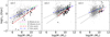 |
Fig. 11. Mass–size relation. Each panel correspond to selected cosmic volumes: z < 0.5, vol2: 0.5 ≤ z < 1, and vol3: 1 ≤ z < 2. Gray triangles and black squares show LT and ET galaxies, respectively. Dot-dashed blue and dashed red lines show power–law fits for LT and ET data, respectively, according to Eq. (2). The best-fit parameters are given in Table 2. Gray dot-dashed, and dashed lines in the middle and right panels show the fits for LT and ET obtained for the first cosmic volume (vol1). Dot-dashed green and dashed magenta lines represent LT (SF) and ET (Q) MSR from Mowla et al. (2019). |
Results of the power law fitting of the MSR.
The OTELO survey was designed to recover the low-mass end of the field galaxy population. Indeed, in our MSR, we can see that it extends towards lower stellar masses, if compared with previous works. Thus, in all panels of Fig. 11 we additionally represent the fits from Mowla et al. (2019) for star-forming (LT) and quiescent (ET) for the same redshift bins. Their separation onto star-forming and quiescent galaxies is based on U, V, and J rest-frame bands. For the purpose of the comparison, presented in what follows, this selection is compatible with our ET-LT separation (van der Wel et al. 2014). Our MSR for LT galaxies is consistent with those given by Mowla et al. (2019), even taking into account the differences in the mass range studied in both works. However, the slope obtained by these authors in the case of ET galaxies is stepper than the fitted in this work for all redshift bins, with the largest difference in the last volume 1 ≤ z < 2 (0.73 and 0.56, in Mowla et al. 2019 and in this work, respectively). This difference mainly obeys to the fact that the galaxies studied in Mowla et al. (2019) are massive log M*/M⊙ > 11.3, complemented with galaxies from van der Wel et al. (2014, 3D-HST+CANDELS). Precisely, this addendum contains a great part of the ET galaxies of the resulting sample in the last redshift bin studied in their work. Since both works, van der Wel et al. (2014) and Mowla et al. (2019) are consistent, we decided to only keep the fits from the latter.
It is worthwhile noting that due to the limited OTELO’s field of view (∼56 arcmin2), the co-moving volume surveyed is relatively small if compared with broadly known extragalactic surveys (e.g., SDSS, COSMOS, CANDELS). This fact may introduce a bias towards the detection of sources with lower masses, thus losing the high-mass end. For instance, if the results of the zCOSMOS survey are scaled to the sky area explored by OTELO, and using the same selection criteria given by López-Sanjuan et al. (2012, i.e. 0.1 < z < 1.1, log M*/M⊙ > 11 and OTELOdeep < 24), we should find 11 sources in the census of the OTELO survey. However, following the selection process described in Sect. 4, we are left with only four sources. Hence, it is necessary to stress that we lose ∼60% of the high-mass end as a result of the limited sky covering of our survey.
In Fig. 12, we show ET and LT galaxies analysed in this work without separation onto redshift bins. In this figure, we show the power–law fits to the whole ET and LT samples (tabulated in the bottom part of Table 2), as well as results from Lange et al. (2015, their Tables 2 and 3, i-band fits), where the local galaxy sample was studied (0.01 < z < 0.1, log M*/M⊙ ∼ 7.5 − 11). The MSR for ET and LT populations of OTELO are consistent with the low-redshift relation. In order to test the effects of the selected stellar mass range when comparing our results with previous studies, we limited our sample to the lower limits given in Shen et al. (2003). These limits in log M*/M⊙ are 10.1 and 8.8 for ET and LT galaxies, respectively. Both limits correspond to median mass values of ET and LT samples studied in this work (i.e. by removing considerable part of our sample). Even so, using these mass-limited samples, we found a good agreement between our fit and the results of Shen et al. (2003). For the sake of clarity, we do not include these results in Fig. 12. In the top panel of the same figure, we show the distribution of stellar masses for ET and LT galaxies. It is noticeable that both populations dominate in different mass regimes, with median values of log M*/M⊙ ∼ 8.8 and 10.12 for LT and ET galaxies, respectively. On the other hand, as can be seen on the right panel of Fig. 12, both galaxy populations occupy the similar range of physical sizes. In Sect. 6, we present more detailed discussion on possible median size evolution in the re − z space.
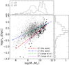 |
Fig. 12. Mass–size relation. Gray triangles and black squares show LT and ET galaxies, respectively. Dot-dashed blue and dashed red lines show linear fits for LT and ET data, respectively. Thin dot-dashed green and dashed magenta lines represent LT and ET MSR from Lange et al. (2015). Top and right panels: density histograms of stellar mass and size, respectively. The results of the fitted power law parameters are given at the bottom of Table 2. |
5.2. Errors
As described in Peng et al. (2010), the formal uncertainties derived in GALFIT-M are only the lower estimates. After extensive simulations and tests of this software, Häussler et al. (2007) provided estimates of uncertainties based on the comparison of input and output values as a function of surface brightness. In Fig. 13, we show the errors from Häussler et al. (2007) and nominal errors from GALFIT-M from this study as a function of the surface brightness (defined as in Häussler et al. 2007), given by:
![Mathematical equation: $$ \begin{aligned} \mu _{\rm output} = {\mathrm{mag} + 2.5 \log [2(b/a)\,\pi \,r_{\rm e}^{2}]}, \end{aligned} $$](/articles/aa/full_html/2021/03/aa37861-20/aa37861-20-eq10.gif) (3)
(3)
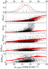 |
Fig. 13. Errors of given parameter as a function of surface brightness μoutput. Black dots show the outcome from this work and the red dots show data for selected (f1 = 1) galaxies from Häussler et al. (2007). Top panels: density distribution of μoutput with median values marked as red dashed-lines (22.3) and black dot-dashed lines (23.04). |
where mag is the I-band magnitude, b/a the axis ratio, and re the half-light radius in arcseconds. The μoutput is calculated using the output GALFIT-M parameters. We note that even the nominal error values are the lower estimates, as it is clearly seen that these behave as expected – the errors increase with surface brightness for all parameters (even if this is not so evident for n, Q, and PA). This is also seen if the errors are represented as a function of Iinput (however, we do not show this relation here). We report the nominal values of the errors with the indication that these are lower-bound estimates (at least for bright objects) since the total error budget would require performing simulations as in Häussler et al. (2007), which is beyond the scope of this work.
6. Discussion
Strateva et al. (2001) demonstrated that a (u − r) = 2.22 colour-cut separation can be useful for a broad segregation of ET from LT. They used a sample with more than 140 000 galaxies from the SDSS survey down to magnitude g = 21 and z < 0.4. Even though this particular method does not directly use the parameters derived in this work, it is interesting to test its performance using the OTELO catalogue. This method uses parameters that are relatively easy to obtain, namely, the observed magnitudes in the g, r, and u bands, which are available also in the OTELO catalogue. Figure 15 shows how this method is able to separate sources in the morphological sample up to zphot = 2. Nearly 81% (97%) of ET (LT) from the morphological sample are correctly separated, namely, with (u − r) ≥ 2.22 (< 2.22). The reliability (defined as in Strateva et al. 2001) of ET (LT) selection for this method is of 54% (99%). As compared to values from Strateva et al. (2001), their ET (LT) completeness and reliability are 98% (72%) and 83% (96%) for the spectroscopic sample and 80% (66%) and 62% (83%) for visually classified galaxies, respectively (see their Tables 2 and 3). Although the completeness of our ET selection using this method decreases slightly, our sample extends to a much higher redshift and is deeper in magnitude than both samples presented in Strateva et al. (2001). Despite this, an appropriate (u − r) colour-cut separation could be used as a fair proxy to a ET-LT segregation in OTELO data.
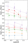 |
Fig. 14. Median size evolution with redshift, the re − z relation. Median sizes are shown for fixed stellar mass bins centered at log M*/M⊙ = 8, 9, 10, 10.5, and 11 with colours indicated in the figure (bin width of 0.5 dex). We note that only three of the most massive bins are shown for ET for each volume (top panel). Filled symbols represent data from this work, while open markers shows data from Mowla et al. (2019), their Table 3 (including errors). Our error bars represent the median absolute deviation of the data in each bin. We plot median sizes for bins that have more than three sources. |
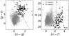 |
Fig. 15. ET-LT colour separation from Strateva et al. (2001) using data from this work. Gray triangles and black squares represents LT and ET galaxies classified via templates. Dot-dashed line represent (u − r) = 2.22. |
The stellar mass–size relations for ET and LT (Fig. 12) in our sample, regardless of the separation in redshift bins, are in agreement with the general trends at low redshift reported in the recent literature (Shen et al. 2003; Lange et al. 2015). According to these authors, and leaving aside the data scattering, the MSR for ET galaxies is steeper than the corresponding to LT, as confirmed in this work. Furthermore, the stellar mass distributions show a sort of bi-modality, with LT galaxies being less massive than ET sources (in our case, with median values of log M*/M⊙ = 8.8 and 10.12, respectively). Finally, according to the results given in Sect. 5 we cannot draw any conclusion about the possible evolution of the MSR in both types, considering stellar-mass range studied (Fig. 12). Recent studies of the MSR in similar redshift range as studied in this work (e.g., van der Wel et al. 2014; Roy et al. 2018; Mowla et al. 2019, and references therein) point out to a median size evolution of galaxies with redshift (re − z). In particular, Mowla et al. (2019) used I-band HST-ACS images to quantify the re − z relation for COSMOS-DASH survey, that is, the same instrument and filter of the HST as in this work. The use of the same photometric band is especially important because of the claimed dependence of size on the wavelength at which the measurements are done (e.g., Kelvin et al. 2012). Since the MSR presented by Mowla et al. (2019) do not match stellar-mass ranges studied here, we compare the re − z for three fixed mass of log M*/M⊙ = 10, 10.5, and, 11 and, furthermore, including lower-mass bins of log M*/M⊙ = 8 and 9 for the LT galaxies from this work. In Fig. 14, we show the results of this comparison. In this figure, we only plotted median size values for bins where we have more than three objects (we note that for the ET most massive stellar-mass bin, we plotted only the intermediate redshift bin). This ensures a more robust comparison with previous works. Considering, the re − z relation for fixed stellar-mass of log M*/M⊙ = 10.5 (red lines and points in Fig. 14) for which OTELO have sufficient statistics in both morphological types, we can notice that our results are consistent with Mowla et al. (2019): ET galaxies present steeper median size evolution, as compared to LT population. Furthermore, we show the median size evolution for LT galaxies in the previously unexplored mass regime, namely, for log M*/M⊙ of 8, and 9. These are two mass bins where OTELO do have sufficient number of sources in all redshifts (between ∼50 and ∼450). We find very mild evolution of median size for these masses, which is compatible with the scenario of passive evolution for this type of galaxy (e.g., van der Wel et al. 2014; Mowla et al. 2019). Generally speaking, and taking into account the biases introduced in our selection process (under-representation of high-mass end), our results are in agreement with previous findings on MSR, as well as on the median size evolution re − z.
7. Morphological catalogue
Together with this work, we are making the morphological catalogue public, along with the aforementioned parameters. The catalogue can be retrieved from our website or from the CDS. Table 3 provides the description of parameters in the catalogue. The unique the OTELO object number idobj can be used to match results from this work with the OTELO catalogue. The catalogue presented in this work consists of the G2 sample (as defined in Sect. 4) with 8813 detections in HST-ACS I-band image, namely, all the sources with a successful fit from GALAPAGOS2 (not necessarily meaningful). The flag flag_good (=1) indicates the meaningful selection (6780). The derived parameters from GALAPAGOS2 were measured in both available bands, namely, V (F606W) and I (F814W) from HST-ACS. The morphological sample (studied in this work) can be easily recovered using 0 < z_phot < 2. These are sources with ‘good’ GALAPAGOS2 output parameters and with individual match to the OTELO catalogue (the closest in the case of multiple matches). For these sources, we include several parameters from the OTELO catalogue (unique OTELO id idobj, selected photometric redshift z_phot, and template associated with selected redshift; see Sect. 2.1) and the stellar mass estimation from Nadolny et al. (2020). The multiple matches can be identified by GroupID and GroupSize, however only the closest to the OTELO catalogue position is indicated, for sake of clarity. In Fig. 16 we show images from the fitting process with original, model, and residual images for several sources.
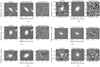 |
Fig. 16. Examples of LT (left column) and ET (right column) sources. For each source, we show (from left to right) the original HST-ACS-I band image, GALFIT-M model and residual image. LT and ET classification is obtained from SED fitting to the templates, as described in Sect. 2.1. (a) id: 1003. (b) id: 279. (c) id: 5691. (d) id: 6176. (e) id: 7249. (f) id: 10555. |
Column description of the morphological catalogue.
8. Conclusions
In this paper, we aim to present the morphological catalogue of 8813 sources detected in HST-ACS I-band in the framework of the OTELO survey. This catalogue contains the multi-wavelength morphological parameters of a single-Sérsic model fitted to HST-ACS V- and I-bands employing GALAPAGOS2, as well as stellar masses. The unique combination of this morphological and the OTELO catalogues provides a valuable tool for the study of different aspects of galaxy evolution.
Using OTELO’s ET-LT galaxy classification via templates, we examined some of the methods found in the literature using the derived parameters. A rigorous sample selection assures the exact correspondence of data from the OTELO catalogue to morphological parameters obtained from the high resolution images. We found great similarities in the results with regard to previous works of ET and LT separation in terms of the Sérsic index n, ratio of Sérsic index in I- and V-band  , and observed colour (u − r). Furthermore, we also tested an independent classification method which uses only the observed colours, described in Strateva et al. (2001). A general agreement was found despite its own reliability.
Due to the statistical similarities among the ET-LT separation using methods employed in the low-z Universe, we found no evidence of evolution for the studied parameters. This is also confirmed in the case of the MSR relation, which we found to closely follow the local MSR from Lange et al. (2015, z < 0.1), as shown in Fig. 12. We note, however, that our selection process does indeed bias the sample, and in the case of MSR, we lose a portion of the massive (log M*/M⊙ > 11) ET galaxies. This bias towards less massive galaxies in our sample is evident when comparing our results to the sample obtained with MSR of more massive (log M*/M⊙ > 11.3) sources at the same redshift bins (Mowla et al. 2019). In particular, the MSR for ET galaxies for the highest redshift bin is not sufficiently sampled, resulting in an offset of ∼0.4 dex in size. This is also reflected in the errors of the power–law parameters fitted for this particular sub-sample. We also investigated the median size evolution since z = 2, finding a good agreement with the recent study of Mowla et al. (2019): the median size of ET galaxies evolves more steeply than the median size of LT for a given stellar mass. In any case, these results corroborate the fact that our sample is composed of field galaxies. Thus, we are in the position to make comparisons between cluster versus field galaxies – which is to make up the scope of a future work. In this context, we will make use of the GLACE survey (Sánchez-Portal et al. 2015), whose design and purpose are very closely related to those of the OTELO survey.
Several scientific cases are under study by our team using this dataset. These are: a comparison of sources with and without emission lines detected in OTELO; using machine learning techniques to improve ET-LT separation through colour proxies, morphology, and redshift (e.g., using the catalogue from this work with OTELO photometry and redshift in de Diego et al. 2020); a comparison of cluster versus field galaxies; and, finally, a study of compact galaxies and ET galaxies with emission lines. The latter two are already in preparation.
Together with this paper, we provide a public morphological catalogue with 8813 entries as described in Sect. 7 and Table 3. The sources studied in this article, along with additional information (stellar masses, zphot, and morphological classification via templates) can be easily recovered from the catalogue.
For the extensive list of archival data included in the OTELO photometric catalogue we refer to Bongiovanni et al. (2019).
See “T0007: The Final CFHTLS Release” at http://terapix.iap.fr/cplt/T0007/doc/T0007-doc.pdf
Acknowledgments
This paper is dedicated to the memory of our dear friend and colleague Hector Castañeda, unfortunately died on 19 Nov. 2020. This work was supported by the project Evolution of Galaxies, of reference AYA2014-58861-C3-1-P and AYA2017-88007-C3-1-P, within the “Programa estatal de fomento de la investigación científica y técnica de excelencia del Plan Estatal de Investigación Científica y Técnica y de Innovación (2013-2016)” of the “Agencia Estatal de Investigación del Ministerio de Ciencia, Innovación y Universidades”, and co-financed by the FEDER “Fondo Europeo de Desarrollo Regional”. APG, RPM and MSP was supported by AYA2017-88007-C3-2-P. APG and MC are also supported by the Spanish State Research Agency grant MDM-2017-0737 (Unidad de Excelencia María de Maeztu CAB). JAD is grateful for the support from the UNAM-DGAPA-PASPA 2019 program, and the kind hospitality of the IAC. Based on observations made with the Gran Telescopio Canarias (GTC), installed in the Spanish Observatorio del Roque de los Muchachos of the Instituto de Astrofísica de Canarias, on the island of La Palma. This paper made use of the IAC Supercomputing facility HTCondor (http://research.cs.wisc.edu/htcondor/). This paper made use of the Wright (2006) cosmological calculator. Based on observations obtained with MegaPrime/MegaCam, a joint project of CFHT and CEA/IRFU, at the Canada-France-Hawaii Telescope (CFHT) which is operated by the National Research Council (NRC) of Canada, the Institut National des Science de l’Univers of the Centre National de la Recherche Scientifique (CNRS) of France, and the University of Hawaii. This work is based in part on data products produced at Terapix available at the Canadian Astronomy Data Centre as part of the Canada-France-Hawaii Telescope Legacy Survey, a collaborative project of NRC and CNRS. M.A.L.L. is a DARK-Carlsberg Foundation Fellow (Semper Ardens project CF15-0384). MP acknowledges financial financial support from the Ethiopian Space Science and Technology Institute (ESSTI) under the Ethiopian Ministry of Innovation and Technology (MInT), and of the Spanish MEC undergrant AYA2016-76682-C3-1-P and PID2019-106027GB-C41 and financial support from the State Agency for Research of the Spanish MCIU through the “Center of Excellence Severo Ochoa” award to the Instituto de Astrofísica de Andalucá (SEV-2017-0709).
References
- Abraham, R. G., Valdes, F., Yee, H. K. C., & van den Bergh, S. 1994, ApJ, 432, 75 [NASA ADS] [CrossRef] [Google Scholar]
- Abraham, R. G., van den Bergh, S., Glazebrook, K., et al. 1996, ApJS, 107, 1 [NASA ADS] [CrossRef] [Google Scholar]
- Abraham, R. G., van den Bergh, S., & Nair, P. 2003, ApJ, 588, 218 [NASA ADS] [CrossRef] [Google Scholar]
- Andrae, R., Jahnke, K., & Melchior, P. 2011b, MNRAS, 411, 385 [NASA ADS] [CrossRef] [Google Scholar]
- Andrae, R., Melchior, P., & Jahnke, K. 2011a, MNRAS, 417, 2465 [NASA ADS] [CrossRef] [Google Scholar]
- Arnouts, S., Cristiani, S., Moscardini, L., et al. 1999, MNRAS, 310, 540 [NASA ADS] [CrossRef] [Google Scholar]
- Baldry, I. K., Glazebrook, K., Brinkmann, J., et al. 2004, ApJ, 600, 681 [Google Scholar]
- Barden, M., Rix, H.-W., Somerville, R. S., et al. 2005, ApJ, 635, 959 [NASA ADS] [CrossRef] [Google Scholar]
- Barden, M., Häußler, B., Peng, C. Y., McIntosh, D. H., & Guo, Y. 2012, MNRAS, 422, 449 [NASA ADS] [CrossRef] [Google Scholar]
- Bershady, M. A., Jangren, A., & Conselice, C. J. 2000, AJ, 119, 2645 [NASA ADS] [CrossRef] [Google Scholar]
- Bertin, E., & Arnouts, S. 1996, A&AS, 117, 393 [NASA ADS] [CrossRef] [EDP Sciences] [Google Scholar]
- Bertin, E., Mellier, Y., Radovich, M., et al. 2002, in Astronomical Data Analysis Software and Systems XI, eds. D. A. Bohlender, D. Durand, & T. H. Handley, ASP Conf. Ser., 281, 228 [NASA ADS] [Google Scholar]
- Bongiovanni, Á., Ramón-Pérez, M., Pérez García, A. M., et al. 2019, A&A, 631, A9 [NASA ADS] [CrossRef] [EDP Sciences] [Google Scholar]
- Brammer, G. B., van Dokkum, P. G., Franx, M., et al. 2012, ApJS, 200, 13 [Google Scholar]
- Cepa, J., Aguiar-Gonzalez, M., Bland-Hawthorn, J., et al. 2003, in SPIE Conf. Ser., eds. M. Iye, & A. F. M. Moorwood, Proc. SPIE, 4841, 1739 [NASA ADS] [Google Scholar]
- Ciotti, L. 1991, A&A, 249, 99 [NASA ADS] [Google Scholar]
- Coleman, G. D., Wu, C.-C., & Weedman, D. W. 1980, ApJS, 43, 393 [NASA ADS] [CrossRef] [Google Scholar]
- Conselice, C. J., Bershady, M. A., & Jangren, A. 2000, ApJ, 529, 886 [NASA ADS] [CrossRef] [Google Scholar]
- de Diego, J. A., Nadolny, J., Bongiovanni, Á., et al. 2020, A&A, 638, A134 [NASA ADS] [CrossRef] [EDP Sciences] [Google Scholar]
- de Souza, R. E., Gadotti, D. A., & dos Anjos, S. 2004, ApJS, 153, 411 [NASA ADS] [CrossRef] [Google Scholar]
- de Vaucouleurs, G. 1959, Handb. Phys., 53, 275 [NASA ADS] [Google Scholar]
- Dressler, A., Faber, S. M., Burstein, D., et al. 1987, ApJ, 313, L37 [NASA ADS] [CrossRef] [Google Scholar]
- Freeman, K. C. 1970, ApJ, 160, 811 [Google Scholar]
- Graham, A. W., Driver, S. P., Petrosian, V., et al. 2005, AJ, 130, 1535 [NASA ADS] [CrossRef] [Google Scholar]
- Griffith, R. L., Cooper, M. C., Newman, J. A., et al. 2012, ApJS, 200, 9 [Google Scholar]
- Häussler, B., McIntosh, D. H., Barden, M., et al. 2007, ApJS, 172, 615 [NASA ADS] [CrossRef] [EDP Sciences] [Google Scholar]
- Häußler, B., Bamford, S. P., Vika, M., et al. 2013, MNRAS, 430, 330 [NASA ADS] [CrossRef] [Google Scholar]
- Hubble, E. P. 1925, ApJ, 62, 409 [NASA ADS] [CrossRef] [Google Scholar]
- Hubble, E. P. 1936, Realm of the Nebulae (New Haven: Yale University Press) [Google Scholar]
- Huertas-Company, M., Rouan, D., Tasca, L., Soucail, G., & Le Fèvre, O. 2008, A&A, 478, 971 [NASA ADS] [CrossRef] [EDP Sciences] [Google Scholar]
- Huertas-Company, M., Gravet, R., Cabrera-Vives, G., et al. 2015, ApJS, 221, 8 [NASA ADS] [CrossRef] [Google Scholar]
- Ilbert, O., Arnouts, S., McCracken, H. J., et al. 2006, A&A, 457, 841 [NASA ADS] [CrossRef] [EDP Sciences] [Google Scholar]
- Jiménez-Teja, Y., & Benítez, N. 2012, ApJ, 745, 150 [NASA ADS] [CrossRef] [Google Scholar]
- Kauffmann, G., Heckman, T. M., White, S. D. M., et al. 2003, MNRAS, 341, 54 [Google Scholar]
- Kelly, B. C., & McKay, T. A. 2005, AJ, 129, 1287 [NASA ADS] [CrossRef] [Google Scholar]
- Kelvin, L. S., Driver, S. P., Robotham, A. S. G., et al. 2012, MNRAS, 421, 1007 [NASA ADS] [CrossRef] [Google Scholar]
- Kinney, A. L., Calzetti, D., Bohlin, R. C., et al. 1996, ApJ, 467, 38 [NASA ADS] [CrossRef] [Google Scholar]
- Koekemoer, A. M., Fruchter, A. S., Hook, R. N., & Hack, W. 2003, in HST Calibration Workshop: Hubble after the Installation of the ACS and the NICMOS Cooling System, eds. S. Arribas, A. Koekemoer, & B. Whitmore, 337 [Google Scholar]
- Kormendy, J. 1977, ApJ, 218, 333 [NASA ADS] [CrossRef] [Google Scholar]
- Kormendy, J., & Bender, R. 1996, ApJ, 464, L119 [NASA ADS] [CrossRef] [Google Scholar]
- Krywult, J., Tasca, L. A. M., Pollo, A., et al. 2017, A&A, 598, A120 [NASA ADS] [CrossRef] [EDP Sciences] [Google Scholar]
- Kuchner, U., Ziegler, B., Verdugo, M., Bamford, S., & Häußler, B. 2017, A&A, 604, A54 [NASA ADS] [CrossRef] [EDP Sciences] [Google Scholar]
- Lange, R., Driver, S. P., Robotham, A. S. G., et al. 2015, MNRAS, 447, 2603 [NASA ADS] [CrossRef] [Google Scholar]
- Le Fèvre, O., Vettolani, G., Garilli, B., et al. 2005, A&A, 439, 845 [NASA ADS] [CrossRef] [EDP Sciences] [Google Scholar]
- López-Sanjuan, C., Le Fèvre, O., Ilbert, O., et al. 2012, A&A, 548, A7 [NASA ADS] [CrossRef] [EDP Sciences] [Google Scholar]
- López-Sanjuan, C., Díaz-García, L. A., Cenarro, A. J., et al. 2019, A&A, 622, A51 [NASA ADS] [CrossRef] [EDP Sciences] [Google Scholar]
- Lotz, J. M., Primack, J., & Madau, P. 2004, AJ, 128, 163 [NASA ADS] [CrossRef] [Google Scholar]
- Mahoro, A., Pović, M., Nkundabakura, P., Nyiransengiyumva, B., & Väisänen, P. 2019, MNRAS, 485, 452 [NASA ADS] [CrossRef] [Google Scholar]
- Mowla, L. A., van Dokkum, P., Brammer, G. B., et al. 2019, ApJ, 880, 57 [NASA ADS] [CrossRef] [Google Scholar]
- Nadolny, J., Lara-López, M. A., Cerviño, M., et al. 2020, A&A, 636, A84 [NASA ADS] [CrossRef] [EDP Sciences] [Google Scholar]
- Ngan, W., van Waerbeke, L., Mahdavi, A., Heymans, C., & Hoekstra, H. 2009, MNRAS, 396, 1211 [NASA ADS] [CrossRef] [Google Scholar]
- Peng, C. Y., Ho, L. C., Impey, C. D., & Rix, H.-W. 2002, AJ, 124, 266 [Google Scholar]
- Peng, C. Y., Ho, L. C., Impey, C. D., & Rix, H.-W. 2010, AJ, 139, 2097 [NASA ADS] [CrossRef] [Google Scholar]
- Planck Collaboration XIII. 2016, A&A, 594, A13 [NASA ADS] [CrossRef] [EDP Sciences] [Google Scholar]
- Pović, M., Sánchez-Portal, M., Pérez García, A. M., et al. 2009, ApJ, 706, 810 [NASA ADS] [CrossRef] [Google Scholar]
- Pović, M., Sánchez-Portal, M., Pérez García, A. M., et al. 2012, A&A, 541, A118 [NASA ADS] [CrossRef] [EDP Sciences] [Google Scholar]
- Pović, M., Huertas-Company, M., Aguerri, J. A. L., et al. 2013, MNRAS, 435, 3444 [NASA ADS] [CrossRef] [Google Scholar]
- Pović, M., Márquez, I., Masegosa, J., et al. 2015, MNRAS, 453, 1644 [NASA ADS] [CrossRef] [Google Scholar]
- Rix, H.-W., Barden, M., Beckwith, S. V. W., et al. 2004, ApJS, 152, 163 [Google Scholar]
- Roy, N., Napolitano, N. R., La Barbera, F., et al. 2018, MNRAS, 480, 1057 [Google Scholar]
- Salim, S., Rich, R. M., Charlot, S., et al. 2007, ApJS, 173, 267 [NASA ADS] [CrossRef] [Google Scholar]
- Sánchez-Portal, M., Pintos-Castro, I., Pérez-Martínez, R., et al. 2015, A&A, 578, A30 [NASA ADS] [CrossRef] [EDP Sciences] [Google Scholar]
- Schawinski, K., Urry, C. M., Simmons, B. D., et al. 2014, MNRAS, 440, 889 [Google Scholar]
- Scoville, N., Aussel, H., Brusa, M., et al. 2007, ApJS, 172, 1 [NASA ADS] [CrossRef] [Google Scholar]
- Sérsic, J. L. 1968, Atlas de Galaxias Australes (Cordoba, Argentina: Observatorio Astronomico) [Google Scholar]
- Shen, S., Mo, H. J., White, S. D. M., et al. 2003, MNRAS, 343, 978 [NASA ADS] [CrossRef] [Google Scholar]
- Simard, L. 1998, in Astronomical Data Analysis Software and Systems VII, eds. R. Albrecht, R. N. Hook, & H. A. Bushouse, ASP Conf. Ser., 145, 108 [NASA ADS] [Google Scholar]
- Simard, L., Willmer, C. N. A., Vogt, N. P., et al. 2002, ApJS, 142, 1 [NASA ADS] [CrossRef] [Google Scholar]
- Simard, L., Mendel, J. T., Patton, D. R., Ellison, S. L., & McConnachie, A. W. 2011, ApJS, 196, 11 [NASA ADS] [CrossRef] [Google Scholar]
- Strateva, I., Ivezić, Ž., Knapp, G. R., et al. 2001, AJ, 122, 1861 [CrossRef] [Google Scholar]
- Tully, R. B., & Fisher, J. R. 1977, A&A, 500, 105 [Google Scholar]
- van der Wel, A., Franx, M., van Dokkum, P. G., et al. 2014, ApJ, 788, 28 [NASA ADS] [CrossRef] [Google Scholar]
- Vika, M., Vulcani, B., Bamford, S. P., Häußler, B., & Rojas, A. L. 2015, A&A, 577, A97 [NASA ADS] [CrossRef] [EDP Sciences] [Google Scholar]
- Vulcani, B., Bamford, S. P., Häußler, B., et al. 2014, MNRAS, 441, 1340 [NASA ADS] [CrossRef] [Google Scholar]
- Wright, E. L. 2006, PASP, 118, 1711 [NASA ADS] [CrossRef] [Google Scholar]
- York, D. G., Adelman, J., Anderson, J. E., Jr., et al. 2000, AJ, 120, 1579 [CrossRef] [Google Scholar]
All Tables
All Figures
|
Fig. 1. Spatial distribution of the morphological data available in EGS field. Data from ACS-GC (Griffith et al. 2012), CANDELS (Brammer et al. 2012), and the OTELO survey (Bongiovanni et al. 2019), are shown in gray, cyan, and black, respectively. |
| In the text | |
|
Fig. 2. Magnitude completeness. Continuous and dot-dash histograms in black represent the G2 and the ‘good’ samples, respectively. Dashed histogram in black shows the distribution of the sources removed from the G2 sample after the cleaning-out process (see Sect. 4.1). Red histogram shows the distribution of the morphological sample (see Sect. 4.2). Magnitudes indicated in the legend are 50% completeness magnitudes for each sample. |
| In the text | |
|
Fig. 3. Example of a multiple source with central multiple main objects (these images are available in our web-based graphic user interface). Left: low-resolution OTELOdeep image. Right: HST I-band high-resolution image. Ellipses in red (object in question) and green (neighbouring sources) show Kron ellipses from OTELOdeep image for individual OTELO sources. The red ellipse shows the Kron ellipse corresponding to the source id:2146, inside which two additional sources (or well defined parts of a single galaxy) are visible. This particular source has three matched sources from HST image. |
| In the text | |
|
Fig. 4. Magnitude comparison between low- and high-resolution data. Red up- and left-triangles show multiple sources, green squares show individual sources, while blue squares shows multiple main sources. Top row: comparison of HST-ACS input and GALFIT-M output I-band magnitudes. Bottom row: same comparison as in top row, but instead of input high-resolution photometry we plot low-resolution HST-ACS-F814W photometry from OTELO catalogue. Lines represent the 25th and 75th percentile of the colour distribution per magnitude bin: light green dot-dashed – individual; dark red dashed – multiples; light blue dot-dashed – multiple main. See text for details on the samples selection (Sect. 4). |
| In the text | |
|
Fig. 5. Redshift distribution of the selected morphological sample (see text for details). Peaks in the distribution corresponds to specific emission lines, as seen in OTELO spectra range up to z = 2. Solid black line shows all sources in morphological sample, gray dot-dashed line shows LT galaxies, while black filled histogram shows ET galaxies. |
| In the text | |
|
Fig. 6. Magnitude comparison with Griffith et al. (2012). Step histogram in gray (dot-dashed line) show common sample, while step histogram (continuous line) show remaining OTELO sources with no matched counterpart from ACS-GC (i.e. only found in OTELO). Filled gray and black histograms correspond to the morphological sample (see Sect. 4.2) from common sample and without counterpart from ACS-GC (i.e. only found in OTELO), respectively. Numbers in the legend indicate the number of sources in the particular sub-sample. |
| In the text | |
|
Fig. 7. Comparison of the results from this work with those obtained by Griffith et al. (2012) for the common sample. From left to right: model-based I-band magnitude IGF, Sérsic index nI, and effective radius re, I. Sources corresponding to each magnitude bin are colour-coded, as shown in the legend on the left panel. Red dashed lines represent 1:1 relation. |
| In the text | |
|
Fig. 8. Comparison of the results from this work with those obtained by Griffith et al. (2012). Top row: contains a comparison of the Sérsic index nI distributions, while the bottom row represents the logarithm of effective radius re, I. Each panel show a comparison for each magnitude bin indicated in the top-right corner. Numbers between brackets show the number of sources recovered in this work. |
| In the text | |
|
Fig. 9. Comparison between (VGF − IGF) and (u − r) colours. Triangles and solid lines in gray represent LT, squares and dashed lines in black correspond to ET galaxies. Top and right-hand: density histograms correspond to (VGF − IGF) and (u − r), respectively. Dot-dashed lines show the results of linear discriminant analysis of both colours with (VGF − IGF) = 1.7 and (u − r) = 2.5. |
| In the text | |
|
Fig. 10. Observed (u − r) colour as a function of morphological parameters. From left to right: Sérsic index, nI, concentration index, c90/50, and wavelength-dependent ratio of Sérsic indices |
| In the text | |
|
Fig. 11. Mass–size relation. Each panel correspond to selected cosmic volumes: z < 0.5, vol2: 0.5 ≤ z < 1, and vol3: 1 ≤ z < 2. Gray triangles and black squares show LT and ET galaxies, respectively. Dot-dashed blue and dashed red lines show power–law fits for LT and ET data, respectively, according to Eq. (2). The best-fit parameters are given in Table 2. Gray dot-dashed, and dashed lines in the middle and right panels show the fits for LT and ET obtained for the first cosmic volume (vol1). Dot-dashed green and dashed magenta lines represent LT (SF) and ET (Q) MSR from Mowla et al. (2019). |
| In the text | |
|
Fig. 12. Mass–size relation. Gray triangles and black squares show LT and ET galaxies, respectively. Dot-dashed blue and dashed red lines show linear fits for LT and ET data, respectively. Thin dot-dashed green and dashed magenta lines represent LT and ET MSR from Lange et al. (2015). Top and right panels: density histograms of stellar mass and size, respectively. The results of the fitted power law parameters are given at the bottom of Table 2. |
| In the text | |
|
Fig. 13. Errors of given parameter as a function of surface brightness μoutput. Black dots show the outcome from this work and the red dots show data for selected (f1 = 1) galaxies from Häussler et al. (2007). Top panels: density distribution of μoutput with median values marked as red dashed-lines (22.3) and black dot-dashed lines (23.04). |
| In the text | |
|
Fig. 14. Median size evolution with redshift, the re − z relation. Median sizes are shown for fixed stellar mass bins centered at log M*/M⊙ = 8, 9, 10, 10.5, and 11 with colours indicated in the figure (bin width of 0.5 dex). We note that only three of the most massive bins are shown for ET for each volume (top panel). Filled symbols represent data from this work, while open markers shows data from Mowla et al. (2019), their Table 3 (including errors). Our error bars represent the median absolute deviation of the data in each bin. We plot median sizes for bins that have more than three sources. |
| In the text | |
|
Fig. 15. ET-LT colour separation from Strateva et al. (2001) using data from this work. Gray triangles and black squares represents LT and ET galaxies classified via templates. Dot-dashed line represent (u − r) = 2.22. |
| In the text | |
|
Fig. 16. Examples of LT (left column) and ET (right column) sources. For each source, we show (from left to right) the original HST-ACS-I band image, GALFIT-M model and residual image. LT and ET classification is obtained from SED fitting to the templates, as described in Sect. 2.1. (a) id: 1003. (b) id: 279. (c) id: 5691. (d) id: 6176. (e) id: 7249. (f) id: 10555. |
| In the text | |
Current usage metrics show cumulative count of Article Views (full-text article views including HTML views, PDF and ePub downloads, according to the available data) and Abstracts Views on Vision4Press platform.
Data correspond to usage on the plateform after 2015. The current usage metrics is available 48-96 hours after online publication and is updated daily on week days.
Initial download of the metrics may take a while.