| Issue |
A&A
Volume 523, November-December 2010
|
|
|---|---|---|
| Article Number | A59 | |
| Number of page(s) | 35 | |
| Section | Interstellar and circumstellar matter | |
| DOI | https://doi.org/10.1051/0004-6361/201014755 | |
| Published online | 17 November 2010 | |
Mapping the 12CO J = 1−0 and J = 2−1 emission in AGB and early post-AGB circumstellar envelopes⋆,⋆⋆
I. The COSAS program, first sample
1
Institut de Radioastronomie Millimétrique, 300 rue de la Piscine, 38406 Saint-Martin d’Hères
France
e-mail: This email address is being protected from spambots. You need JavaScript enabled to view it.
; This email address is being protected from spambots. You need JavaScript enabled to view it.
; This email address is being protected from spambots. You need JavaScript enabled to view it.
; This email address is being protected from spambots. You need JavaScript enabled to view it.
2
Instituto de Radioastronomia Milimétrica,
Avda. Divina Pastora
7, 18012
Granada,
Spain
e-mail: This email address is being protected from spambots. You need JavaScript enabled to view it.
3
Observatorio Astronómico Nacional, Apartado 1143,
28800
Alcalá de Henares,
Spain
e-mail: This email address is being protected from spambots. You need JavaScript enabled to view it.
4
Onsala Space Observatory, Dept. of Radio and Space Science,
Chalmers University of Technology, 43992
Onsala,
Sweden
e-mail: This email address is being protected from spambots. You need JavaScript enabled to view it.
; This email address is being protected from spambots. You need JavaScript enabled to view it.
; This email address is being protected from spambots. You need JavaScript enabled to view it.
5
Observatorio Astronómico Nacional (IGN),
Alfonso XII No. 3,
28014
Madrid,
Spain
e-mai: This email address is being protected from spambots. You need JavaScript enabled to view it.
6
European Southern Observatory, Alonso de Córdova 3107, Vitacura, Casilla 19001,
Chile
e-mail: This email address is being protected from spambots. You need JavaScript enabled to view it.
Received:
8
April
2010
Accepted:
10
June
2010
Abstract
We present COSAS (CO Survey of late AGB Stars), a project to map and analyze the 12CO J = 1−0 and J = 2−1 line emission in a representative sample of circumstellar envelopes around AGB and post-AGB stars. The survey was undertaken with the aim of investigating small- and large-scale morphological and kinematical properties of the molecular environment surrounding stars in the late AGB and early post-AGB phases. For this, COSAS combines the high sensitivity and spatial resolving power of the IRAM Plateau de Bure interferometer with the better capability of the IRAM 30 m telescope to map extended emission. The global sample encompasses 45 stars selected to span a range in chemical type, variability type, evolutionary state, and initial mass. COSAS provides means to quantify variations in the mass-loss rates, assess morphological and kinematical features, and to investigate the appearance of fast aspherical winds in the early post-AGB phase. This paper, which is the first of a series of COSAS papers, presents the results from the analyses of a first sample of 16 selected sources. The envelopes around late AGB stars are found to be mostly spherical, often mingled with features such as concentric arcs (R Cas and TX Cam), a broken spiral density pattern (TX Cam), molecular patches testifying to aspherical mass-loss (WX Psc, IK Tau, V Cyg, and S Cep), and also with well-defined axisymmetric morphologies and kinematical patterns (X Her and RX Boo). The sources span a wide range of angular sizes, from relatively compact (CRL 2362, OH 104.9+2.4 and CRL 2477) to very large (χ Cyg and TX Cam) envelopes, sometimes partially obscured by self-absorption features, which particularly for IK Tau and χ Cyg testifies to the emergence of aspherical winds in the innermost circumstellar regions. Strong axial structures with more or less complex morphologies are detected in four early post-AGB stars (IRAS 20028+3910, IRAS 23321+6545, IRAS 19475+3119 and IRAS 21282+5050) of the sub-sample.
Key words: circumstellar matter / stars: AGB and post-AGB / stars: mass-loss
Based on observations carried out with the IRAM Plateau de Bure Interferometer and 30 m radio-telescope. IRAM is supported by INSU/CNRS (France), MPG (Germany) and IGN (Spain).
Table 2 is only available in electronic form at http://www.aanda.org
© ESO, 2010
1. Introduction
The late evolution of red giants at the end of the asymptotic giant branch (AGB) and the subsequent formation and shaping of a planetary nebula (PN) is the most spectacular change occurring in the life of most stars. During this phase, the evolution of the star is no longer determined by the nuclear reactions occurring in the stellar interior, but is instead governed by the mass loss taking place at the stellar surface. Hence, the processes that control the fate of the star are directly accessible to observations. The bulk of the mass loss takes place in the late AGB phase, at rates as high as 10-4 M⊙ yr-1, through a massive, slow wind, resulting in a circumstellar envelope (CSE) of up to ~1 M⊙. The study of the mass loss along the AGB phase is crucial in particular because of its importance for the replenishing of nucleosynthesized material in the interstellar medium and thereby the chemical evolution of the Galaxy (~75% of the stellar mass loss is provided by AGB stars; e.g. Sedlmayr 1994). During the transition towards the post-AGB phase, episodic (<100 yr), high-velocity winds emerge and interact with the remnant of the AGB CSE. This wind interaction results in the complex morphology and dynamics of pre-PNe (pPNe), forging the ultimate shape of PNe.
The atomic C to O ratio in the stellar atmosphere of AGB stars dictates the molecular and dust content of the CSE formed by the stellar wind. The main reason for the sensitivity of the chemistry to this parameter is that CO quickly forms in and near the photosphere and that it is relatively stable under the conditions prevailing there. In the case of C/O > 1 the AGB star is called a carbon star (or C-rich) and has a relatively rich carbon-based chemistry (further enhanced by photodissociation processes in the CSE), where molecules such as HCN, CS, and (eventually) long carbon-chain molecules, e.g., HC9N are formed in abundance. The lack of free O also has an implication for the type of dust that is produced, which is mainly carbonaceous. For AGB stars with C/O < 1, known as M-type (or O-rich), very few carbon-based molecules are formed and the chemistry is dominated by high abundances of oxygen-bearing molecules such as H2O and SiO. Dust formation also takes place in these objects and is mainly based on silicates. There also exists a group of putative transition objects known as S-stars, where C/O ≈ 1. See Maercker (2010) for an up-to-date summary of molecules detected in the circumstellar medium. However, significant amounts of oxygen-bearing molecules have been found in the CSEs around carbon stars (and carbon-bearing molecules in the case of M-type AGB stars) and are taken as evidence for the importance of non-equilibrium chemical processes in regulating the photospheric and circumstellar chemistry (e.g., Lindqvist et al. 1988; Schöier et al. 2006b; Cherchneff 2006; Agúndez & Cernicharo 2006).
Observations of low-excitation CO lines are thought to provide the most reliable measurements of the main circumstellar properties (envelope mass, mass-loss rate, dynamical parameters, spatial extent, and shape) of AGB (Schöier & Olofsson 2001; Teyssier et al. 2006; Ramstedt et al. 2009) and early post-AGB envelopes (Bujarrabal 1999). A sample of 52 CSEs (mainly around AGB stars, but also some post-AGB stars and one red supergiant) were mapped in CO J = 1−0 with the IRAM interferometer at Plateau de Bure (PdBI; with three antennas around 1990−92) by Neri et al. (1998). These data were complemented with maps of the CO J = 2−1 emission obtained with the IRAM 30 m telescope. Neri et al. (1998) concluded that most of the observed CSEs were roughly spherical and isotropically expanding, but their observations lacked both angular resolution and sensitivity. Since then, observations in greater detail (of a handful nearby and/or peculiar envelopes) have been performed, but our knowledge of the geometry and physical conditions in CSEs of AGB stars still remains in general very limited.
The CSE around the nearby (and well studied) AGB-star IRC +10216 was mapped by Fong et al. (2003) in the 12CO J = 1−0 emission by combining BIMA millimeter array and NRAO 12 m telescope observations. The data revealed a large (~250′′) envelope of roughly spherical shape, with multiple bright clumpy arcs (forming incomplete shells) expanding at a constant velocity. Supported by results from dust scattering observations at optical wavelengths (Mauron & Huggins 1999) and maps of other molecular tracers (Guélin et al. 2000), the CO data strongly suggest that mass loss fluctuations have been regularly occurring in IRC +10216 at time scales of ~1000 yr over the past ~104 yr.
In a very limited number of carbon stars (see Schöier et al. 2005, for a summary of known sources) a detached, geometrically thin shell appears to encompass an inner, compact envelope; see e.g. the interferometric observations of TT Cyg (Olofsson et al. 2000) and U Cam (Lindqvist et al. 1999) with the PdBI. The prevailing interpretation is that these shells are the result of strong mass-loss modulations during a thermal pulse (e.g., Olofsson et al. 1990; Mattsson et al. 2007), probably further affected by an interaction with the surrounding (relic) CSE (Steffen & Schönberner 2000; Schöier et al. 2005).
In a few likely peculiar AGB stars the molecular emission of CSEs was found to exhibit an axial symmetry. Hirano et al. (2004) mapped the CO J = 2−1 and J = 3−2 line emission in V Hya using the SMA. They uncovered fast collimated winds expanding perpendicularly to a disk-like structure that traces the remnant of an earlier isotropically expanding wind. Chiu et al. (2006b) imaged the CO J = 2−1 emission in π1 Gru also with the SMA. They identified a slowly expanding equatorial wind and a faster moving bipolar outflow in the dynamical pattern of this S-type star. Though Fong et al. (2006), Nakashima (2005) and Nakashima (2006) detected some departures from symmetry in a few other AGB stars, deeper analyses are needed because of insufficient spatial resolution, lack of sensitivity, and absence of short-spacing data. In some cases, interferometric observations from molecules other than CO have also been useful to detect the presence of shells in the CSEs around AGB stars (Dinh-V.-Trung & Lim 2009; Guélin et al. 2000).
Interferometric observations of a number of pPNe have been made with the PdBI (e.g., Bujarrabal et al. 1998; Cox et al. 2000; Castro-Carrizo et al. 2002; Alcolea et al. 2001; Sánchez Contreras et al. 2004). The essence from such observations is that the molecular envelopes of pPNe are considerably more complex than suggested by earlier data (Neri et al. 1998), presenting in most cases narrow-wall cavities, jet- and disk-like structures. In addition, infrared and optical observations of these objects have revealed substructures rich in rings and arcs, likely resulting from changes in the stellar mass-loss rate along the AGB. However, the existing molecular data did not provide any trace of them, these structures located in the pPN outermost regions in which CO may be severely photodissociated.
2. Presentation of the project
Complete source sample of the COSAS program.
In order to significantly improve the quality of observations of CSEs and make progress toward a better understanding of their origin and evolution, we have initiated a systematic and deep survey of the molecular layout around AGB and early post-AGB stars mainly using the IRAM PdBI. Our project is named COSAS, because it is a CO Survey of late AGB Stars.
The main aims of the project are: 1) to measure the CO brightness distributions for a representative sample; 2) to quantify where possible variations in the radial CSE distribution occur, and relate these detected features to the evolutionary stage, mass, and chemistry (O, C-rich or S-type) of the star; 3) to develop detailed spatio-kinematical models that include radiative transfer and chemical effects by which mass-loss rates, geometries, and kinematics can be determined; 4) to study the origin and evolution of post-AGB asymmetries in CSEs, in particular the structure of the velocity fields, incipient asymmetries in the inner shell regions and large-scale asymmetries.
A sample of 45 sources (Table 1) has been defined that addresses the variety of late AGB and early post-AGB stars according to chemistry, variability type, initial mass, peculiarities in spectral line profiles, and other properties. About 80% of the sources in the sample are late-type variable stars (mainly AGB stars, four OH/IR stars and a supergiant) and about 20% are early post-AGB stars; 51% of the sources are oxygen-rich, 35% are carbon-rich, 7% are S-type sources, and the chemical-type of 2 sources is unclear; about 55% of the late type variable stars are Miras, 25% are semi-regular, 11% are OH/IR stars, one variable is irregular, another is a RV Tauri variable, and one source remains unclassified. We note that these numbers do not reflect the true statistics among evolved stars. To optimize the observational strategy, sources had to be also selected according to the envelope size estimates obtained from earlier surveys. With the exceptions of WX Psc, IK Tau, LP And and CIT-6, for which we have observed a moderately larger field in the mosaic mode, all other sources were selected to fit the field of view of the PdBI antennas, i.e., the CSEs had to be smaller than 22′′, the size of the primary beam at the frequency of the CO J = 2−1 line. The mosaicing in four sources were included to provide a deeper and differentiated view of the mass loss processes in some stars. The selection of the sample was hence considerably constrained by the information provided from previous CO observations and, particularly, by the estimated CSE angular sizes.
We mapped the emission of the 12CO J = 2−1 rotational transition at 1.3 mm (230.538 GHz) and the 12CO J = 1−0 at 2.6 mm (115.271 GHz) in each of the 45 sources of our sample. The complementarity of the two lines is crucial to model the gas excitation conditions in the CSEs, as well as for determining their physical properties. Since the CSE emission is often optically thin in the 12CO J = 1−0 transition, this line is usually the best tracer of the gas mass. On the other hand, while the 12CO J = 2−1 emission is usually brighter in the CSEs by a factor of 2 to 5, its higher opacity often prevents the characterization of some parts of the envelopes. However, observations at the frequency of the J = 2−1 line provide twice the angular resolution, compared to those at the J = 1−0 line frequency, and are hence better suited to trace the presence of warm gas in the innermost regions of the CSE.
Model comparisons will be carried out in the uv-plane for envelopes with spherical symmetry (a method similar to that used by Schöier et al. 2004) and in the image plane for envelopes that present clear signs of departure from spherical symmetry (as e.g. in Bujarrabal et al. 1998) or a highly clumped medium (Olofsson et al. 1996). When available, additional high-excitation CO lines are taken into account to further constrain the models.
We present the data obtained with the IRAM telescopes for a first subsample of 16 sources1 (see Table 1). The other subsamples will be published in forthcoming papers.
3. Observations
Interferometric observations of the CO J = 1−0 and J = 2−1 lines were carried out with the IRAM interferometer at Plateau de Bure, France (Guilloteau et al. 19922). Because a large fraction of the emission from extended CSEs is filtered out by interferometers (see Fig. 1 in Castro-Carrizo et al. 2007), complementary short-spacing observations were performed with the IRAM 30 m telescope at Pico Veleta, Spain (Baars et al. 19872). The observations presented here were carried out in different sessions taking place from June 2004 to May 2006. The source positions used for the observations were deduced from existing maps at various wavelengths (also needed for the sample selection; Sect. 2), and are found to be precise by ≲1″ with respect to the source central coordinates deduced from the COSAS maps (given with the description of each map).
3.1. Observations with the IRAM PdBI
The interferometer consists of six antennas, each 15 m in diameter. Until September 2005, the array configurations (labeled p in Table 2 were providing baselines ranging from 15 m to 408 m. From then on, observations were performed with new configurations including baselines up to 760 m. Until September 2006, observations (labeled q in Table 2) at the frequencies of the CO J = 1−0 and J = 2−1 lines were carried out simultaneously. The receivers were tuned to single side-band (SSB) operation at 115.271 GHz yielding Tsys of 200 K in winter and 300 K in summer conditions, and were tuned to double side-band (DSB) operation at 230.538 GHz providing Tsys of 400 to 500 K in reasonable winter conditions. Starting in January 2007, new sensitive dual-polarization receivers are operating in the two frequency bands. The new receivers are tunable SSB at both frequencies with Tsys in the 170 to 180 K range at 115.271 GHz, and in the 200 to 250 K range at 230.538 GHz, but they cannot be operated simultaneously at the two frequencies.
Most of the observations were carried out in track-sharing mode, i.e., by cyclically observing two sources within the same track, and in two different array configurations. For instance, χ Cyg and IRAS 20028+3910 were observed together in the C and D configurations of the array by switching every 10 min between the sources. Five sources out of 45 have not been observed in this mode: R Hya was tracked separately because of its low declination, and WX Psc, IK Tau, LP And and CIT-6 (see Sect. 2) were observed in the mosaic mode (multiple pointings per source) because of the large angular sizes of their CSEs. Two strong radio sources were observed every ~20 min to calibrate the source’s phase and amplitude in time. Pointing and focus were verified and readjusted every ~40 min. A bright quasar was systematically observed to calibrate the receiver bandpass. MWC 349’s flux density, which is extremely stable at millimeter wavelengths, was observed most of the time to bootstrap the absolute flux density scale: a flux density of 1.30 Jy was adopted at 115.271 GHz and 1.98 Jy at 230.538 GHz. To ensure the calibration of tracks for which MWC 349 was not available, strong quasars were used, whose flux densities were regularly monitored with the PdBI. All in all, we estimate the uncertainties in the absolute flux calibration to be less than 10% for observations performed in the 12CO J = 1−0 line and less than 20% in the J = 2−1 line.
The visibilities were calibrated in the standard antenna-based mode with CLIC3, the data calibration and reduction package developed at IRAM for the PdBI. The quality of the data calibration and imaging were systematically assessed by using standard CLIC and MAPPING procedures, and also by performing verifications on the data obtained for the respective phase calibrators, in the uv and image planes.
For all sources, estimates of the continuum emission were obtained by removing spectral channels in the J = 2−1 and J = 1−0 line emission windows. Up to September 2006, the correlator was configured to observe a 580 MHz band at 115.271 GHz and twice as much bandwidth at 230.538 GHz. Later on, the correlator was configured to cover a maximum bandwidth of 2 GHz. We verified that no line emission was included in the bandwidth considered for the continuum estimate. When continuum emission was detected, continuum flux densities derived from fitting the uv-plane data are reported in the individual source description sections and in Table 5. For the four sources observed in the mosaic mode, the continuum flux density analysis was performed in the image plane.
3.2. Short-spacing observations with the IRAM 30 m telescope
We performed short-spacing observations in the 12CO J = 1−0 and J = 2−1 lines with the IRAM 30 m telescope to recover the large-scale source structure when it was filtered out by the interferometer, which applies to many of the sources in our sample. To measure the visibilities at uv-distances shorter than the minimum projected distance between two interferometer antennas (15 m), we carried out single-dish observations 1) in on-the-fly (OTF) mode to cover ~100″ wide fields; 2) in raster-mode to map ~35″ fields at 1.3 mm; and 3) toward the center of the CSEs when they were not resolved by the beam of the 30 m telescope. Note that in the last case we only recover the flux density at zero-spacing. The A100 and B100 receivers were tuned to the frequency of the 12CO J = 1−0 line and operated simultaneously with the A230 and B230 receivers to observe the J = 2−1 line. Two independent backend systems were working in parallel: a filterbank with a spectral resolution of 1 MHz (2.6 km s-1 at 2.6 mm), and VESPA, an auto-correlator providing a resolution of 40 kHz and 80 kHz at 2.6 and 1.3 mm, respectively.
To ensure an accurate and consistent calibration of the single-dish data, line emission spectra were observed in addition towards the central position of CW Leo or AFGL 2688. The data were calibrated with CLASS3, gridded to generate channel maps, deconvolved to create pseudo-visibilities and finally merged with the interferometric data. To provide consistent datasets, the centers of the OTF fields were realigned to the phase-tracking center of the interferometer when significant residual pointing errors were found. As the filterbank was generally found to provide better noise performances than VESPA, most of the maps result from merging interferometric and filterbank data. The VESPA data were combined only when a higher velocity resolution was necessary. Prior to merging, the filterbank data were made to match the correlator’s apodization filter profile in use at the interferometer.
3.3. Merging short-spacing and interferometric data
The merging of the 30 m telescope data and the PdBI visibilities was made with the MAPPING software package3.
The single-dish and the interferometer calibration models were found to provide consistent visibility amplitudes at uv-distances near the minimum interferometer antenna spacing (15 m) for all sample targets. For this reason no additional flux scale factor was applied.
The 12CO J = 1−0 and J = 2−1 channel maps are presented in a figure per source. For most of the sources they were obtained by merging single-dish and interferometric data. Continuum maps are presented in the last panel following the channel maps, often with a zoomed-in (× 2) field of view. The widths and position angles (PA) of the resulting synthesized beams are given in the figure captions. The interferometric visibilities were resampled from the initial 0.2 km s-1 (J = 2−1) and 0.4 km s-1 (J = 1−0) resolutions differently for each source, in order to optimize for each case the data presentation, in terms of sensitivity and spectral information.
The imaging of merged data is usually more complex than the imaging of interferometric data. Even if both datasets are found to be consistent within the calibration uncertainties and are comparable in sensitivity, an uneven sampling of the uv-plane and a strong imbalance between single-dish and interferometer flux densities are major difficulties in achieving high imaging fidelity. The issue is the more critical the more emission is filtered out by the interferometer (Figs. 27 and 28).
The CLEANing process is already complex when the interferometric maps are limited in the dynamic range, but it becomes even more complex in the presence of weak extended structures (halos). The main difficulty arises because short-spacing data generate significant secondary lobe information that undermines the effectiveness of the deconvolution algorithm. But even when the interferometric maps are not limited in the dynamic range, there is added complexity if the emission region is close in size or somewhat larger than the PdBI primary beam - this is a recurrent issue when observations are not carried out in the mosaic observing mode.
The 30 m single-dish data were converted to short-spacing visibilities (or pseudo-visibilities) and corrected for the primary beam of the 15 m antennas. To highlight CSEs whose maps may be of critical extent, the size of the PdBI primary beam at half-power is plotted in the last channel map of each line, when the observations were performed by a single pointing of the interferometer. Note, however, that contrary to maps of a single interferometric field, maps obtained in the mosaic observing mode (e.g., WX Psc and IK Tau in this paper), are already corrected for the primary beam attenuation of the 15 m antennas.
Because of the difficulties in the imaging of extended structures, but also because of excitation considerations, the 12CO J = 1−0 line is often a better tracer of the outermost circumstellar regions. While 12CO J = 2−1 observations provide higher spatial resolution and are better suited to study the higher excitation regions, part of the J = 2−1 emission is often optically thick. Therefore, 12CO J = 1−0 and J = 2−1 emission provide complementary information, which is needed to better constrain the temperature of the molecular gas and, therefore, its excitation conditions (see e.g. Schöier & Olofsson 2001).
Several CLEANing methods were compared with each other to assess the algorithm accuracy in the image reconstruction process. CSEs larger than 10″ were mapped and cleaned with the HOGBOM (Högbom 1974) or the SDI (Steer et al. 1984) algorithms. While HOGBOM tends to enhance clumpiness in rather uniform and large brightness distributions, SDI is less well adapted to deconvolve clumpy and inhomogeneous structures. SDI is less sensitive to fractal distribution, but also less robust than HOGBOM. For this reason, most of the maps presented here were cleaned with the HOGBOM algorithm. Only in the few cases that suggested a spurious level of clumpiness (e.g., for RX Boo), the image deconvolution was made with SDI, after checking the consistency of the results with respect to those obtained with HOGBOM. (The differences obtained with these methods can be seen by comparing the low-brightness contours of Figs. 17 and 18.)
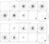 |
Fig. 1 Channel maps of the 12CO J = 1−0 and
J = 2−1 line emission towards WX Psc. The maps are corrected
for primary beam attenuation. The LSR velocities (units of km s-1) are
shown in the top-left corner of each panel. (Top) CO
J = 1−0: contours start at 4σ and are in steps
of 5σ with σ = 22 mJy beam-1. Negative
contours are plotted with the same spacing in dashed lines. The last panel shows the
continuum emission with a contour spacing of 2σ and
σ = 1.6 mJy beam-1. The synthesized beam is
|


Integrated spectra are shown in Figs. 27 and 28. They present the spatially integrated intensities obtained from the merged maps (solid black lines), the intensities observed at the source center with the 30 m telescope (dashed red lines), and the intensities spatially integrated over the observed OTF field (dashed blue lines) when they appear to be higher than the intensities observed in the merged data. This is mainly the case for the J = 2−1 line because of the smaller primary beam of the interferometer (of ~22″ in diameter at half power).
4. Results and first analysis
Velocity channel maps of the 12CO J = 1−0 and J = 2−1 line emission are shown for sixteen sources of the sample (Table 1): WX Psc, IK Tau, TX Cam, RX Boo, X Her, CRL 2362, IRAS 19475+3119, χ Cyg, CRL 2477, IRAS 20028+3910, V Cyg, IRAS 21282+5050, S Cep, OH 104.9+2.4, IRAS 23321+6545, and R Cas. In the following sections we describe the observations and analyze the results obtained for each individual source.
To analyze the size of the envelopes we systematically compared the size of the merged J = 2−1 map emission with the size derived from the single dish data alone and from the merged J = 1−0 maps (considering the different beamsizes). Conclusions are drawn in the sections devoted to individual sources, and in Sect. 5, where the results are compared with the predictions of the photodissociation models. Improved estimates of envelope sizes, based on detailed excitation analysis of the data, will be provided in forthcoming papers.
4.1. AGB stars
From previous observations it has become clear that what can be called an overall spherical symmetry is generally dominating the larger scale structures seen in AGB CSEs (e.g., arcs and halos). However, there are also observations of a few AGB stars where the stellar wind more resembles a bi-polar outflow.
Clear indications of departures from a smooth wind in terms of a relatively highly clumped medium are readily detected in observations at high angular resolution. It is not clear whether the clumps reflect inhomogeneities present already early, e.g. in the wind-accelerating zone at a distance of a few stellar radii from the star (as indicated by maser observations), or develop from instabilities (Rayleigh- Taylor, Kelvin-Helmholtz, thermal, or gravitational instabilities Myasnikov et al. 2000 in an initially relatively smooth wind.
4.1.1. WX Psc
WX Psc (IRC +10011) is an M-type (O-rich) Mira variable and an OH/IR star, with a
period of 660 days and for which a mass-loss rate of 4 × 10 yr-1
was estimated (see Table 3 for more details).
yr-1
was estimated (see Table 3 for more details).
The interferometric observations of WX Psc were carried out in June and November 2004 in the most compact array configurations. A mosaic consisting of nine fields equally spaced on a circle 13″ in radius, and spanning an area of ~70″ and 48″ in diameter (within the fields primary beam at half power) was observed at 2.6 mm and 1.3 mm, respectively. OTF observations of a square 90″-wide field were performed with the 30 m telescope to recover information on the spatial structures filtered out by the interferometer. Other details about the observations and data reduction can be found in Sect. 3 and in Table 2. The maps resulting from merging the interferometer and single dish data are shown in Fig. 1.
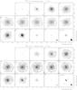 |
Fig. 2 Channel maps of the 12CO J = 1−0 and
J = 2−1 line emission towards IK Tau. The maps are corrected
for primary beam attenuation. The LSR velocities (units of km s-1) are
shown in the top-left corner of each panel. (Top) CO
J = 1−0: contours start at 4σ and are in
steps of 6σ with σ = 21 mJy beam-1.
Equivalent negative contours are plotted in dashed lines. The last panel shows the
continuum emission with a first contour and contour spacing of 3σ
and σ = 0.87 mJy beam-1. The synthesized beam is
|

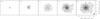 |
Fig. 3 Channel maps of the 12CO J = 2−1 line emission towards IK Tau with a spectral resolution of 2 km s-1. The LSR velocities (units of km s-1) are given in the top-left corner of each panel. Contours are plotted with a first contour and contour spacing of 4σ and σ = 45 mJy beam-1. The map center coordinates are RA 03:53:28.907, Dec 11:24:21.84 (J2000). |
Continuum emission was tentatively detected at 2.6 mm at the 3σ level, with σ = 1.6 mJy beam-1. The center of the continuum emission map lies close to the peak of the 12CO J = 2−1 emission, which suggests a positional coincidence with the geometrical center of the CSE. At 1.3 mm no continuum could be detected at the 3σ limit, with σ = 6.1 mJy beam-1.
Both the 12CO J = 1−0 and J = 2−1 emission maps show a CSE elongated along an axis oriented at PA = −45°(measured from North to East). The emission from the innermost regions looks compact in the ~4″ beam. A large difference is observed in the size of the extended halo at 2.6 mm and 1.3 mm. Data modeling will clarify if such a difference is due to the gas excitation conditions, or if the lack of emission in the outer regions is driven in part by sensitivity limitations (Schöier et al. in preparation).
The axisymmetry detected in the outermost circumstellar regions is similar to that seen in the optical by Mauron & Huggins (2006) and by Sahai et al. (2007a) at much smaller angular scales, ≲ 0.9″. VLT data obtained by Mauron & Huggins (2006) show a rather circular envelope of ~10″ in size. This also seems in agreement with our CO line maps, where the elongation is only detected at distances larger than 20″, probably due to an enhancement of apparent asymmetries in the outer shells because of the lower line opacity in these regions or a selective photodissociation of less dense gas.
4.1.2. IK Tau
IK Tau is a well-studied M-type Mira variable with a period of 500 days, and with a mass-loss rate of 1 × 10⁻⁵ M⊙ yr-1 (see Table 3 for more details).
Mosaic observations (equal to those in WX Psc, see Sect. 4.1.1) were performed in IK Tau between December 2004 and August 2005, with the array in the most compact configurations. These observations were complemented with OTF data obtained with the 30 m telescope on a square field of 110″. Other details about the observations and data reduction are given in Sect. 3 and in Table 2. The maps resulting from the merging of the interferometric and single dish observations are shown in Fig. 2.
IK Tau’s continuum emission was found to be centered at RA 03:53:28.907, Dec +11:24:21.84 (J2000), which corresponds to the brightness peak of the 12CO line emission for most of the channel maps. The continuum flux densities were found to be 9 ± 1 mJy and 28 ± 2 mJy at 2.6 mm and 1.3 mm respectively. The interferometric maps, however, suggest that the peak of the continuum emission is not spatially coincident with the centroid of the outer-shell line emission. Although the PdBI and 30 m telescope sample different spatial structures, they both detect a western elongation: while the central 12CO J = 1−0 maps (Fig. 2) bear evidence of large-scale emission stretching out along the western outer-shell regions, the J = 2−1 interferometer maps detect 2−3″ emission extending westwards of the innermost regions. Also, note a small offset of ~0″̣5 in the position of the CO J = 2−1 peak at the central channels.
There is evidence for a lack of compact emission at about 17 km s-1 (LSR) in the 12CO J = 2−1 maps. We can see this in the interferometric spectrum (Fig. 4) and it is somewhat less visible in the merged higher spectral resolution data (Fig. 3). The most likely explanation is self absorption in the line of sight, i.e. gas in the outer regions of the expanding envelope absorbs blue-shifted emission generated in the inner layers. This was also the conclusion drawn by Schöier et al. (2006a), who found a similarly narrow self-absorption feature in SMA observations of the SiO line emission towards the CSE around IRC+10216. This indirectly testifies to the presence of warm molecular gas in the inner regions, and it is even more compelling that it is not visible in the 12CO J = 1−0 line in the case of IK Tau.
Note that there is a change in the position of the J = 2−1 blue-shifted emission (Fig. 3) at ~15 km s-1, which is positionally rather coincident with a drop in emission at 19 and 21 km s-1. The warmer inner regions whose emission is absorbed by cooler gas in the outer circumstellar layers therefore appears aspherical, perhaps moving slightly faster than the outermost components (since we assume radial expansion for all components).
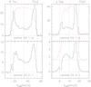 |
Fig. 4 Spectra observed towards the center of IK Tau and χ Cyg (solid lines) and obtained by spatially integrating over the emission regions (dashed lines). The latter are shown scaled for comparison. The widths at zero-power of the J = 2−1 and J = 1−0 lines appear to be similar for IK Tau. Self-absorption is well detected in the CSEs of both stars, i.e., blueshifted J = 2−1 emission from warm gas in the inner CSE regions is partly absorbed in the outer layers. In χ Cyg small wings are detected at zero-power in the J = 2−1 line. |
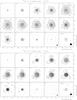 |
Fig. 5 Channel maps of the
12CO J = 1−0 and J = 2−1 line
emission towards TX Cam. The LSR velocities (units of km s-1) are shown
in the top-left corner of each panel. No primary beam attenuation correction is
applied. (Top) CO J = 1−0: contours are
plotted for 3, 7, 11, 23, and 35σ, and from there with a spacing
of 21σ and with σ = 9.6 mJy beam-1.
In the channels labeled “c” in the bottom-left corner, contours at 15 and
19σ are also plotted. Negative contours are dashed and start at
−3σ. The panel in the bottom-right corner shows the continuum
emission with contours starting at 3σ, in steps of
6σ, with σ = 0.54 mJy beam-1. The
synthesized beam is |


For IK Tau the halo sizes are also significantly different in the J = 1−0 and J = 2−1 transitions. Note that the channel maps are all corrected for primary beam attenuation. Future modeling will show if this difference is due to excitation conditions or limited by the sensitivity of the observations.
4.1.3. TX Cam
TX Cam is an M-type Mira variable with a period of 557 days and a mass-loss rate of 7 × 10⁻⁶ M⊙ yr-1 (see Table 3 for more details).
The interferometric observations of TX Cam were performed in November and December 2005 in the most compact array configurations. TX Cam was observed in track-sharing mode together with IRAS 06192+4657, which will be published in a forthcoming paper. OTF observations of a square 110″-side field were performed with the 30 m telescope. Other details about the observations and data reduction are given in Sect. 3 and in Table 2. The data resulting from merging the interferometric and single dish observations are shown in Fig. 5.
The continuum emission was found to be centered at RA 05:00:51.157, Dec +56:10:54.00 (J2000). The derived continuum fluxes are 10.1 ± 0.6 and 24.5 ± 0.9 mJy at the frequencies of the J = 1−0 and J = 2−1 transitions, respectively. The continuum position is coincident with the 12CO emission peak at the highest expansion velocities where the emission is more compact. For the central velocity channels the emission seems to be distributed in a hook-like structure, well detected at 14 km s-1.
Although the structure of the CSE around TX Cam appears to be round, signs of asphericity are observed at different scales. The innermost regions show the presence of a conspicuous hook-like structure, well resolved in the J = 2−1 line. The elongation of the J = 2−1 emission in the outermost layers towards the southeast and to the northwest seems consistent with the hook-like (helicoidal) structure observed in the innermost and also outer regions, in both the 2.6 mm and 1.3 mm maps. This elongation, however, can only be understood as part of a larger halo. The halo seen in the central channels of the 12CO J = 1−0 and J = 2−1 maps shows an extension towards the north/northwest (where an arc seems to have formed) and the southeast.
Figure 6 shows an overlay of the 12CO J = 1−0 and J = 2−1 emission, which provides a good view of the circumstellar gas distribution around TX Cam. The brightest 12CO J = 2−1 emission mapped with the interferometer (which provides the highest resolution) is plotted together with the lowest-brightness contours from the 12CO J = 1−0 data shown in Fig. 5 (which best traces the halo extent). When convolving the 12CO J = 2−1 data with the synthesized beam obtained for the J = 1−0 transition both morphologies look very similar, except for the outer halo regions. All maps are affected by the primary beam attenuation, since the molecular emission in TX Cam is extended beyond the field of view of the PdBI antennas. The J = 2−1 single-dish maps suggest a halo around TX Cam as large as the one observed in the merged J = 1−0 data (Fig. 5) but no trace of it is left in the merged maps. When comparing the single-dish and merged data (see Fig. 27) we see that a significant part of the halo emission is not present in the merged maps due to the limited field of view of the PdBI antennas. This has consequences for the mapping quality and reduces the confidence level by which the outer structures can be reliably mapped to the 7σ threshold level. Note that Fig. 27 shows the 4 km s-1 and 1 km s-1 resolution integrated spectra from the TX Cam’s merged data. The 4 km s-1 resolution spectrum, obtained with the 1 MHz filterbank, provides the better S/N ratio. The 1 km s-1 resolution spectrum provides enough resolution to identify velocity channels affected by interstellar gas along the line of sight.
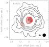 |
Fig. 6 Composite image of TX Cam overlaying the 12CO J = 1−0 emission in the outermost regions (black contours) and the 12CO J = 2−1 emission from the interferometric data alone (red contours). Interferometric data alone provide a more genuine rendition of the innermost structure. The synthesized beams of both datasets are plotted in the bottom-right corner. |
Spiral structures have been identified in the CSEs around some few AGB stars. A large spiral pattern was clearly seen in the optical in CRL 3068 (Mauron & Huggins 2006). Recent interferometric observations of the HC3N J = 5−4 line emission from CIT 6 suggest the presence of a helicoidal distribution (Dinh-V.-Trung & Lim 2009). Helicoidal gas distributions are so far interpreted to be a consequence of the presence of a binary (see e.g. Mauron & Huggins 2006).
4.1.4. RX Boo
RX Boo is an M-type semiregular variable (SRb) with a period of 340 days and a mass-loss rate of 5 × 10⁻⁷ M⊙ yr-1 (see Table 3 for more details).
The interferometric observations of RX Boo were performed in June and November 2004 with the most compact array configurations. RX Boo was observed in track-sharing mode together with S CrB, whose data will be presented in a forthcoming paper. We performed OTF observations of a square 90″-size field with the 30 m telescope. Other details about the observations and data calibration are given in Sect. 3 and in Table 2. Following the CLEANing procedure described in Sect. 3.3, we show in Fig. 7 the SDI-cleaned maps resulting from merging interferometric and single-dish observations. Compared to HOGBOM, the SDI algorithm is less prone to produce spurious halo fragmentation (which was specially significant in the J = 2−1 maps).
The derived continuum fluxes of RX Boo are 7 ± 1 and 20 ± 3 mJy at 2.6 and 1.3 mm, respectively. The emission at 1.3 mm was found to be centered at RA 14:24:11.626, Dec +25:42:13.18 (J2000). This is close to the CO J = 2−1 emission peaks but does not match the position of the peaks observed in the CO J = 1−0 maps. Although the maps obtained for both CO lines show similar structures, the J = 2−1 emission from the innermost CSE regions is likely to be affected by a higher line opacity. The J = 1−0 data hence seem to better reveal the actual CSE mass distribution.
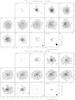 |
Fig. 7 Channel maps of the 12CO J = 1−0 and
J = 2−1 line emission towards RX Boo. The LSR velocities
(units of km s-1) are shown in the top-left corner of each panel. No
primary beam attenuation correction is applied. (Top) CO
J = 1−0: contours are plotted from 3σ in
steps of 3σ with σ = 16 mJy beam-1.
Equivalent negative contours are plotted with dashed lines. The last panel shows
the continuum emission with contours starting at 3σ in steps of
3σ with σ = 0.6 mJy beam-1, and the
synthesized beam in the bottom-right corner of size |


The CO line emission found in RX Boo shows axial symmetry, with a symmetry axis at PA ~ 50°. In the central CO J = 1−0 channel maps, between 0 and 2 km s-1, we can see a structure elongated perpendicularly to the symmetry axis. This elongation is more obvious in the J = 2−1 channel maps with velocities between −4 and 8 km s-1. From + 4 to 8 km s-1, the CO J = 1−0 peak emission is displaced toward the northeast along the symmetry axis, forming an arc-like structure at ~5−7′′ from the center. At 10 km s-1 the emission peak is slightly displaced to the southwest along the symmetry axis. A counterpart of this structure is also seen at blue-shifted velocities: a southwest displacement from −6 to −2 km s-1, followed by a northeast offset at −8 km s-1. In Fig. 8 we present a position-velocity (P-V) diagram along the symmetry axis is presented. Arrows indicate the position of the highest-velocity emission. This distribution in position and velocity resembles that seen in the central part of several post-AGB CSEs (see e.g. Castro-Carrizo et al. 2002; and Bujarrabal et al. 2007), and also in X Her (Sect. 4.1.5). In those cases, we identify an hour-glass structure in expansion, sometimes rather a ring or disk-like structure, more or less embedded within a more extended rounded CSE. The components identified at the highest-velocities in most pPNe (e.g. Castro-Carrizo et al. 2002), which come from fast moving extended lobes, are not detected for RX Boo though. A specific modeling is needed to draw firmer conclusions about the mass distribution in the CSE around RX Boo, and particularly to conclude about the presence of expanding lobes, or merely an equatorial mass loss enhancement.
Finally, the extension of the halo imaged in J = 2−1 line emission (see Fig. 7 and also Table 4) is constrained by the primary beam attenuation. This may also be the case for the J = 1−0 maps, but to a lesser degree. In Fig. 27 we can see that the profile obtained by integrating the single-dish emission (in blue) is much higher than the one obtained from merged maps (in black).
4.1.5. X Her
X Her is an M-type semiregular variable (SRb) with a period of 95 days. Previous CO data show a composite line profile, with a narrow spectral feature centered on a broader component (Kahane & Jura 1996; Kerschbaum & Olofsson 1999; Knapp et al. 1998; Olofsson et al. 2002). High-resolution data indicate that the broad emission plateau arises from a bipolar outflow, while the narrow emission feature comes from a disk, which was interpreted to be in rotation (Nakashima 2005). Mass-loss rates of 1.5 and 0.4 × 10⁻⁷ M⊙ yr-1 were deduced for the broad and narrow components (see Table 3 for more details).
The interferometric observations of X Her were performed in February and March 2005 in intermediate configurations of the PdBI, and were carried out in track-sharing mode together with IRAS 23321+6545 (Sect. 4.2.4). OTF line observations of a square 110″-wide field were performed with the 30 m telescope. Other details about the observations and data reduction are given in Sect. 3 and in Table 2.
The maps resulting from merging interferometric and single dish observations are shown in Fig. 9. The single-dish J = 2−1 data lacked sensitivity to achieve proper merging with the PdBI visibilities. Imaging was difficult enough that we caution against over-interpreting extended emission features (at the 6 × σ level) visible in the three central channels of the 12CO J = 2−1 maps (Fig. 9, marked c in the bottom-left corner). The distribution found for the other channels is however consistent with that obtained for 12CO J = 1−0, confirming the circumstellar structure obtained in the 12CO J = 2−1 line.
We detected continuum emission in the interferometric data at 2.6 and 1.3 mm. By fitting in the uv-plane the more sensitive 1mm visibilities, we found that the continuum emission is centered at coordinates RA 16:02:39.14, Dec 47:14:25.55 (J2000). The continuum flux densities are 2.8 ± 0.4 mJy and 13.5 ± 0.6 mJy at 2.6 and 1.3 mm respectively.
The structure obtained in 12CO J = 1−0, confirmed by the 12CO J = 2−1 data, is axisymmetric, even more clearly than for RX Boo (Sect. 4.1.4). A position-velocity (P-V) gradient was already detected by Kahane & Jura (1996) and Nakashima (2005). Our maps show for the first time an hourglass structure similar to that seen for M 2-56 (Castro-Carrizo et al. 2002), except for the lobes’ tips that are not seen in X Her. At the systemic velocity of −73 km s-1, we see a disk-like distribution perpendicular to the symmetry axis. At the expansion velocities from −81 to −79 km s-1 and from −65 to −67 km s-1 we see parts of the expanding hourglass with higher projected velocities. Arc-like distributions are seen opening outwards in these channels, corresponding to the inner parts of the lobes. No other faster components are detected. At lower expansion velocities, from −77 to −75 km s-1 for the westernmost lobe, and from −69 to −71 km s-1 for the easternmost one, the hourglass structure is clearly seen, depending on the projected velocity of the different parts of the walls of the hourglass. Similar structures are observed and modeled in the early post-AGB CSEs of 89 Her (Bujarrabal et al. 2007) and, as mentioned before, M 2-56 (Castro-Carrizo et al. 2002). These two objects have very different symmetry-axis inclinations with respect to the sky plane. By comparison, the CO distribution in X Her suggests a relatively low inclination angle, but proper modeling is needed to corroborate this conclusion.
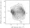 |
Fig. 8 Position-velocity diagram along the symmetry axis, at PA = 50°, of the 12CO J = 1−0 emission maps towards RX Boo. Contours are equivalent to those shown in Fig. 7. |
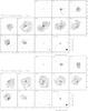 |
Fig. 9 Channel maps of the 12CO J = 1−0 and
J = 2−1 line emission towards X Her, at the LSR velocities
(units of km s-1) specified in the top-left corner of each panel. No
primary beam attenuation correction is applied. (Top) CO
J = 1−0: contours are plotted from and with a spacing of
2.5σ, where σ = 10 mJy beam-1.
Equivalent negative contours are plotted in dashed lines. The last panel presents
the continuum emission from and with a spacing of 2.5σ, with
σ = 0.35 mJy beam-1. The synthesized beam is
|


In Fig. 27 we show the spectra obtained from our observations. The merged data are presented with solid lines, and the profiles obtained at the source center with the 30 m single-dish are shown with dotted lines. To avoid introducing artifacts in the profiles due to the CLEANing procedure, the merged-data profiles were obtained directly from the uv-data.
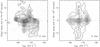 |
Fig. 10 (Left): position-velocity diagram along the symmetry axis at PA = 45° of the 12CO J = 1−0 emission towards X Her. (Right): the same along an axis at PA = −45°. Contours are equivalent to those shown in Fig. 9. |
The P-V diagram along the symmetry axis, at PA = 45°(see Fig. 10), resembles that obtained for M 2-56, or to the central part of that of M 1-92 (Alcolea et al. 2007). The diagram obtained along the perpendicular axis, at PA = −45°, shows that we do not detect any decrease in brightness in the center with the spatial resolution we have in this direction (~1.6″). If we assume an expansion velocity of 5−10 km s-1 for the remnant of the AGB CSE, this would indicate that mass loss was active until at least 100 yr ago (where we took as spatial limit the spatial resolution, at a distance of 140 pc). With the current data, and without a detailed modeling, we cannot relate the presence of the axial molecular gas distribution to the end of the mass-loss phase in X Her.
The kinematics deduced from our maps are dominated by the axial gas distribution. Deducing an expansion velocity for a possible remnant of a previous spherical AGB wind is not straightforward. If we assume that the narrow central component of the CO profiles comes from the remnant of a spherical AGB outflow, we deduce an expansion velocity for the spherical AGB wind of ~5 km s-1, which is a relatively low value (see e.g. Bujarrabal et al. 2001).
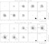 |
Fig. 11 Channel maps of the 12CO J = 1−0 and
J = 2−1 emission toward CRL 2362 at the LSR velocities (units
of km s-1) specified in the top-left corner of each panel. No primary
beam attenuation correction is applied. (Top) CO
J = 1−0: contours are plotted from and with a spacing of
3σ, where σ = 7 mJy beam-1.
Negative contours are plotted in dashed lines with the same spacing. The last
panel presents the continuum emission with a first contour and contour spacing of
3σ, with σ = 0.3 mJy beam-1. The
synthesized beam is |


Finally, no rotating disk is detected in our data, contrary to what was suggested by Nakashima (2005), who deduced the presence of a Keplerian disk of ~6″ in diameter from a brightness distribution compatible with our data. The CO data presented here confirm that the structure seen by Nakashima (2005) belongs to an expanding bipolar distribution, as was also alternatively mentioned in their paper. If a Keplerian disk would exist, we estimate that it should be smaller than 2″.
4.1.6. CRL 2362
CRL 2362 is an OH/IR star with a mass-loss rate of 1.9 × 10⁻⁵ M⊙ yr-1 (see Table 3 for more details). It was detected in OH at 1612 MHz by Silverglate et al. (1979).
CRL 2362 was observed in the track-sharing mode together with V CrB in intermediate array configurations, in December 2004 and March 2005. A 3 × 3 points map was observed with the 30 m telescope to cover a field of ~35″ in size at 1.3 mm. Four additional points were observed outside this region to ensure that no emission is detected outside the observed field. Other details about the observations and data calibration are given in Sect. 3 and in Table 2. The imaging of the merged data was difficult for CRL 2362, specially for the J = 2−1 data. The contrast of weights between both data sets made it impossible to recover all the flux filtered out by the interferometer in the merged data, which is actually relevant for the J = 2−1 channel maps (see Fig. 27). The resulting maps from the merged data are shown in Fig. 11.
In Fig. 27 we show the profile (solid black line) obtained from the single-dish observations at zero spacing, after merging with the PdBI data. This corresponds to the integrated flux within the PdBI primary beam. In solid red line we show the flux integrated in the merged data maps, which allows us to quantify the amount of flux present in the final maps (Fig. 11). The large loss of flux in the maps shows the difficulties to merge interferometric and single-dish data in the case of CRL 2362. Finally, the profile obtained with the 30 m telescope at the source center (red dotted line) shows that a significant part of the emission is more extended than the 30 m telescope beam at 2.6 mm.
The emission shown in Fig. 11 is relatively compact, which is likely due to some extended emission, which remains undetected in the J = 2−1 channel maps. In addition, no continuum is detected within a 1 sigma noise level of 0.3 and 0.6 mJy beam-1 at 2.6 and 1.3 mm, respectively.
4.1.7. χ Cyg
χ Cyg is an S-star Mira variable with a period of 407 days and a mass-loss rate of 5.0 × 10⁻⁷ M⊙ yr-1 (see Table 3 for more details).
The PdBI observations of χ Cyg were performed between September 2005 and May 2006 with the most compact array configurations, and in track-sharing mode together with IRAS 20028+3910 (see Sect. 4.2.2). OTF observations of a square 90″-size field were performed with the 30 m telescope. Additional observational and calibration details are given in Sect. 3 and in Table 2. The CO maps resulting from merging interferometric and single dish observations are shown in Fig. 12.
The angular size of the outermost regions detected in the 12CO J = 1−0 and J = 2−1 maps seems to be similar to the size of the PdBI primary beam at half power, which is certainly because the maps are not corrected for the primary beam attenuation. Modeling the data, and particularly the 30 m-telescope 100″-field data, will allow us a better estimate of the size of this CSE.
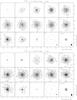 |
Fig. 12 Channel maps of the 12CO J = 1−0 and
J = 2−1 line emission toward χ Cyg at the
LSR velocities (units of km s-1) specified in the top-left corner of
each panel. No primary beam attenuation correction is applied.
(Top) CO J = 1−0: contours are plotted from
4σ, with a spacing of 8σ, where
σ = 10 mJy beam-1. In the panels marked with
c in the bottom-left corner the first four contours are at 4,
12, 20 and 28σ, and from there the spacing is
20σ. Equivalent negative contours are plotted in dashed lines.
The last channel presents the continuum emission with a first contour and contour
spacing of 3 and 6σ respectively, where
σ = 0.4 mJy beam-1. The synthesized beam, plotted in
the bottom-right corner of last panels, is |

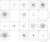 |
Fig. 13 Some channel maps obtained for the CO J = 1−0 (upper) and J = 2−1 (lower) emission toward χ Cyg with 1 km s-1 spectral resolution (LSR velocities specified in the top-left corner of each channel, in km s-1). In the J = 1−0 channel maps, contours are plotted from 3σ, with a spacing of 6σ, with σ = 14 mJy beam-1. In the J = 2−1 channel maps, contours are plotted from 4σ, with a spacing of 6σ, with σ = 30 mJy beam-1. |
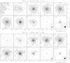 |
Fig. 14 Channel maps of the 12CO J = 1−0 and
J = 2−1 line emission toward V Cyg at the LSR velocities
(units of km s-1) specified in the top-left corner of each panel. No
primary beam attenuation correction is applied. (Top) CO
J = 1−0: contours are plotted at 5, 12, 24, and
42σ and from there with a spacing of 20σ,
where σ = 7.8 mJy beam-1. Equivalent negative
contours are plotted in dashed lines. The last panel presents the continuum
emission with a first contour and contour spacing of 3σ, where
σ = 0.4 mJy beam-1. The synthesized beam, plotted in
the bottom-right corner of last panels, is |


We slightly resolved the 1.3 mm continuum emission (Fig. 12). The continuum centroid seems to coincide with the line emission centroid
at the map center, with coordinates RA 19:50:33.907, Dec 32:54:50.40
(J2000). The peak of the continuum emission is slightly shifted however
(at a [0.2″,0.2″] offset) toward the position at which we detect the CO emission at the
highest expansion velocities. The continuum in χ Cyg is particularly
bright compared to the other stars shown in this paper, with a total of 15.8 ± 0.7 mJy
and 65 ± 3 mJy, at 2.6 and 1.3 mm respectively. These results are obtained by fitting
the data in the uv-plane with an elliptical Gaussian with a size of
 (± 0.07″) at PA = 56° (± 13°).
The line emission in the central channels peaks at the map center. At the highest expansion velocities, the 12CO emission is however slightly displaced with respect to the map center. This can be better seen in Fig. 13, where the highest expansion-velocity channels are presented with 1 km s-1 resolution. At velocities between −3 and 0 km s-1 the emission is coming from an elongated region displaced ~3″ eastwards from the brightness peak observed between 2.5 and 3.5 km s-1. At 3.5 km s-1, at an offset of ~[3″,3″] we see a significant relative minimum in both CO lines. We could speculate that this is due to the presence of a higher excitation region within the CO envelope where CO may be dissociated. Note that the high velocity emission seen at ~0 km s-1 is detected close to this position, but not coincident with it.
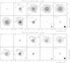 |
Fig. 15 Channel maps of the 12CO J = 1−0 and J = 2−1 line emission toward S Cep at the LSR velocities (units of km s-1) specified in the top-left corner of each panel. No primary beam attenuation correction is applied. (Top) CO J = 1−0: contours are plotted at 3, 6, 9, and 12σ, and from there with a spacing of 10σ, where σ = 7.9 mJy beam-1. Equivalent negative contours are plotted in dashed lines. The last panel presents the continuum emission with a first contour and contour spacing of 3σ, where σ = 0.6 mJy beam-1. The synthesized beam, plotted in the bottom-right corner of last panels, is 3″̣3 × 2″̣8 in size, with PA = 21°. (Bottom) CO J = 2−1: contours are plotted from and with a spacing of 6σ, where σ = 18 mJy beam-1. In the panels marked with c in the bottom-left corner, from the contour at 24σ the spacing is 12σ. Equivalent negative contours are plotted in dashed lines. The last panel presents the continuum emission with a first contour and contour spacing of 3σ, where σ = 1.4 mJy beam-1. The synthesized beam, plotted in the bottom-right corner of last panels, is 1″̣7 × 1″̣3 in size, with PA = 27°. The primary beams are plotted at half power in dotted lines in the last panels of the channel maps. The central coordinates are RA 21:35:12.830, Dec 78:37:28.19 (J2000). |
We also notice that compact 12CO J = 2−1 emission is not detected between 0.5 and 2.5 km s-1. In particular, we see at −0.5 km s-1 that the compact J = 2−1 emission is much brighter than at 0.5 km s-1. Also the line profile obtained from the interferometric data (which is sensitive to compact emission) presents a minimum at these velocities (see Fig. 4). Note that no ISM contribution is detected in the single dish 2.6 mm observations. The emission minimum at ~0.5 km s-1 probably results from CSE self absorption, i.e. from absorption by CO molecules in the outer layers with relatively low excitation (see Sect. 4.1.2). Also, a counterpart of the elongation seen at ~−1 km s-1 in the CO J = 2−1 emission may exist at redshifted velocities, between 18 and 21 km s-1, mainly in the CO J = 1−0 emission (see Fig. 13). We do not see a unique symmetry axis for all the mentioned features. The CO emission detected at higher expansion velocities in both lines seems to be elongated along axes of PA from 30° (at 19.5 km s-1) to 85°(at −0.5 km s-1). This is compatible with the small elongation found in the 1.3 mm continuum and with the brightness minima detected at ~3.5 km s-1. Based on this, we speculate that there may be aspherical winds developing within the large CSE of χ Cyg.
The mapping of χ Cyg’s extended envelope is limited by PdBI’s primary beam attenuation, more severely at 1.3 mm, as we can deduce by comparing the blue and black profiles in Fig. 27. A better estimate of the envelope size can be made by analyzing the OTF maps (see Table 4). We deduce that χ Cyg extends ≳ 100″, at least for the coolest gas component detected in the CO J = 1−0 maps.
4.1.8. V Cyg
V Cyg is a carbon-rich Mira variable with a period of 421 days. The mass-loss rate estimated to be 9.0 × 10⁻⁷ M⊙ yr-1 (see Table 3 for more details).
The PdBI observations of V Cyg were performed in June and November 2004 with the most compact array configurations, in track-sharing mode together with IRAS 21282+5050 (Sect. 4.2.3). OTF observations in a square 90″-size field were obtained with the 30 m telescope. Other observational and calibration details are given in Sect. 3 and in Table 2. The maps resulting from merging interferometric and single-dish observations are shown in Fig. 14.
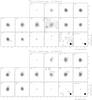 |
Fig. 16 Channel maps of
the 12CO J = 1−0 and J = 2−1 line
emission toward OH 104.9+2.4 at the LSR velocities (units of km s-1)
specified in the top-left corner of each panel. No primary beam attenuation
correction is applied. (Top) CO J = 1−0:
contours are plotted from, and with a spacing of, 0.032 Jy beam-1.
Equivalent negative contours are plotted in dashed lines. The last panel presents
the continuum emission with a first contour and contour spacing of
3σ, where σ = 0.65 mJy beam-1. The
synthesized beam, plotted in the bottom-right corner of last panels, is
|


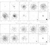 |
Fig. 17 Channel maps of the
12CO J = 1−0 and J = 2−1 line
emission toward R Cas at the LSR velocities (units of km s-1) specified
in the top-left corner of each panel. No primary beam attenuation correction is
applied. (Top) CO J = 1−0: contours are
plotted from 3σ and from there with a spacing of
3σ, where σ = 11mJy beam-1.
Equivalent negative contours are plotted in dashed lines. The last panel presents
the continuum emission with a first contour and contour spacing of
4σ, where σ = 0.6 mJy beam-1. The
synthesized beam, plotted in the bottom-right corner of last panels, is
|


 |
Fig. 18 (Left:) channel maps of the 12CO J = 2−1 line emission toward R Cas equivalent to those shown in Fig. 17, resulting from CLEANing with the SDI method. Contours are plotted at 3.5, 7, 10.5, 14, 19 and 24σ and from there each 8σ, where σ = 29 mJy beam-1. Although the results obtained with different CLEANing methods allow emphasizing different structures, the resulted brightness distributions are very compatible. (Right:) the azimuthal average of the brightness distribution around the center is shown, at the systemic velocity (25 km s-1), for both 12CO J = 1−0 and J = 2−1 emission. Peaks are found at the same radius for both transitions. |
The CO J = 2−1 extended emission presents an axisymmetrical triangular shape along an axis of PA ~ −45°. In the J = 1−0 line this elongated shape is less pronounced, but appears in the outermost regions. In contrast, the CSE innermost regions seem to be rather spherical. In addition, we find interstellar contamination at velocities between ~−5 and 1.5 km s-1, which is more important in the J = 1−0 line (see Fig. 27), and also visible in the maps in the northeast of V Cyg.
Line emission is detected up to the primary beam size at half power, which is likely due to that the maps are not corrected by primary beam attenuation. The 30 m-telescope data show that V Cyg’s CO emission extends further out than that mapped in Fig. 14. We can see in Fig. 27 that more flux is detected in the single-dish observations, specially in the CO J = 2−1 maps.
The continuum emission is shown in the last panels of Fig. 14. The fluxes 7.2 ± 0.5 and 17.0 ± 0.9 mJy are derived for the continuum at 2.6 and 1.3 mm respectively.
4.1.9. S Cep
S Cep is a carbon-rich Mira variable with a period of 487 days and with a mass-loss rate of 1.2 × 10⁻⁶ M⊙ yr-1 (see Table 3 for more details).
The PdBI observations of S Cep were performed between July and November 2004 with the most compact array configurations, in track-sharing mode together with T Cep. OTF observations in a square 90″-size field were obtained with the 30 m telescope. Other details on the observations and data calibration are given in Sect. 3 and in Table 2. The maps resulting from merging interferometric and single dish observations are shown in Fig. 15.
The CO J = 1−0 line emission presents a largely circular symmetry in the outermost regions. In the CO J = 2−1 line, the outer halo is not well mapped, due to the limited sensitivity of the merged data. The brightest CO J = 2−1 emission is rather well centered in the channel maps at high expansion velocities, i.e. at the LSR velocities −39 and 9 km s-1. At all the other velocities the J = 2−1 line emission seems to be elongated, the centroid of the most compact emission being slightly displaced to the southeast. Similar features are observed in the innermost regions of the CO J = 1−0 line emission.
In the spectra shown in Fig. 27 we can see apparent absorptions from ~−6 to +1 km s-1. Their larger presence in the CO J = 1−0 maps than in the J = 2−1 ones suggests that this is due to ISM contamination.
Continuum is detected at 2.6 and 1.3 mm, the derived fluxes are 4.6 ± 0.7 and 11.3 ± 1.4 mJy respectively.
4.1.10. OH 104.9+2.4
OH 104.9+2.4 is an OH/IR star with a period of 1460 days. The mass-loss rate estimated by Heske et al. (1990) is lower by more than one order of magnitude than the values derived from e.g. OH 1612 MHz emission or IR continuum in OH/IR stars. This will be investigated in more detail in the analysis of the data presented in this paper in a forthcoming paper (see Table 3 for more details about OH 104.9+2.4).
The interferometric observations of OH 104.9+2.4 were performed between August and December 2004 with the most compact array configurations, in track-sharing mode together with R Cas (see Sect. 4.1.11). Since a small angular size was estimated for the CSE around OH 104.9+2.4, we only performed observations at the source center with the 30 m telescope (shown in dashed red lines in Fig. 27) to recover the zero-spacing flux. Other details about the observations and data reduction are given in Sect. 3 and in Table 2.
The maps shown in Fig. 16 result from adding the uv-plane zero spacing to the interferometric data. The imaging of the merged data presents almost no difference with respect to the purely interferometric results, except for the channels contaminated by ISM emission (at ~−23 and −2 km s-1). In Fig. 27 we see a global difference of about 30% between single-dish profiles (dashed) and the interferometric data. We cannot easily distinguish between having some flux filtered out by the interferometer and a possible calibration inconsistency between the data sets.
CO emission observed towards OH 104.9+2.4 is relatively compact, extending less than 4″. As mentioned before, we can see ISM contamination at ~−23 and −2 km s-1 in Fig. 16. As expected, its contribution is more important in the CO J = 1−0 line than in the J = 2−1 line.
Continuum emission is not detected, as shown in the last panels of the channel maps in Fig. 16, with σ = 0.65 and 1.4 mJy at 2.6 and 1.3 mm respectively.
4.1.11. R Cas
R Cas is an M-type Mira variable with a period of 431 days and with a mass-loss rate of 9 × 10⁻⁷ M⊙ yr-1 (see Table 3 for more details).
The PdBI observations of R Cas were performed in track-sharing mode, with OH 104.9+2.4 (Sect. 4.1.10). OTF observations in a square 90″-size field were obtained with the 30 m telescope. See Sect. 3, Sect. 4.1.10 and Table 2 for more details about the observations and data reduction. The resulting maps are shown in Fig. 17. The synthesized beam of the J = 2−1 channel maps is increased (by 40%) with some tapering to reduce the clumpiness, which explains the difference to the 1.3 mm continuum-map beam.
Arcs are well detected at the five central channels of the J = 1−0 maps displayed in Fig. 17. Although these arcs may be part of larger ring-like distributions, we have no clear evidence of complete structures. We note that the arcs seen in the outermost regions, for instance at the systemic velocity, are not equally spaced from the center. Also, the rounded structure seen in the innermost regions of R Cas resembles the hook-like distribution seen in TX Cam (see the J = 2−1 maps in Fig. 5).
The presence of arcs, the weak brightness of the extended emission, and the primary beam attenuation make it difficult to map the outermost circumstellar envelope at 1.3 mm. The CO J = 2−1 maps obtained by tapering the original uv-data (shown in Fig. 17) show a brightness distribution compatible with that seen in the J = 1−0 maps. Note that by CLEANing the same data with different methods, including SDI, all the main clumpy features remain (see Fig. 18). Finally, we note that the mapping of the most extended CO emission is biased by the PdBI primary beam attenuation, mainly at 1.3 mm, as we can see in Fig. 27.
In the maps the CO J = 1−0 and J = 2−1 line emission is found to be displaced and elongated toward the southeast and the north (rather northwest in the J = 2−1 maps), respectively at high expansion velocities (in the channels at 13 and 37 km s-1). We do not have enough sensitivity however to interpret these features.
The last plot of Fig. 18 presents the azimuthally averaged (normalized) brightness from the 2.6 and 1.3 mm maps, at the systemic velocity (25 km s-1), as a function of the distance from the central star. In both maps we obtain relative maxima at 6″̣2 and 12″̣8 from the center. If we adopt a distance of 172 pc and an expansion velocity of 15 km s-1, these azimuthal-averaged peaks would correspond to time scales of 350 years, possibly indicating modulations of the mass-loss rate on these time scales. We cannot conclude from our maps however if these variations present a perfect spherical symmetry.
Continuum emission is detected, as shown in the last panels of the channel maps in Fig. 17. By fitting the continuum visibilities in the uv-plane, we obtain the fluxes of 13 ± 0.7 and 45 ± 2 mJy at 2.6 and 1.3 mm, respectively. The 1.3 mm continuum emission is only marginally resolved (0.3 ± 0.1″).
4.2. Post-AGB objects
Most of the early post-AGB stars present strongly aspherical (often axisymmetrical) CSEs, resulting from the interaction of axial fast winds with the CSE formed in the AGB phase. The COSAS project also aims to find clues to understand the burst of the axial post-AGB winds, which are thought to arise when the AGB phase ends. We hence included in our sample seven well-identified early post-AGB sources, four of which are presented in this section. Particularly, two of them, IRAS 21282+5050 and IRAS 23321+6545, did not digress so far from spherical symmetry.
4.2.1. IRAS 19475+3119
IRAS 19475+3119 is a post-AGB nebula surrounding a yellow F3Ib star. The absence of OH and H2O maser emission suggests that it is C-rich. We will adopt for this source a distance D = 4.9 kpc which is similar to that adopted by other authors (Sánchez Contreras et al. 2006; Sahai et al. 2007b; Hrivnak & Bieging 2005; Bujarrabal et al. 2001). IRAS 19475+3119 presents a strongly axisymmetric nebula in molecular line emission (Sánchez Contreras et al. 2006); its prominent axis, at PA ≈ 80°, is associated with a fast bipolar outflow with an inclination angle i ≈ 30° with respect to the plane of the sky. HST images (Sahai et al. 2007b) show also a secondary lobe at PA ≈ −45°. Sarkar & Sahai (2006) deduced similar values for the extent and CSE total mass based on the analysis of FIR and submm continuum data.
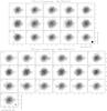 |
Fig. 19 Channel maps of the 12CO J = 1−0 and
J = 2−1 emissions (in contours) toward IRAS 19475+3119 at the
LSR velocities (units of km s-1) specified in the top-left corner of
each panel. In the background, in grey scale, the optical image obtained by (Sahai et al. 2007b) is shown for comparison. No
primary beam attenuation correction is applied. (Top)
CO J = 1−0: contours are plotted from and with a spacing of
2.8σ, where σ = 6.9 mJy beam-1.
Equivalent negative contours are plotted with dashed lines. Contours presenting
relative minima in the CSE are plotted in grey (red in the electronic version).
The synthesized beam is |

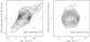 |
Fig. 20 Left: position-velocity diagram along the symmetry axis at PA = 90° of the 12CO J = 2−1 emission maps towards IRAS 19475+3119. Contours are plotted from 2σ with the same spacing. Right: the same along an axis at PA = 0°. Contours are plotted from 6σ, with a spacing of 3σ (σ = 11 mJy beam-1). |
The PdBI observations of IRAS 19475+3119 were obtained in January and February 2005 in the most extended array configurations. IRAS 19475+3119 was observed by sharing tracks with CRL 2477, whose data are shown in Sect. 4.2.5. The 30 m telescope observations obtained toward the center of IRAS 19475+3119 show line profiles similar to those obtained from the interferometric data (Fig. 28). The small difference between the J = 2−1 profiles is likely due to an inconsistency in the calibration of the data sets. No significant flux is filtered out by the interferometer. Other details about the observations and data calibration are given in Sect. 3 and in Table 2.
No continuum emission is detected with rms limits of 0.4 and 0.6 mJy at 2.6 and 1.3 mm, respectively.
The PdBI maps of the 12CO J = 1−0 and J = 2−1 emission in IRAS 19475+3119 are shown in Fig. 19. The center of the plots (RA 19:49:29.561, Dec 31:27:16.29) corresponds to the brightest point in the optical. Although in the central channels, at 17 and 21 km s-1, the shape of the CSE emission is more or less round, the observed CO distribution is strongly axisymmetric according to the presence of two main high-velocity lobes. The CO emission is distributed at different positions along the symmetry axis for different velocities. In the optical (Sahai et al. 2007b), IRAS 19475+3119 presents a quadrupolar structure resulting from collimated winds along two main axes (see background image in the channel maps). The main axis of the CO distribution is certainly related to the axial symmetry of the most prominent bipolar lobes, seen in the optical with PA = 90°. We find CO emission at the highest expansion-velocity along these optical structures, as well as emission minima along the axis at the central velocities, from 1 to 37 km s-1. Curved brightness distributions typical of CO emission from a projected hourglass-like structure are seen at 9 km s-1 and at 25 km s-1 (see e.g. Bujarrabal et al. 1998; Castro-Carrizo et al. 2002). The position-velocity (P-V) diagrams along the symmetry axis (PA = 90°) and the perpendicular one (PA 0°), see Fig. 20, are very similar to those found in other pPNe presenting axisymmetric distributions (see Bujarrabal et al. 1998; Castro-Carrizo et al. 2002). In addition, IRAS 19475+3119 presents in the optical (Sahai et al. 2007b) another pair of lobes, aligned at PA = −55°. In Fig. 19 we find a counterpart in CO of the presence of these lobes with PA = −55° in the 12CO J = 2−1 maps at velocities from 13 to 25 km s-1. CO-rich gas seems to be symmetrically distributed along this axis, and some point-like symmetry is also identified. Although most of the CO emission is within the quadrupolar structure seen in the optical, we also detect emission outside the optical lobes (for instance at the offset position [1″,2″], at velocities from 5 to 29 km s-1).
In the P-V diagram along the symmetry axis (PA ≈ 90°) we see that both brightness peaks are at positive offsets with respect to the center, where the optical peak is. In the P-V diagram along the perpendicular axis (PA ≈ 0°) the ring-like structure presents some asymmetry between north and south. Both asymmetries may be related with respect to the assumed optical center to the presence of the secondary lobes (with PA = −55°). We cannot discard the possibility of an erroneous assumption in the position of the nebula center by 0″̣3. In addition, the optical image at the center may be affected by opacity, which could explain that the optical emission peaks slightly westward with respect to the position of the central star.
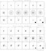 |
Fig. 21 Channel maps of the 12CO J = 1−0 and
J = 2−1 line emission (in contours) toward IRAS 20028+3910 at
the LSR velocities (units of km s-1) specified in the top-left corner
of each panel. No primary beam attenuation correction is applied.
(Top) CO J = 1−0: contours are superposed on
HST images by Ueta et al. (2000), and
plotted from 2.6σ, with a spacing of 3σ, where
σ = 7.1 mJy beam-1. In the panels marked with
c in the bottom-left corner the first contours are at 6, 10,
15, 21, 27, 34σ and from there every 15σ.
Equivalent negative contours are plotted in dashed lines. The last panel presents
the continuum emission with a first contour and contour spacing of
3σ, where σ = 0.5 mJy beam-1. The
synthesized beam, plotted in the bottom-right corner of last panels, is
|


By measuring the size of the central ring-like distribution along both axes (projected for the size measured along the symmetry axis and unprojected for the perpendicular one) we can estimate the inclination of this structure with respect to the sky plane by assuming that it is circularly symmetric. If we take the brightness peaks, we find that the inclination (i) of the symmetry axis with respect to the sky plane is 16°. If the westernmost and southernmost emission shown in the P-V diagrams are affected by other outflows, we estimate an upper limit for i of 40°. The actual (deprojected) axial expansion velocities would then range from 127 to 54 km s-1, depending on the value of i. Finally, the density distribution of IRAS 19475+3119 was modeled by Sánchez Contreras et al. (2006) based on previous CO BIMA data. This model seems compatible with our data to a first approximation.
4.2.2. IRAS 20028+3910
IRAS 20028+3910 is a bipolar pPN that extends ~3′′ in the optical (Hrivnak et al. 2001) and shows conspicuous arcs mainly illuminated in the axis direction, i.e. at roughly PA ≈ −20°. There is also a bright bipolar component in the center, extending about 1′′ [see also HST images by Ueta et al. (2000) and imaging polarimetry by Gledhill et al. (2001)]. The continuum emission at 1.3 mm is compatible with the extrapolation from the FIR and, therefore, with cold dust emission (Buemi et al. 2007). The central star is classified as G4 in the SIMBAD database, but the analysis of the SED by Su et al. (2001) suggests a cooler central star. Because of its featureless IR spectra and lack of molecular line detection (except for CO), the chemistry of this source remains unknown. The axis orientation (with respect to the plane of the sky) was deduced to be ~60° by Su et al. (2001) from the fitting of the spectral energy distribution and taking into account the HST images. Hrivnak & Bieging (2005) modeled single-dish CO data to derive a typical mass-loss rate of ~10-4 M⊙ yr-1.
The PdBI observations of IRAS 20028+3910 were carried out in track-sharing mode with χ Cyg (Sect. 4.1.7). See Table 2 and Sect. 3 for details about the observations and data reduction. The resulting maps are shown in contours in Fig. 21, superposed on the optical image by Ueta et al. (2000). The center of the CO maps has been defined to be the position of the peak in the central channels. The coordinates given by Ueta et al. (2000) are accurate to within 1″, so there could be a mistake of ± 0″̣5 in the matching of optical and radio emission. In any case, given the good agreement between CO and optical data we think the possible matching error must be small.
No single-dish observations were obtained for IRAS 20028+3910. By looking at the PdBI J = 2−1 uv-data we see however that in the central channels (marked with c in the CO J = 2−1 channel maps in Fig. 21) the flux increases sharply, by a factor 2, from 25 m to 15 m baselines (the shortest PdBI baselines). Based on this, some extended emission is likely missing in our 1.3 mm interferometric maps of the central channels. By fitting the data in the channel at 5 km s-1 (at the systemic velocity) with two added Gaussians, we find that the Gaussian that best fits the short-baseline visibilities (and hence the extended component in the CSE) has a FWHP of 10″. This seems compatible with the increase in size observed at −7 km s-1 and 17 km s-1 that is not well mapped between −1 km s-1 and 11 km s-1. The fluxes shown in Fig. 28 for the velocities between ~−1 km s-1 and 11 km s-1 are therefore probably underestimated.
In Fig. 21 we also present the continuum emission, which is found to be slightly displaced with respect to the adopted center through the component detected at blue-shifted velocities. Part of the continuum emission seems to come from a region related to the approaching lobe (less extinguished in the visible), detected at blue-shifted velocities in CO.
We also find in the 12CO J = 2−1 maps that compact emission is missing at −7 km s-1 with respect to the adjacent channels, where the distributions are much brighter. Higher spectral resolution maps show that this affects an interval of about 8 km s-1, Fig. 28. There, the total integrated flux is shown in solid black line, and in solid red we plot the flux integrated (× 10) in a 2″ central region. We find that in both 12CO J = 2−1 profiles line emission is missing at these velocities. We conclude this to be due to circumstellar self absorption, an effect already seen in other well-known pPNe, e.g., AFGL 618 (Sánchez Contreras et al. 2004), AFGL 2688 (Cox et al. 2000), and IRAS 17436+5003 (Castro-Carrizo et al. 2004). Blue-shifted self absorption is observed when the part of the extended CSE closer to us absorbs blue-shifted emission from the inner regions, where the faster winds seem to occur. This feature is often less conspicuous in 12CO J = 1−0, probably because it is easier to excite and because of its lower opacity. For comparison, the same effect can be seen in CO line profiles obtained toward AFGL 2688 and IRAS 19500-1709 (Bujarrabal et al. 2001), and also in this paper in IRAS 23321+6545, and, with different characteristics, in IK Tau and χ Cyg.
The blue-shifted CO J = 2−1 profile wing seems to be stronger than the red-shifted one, and reaches higher expansion velocities. Asymmetries between both CO J = 2−1 profile wings are observed in almost all envelopes with self-absorption: AFGL 2688, IRAS 19500-1709, IK Tau, IRAS 19475+3119, IRAS 20028+3910, and IRAS 23321+6545. This phenomenon could be due to heating in some parts of the flow because of shock interaction between the inner fast winds and the outer low-excitation envelope. We cannot rule out however that in some cases it results from an erroneous estimate of the systemic velocity due to the presence of self-absorption at negative velocities.
In Fig. 22 a position-velocity (P-V) diagram obtained along the symmetry axis of the CSE is shown. Clearly, IRAS 20028+3910 presents the P-V gradient characteristic of a pPN, particularly of pPNe showing self-absorption (e.g., Sánchez Contreras et al. 2004; Castro-Carrizo et al. 2004). The characteristics derived from the analysis of the line emission and continuum maps, as well as from the P-V gradient, suggest the presence of fast collimated winds (seen in the optical) interacting with the inner layers of the previously-ejected (approximately spherical) AGB envelope.
4.2.3. IRAS 21282+5050
IRAS 21282+5050 is a planetary nebula surrounding a rather evolved O9 star (Crowther et al. 1998). This nebula is probably C-rich, in view of the intense lines of ionized carbon and PAHs (e.g., Crowther et al. 1998; Hrivnak et al. 2007). Optical HST images of the nebula (Sahai et al. 2007a,shown in grey scale in Fig. 23) show a quadrupolar structure about 7′′ wide, with two axes of symmetry that are not perpendicular. The structure found from IR images by Meixner et al. (1997) shows a dominant elongation of ~4′′, the deduced inclination axis lies almost in the plane of the sky. The radio continuum emission of IRAS 21282+5050, from VLA maps by Likkel et al. (1994) at 2 and 6 cm, occupies a similar 4 × 3″ region.
IRAS 21282+5050 was mapped in CO emission with BIMA, but with significantly less spatial resolution and sensitivity than in our maps. Meixner et al. (1998) identified from these data a hollow and roundish structure, surrounded by a faint halo extending ~30′′. These authors also noted the lack of fast molecular gas in this nebula, which we can confirm from our data, which are presented below.
The PdBI observations of IRAS 21282+5050 were performed in track-sharing mode simultaneously with V Cyg (see Sect. 4.1.8). OTF observations in a square 90″-size field were obtained with the 30 m telescope. See Table 2 and Sect. 3 for other details about the observations and data reduction. The maps resulting from merging interferometric and 30 m-telescope observations are shown in contours in Fig. 23, superposed on the HST image by Sahai et al. (2007a) in grey scale.
The maps obtained for the central channels, from 9 to 30 km s-1, are dynamically limited, which makes imaging of the most extended circumstellar emission difficult (especially at 1.3 mm). This limitation is due to the secondary lobes intensity increase when adding the short-spacing flux. Note that IRAS 21282+5050 is more than 10 times brighter than most of the sources presented here (see spectra in Figs. 27 and 28). The CLEANing procedures cannot properly allocate part of the flux, which may come from an extended halo. In the channel maps marked with c in Fig. 23, the size of the detected extended emission is larger than or comparable to that in the central channels. This also suggests the presence of a more extended component. The 30 m-telescope integrated flux is comparable to that at zero-spacing in the merged data, where the signal is attenuated by the PdBI primary beam. We therefore deduce that the nebular CO emission does not extend farther than 22″, i.e., than the PdBI primary beam at 1.3 mm.
In Fig. 28 the spectra obtained for IRAS 21282+5050 are shown. We show with a solid (black) line the integrated flux obtained for each CO transition from merged data. With a dashed (red) line we show by comparison the flux obtained with the 30 m telescope by pointing at the source center.
Continuum is tentatively detected, as can be seen in the last panels of Fig. 23, with fluxes equal to 2.9 ± 0.6 and 5 ± 1 mJy beam-1 at 2.6 mm and 1.3 mm respectively.
The CO J = 1−0 and J = 2−1 line emissions detected are compatible, showing the presence of a large elongated hole (of about 4″ × 2″) at the center. This innermost bright structure, well mapped in our CO maps, is surrounded by a large halo, which may not be well mapped, particularly at 1.3 mm. As mentioned before, the presence of a more extended tenuous CSE is inferred from the channel maps corresponding to the highest expansion velocities. In addition, the dominant component in the central CO channel maps is more or less coincident with the quadrupolar 7′′-size structure seen in the optical HST images of the nebula (shown in grey scale in the channel maps in Fig. 23; Sahai et al. 2007a), at least in extent and dominant axis direction with one of the optical pairs of lobes. The dominant symmetry axis seen in the IR (at a scale of 4′′) agrees roughly with that of the CO central hole, and it seems to be inclined close to the plane of the sky (see Meixner et al. 1997). Also, the radio continuum emission mapped by Likkel et al. (1994) seems to come from the CO central hole.
4.2.4. IRAS 23321+6545
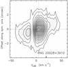 |
Fig. 22 Position-velocity diagram obtained along the symmetry axis at PA = 135° from the 12CO J = 1−0 line emission maps of IRAS 20028+3910. Contours are plotted at 2 and 5σ and from there with a spacing of 6σ, where σ = 15 mJy beam-1. |
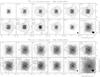 |
Fig. 23 Channel maps of the 12CO J = 1−0 and
J = 2−1 line emission toward IRAS 21282+5050 (in contours) at
the LSR velocities (units of km s-1) specified in the top-left corner
of each panel. No primary beam attenuation correction is applied. In the
background, in grey scale, the optical image obtained by (Sahai et al. 2007a) is shown for comparison.
(Top) CO J = 1−0: contours are plotted at
10, 20, and 40σ, and from there every 25σ, where
σ = 9.8 mJy beam-1. In the panels marked with
c in the bottom-left corner an additional contour is plotted at
4σ. Equivalent negative contours are plotted with dashed lines.
The last panel presents the continuum emission with a first contour and contour
spacing of 3σ, where
σ = 0.6 mJy beam-1. The synthesized beam, plotted in
the bottom-right corner of last panels, is |


The existing data for IRAS 23321+6545 are quite scarce. It is classified as a young PN from its cold FIR colors and broad CO emission (Volk & Kwok 1989; Bujarrabal et al. 2001). Radio continuum at mm wavelengths was previously detected by Walmsley et al. (1991), who concluded from extrapolation of FIR intensities that the detected flux is probably due to cold dust emission. IRAS 23321+6545 is very probably O-rich, since OH maser emission has been detected in it (Likkel, 1989). The source is very small in the optical and IR, tentatively showing a bipolar structure is the HST images (Ueta et al. 2000), elongated in the direction PA ≈ −45 degrees. We adopt the kinematical distance for vLSR = −55 km s-1, D = 4.5 kpc, which yields a reasonable total luminosity (Volk et al. 1993; Bujarrabal et al. 2001).
The PdBI observations of IRAS 23321+6545 were performed in track-sharing mode simultaneously with X Her (whose data are shown in Sect. 4.1.5). In addition, 30 m telescope observations were performed toward the source center. Other details about the observations and data reduction are given in Sect. 3 and in Table 2. The interferometric maps are shown in Fig. 24. The maps obtained for the central channels (marked with a “c” in the bottom-left corner), from −67 to −43 km s-1, are limited in the dynamic range, and therefore the lowest contour has not been plotted in those channels (more details can be found in the caption).
In Fig. 28 the spectra obtained for IRAS 23321+6545 are shown. The black solid line shows the integrated flux obtained for the CO lines from interferometric data. The dashed line shows the profile obtained with the 30 m telescope. Although IRAS 23321+6545 is found to be small, the contrast between single dish and interferometric integrated fluxes (Fig. 28) suggests the presence of an extended and tenuous halo filtered out by the PdBI.
Continuum is not detected at 2.6 mm with σ = 0.4 mJy, while it is detected at 1.3 mm at the 5.9σ level, where σ = 0.7 mJy (as can be seen in the last panel of Fig. 24). The position of the detection is however offset by ~0″̣5 with respect to the peak of the CO emission in the central channels of the maps displayed in Fig. 24, and coincides with the location of the redshifted emission. A better S/N detection would be needed in order to perform a better analysis.
Although the CO distribution in IRAS 23321+6545 (Fig. 24) is barely resolved, a significant characteristic is well revealed in these data. A position-velocity (P-V) gradient is detected along an axis with PA ≈ 90−95°. In Fig. 25 we show (on the left) the P-V diagram along an axis of PA = 93°, and (on the right) the CO J = 2−1 profile obtained at the central position. In both figures, an absorption at ~−70 km s-1 is present, which is similar to those seen in AFGL 2688 and IRAS 19500-1709 (Bujarrabal et al. 2001), AFGL 618 (Bujarrabal et al. 2001), IRAS 17436+5003 (Castro-Carrizo et al. 2004), and in this paper for IRAS 20028+3910 (Sect. 4.2.2), IK Tau (Sect. 4.1.2) and χ Cyg (Sect. 4.1.7). In all these cases we interpret this as absorption of the emission coming from excited innermost regions in the cooler outermost layers of the CSE closer to us. In well studied pPNe (Sánchez Contreras et al. 2004; Castro-Carrizo et al. 2004), these excited regions have been found to correspond to fast axial winds developing in the innermost layers of the large CSE shaped in the AGB phase. As seen in other cases (Sect. 4.2.2), this feature is not (not clearly at least) detected in the CO J = 1−0 emission, due to its relatively low opacity. Higher-resolution maps are needed for a deeper analysis of the axisymmetrical distribution in IRAS 23321+6545. This envelope seems to present fast axial winds in the innermost regions, interacting with outer layers of the envelope, as was concluded with a detailed modeling in AFGL 618 (Sánchez Contreras et al. 2004).
Finally, the profile obtained with the 30 m telescope (in dashed-line) shows an important ISM contribution between −28 and 5 km s-1, and at −85 km s-1 (Fig. 28). The interferometer filters out this extended contamination, and our compact emission is not much affected.
4.2.5. CRL 2477
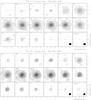 |
Fig. 24 Channel maps of the 12CO J = 1−0 and
J = 2−1 line emission toward IRAS 23321+6545 at the LSR
velocities (units of km s-1) specified in the top-left corner of each
panel. No primary beam attenuation correction is applied. (Top)
CO J = 1−0: contours are plotted from 3σ,
with a spacing of 3σ to 15σ, where
σ = 6.5 mJy beam-1. From 15σ
contours are plotted every 6σ. Equivalent negative contours are
plotted in dashed lines. The last panel presents the continuum emission with a
first contour and contour spacing of 3σ, where
σ = 0.4 mJy beam-1. The synthesized beam, plotted in
the bottom-right corner of last panels, is |

The nature of the poorly known source CRL 2477 is controversial. Volk et al. (1992) suggested that this source is in the post-AGB phase, mainly from its bimodal SED, due to the emission of both the central star and the nebular dust, which is characteristic of young PNe. Groenewegen & Whitelock (1996) argued, mainly because the stellar counterpart is O-rich while the nebular gas seems C-rich, that there are two stars coincident in the plane of the sky. Recent photometric observations (Kerschbaum et al. 2006) show that the bluest component, presumably the M-type star, is not variable, which may again support the post-AGB nature of CRL 2477.
CRL 2477 was observed at the PdBI in track-sharing mode with IRAS 19475+3119 (shown in Sect. 4.2.1). Considering the small angular size of the CSE as estimated by Neri et al. (1998), ≲ 6″, only observations at the central position were performed with the 30 m telescope. Other details about the observations and data calibration are given in Sect. 3 and in Table 2. Figure 26 presents the channel maps obtained with the interferometric data, no zero or short-spacing data are added.
In Fig. 28 we can see that the line profiles obtained with the single-dish (in dashed red lines) are significantly affected by ISM contamination. Since the profiles mainly present absorptions, a part of the ISM contribution may come from the off-source position (observed to subtract the baseline in the single-dish on-off observing mode; note that the obtained profile looks very similar to that obtained by Bujarrabal et al. 2001). In solid black lines, the profiles show the integrated fluxes derived from the interferometric maps (shown in Fig. 26). We can see that the interferometer filters out most of the ISM emission; we may have some ISM contribution in the channels with the most blueshifted emission for 12CO J = 2−1, but this is not clearly seen for the 12CO J = 1−0 maps and profile.
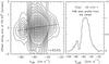 |
Fig. 25 Left: position-velocity diagram obtained along the symmetry axis at PA = 93° from the 12CO J = 2−1 line emission maps of IRAS 23321+6545. Right: CO J = 2−1 profile obtained at the central position (corresponding to a beam size). Contours are equivalent to those in Fig. 24. |
Continuum emission is detected at 1.3 mm at the J2000 coordinates RA 19:56:48.429, Dec 30:44:00.34 (J2000), which is the center of the maps shown in Fig. 26.
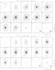 |
Fig. 26 Channel maps of the 12CO J = 1−0 and
J = 2−1 line emission toward CRL 2477 at the LSR velocities
(units of km s-1) specified in the top-left corner of each panel. No
primary beam attenuation correction is applied. (Top)
CO J = 1−0: contours are plotted from 3σ,
with a spacing of 4σ, where
σ = 7 mJy beam-1. Equivalent negative contours are
plotted in dashed lines. The last panel presents the continuum emission with a
first contour and contour spacing of 3σ, with
σ = 0.4 mJy beam-1. The synthesized beam, plotted in
the bottom-right corner of last panels, is |

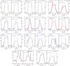 |
Fig. 27 Spectra resulting from integrating the 12CO J = 1−0 and J = 2−1 emissions in merged data maps in black solid lines, for the sources specified in the top-right corner. Red dotted lines show the profiles obtained by observing the source center with the 30 m telescope. The blue dashed lines show the integrated fluxes obtained from 30 m telescope OTF observations; they are displayed when they differ from the merged data fluxes due to primary beam attenuation effects (see Sect. 3). The zero level is dotted. For TX Cam, the red and black solid lines are different in the spectral resolution, the highest-resolution spectrum showing the ISM contamination close to 0 km s-1. See Sect. 4.1.6 for details about the CRL 2362 spectra. For OH 104.9+2.4 the data shown with black solid lines were obtained with the interferometer. |
The peaks in the channel-maps coincide with the continuum center. The emission centroids seem to be displaced a few fractions of an arcsecond toward the northeast however for many 12CO J = 2−1 channels. The J = 1−0 line emission is centered and peaks at the continuum position for most channels, but also shows a displacement at −8 km s-1 and +20 km s-1 consistent with that for the J = 2−1 emission. At −12 km s-1, mainly for the 12CO J = 1−0 maps, the emission is found to peak slightly toward the southwest. Note that the ISM contribution does not seem to be significant at this velocity (see Fig. 28). It is difficult to come to a conclusion about the nature of the above features and the evolutionary status of the source from our maps.
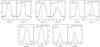 |
Fig. 28 Spectra resulting from integrating the 12CO J = 1−0 and J = 2−1 emissions in interferometric maps in black solid lines, for the sources specified in the top-right corner. Red dotted lines show the profiles obtained by observing the source center with the 30 m telescope. For IRAS 21282+5050 the data shown with black solid lines correspond to merged data maps, whose fluxes are similar to those from the OTF observations. The zero level is dotted. |
5. Discussion and conclusions
We present the first results of our COSAS program, a project to observe 12CO J = 1−0 and J = 2−1 line emission from AGB and post-AGB stars using the IRAM Plateau de Bure interferometer (PdBI) and the 30 m radiotelescope. We present the line emission maps of a sample of 16 objects out of a total sample of 45 sources (see Table 1). In most cases, 30 m telescope on-the-fly maps and PdBI high-resolution maps were merged to provide at the same time views of the structure of CSEs at small and large scales. Spatial resolutions as high as 1″ are reached in some sources. In the last two columns of Table 3 we summarize the main characteristics derived for this first subsample. A statistical study will be performed at the end of the publication of all the data, including more precise results from data modeling.
In general, the CSEs around AGB stars are found to show a roundish shape and more or less isotropic expansion. There is a stark contrast with the axial symmetry and fast bipolar flows found in most nebulae around post-AGB objects (pPNe and PNe). Nevertheless, in most AGB CSEs studied in this work, clear (though moderate) departures from spherical symmetry are found. We have mentioned a slight displacement westwards of the outermost regions of the CSE around IK Tau with respect to the position of the central region. The outermost regions of the CSEs of WX Psc and TX Cam show a clear elongation toward the northwest. The inner regions of IK Tau and χ Cyg show evidences of aspherical (relatively fast and excited) winds. In particular for χ Cyg this wind seems to expand at velocities moderately higher (by ≈ 5 km s-1) than those of the extended CSE.
The well-known more or less concentric arcs found in some AGB (and post-AGB) objects in scattered light images (Mauron & Huggins 2000, 2006), are also found in our data. Arcs are particularly evident in R Cas, for which we have been able to measure a typical separation of about 7″, corresponding to possible mass-loss-rate fluctuations over a time scale of ~350 yr. We clearly detect a similar feature in the inner CSEs around TX Cam. In this case (and perhaps also in R Cas) the structure seems to correspond to a spiral distribution rather than to concentric rings. This resembles the large spiral pattern seen in the optical in CRL 3068 (Mauron & Huggins 2006), possibly the effect of a binary companion.
Summary of source characteristics.
The two semiregular variables studied in this first subsample, X Her and RX Boo, show a clear axial symmetry and a velocity gradient along the axis in their CSE CO line emission. These features are more developed for X Her (which shows no trace of an outer rounded CSE) than for RX Boo (with a smaller axial distribution, surrounded by a large spherical CSE). Our maps suggest the presence of an hourglass-like structure and of an equatorial disk, similar to those seen in post-AGB sources like M 2-56 (Castro-Carrizo et al. 2002) and 89 Her (Bujarrabal et al. 2007), which are examples of sources with very different orientations with respect to the sky plane. At least in X Her, in which the central regions are quite well mapped, we can confirm that the equatorial disk is in slow expansion, at about 3 km s-1 (Sect. 4.5; Figs. 14, 15, and 44). No rotation is found in X Her; if it exists, the rotating gas must occupy a region smaller than 1″. The position-velocity diagram along the equatorial direction is found to be almost exactly symmetric with respect to both the spatial and velocity axes, very clearly different from the butterfly-like structure of Keplerian disks; our data show that the high-velocity components in this diagram are most probably due to emission from the faster hourglass-like component.
Note that the presence of hourglass-like outflows is found for the two SRs included in this paper. For another SR in our sample (which will be presented in a forthcoming paper), IRC+50049, our data also reveal the presence of axisymmetric mass loss. Moreover, similar axisymmetrical structures have been reported for other SR sources, e.g. V Hya (Kahane et al. 1996) and π1 Gru (Chiu et al. 2006a). For SRs, our sample is biased, since strong CO emitters (and hence sources with relatively large mass-loss rates) and some sources with peculiar line profiles (as in the case of X Her) were selected. Nevertheless, the results obtained for some of these objects (e.g. RX Boo and IRC +50049) were unexpected, considering previous information.
The CO CSEs detected around CRL 2362, OH 104.9+2.4 and CRL 2477 are too small and compact to easily allow an extraction of the CSE characteristics. Modeling the maps obtained for the two CO lines will allow us to determine additional mass-loss characteristics for these objects.
We have shown that two early post-AGB stars, IRAS 20028+3910 and IRAS 23321+6545, present fast axial winds confined within the slower spherical CSE, with which they interact. The position-velocity gradients observed along the symmetry axes traced by the fast components, the self absorption of part of the blue-shifted emission, and the contrast between the two CO lines support such a scenario.
We have also found a systematic feature in IRAS 20028+3910 and IRAS 23321+6545, which appear in similar sources like AFGL 2688 and IRAS 19500-1709 (Bujarrabal et al. 2001): the blue-shifted high-velocity component is significantly more prominent than the equivalent red-shifted component. In AFGL 618 (Bujarrabal et al. 2001) this characteristic is not observed. In other cases, like IRAS 17436+5003 (Castro-Carrizo et al. 2004), its presence is not clear. We argue that it is unlikely that these differences between the profile wings, so often found in pPNe, are simply due to mass differences between approaching and receding gas. Instead, we suggest that this phenomenon could be due to gas heating because of shock interaction between the fast collimated winds and the slower moving outer envelope (easier to detect when the fast component points towards the Earth). However, we cannot rule out that in some cases the effect appears as a consequence of an erroneous estimate of the systemic velocity, due to self absorption in the blue edge of the line profile.
IRAS 19475+3119 and IRAS 21282+5050 are post-AGB objects with more evolved nebulae (in the pPNe phase) than any other object in our subsample. The maps of IRAS 19475+3119 show a well developed circumstellar bipolar structure, whose lobes resemble those seen, for instance, in M 1-92 (Alcolea et al. 2007). For IRAS 21282+5050, an apparently very evolved structure with a big elongated hole at the center is found; axial winds may have created a cylinder-like structure in the innermost regions of this nebula.
Sizes measured at noise level in the 30 m telescope maps.
In most cases we see a large difference in size for the detected extent of halos in the CO J = 1−0 and J = 2−1 emissions. Sometimes this is clearly due to primary beam attenuation, which limits the extent of the mapped halo, see e.g. the maps and spectra obtained for R Cas and RX Boo, mainly for the J = 2−1 line, and TX Cam, χ Cyg and V Cyg in both lines. In other cases the mapping of the extended component becomes difficult due to the presence of strong side lobes, which happens mainly at 1.3 mm (e.g. for TX Cam, CRL 2362 and S Cep) or at both frequencies (IRAS 21282+5050). The J = 2−1 halo observations could be more limited than those of J = 1−0 due to the relative sensitivity. However, differences in the extent of the CO J = 2−1 and J = 1−0 emissions can also be due to differences in the line excitation conditions: the gas in the outermost regions is colder and less dense and hence more easily detectable in the CO J = 1−0 line. Detailed modeling of the excitation conditions is required to distinguish between these scenarios.
Independent estimates of the halo size can be made from the 30 m-telescope data. In Table 4, (beam convolved) total angular sizes at noise level measured from the 30 m telescope maps only are shown for those objects whose outermost emission is deduced to be attenuated by the PdBI primary beam. In the table we can also see estimates of the photodissociation diameters for AGB CSEs, from calculations by Mamon et al. (1988), using the parametrization by Loup et al. (1993); see Planesas et al. (1990). As we see, the total size of our mapped distribution, measured to noise level and including convolution with the 30 m telescope beam, are in general slightly larger than the expected total size of the CO-rich region. Although the comparison of both observational and theoretical results is in this case not straightforward, because it requires model calculations of the brightness distribution and beam convolution, we conclude that our high-sensitivity 30 m maps are not sensitivity-limited in general, and detect the total extent of the CO-rich envelope.
Maps of low-excitation CO lines are thought to provide a reliable image of the mass distribution in AGB and early post-AGB CSEs (see Sect. 1). However, CO photodissociation prevents the analysis of the outermost CSE regions from CO lines, which from a certain distance are not detected. We also note that an increase in the radiation field from one direction can yield a more efficient CO photodissociation in one side of the envelope, suggesting some asymmetry. We think that this effect should be in most cases easily differentiable from true axial symmetry.
Continuum fluxes obtained at 2.6 and 1.3 mm from the interferometric data.
In Table 5 we present the fluxes obtained for the continuum emission at 1.3 and 2.6 mm after subtracting the CO line emission. For comparison we also show IRAS fluxes at 12, 25, 60, and 100 μm obtained from the SIMBAD database. Continuum 30 m telescope observations in CW Leo by Groenewegen et al. (1997) show an emission extending ≳80″. This suggests that we filter out a large part of the CSE continuum emission in our data.
Online material
Observation summary.
Available in the IRAM’s web pages, Science Users section.
See IRAM’s web pages for a more updated view of the IRAM observatories.
See http://www.iram.fr/IRAMFR/GILDAS for more information about the GILDAS software package.
Acknowledgments
AC-C acknowledges financial support from the 6th European Community Framework Programme through a Marie-Curie Intra-European Fellowship. The contribution by GQ-L, V.B. and J.A. was supported by the Spanish Ministerio de Ciencia y Tecnologia and European FEDER funds, under grants AYA2000-0927, ESP2001-4519-PE and ESP2002-01693. F.L.S., H.O. and M.L. acknowledge financial support from the Swedish Research Council. We acknowledge the IRAM staff (both at Plateau de Bure and Grenoble) for carrying out the observations and the help they provided during the data reduction. We also acknowledge the GILDAS team for the many improvements carried out in the last years, either for the data reduction and analysis software. This research made use of the SIMBAD database, operated at CDS, Strasbourg, France, and of NASA’s Astrophysics Data System.
References
- Agúndez, M., & Cernicharo, J. 2006, ApJ, 650, 374 [NASA ADS] [CrossRef] [Google Scholar]
- Alcolea, J., Bujarrabal, V., Sánchez Contreras, C., Neri, R., & Zweigle, J. 2001, A&A, 373, 932 [NASA ADS] [CrossRef] [EDP Sciences] [Google Scholar]
- Alcolea, J., Neri, R., & Bujarrabal, V. 2007, A&A, 468, L41 [NASA ADS] [CrossRef] [EDP Sciences] [Google Scholar]
- Baars, J. W. M., Hooghoudt, B. G., Mezger, P. G., & de Jonge, M. J. 1987, A&A, 175, 319 [NASA ADS] [Google Scholar]
- Buemi, C. S., Umana, G., Trigilio, C., & Leto, P. 2007, A&A, 462, 637 [NASA ADS] [CrossRef] [EDP Sciences] [Google Scholar]
- Bujarrabal, V. 1999, in Asymptotic Giant Branch Stars, ed. T. Le Bertre, A. Lebre, & C. Waelkens, IAU Symp., 191, 363 [Google Scholar]
- Bujarrabal, V., Alcolea, J., & Neri, R. 1998, ApJ, 504, 915 [NASA ADS] [CrossRef] [Google Scholar]
- Bujarrabal, V., Castro-Carrizo, A., Alcolea, J., & Sánchez Contreras, C. 2001, A&A, 377, 868 [NASA ADS] [CrossRef] [EDP Sciences] [Google Scholar]
- Bujarrabal, V., van Winckel, H., Neri, R., et al. 2007, A&A, 468, L45 [NASA ADS] [CrossRef] [EDP Sciences] [Google Scholar]
- Castro-Carrizo, A., Bujarrabal, V., Sánchez Contreras, C., Alcolea, J., & Neri, R. 2002, A&A, 386, 633 [NASA ADS] [CrossRef] [EDP Sciences] [Google Scholar]
- Castro-Carrizo, A., Neri, R., & Winters, J. M. 2004, in Asymmetrical Planetary Nebulae III: Winds, Structure and the Thunderbird, ed. M. Meixner, J. H. Kastner, B. Balick, & N. Soker, ASP Conf. Ser., 313, 314 [Google Scholar]
- Castro-Carrizo, A., Neri, R., Winters, J. M., et al. 2007, in Why Galaxies Care About AGB Stars: Their Importance as Actors and Probes, ed. F. Kerschbaum, C. Charbonnel, & R. F. Wing, ASP Conf. Ser., 378, 199 [Google Scholar]
- Cherchneff, I. 2006, A&A, 456, 1001 [NASA ADS] [CrossRef] [EDP Sciences] [Google Scholar]
- Chiu, P., Hoang, C., Dinh-V-Trung, et al. 2006a, ApJ, 645, 605 [NASA ADS] [CrossRef] [Google Scholar]
- Chiu, P.-J., Hoang, C.-T., Dinh-V-Trung, et al. 2006b, ApJ, 645, 605 [NASA ADS] [CrossRef] [Google Scholar]
- Cox, P., Lucas, R., Huggins, P. J., et al. 2000, A&A, 353, L25 [NASA ADS] [Google Scholar]
- Crowther, P. A., De Marco, O., & Barlow, M. J. 1998, MNRAS, 296, 367 [Google Scholar]
- Dinh-V.-Trung, & Lim, J. 2009, ApJ, 701, 292 [NASA ADS] [CrossRef] [Google Scholar]
- Feast, M. W., Glass, I. S., Whitelock, P. A., & Catchpole, R. M. 1989, MNRAS, 241, 375 [NASA ADS] [CrossRef] [Google Scholar]
- Fong, D., Meixner, M., & Shah, R. Y. 2003, ApJ, 582, L39 [NASA ADS] [CrossRef] [Google Scholar]
- Fong, D., Meixner, M., Sutton, E. C., Zalucha, A., & Welch, W. J. 2006, ApJ, 652, 1626 [NASA ADS] [CrossRef] [Google Scholar]
- Gardan, E., Gérard, E., & Le Bertre, T. 2006, MNRAS, 365, 245 [NASA ADS] [CrossRef] [Google Scholar]
- Gledhill, T. M., Chrysostomou, A., Hough, J. H., & Yates, J. A. 2001, MNRAS, 322, 321 [NASA ADS] [CrossRef] [Google Scholar]
- González Delgado, D., Olofsson, H., Kerschbaum, F., et al. 2003, A&A, 411, 123 [NASA ADS] [CrossRef] [EDP Sciences] [Google Scholar]
- Groenewegen, M. A. T., & Whitelock, P. A. 1996, MNRAS, 281, 1347 [NASA ADS] [CrossRef] [Google Scholar]
- Groenewegen, M. A. T., Oudmaijer, R. D., Goudfrooij, P., van den Hoek, L. B., & van Kerkwijk, M. H. 1996, A&A, 305, 475 [NASA ADS] [Google Scholar]
- Groenewegen, M. A. T., van der Veen, W. E. C. J., Lefloch, B., & Omont, A. 1997, A&A, 322, L21 [NASA ADS] [Google Scholar]
- Guélin, M., Lucas, R., Neri, R., Bremer, M., & Broguiere, D. 2000, in From Molecular Clouds to Planetary, ed. Y. C. Minh, & E. F. van Dishoeck, IAU Symp., 197, 365 [Google Scholar]
- Guilloteau, S., Delannoy, J., Downes, D., et al. 1992, A&A, 262, 624 [NASA ADS] [Google Scholar]
- Heske, A., Forveille, T., Omont, A., van der Veen, W. E. C. J., & Habing, H. J. 1990, A&A, 239, 173 [NASA ADS] [Google Scholar]
- Hirano, N., Shinnaga, H., Dinh-V-Trung, et al. 2004, ApJ, 616, L43 [NASA ADS] [CrossRef] [Google Scholar]
- Högbom, J. A. 1974, A&AS, 15, 417 [Google Scholar]
- Hrivnak, B. J., & Bieging, J. H. 2005, ApJ, 624, 331 [NASA ADS] [CrossRef] [Google Scholar]
- Hrivnak, B. J., Geballe, T. R., & Kwok, S. 2007, ApJ, 662, 1059 [NASA ADS] [CrossRef] [Google Scholar]
- Hrivnak, B. J., Kwok, S., & Su, K. Y. L. 2001, AJ, 121, 2775 [NASA ADS] [CrossRef] [Google Scholar]
- Kahane, C., & Jura, M. 1996, A&A, 310, 952 [NASA ADS] [Google Scholar]
- Kahane, C., Audinos, P., Barnbaum, C., & Morris, M. 1996, A&A, 314, 871 [NASA ADS] [Google Scholar]
- Kerschbaum, F., & Olofsson, H. 1999, A&AS, 138, 299 [NASA ADS] [CrossRef] [EDP Sciences] [Google Scholar]
- Kerschbaum, F., Groenewegen, M. A. T., & Lazaro, C. 2006, A&A, 460, 539 [NASA ADS] [CrossRef] [EDP Sciences] [Google Scholar]
- Kholopov, P. N., Samus, N. N., Frolov, M. S., et al. 1999, VizieR Online Data Catalog, 2214, [Google Scholar]
- Knapp, G. R., Young, K., Lee, E., & Jorissen, A. 1998, ApJS, 117, 209 [NASA ADS] [CrossRef] [Google Scholar]
- Likkel, L., Morris, M., Forveille, T., & Omont, A. 1988, A&A, 198, L1 [NASA ADS] [Google Scholar]
- Likkel, L., Morris, M., Kastner, J. H., & Forveille, T. 1994, A&A, 282, 190 [NASA ADS] [Google Scholar]
- Likkel, L., Morris, M., Omont, A., & Forveille, T. 1987, A&A, 173, L11 [NASA ADS] [Google Scholar]
- Lindqvist, M., Nyman, L.-Å., Olofsson, H., & Winnberg, A. 1988, A&A, 205, L15 [NASA ADS] [Google Scholar]
- Lindqvist, M., Olofsson, H., Lucas, R., et al. 1999, A&A, 351, L1 [NASA ADS] [Google Scholar]
- Loup, C., Forveille, T., Omont, A., & Paul, J. F. 1993, A&AS, 99, 291 [NASA ADS] [Google Scholar]
- Maercker, M. 2010, Ph.D. Thesis, Stockholm University [Google Scholar]
- Maercker, M., Schöier, F. L., Olofsson, H., Bergman, P., & Ramstedt, S. 2008, A&A, 479, 779 [NASA ADS] [CrossRef] [EDP Sciences] [Google Scholar]
- Mamon, G. A., Glassgold, A. E., & Huggins, P. J. 1988, ApJ, 328, 797 [NASA ADS] [CrossRef] [Google Scholar]
- Mattsson, L., Höfner, S., & Herwig, F. 2007, A&A, 470, 339 [NASA ADS] [CrossRef] [EDP Sciences] [Google Scholar]
- Mauron, N., & Huggins, P. J. 1999, A&A, 349, 203 [NASA ADS] [Google Scholar]
- Mauron, N., & Huggins, P. J. 2000, A&A, 359, 707 [NASA ADS] [Google Scholar]
- Mauron, N., & Huggins, P. J. 2006, A&A, 452, 257 [NASA ADS] [CrossRef] [EDP Sciences] [Google Scholar]
- Meixner, M., Skinner, C. J., Graham, J. R., et al. 1997, ApJ, 482, 897 [NASA ADS] [CrossRef] [Google Scholar]
- Meixner, M., Campbell, M. T., Welch, W. J., & Likkel, L. 1998, ApJ, 509, 392 [NASA ADS] [CrossRef] [Google Scholar]
- Myasnikov, A. V., Belov, N. A., Gustafsson, B., & Eriksson, K. 2000, Ap&SS, 274, 231 [NASA ADS] [CrossRef] [Google Scholar]
- Nakashima, J.-i. 2005, ApJ, 620, 943 [NASA ADS] [CrossRef] [Google Scholar]
- Nakashima, J.-i. 2006, ApJ, 638, 1041 [NASA ADS] [CrossRef] [Google Scholar]
- Neri, R., Kahane, C., Lucas, R., Bujarrabal, V., & Loup, C. 1998, A&AS, 130, 1 [NASA ADS] [CrossRef] [EDP Sciences] [Google Scholar]
- Olofsson, H., Carlstrom, U., Eriksson, K., Gustafsson, B., & Willson, L. A. 1990, A&A, 230, L13 [NASA ADS] [Google Scholar]
- Olofsson, H., Bergman, P., Eriksson, K., & Gustafsson, B. 1996, A&A, 311, 587 [NASA ADS] [Google Scholar]
- Olofsson, H., Bergman, P., Lucas, R., et al. 2000, A&A, 353, 583 [NASA ADS] [Google Scholar]
- Olofsson, H., González Delgado, D., Kerschbaum, F., & Schöier, F. L. 2002, A&A, 391, 1053 [NASA ADS] [CrossRef] [EDP Sciences] [Google Scholar]
- Planesas, P., Bachiller, R., Martin-Pintado, J., & Bujarrabal, V. 1990, ApJ, 351, 263 [NASA ADS] [CrossRef] [Google Scholar]
- Ramstedt, S., Schöier, F. L., Olofsson, H., & Lundgren, A. A. 2006, A&A, 454, L103 [NASA ADS] [CrossRef] [EDP Sciences] [Google Scholar]
- Ramstedt, S., Schöier, F. L., Olofsson, H., & Lundgren, A. A. 2008, A&A, 487, 645 [NASA ADS] [CrossRef] [EDP Sciences] [Google Scholar]
- Ramstedt, S., Schöier, F. L., & Olofsson, H. 2009, A&A, 499, 515 [NASA ADS] [CrossRef] [EDP Sciences] [Google Scholar]
- Sahai, R., Morris, M., Sánchez Contreras, C., & Claussen, M. 2007a, AJ, 134, 2200 [NASA ADS] [CrossRef] [Google Scholar]
- Sahai, R., Sánchez Contreras, C., Morris, M., & Claussen, M. 2007b, ApJ, 658, 410 [NASA ADS] [CrossRef] [Google Scholar]
- Samus, N. N., Durlevich, O. V., et al. 2004, VizieR Online Data Catalog, 2250 [Google Scholar]
- Sánchez Contreras, C., Bujarrabal, V., Castro-Carrizo, A., Alcolea, J., & Sargent, A. 2004, ApJ, 617, 1142 [NASA ADS] [CrossRef] [Google Scholar]
- Sánchez Contreras, C., Bujarrabal, V., Castro-Carrizo, A., Alcolea, J., & Sargent, A. 2006, ApJ, 643, 945 [NASA ADS] [CrossRef] [Google Scholar]
- Sarkar, G., & Sahai, R. 2006, ApJ, 644, 1171 [NASA ADS] [CrossRef] [Google Scholar]
- Schöier, F. L., & Olofsson, H. 2001, A&A, 368, 969 [NASA ADS] [CrossRef] [EDP Sciences] [Google Scholar]
- Schöier, F. L., Olofsson, H., Wong, T., Lindqvist, M., & Kerschbaum, F. 2004, A&A, 422, 651 [NASA ADS] [CrossRef] [EDP Sciences] [Google Scholar]
- Schöier, F. L., Lindqvist, M., & Olofsson, H. 2005, A&A, 436, 633 [NASA ADS] [CrossRef] [EDP Sciences] [Google Scholar]
- Schöier, F. L., Fong, D., Olofsson, H., Zhang, Q., & Patel, N. 2006a, ApJ, 649, 965 [NASA ADS] [CrossRef] [Google Scholar]
- Schöier, F. L., Olofsson, H., & Lundgren, A. A. 2006b, A&A, 454, 247 [NASA ADS] [CrossRef] [EDP Sciences] [Google Scholar]
- Sedlmayr, E. 1994, in Molecules in the Stellar Environment, ed. U. G. Jorgensen, Lecture Notes in Physics 428 (Berlin Springer Verlag), IAU Colloq., 146, 163 [Google Scholar]
- Silverglate, P., Terzian, Y., Zuckerman, B., & Wolff, M. 1979, AJ, 84, 345 [NASA ADS] [CrossRef] [Google Scholar]
- Steer, D. G., Dewdney, P. E., & Ito, M. R. 1984, A&A, 137, 159 [NASA ADS] [Google Scholar]
- Steffen, M., & Schönberner, D. 2000, A&A, 357, 180 [NASA ADS] [Google Scholar]
- Su, K. Y. L., Hrivnak, B. J., & Kwok, S. 2001, AJ, 122, 1525 [NASA ADS] [CrossRef] [Google Scholar]
- Teyssier, D., Hernandez, R., Bujarrabal, V., Yoshida, H., & Phillips, T. G. 2006, A&A, 450, 167 [NASA ADS] [CrossRef] [EDP Sciences] [Google Scholar]
- Ueta, T., Meixner, M., & Bobrowsky, M. 2000, ApJ, 528, 861 [NASA ADS] [CrossRef] [Google Scholar]
- van Langevelde, H. J., Janssens, A. M., Goss, W. M., Habing, H. J., & Winnberg, A. 1993, A&AS, 101, 109 [Google Scholar]
- Volk, K. M., & Kwok, S. 1989, ApJ, 342, 345 [NASA ADS] [CrossRef] [Google Scholar]
- Volk, K., Kwok, S., & Langill, P. P. 1992, ApJ, 391, 285 [NASA ADS] [CrossRef] [Google Scholar]
- Volk, K., Kwok, S., & Woodsworth, A. W. 1993, ApJ, 402, 292 [NASA ADS] [CrossRef] [Google Scholar]
- Walmsley, C. M., Chini, R., Kreysa, E., et al. 1991, A&A, 248, 555 [NASA ADS] [Google Scholar]
- Whitelock, P., Menzies, J., Feast, M., et al. 1994, MNRAS, 267, 711 [NASA ADS] [CrossRef] [Google Scholar]
All Tables
All Figures
|
Fig. 1 Channel maps of the 12CO J = 1−0 and
J = 2−1 line emission towards WX Psc. The maps are corrected
for primary beam attenuation. The LSR velocities (units of km s-1) are
shown in the top-left corner of each panel. (Top) CO
J = 1−0: contours start at 4σ and are in steps
of 5σ with σ = 22 mJy beam-1. Negative
contours are plotted with the same spacing in dashed lines. The last panel shows the
continuum emission with a contour spacing of 2σ and
σ = 1.6 mJy beam-1. The synthesized beam is
|
| In the text | |
|
Fig. 2 Channel maps of the 12CO J = 1−0 and
J = 2−1 line emission towards IK Tau. The maps are corrected
for primary beam attenuation. The LSR velocities (units of km s-1) are
shown in the top-left corner of each panel. (Top) CO
J = 1−0: contours start at 4σ and are in
steps of 6σ with σ = 21 mJy beam-1.
Equivalent negative contours are plotted in dashed lines. The last panel shows the
continuum emission with a first contour and contour spacing of 3σ
and σ = 0.87 mJy beam-1. The synthesized beam is
|
| In the text | |
|
Fig. 3 Channel maps of the 12CO J = 2−1 line emission towards IK Tau with a spectral resolution of 2 km s-1. The LSR velocities (units of km s-1) are given in the top-left corner of each panel. Contours are plotted with a first contour and contour spacing of 4σ and σ = 45 mJy beam-1. The map center coordinates are RA 03:53:28.907, Dec 11:24:21.84 (J2000). |
| In the text | |
|
Fig. 4 Spectra observed towards the center of IK Tau and χ Cyg (solid lines) and obtained by spatially integrating over the emission regions (dashed lines). The latter are shown scaled for comparison. The widths at zero-power of the J = 2−1 and J = 1−0 lines appear to be similar for IK Tau. Self-absorption is well detected in the CSEs of both stars, i.e., blueshifted J = 2−1 emission from warm gas in the inner CSE regions is partly absorbed in the outer layers. In χ Cyg small wings are detected at zero-power in the J = 2−1 line. |
| In the text | |
|
Fig. 5 Channel maps of the
12CO J = 1−0 and J = 2−1 line
emission towards TX Cam. The LSR velocities (units of km s-1) are shown
in the top-left corner of each panel. No primary beam attenuation correction is
applied. (Top) CO J = 1−0: contours are
plotted for 3, 7, 11, 23, and 35σ, and from there with a spacing
of 21σ and with σ = 9.6 mJy beam-1.
In the channels labeled “c” in the bottom-left corner, contours at 15 and
19σ are also plotted. Negative contours are dashed and start at
−3σ. The panel in the bottom-right corner shows the continuum
emission with contours starting at 3σ, in steps of
6σ, with σ = 0.54 mJy beam-1. The
synthesized beam is |
| In the text | |
|
Fig. 6 Composite image of TX Cam overlaying the 12CO J = 1−0 emission in the outermost regions (black contours) and the 12CO J = 2−1 emission from the interferometric data alone (red contours). Interferometric data alone provide a more genuine rendition of the innermost structure. The synthesized beams of both datasets are plotted in the bottom-right corner. |
| In the text | |
|
Fig. 7 Channel maps of the 12CO J = 1−0 and
J = 2−1 line emission towards RX Boo. The LSR velocities
(units of km s-1) are shown in the top-left corner of each panel. No
primary beam attenuation correction is applied. (Top) CO
J = 1−0: contours are plotted from 3σ in
steps of 3σ with σ = 16 mJy beam-1.
Equivalent negative contours are plotted with dashed lines. The last panel shows
the continuum emission with contours starting at 3σ in steps of
3σ with σ = 0.6 mJy beam-1, and the
synthesized beam in the bottom-right corner of size |
| In the text | |
|
Fig. 8 Position-velocity diagram along the symmetry axis, at PA = 50°, of the 12CO J = 1−0 emission maps towards RX Boo. Contours are equivalent to those shown in Fig. 7. |
| In the text | |
|
Fig. 9 Channel maps of the 12CO J = 1−0 and
J = 2−1 line emission towards X Her, at the LSR velocities
(units of km s-1) specified in the top-left corner of each panel. No
primary beam attenuation correction is applied. (Top) CO
J = 1−0: contours are plotted from and with a spacing of
2.5σ, where σ = 10 mJy beam-1.
Equivalent negative contours are plotted in dashed lines. The last panel presents
the continuum emission from and with a spacing of 2.5σ, with
σ = 0.35 mJy beam-1. The synthesized beam is
|
| In the text | |
|
Fig. 10 (Left): position-velocity diagram along the symmetry axis at PA = 45° of the 12CO J = 1−0 emission towards X Her. (Right): the same along an axis at PA = −45°. Contours are equivalent to those shown in Fig. 9. |
| In the text | |
|
Fig. 11 Channel maps of the 12CO J = 1−0 and
J = 2−1 emission toward CRL 2362 at the LSR velocities (units
of km s-1) specified in the top-left corner of each panel. No primary
beam attenuation correction is applied. (Top) CO
J = 1−0: contours are plotted from and with a spacing of
3σ, where σ = 7 mJy beam-1.
Negative contours are plotted in dashed lines with the same spacing. The last
panel presents the continuum emission with a first contour and contour spacing of
3σ, with σ = 0.3 mJy beam-1. The
synthesized beam is |
| In the text | |
|
Fig. 12 Channel maps of the 12CO J = 1−0 and
J = 2−1 line emission toward χ Cyg at the
LSR velocities (units of km s-1) specified in the top-left corner of
each panel. No primary beam attenuation correction is applied.
(Top) CO J = 1−0: contours are plotted from
4σ, with a spacing of 8σ, where
σ = 10 mJy beam-1. In the panels marked with
c in the bottom-left corner the first four contours are at 4,
12, 20 and 28σ, and from there the spacing is
20σ. Equivalent negative contours are plotted in dashed lines.
The last channel presents the continuum emission with a first contour and contour
spacing of 3 and 6σ respectively, where
σ = 0.4 mJy beam-1. The synthesized beam, plotted in
the bottom-right corner of last panels, is |
| In the text | |
|
Fig. 13 Some channel maps obtained for the CO J = 1−0 (upper) and J = 2−1 (lower) emission toward χ Cyg with 1 km s-1 spectral resolution (LSR velocities specified in the top-left corner of each channel, in km s-1). In the J = 1−0 channel maps, contours are plotted from 3σ, with a spacing of 6σ, with σ = 14 mJy beam-1. In the J = 2−1 channel maps, contours are plotted from 4σ, with a spacing of 6σ, with σ = 30 mJy beam-1. |
| In the text | |
|
Fig. 14 Channel maps of the 12CO J = 1−0 and
J = 2−1 line emission toward V Cyg at the LSR velocities
(units of km s-1) specified in the top-left corner of each panel. No
primary beam attenuation correction is applied. (Top) CO
J = 1−0: contours are plotted at 5, 12, 24, and
42σ and from there with a spacing of 20σ,
where σ = 7.8 mJy beam-1. Equivalent negative
contours are plotted in dashed lines. The last panel presents the continuum
emission with a first contour and contour spacing of 3σ, where
σ = 0.4 mJy beam-1. The synthesized beam, plotted in
the bottom-right corner of last panels, is |
| In the text | |
|
Fig. 15 Channel maps of the 12CO J = 1−0 and J = 2−1 line emission toward S Cep at the LSR velocities (units of km s-1) specified in the top-left corner of each panel. No primary beam attenuation correction is applied. (Top) CO J = 1−0: contours are plotted at 3, 6, 9, and 12σ, and from there with a spacing of 10σ, where σ = 7.9 mJy beam-1. Equivalent negative contours are plotted in dashed lines. The last panel presents the continuum emission with a first contour and contour spacing of 3σ, where σ = 0.6 mJy beam-1. The synthesized beam, plotted in the bottom-right corner of last panels, is 3″̣3 × 2″̣8 in size, with PA = 21°. (Bottom) CO J = 2−1: contours are plotted from and with a spacing of 6σ, where σ = 18 mJy beam-1. In the panels marked with c in the bottom-left corner, from the contour at 24σ the spacing is 12σ. Equivalent negative contours are plotted in dashed lines. The last panel presents the continuum emission with a first contour and contour spacing of 3σ, where σ = 1.4 mJy beam-1. The synthesized beam, plotted in the bottom-right corner of last panels, is 1″̣7 × 1″̣3 in size, with PA = 27°. The primary beams are plotted at half power in dotted lines in the last panels of the channel maps. The central coordinates are RA 21:35:12.830, Dec 78:37:28.19 (J2000). |
| In the text | |
|
Fig. 16 Channel maps of
the 12CO J = 1−0 and J = 2−1 line
emission toward OH 104.9+2.4 at the LSR velocities (units of km s-1)
specified in the top-left corner of each panel. No primary beam attenuation
correction is applied. (Top) CO J = 1−0:
contours are plotted from, and with a spacing of, 0.032 Jy beam-1.
Equivalent negative contours are plotted in dashed lines. The last panel presents
the continuum emission with a first contour and contour spacing of
3σ, where σ = 0.65 mJy beam-1. The
synthesized beam, plotted in the bottom-right corner of last panels, is
|
| In the text | |
|
Fig. 17 Channel maps of the
12CO J = 1−0 and J = 2−1 line
emission toward R Cas at the LSR velocities (units of km s-1) specified
in the top-left corner of each panel. No primary beam attenuation correction is
applied. (Top) CO J = 1−0: contours are
plotted from 3σ and from there with a spacing of
3σ, where σ = 11mJy beam-1.
Equivalent negative contours are plotted in dashed lines. The last panel presents
the continuum emission with a first contour and contour spacing of
4σ, where σ = 0.6 mJy beam-1. The
synthesized beam, plotted in the bottom-right corner of last panels, is
|
| In the text | |
|
Fig. 18 (Left:) channel maps of the 12CO J = 2−1 line emission toward R Cas equivalent to those shown in Fig. 17, resulting from CLEANing with the SDI method. Contours are plotted at 3.5, 7, 10.5, 14, 19 and 24σ and from there each 8σ, where σ = 29 mJy beam-1. Although the results obtained with different CLEANing methods allow emphasizing different structures, the resulted brightness distributions are very compatible. (Right:) the azimuthal average of the brightness distribution around the center is shown, at the systemic velocity (25 km s-1), for both 12CO J = 1−0 and J = 2−1 emission. Peaks are found at the same radius for both transitions. |
| In the text | |
|
Fig. 19 Channel maps of the 12CO J = 1−0 and
J = 2−1 emissions (in contours) toward IRAS 19475+3119 at the
LSR velocities (units of km s-1) specified in the top-left corner of
each panel. In the background, in grey scale, the optical image obtained by (Sahai et al. 2007b) is shown for comparison. No
primary beam attenuation correction is applied. (Top)
CO J = 1−0: contours are plotted from and with a spacing of
2.8σ, where σ = 6.9 mJy beam-1.
Equivalent negative contours are plotted with dashed lines. Contours presenting
relative minima in the CSE are plotted in grey (red in the electronic version).
The synthesized beam is |
| In the text | |
|
Fig. 20 Left: position-velocity diagram along the symmetry axis at PA = 90° of the 12CO J = 2−1 emission maps towards IRAS 19475+3119. Contours are plotted from 2σ with the same spacing. Right: the same along an axis at PA = 0°. Contours are plotted from 6σ, with a spacing of 3σ (σ = 11 mJy beam-1). |
| In the text | |
|
Fig. 21 Channel maps of the 12CO J = 1−0 and
J = 2−1 line emission (in contours) toward IRAS 20028+3910 at
the LSR velocities (units of km s-1) specified in the top-left corner
of each panel. No primary beam attenuation correction is applied.
(Top) CO J = 1−0: contours are superposed on
HST images by Ueta et al. (2000), and
plotted from 2.6σ, with a spacing of 3σ, where
σ = 7.1 mJy beam-1. In the panels marked with
c in the bottom-left corner the first contours are at 6, 10,
15, 21, 27, 34σ and from there every 15σ.
Equivalent negative contours are plotted in dashed lines. The last panel presents
the continuum emission with a first contour and contour spacing of
3σ, where σ = 0.5 mJy beam-1. The
synthesized beam, plotted in the bottom-right corner of last panels, is
|
| In the text | |
|
Fig. 22 Position-velocity diagram obtained along the symmetry axis at PA = 135° from the 12CO J = 1−0 line emission maps of IRAS 20028+3910. Contours are plotted at 2 and 5σ and from there with a spacing of 6σ, where σ = 15 mJy beam-1. |
| In the text | |
|
Fig. 23 Channel maps of the 12CO J = 1−0 and
J = 2−1 line emission toward IRAS 21282+5050 (in contours) at
the LSR velocities (units of km s-1) specified in the top-left corner
of each panel. No primary beam attenuation correction is applied. In the
background, in grey scale, the optical image obtained by (Sahai et al. 2007a) is shown for comparison.
(Top) CO J = 1−0: contours are plotted at
10, 20, and 40σ, and from there every 25σ, where
σ = 9.8 mJy beam-1. In the panels marked with
c in the bottom-left corner an additional contour is plotted at
4σ. Equivalent negative contours are plotted with dashed lines.
The last panel presents the continuum emission with a first contour and contour
spacing of 3σ, where
σ = 0.6 mJy beam-1. The synthesized beam, plotted in
the bottom-right corner of last panels, is |
| In the text | |
|
Fig. 24 Channel maps of the 12CO J = 1−0 and
J = 2−1 line emission toward IRAS 23321+6545 at the LSR
velocities (units of km s-1) specified in the top-left corner of each
panel. No primary beam attenuation correction is applied. (Top)
CO J = 1−0: contours are plotted from 3σ,
with a spacing of 3σ to 15σ, where
σ = 6.5 mJy beam-1. From 15σ
contours are plotted every 6σ. Equivalent negative contours are
plotted in dashed lines. The last panel presents the continuum emission with a
first contour and contour spacing of 3σ, where
σ = 0.4 mJy beam-1. The synthesized beam, plotted in
the bottom-right corner of last panels, is |
| In the text | |
|
Fig. 25 Left: position-velocity diagram obtained along the symmetry axis at PA = 93° from the 12CO J = 2−1 line emission maps of IRAS 23321+6545. Right: CO J = 2−1 profile obtained at the central position (corresponding to a beam size). Contours are equivalent to those in Fig. 24. |
| In the text | |
|
Fig. 26 Channel maps of the 12CO J = 1−0 and
J = 2−1 line emission toward CRL 2477 at the LSR velocities
(units of km s-1) specified in the top-left corner of each panel. No
primary beam attenuation correction is applied. (Top)
CO J = 1−0: contours are plotted from 3σ,
with a spacing of 4σ, where
σ = 7 mJy beam-1. Equivalent negative contours are
plotted in dashed lines. The last panel presents the continuum emission with a
first contour and contour spacing of 3σ, with
σ = 0.4 mJy beam-1. The synthesized beam, plotted in
the bottom-right corner of last panels, is |
| In the text | |
|
Fig. 27 Spectra resulting from integrating the 12CO J = 1−0 and J = 2−1 emissions in merged data maps in black solid lines, for the sources specified in the top-right corner. Red dotted lines show the profiles obtained by observing the source center with the 30 m telescope. The blue dashed lines show the integrated fluxes obtained from 30 m telescope OTF observations; they are displayed when they differ from the merged data fluxes due to primary beam attenuation effects (see Sect. 3). The zero level is dotted. For TX Cam, the red and black solid lines are different in the spectral resolution, the highest-resolution spectrum showing the ISM contamination close to 0 km s-1. See Sect. 4.1.6 for details about the CRL 2362 spectra. For OH 104.9+2.4 the data shown with black solid lines were obtained with the interferometer. |
| In the text | |
|
Fig. 28 Spectra resulting from integrating the 12CO J = 1−0 and J = 2−1 emissions in interferometric maps in black solid lines, for the sources specified in the top-right corner. Red dotted lines show the profiles obtained by observing the source center with the 30 m telescope. For IRAS 21282+5050 the data shown with black solid lines correspond to merged data maps, whose fluxes are similar to those from the OTF observations. The zero level is dotted. |
| In the text | |
Current usage metrics show cumulative count of Article Views (full-text article views including HTML views, PDF and ePub downloads, according to the available data) and Abstracts Views on Vision4Press platform.
Data correspond to usage on the plateform after 2015. The current usage metrics is available 48-96 hours after online publication and is updated daily on week days.
Initial download of the metrics may take a while.