| Issue |
A&A
Volume 709, May 2026
|
|
|---|---|---|
| Article Number | A143 | |
| Number of page(s) | 19 | |
| Section | Interstellar and circumstellar matter | |
| DOI | https://doi.org/10.1051/0004-6361/202659537 | |
| Published online | 12 May 2026 | |
The dusty envelopes of asymptotic giant branch stars with ultraviolet excesses
1
Centro de Astrobiología, CSIC-INTA,
Camino bajo del Castillo s/n,
28692
Villanueva de la Cañada,
Madrid,
Spain
2
Escuela de Doctorado UAM, Centro de Estudios de Posgrado, Universidad Autónoma de Madrid,
28049
Madrid,
Spain
3
Jet Propulsion Laboratory, California Institute of Technology,
Pasadena,
CA
91109,
USA
★ Corresponding author: This email address is being protected from spambots. You need JavaScript enabled to view it.
Received:
20
February
2026
Accepted:
19
March
2026
Abstract
Context. Roughly spherical envelopes around asymptotic giant branch (AGB) stars transform into the highly asymmetric morphologies observed in planetary nebulae. The complex processes involved in this metamorphosis are not yet completely understood. However, binarity emerges as a strong shaping factor, although the identification of binary companions in AGB stars is observationally challenging. The presence of ultraviolet (UV) excesses in AGB stars has been suggested as a potential indicator of binarity.
Aims. In a first study, we characterised the properties of the gas component in the circumstellar envelopes surrounding a sample of 29 AGB stars with UV excesses. Now, we intend to complement this information with an analysis of the dust component and compare the estimated parameters with those previously inferred from larger samples of AGB stars.
Methods. We modelled the spectral energy distributions of the sample using dust radiative transfer models. In some cases, we complemented the analysis with Herschel/PACS radial surface brightness profiles.
Results. We derived mass-loss rates and gas-to-dust ratios, which are in the typical ranges for AGB stars. We found that the stellar and mass-loss parameters follow similar trends to those presented in the literature. There is an anticorrelation between the gas-to-dust ratio and the UV emission, although it is weaker than its correlations with pulsation and mass-loss. We also estimated the dust attenuation produced by the dust at UV wavelengths and describe its effects on the intrinsic UV emission.
Conclusions. Stellar and mass-loss parameters of UV emitting AGB stars follow similar trends as found for larger samples of AGB stars. High-angular-resolution observations are required to explore the dust-forming regions and identify the presence of stellar companions. Circumstellar dust attenuation might play a dominant role in the observed UV emission and needs to be taken into account to estimate the intrinsic UV emission.
Key words: stars: AGB and post-AGB / circumstellar matter / stars: mass-loss / dust, extinction / ultraviolet: stars
© The Authors 2026
 Open Access article, published by EDP Sciences, under the terms of the Creative Commons Attribution License (https://creativecommons.org/licenses/by/4.0), which permits unrestricted use, distribution, and reproduction in any medium, provided the original work is properly cited.
This article is published in open access under the Subscribe to Open model. This email address is being protected from spambots. You need JavaScript enabled to view it. to support open access publication.
1 Introduction
When stars with low and intermediate masses (i.e. with masses ~1-8 M⊙) leave the main sequence, they evolve through the Hertzsprung-Russell diagram (HRD), increasing their luminosities while lowering their effective temperatures. They eventually reach the asymptotic giant branch (AGB). At this stage their huge luminosities (from hundreds to thousands of solar luminosities) and intense stellar pulsation induce high mass-loss rates (Ṁ~10−8−10−5 M⊙ yr−1). The large amount of material transferred by these stars to the interstellar medium (ISM) causes AGB sources to become a major source of galactic chemical enrichment (see Tielens 2005; Ferrarotti & Gail 2006).
During this process, the stellar material is expelled at low velocities (~5-30 km s−1) and accumulates surrounding the stars, where the low temperatures allow the formation of molecular gas and dust in the vicinity of the star (see Höfner & Olofsson 2018). This process leads to the formation of dense circumstellar envelopes (CSEs) that display (roughly) spherical shapes (Castro-Carrizo et al. 2010). In addition, AGB CSEs show a very rich molecular and dust chemistry (for a recent overview see Agúndez et al. 2020), which is mainly determined by the carbon-to-oxygen ratio (C/O). The chemistry in O-rich AGB stars (C/O<1) is dominated by O-bearing molecules (e.g. H2O and SiO) and related dust (silicates, oxides), whereas in C-rich AGB stars (C/O>1) it is dominated by C-bearing molecules (e.g. C2H2 and HCN) and related dust (carbon and carbides).
When these stars leave the AGB, a dramatic transformation is observed in the shape of their CSEs, which might metamorphose into the large variety of shapes commonly found in planetary nebulae (PNe) and pre-PNe. They include highly elliptical, bipolar, or multipolar structures (Sahai & Trauger 1998; Ueta et al. 2000; Sahai et al. 2007, 2011a; Stanghellini et al. 2016) that greatly contrast the shapes of AGB CSEs (see Balick & Frank 2002). Moreover, during these post-AGB stages high-velocity outflows develop and CSEs become optically thinner allowing a high degree of ionisation by the central star (see e.g. Kwitter & Henry 2022).
Even though the processes that lead to this morphological and kinematic transformation are still not well understood, binarity is expected to play a major role in shaping the CSEs (see e.g. Nordhaus & Blackman 2006; De Marco 2009). Binarity is likely common in AGB stars since it is found to be common on the main sequence (see Duquennoy & Mayor 1991) and during the post-AGB phase(see Miszalski et al. 2009). However, the direct identification of stellar companions of AGB stars remains a major challenge due to their high luminosity, the extinction produced by their CSEs, and the intrinsic variability (in both photometry and radial velocities) induced by stellar pulsations.
Recently, high-angular-resolution observations have identified the formation of binary-induced structures (e.g. spirals and rotating discs) on small scales in some AGB stars (see e.g. Decin et al. 2020 and references therein). These structures, likely shaped by stellar companions, can serve as initial seeds for the development of the complex morphologies found in PNe.
On the other hand, Sahai et al. (2008) discovered a subclass of AGB stars that show an intense ultraviolet (UV) emission (hereafter uvAGBs) orders of magnitude higher than the expected. These UV excesses can be explained by the presence of hot stellar companions and accretion processes (see e.g. Sahai et al. 2008; Ortiz & Guerrero 2016), although other phenomena including chromospheric activity cannot be ruled out (see Montez et al. 2017). Moreover, complementary observational efforts have found significant UV variability (Sahai et al. 2011b, 2016, 2018), continuum-dominated UV spectra (Ortiz et al. 2019), and detected X-ray emission (Ramstedt et al. 2012; Sahai et al. 2015; Ortiz & Guerrero 2021) in some of these stars. In these cases, the most likely explanation is the presence of interacting stellar companions and accretion processes.
Recently, Sahai et al. (2022) performed a series of modelling studies and proposed that the origin of UV excesses can be related to the ratio between far ultraviolet (FUV) and near ultraviolet (NUV) fluxes (RFUV/NUV). UV excesses with RFUV/NUV≳0.06 are likely produced by intense accretion, whereas RFUV/NUV≲0.06 can be produced by chromospheric activity and/or less intense accretion processes.
The first characterisation of the CSEs of uvAGBs as a class was performed by Alonso-Hernández et al. (2024). These authors studied their mass-loss properties based on CO rotational emission lines. One of their results was a statistically lower CO intensity against the 60 μm flux in comparison with large samples of AGB stars, indicating lower amounts of molecular gas with respect to dust (i.e. lower gas-to-dust ratios).
In this paper we present the first characterisation of the dust component of the CSEs, using the modelling of spectral energy distributions (SEDs), in uvAGBs and explore the effects of dust opacity on the observed UV emission. In Sect. 2, we describe our sample and observations. In Sect. 3 we describe the modelling procedure, the comparison with the observational data and the space of parameters explored. In Sect. 4 we describe the main results obtained in this study, which are later discussed in Sect. 5. Finally, we summarise our main conclusions in Sect. 6.
2 Observational data sets
In this study, we specifically focused on the sample of 29 UV emitting AGB stars presented in Alonso-Hernández et al. (2024), which is based on a CO emission-line survey of AGB stars with UV emission detected by the Galaxy Evolution Explorer (GALEX, Martin et al. 2005). The equatorial coordinates, distances and complementary information about the sources can be found in Table 1 of Alonso-Hernández et al. (2024).
We based our analysis on three kinds of archival data, which are classified as follows: (i) photometric fluxes obtained from general catalogues and surveys; (ii) optical and infrared spectra; and (iii) Herschel /PACS images from which we extracted the photometric fluxes and radial surface brightness profiles.
2.1 Photometry
The SEDs were built using previously calibrated photometric fluxes that cover the optical to far infrared (FIR) range (0.5-200 μm), with the most reliable fluxes using the VizieR Photometry viewer tool available at the VizieR database (Ochsenbein et al. 2000). In the optical range, we selected photometry corresponding to the Johnson B and V, Gaia GBP, G, and GRP filters. In the infrared range, we selected the 2MASS J, H and K, Infrared Astronomical Satellite (IRAS, Neugebauer et al. 1984) and AKARI (Doi et al. 2015) photometry (quality flag 2 or 3 for detections and 1 for upper limits, respectively). The available WISE observations were not used due to saturation, as it is common in most galactic AGB stars (see e.g. Suh 2018).
We note the presence of near-field objects in the vicinity of some of our targets. However, in all the cases our AGB stars are significantly brighter than the surrounding objects. The effect of pollution was estimated to be around or less than 1% of the fluxes (i.e. lower than total flux uncertainties) using the observations with highest angular resolution (e.g. Gaia in the optical and Herschel/PACS in the FIR, see also Sect. 2.3).
When multi-epoch photometric values were available, we used the average fluxes. The flux uncertainties were estimated as the sum of their standard deviation and the average of their individual uncertainties. These uncertainties are dominated by the standard deviation, as they typically show a significant scattering related to the flux variability induced by the AGB pulsations.
2.2 Spectra
We gathered some large-wavelength-coverage spectra in order to obtain a more complete view of these objects. In particular, we mainly used Gaia DR3 XP (see De Angeli et al. 2023) as optical spectra (covering ≃340-1020 nm with R-20-200) for 25 sources and IRAS Low-Resolution Spectrometer (LRS) spectra from the extended LRS atlas1 (see Sloan et al. 2025) as infrared spectra (covering −7.7-22.7 μm with R-20-60) for the whole sample.
Moreover, we used the Infrared Space Observatory (ISO, Kessler et al. 1996, 2003) Short Wavelength Spectrometer (SWS; de Graauw et al. 1996; Leech et al. 2003) from the SWS atlas2 (see Sloan et al. 2003b) for three sources and Long Wavelength Spectrometer (LWS; Clegg et al. 1996; Gry et al. 2003) from the ISO archive for one source. We used the available ISO SWS (covering ≃2.4-45.2 μm with R≃1000-2000) and ISO LWS (covering ≃43-197 μm with R≃150-200) when available as infrared spectra instead of IRAS LRS due to their larger wavelength coverages and higher spectral resolutions.
2.3 Herschel/PACS imaging
We used archival observations performed with the Photodetector Array Camera and Spectrometer (PACS; Poglitsch et al. 2010) on board the Herschel Space Observatory (Pilbratt et al. 2010), in particular photometric images in its three bands (‘BLUE’ at 70 μm, ‘GREEN’ at 100 μm, ‘RED’ at 160 μm) for seventeen sources. Four sources have available level 2.5 ‘scan’ data: we used the images combined with the UNIMAP method (Piazzo et al. 2015) for VYUMa and with the JSCANAM method (Graciá-Carpio et al. 2015) for V Eri, EY Hya, and IN Hya. Moreover, 13 sources have level 2.0 data: we combined the available scan (as a first option) or ‘chop-nod’ (as a second option), images with standard Herschel Interactive Processing Environment (HIPE, Ott 2010) scripts.
First, we checked whether the angular sizes of our targets were well-described by Herschel /PACS point spread functions (PSFs). For this purpose, we estimated the PACS radial surface brightness profiles and compared them with those of the PSFs. We found this case in most of our targets (‘point sources’), whereas in four sources (RU Her, SV Peg, T Dra, and V Eri) the angular sizes are slightly larger than the PSFs (‘semi-extended sources’, see Appendix A). Furthermore, VY UMa presents an extended detached shell with an extension of ~35-70" (previously reported by Cox et al. 2012; van Marle et al. 2014) that dominates the integrated FIR emission (see Appendix B).
We performed open aperture photometry removing near-field sources in the Herschel /PACS image to accurately estimate their fluxes. For the ‘point sources’, the photometric aperture radii were the standard values for point sources (12″, 20″, and 25″ in the BLUE and GREEN bands and 22″, 24″, and 28″ in the RED band), whereas for ‘semi-extended sources’ we applied photometric aperture radii of 22″, 24″, and 28″, respectively.
In the case of VY UMa, we used aperture sizes of 12″ for the BLUE and GREEN bands, and 22″ for the RED band, subtracted the surface brightness at the centre of the detached shell, and estimated the sky background in clear regions. We noted a large discrepancy with respect to the fluxes of IRAS and AKARI at similar wavelengths because their larger beams include, at least partially, the detached shell. We additionally estimated the emission of the detached shell, with aperture sizes of 70″ in the three bands, and propose a model to fit the extended emission of this detached shell (see Appendix B).
The relative flux uncertainties from the individual and combined Herschel /PACS images can be lower than 1%. However, the flux variability between different epochs, even considering the scarcity of multi-epoch images and the sparse temporal coverage for most sources, is significantly larger (in some cases at least 5-20%). Therefore, the instrumental uncertainties underestimate the intrinsic variability of AGB stars on the far-infrared (this also can apply to IRAS and AKARI photometry). The employed Herschel/PACS observations and their respective estimated fluxes are summarised in electronic format at the CDS.
3 Analysis: Dust-emission model
The circumstellar dust produces absorption, scattering, and thermal emission across the whole electromagnetic spectra, leading to changes in the overall shape of SEDs. Therefore, the comparison between the observed SEDs and those expected for the photospheres of AGB stars allows us to simultaneously characterise the main physical parameters of both the stellar (e.g. the effective temperature, luminosity, and, roughly, the C/O ratio) and dust (e.g. optical depth, dust density and temperature) components of the CSE. A broad wavelength coverage is particularly relevant to this analysis, although complementary infrared spectroscopy can be useful to constrain the dust composition by fitting the spectral features produced by the solid-state bands from the dust.
3.1 Description of the DUSTY envelope models
We modelled the optical to far-infrared SEDs of our 29 targets with the 1D radiative transfer code DUSTY (Ivezic et al. 1999), which creates synthetic spectra based on the emission originating from a central source surrounded by spherical dust layers. The six main variables for DUSTY models are (i) input stellar spectra, (ii) dust chemical composition, (iii) grain size distribution, (iv) temperature at the inner radius (Tinn), (v) density distribution, and (vi) optical depth.
We note that uvAGBs are binary candidates in which the presence of accreting stellar companions is expected. They should be located inside the dust formation zone and can produce shaping mechanisms, mass transfer, and an anisotropic radiation field. These phenomena may lead to significant deviations from spherical symmetry in their CSEs, with a more pronounced effect in the innermost regions. Nevertheless, in the absence of spatially resolved observations, we consider spherical symmetry to be a good approximation of the bulk of the CSE. We discuss possible effects of this approximation in Sect. 5.
The stellar component (input spectra) used as an input for DUSTY was included with the COMARCS stellar atmosphere library3 (see Aringer et al. (2016) for O-rich stars and Aringer et al. (2019) for C-rich stars). These stellar models mainly depend on the stellar effective temperature (T*) and the ratio between carbon and oxygen atomic abundances.
Given the lack of accurate measurements, we selected COMARCS models with standard abundances of C/O≃0.55 for oxygen-rich stars and C/O≃1.40 for carbon-rich stars and solar metallicity (e.g. Agúndez et al. 2020). We remark that a variation of the C/O ratio only significantly affects the stellar spectra, in terms of SED modelling, at values near C/O≃1.00 due to the drastic change from O-rich to C-rich chemistry (see Aringer et al. 2016, 2019).
The dust composition is a key parameter that mainly affects the shape of the SED in the infrared, producing different and characteristic broad spectral features and modifying the shape of the continuum emission. For the O-rich AGB stars, we assumed a mixture of silicates (from Draine & Lee 1984), alumina (Al2O3, from Begemann et al. 1997), and iron oxide (FeO, from Henning et al. 1995). on the other hand, for the C-rich AGB stars we assumed a mixture of amorphous carbon (from Hanner 1988), silicon carbide (SiC, from Pegourie 1988), and graphite (from Draine & Lee 1984).
We performed a basic characterisation of the dust composition only for the three targets with available ISO SWS spectra. For this purpose, we performed an iterative process in which we varied the relative dust abundances in 5% steps until we found solutions that fitted the overall SEDs (see Sect. 3.2) and the infrared spectral features. We obtain the following bestfit grain compositions: RW Boo (60% silicates, 30% Al2O3 and 10% FeO), SV Peg (50% silicates, 30% Al2O3 and 20% FeO) and T Dra (80% amorphous carbon, 15% SiC and 5% graphite), which reproduce the spectral features associated with the assumed dust compounds, although, we noted the presence of other small features.
We assumed similar compositions for the rest of targets based on their chemical type (50% silicates; 40% Al2O3; and 10% FeO were used for O-rich, whereas 80% amorphous carbon; 5% graphite; and 15% SiC were used for C-rich ). These compositions are in agreement with those expected according to the chemical type and mass-loss rates of our targets (see e.g. Waters 2011). However, we acknowledge that dust composition is a major source of uncertainty due to the presence of spectral features with unknown carriers (see e.g. Sloan et al. 2003a), featureless dust components (e.g. metallic iron, see Kemper et al. 2002), and large degeneracies between the different spectral features and with the overall shape of the SED (see e.g. Speck et al. 2000; Jones et al. 2014).
On the other hand, the infrared region on the SEDs is also quite dependent of the grain size distribution (see e.g. Ysard et al. 2018), although it is very complicated to constrain empirically. In this study we used the standard Mathis-Rumpl-Nordsieck (MRN) distribution (Mathis et al. 1977), which is the most common distribution in circumstellar and interstellar dust studies (see references in Mathis et al. 1977) and described as:
 (1)
(1)
where q=3.5, amin=0.005 μm, and amax=0.25 μmare, respectively, the exponent, the minimum and the maximum. These are the standard MNR values of the dust grain size distribution.
The temperature at the inner radius of the envelope indicates the maximum temperature of the dust therefore affecting its thermal emission. This parameter is completely correlated with the inner radius of the envelope (Rinn), which is also a DUSTY output, through the temperature distribution (Ivezic et al. 1999).
The density distribution is assumed to be a power law:
 (2)
(2)
where Rout is the outer radius, and n, the index of the power-law, is a free parameter. In the case of a spherical wind expanding at a constant velocity, the density distribution is described by an index n=2 (see Ivezic & Elitzur 1995). The ratio Y=Rout/Rinn indicates the extension of the envelope.
Finally, the radial optical depth, τ550, at a fiducial wavelength of 550 nm, was used to parametrise the optical depth of the CSE across the entire wavelength range covered in the model. We used the optical depths at the central wavelengths of the two GALEX bands in order to estimate the effect of dust attenuation in the observed UV emission (see Appendix C).
3.2 Parameter space and SED fitting
We performed a systematic search for the best-fit models with five free parameters: T*, Tinn, n, τ550, and Y. To determine the best-fit parameters of the CSEs of the fit, we performed a reduced χ2 minimisation, with χ2 described as:
 (3)
(3)
here, Oj is the photometric flux of each observation, σj is its associated flux uncertainty, Mj is the synthetic photometry estimated from the model, N is the number of observations, p is the number of free parameters (in our case 5), and N - p - 1 is the number of degrees of freedom of the fitting. Spectral observations were not used to estimate the  because they contain gas spectral lines that were not included in our SED modelling.
We estimated the synthetic photometry in each filter convolving the synthetic spectra produced by DUSTY with their respective transmission curves, which are provided by the SVO Filter Profile Service ‘Carlos Rodrigo’ (Rodrigo et al. 2012; Rodrigo & Solano 2020; Rodrigo et al. 2024). In addition, we applied ISM extinction correction to the SEDs using the extinction law presented in Gordon et al. (2023) and the E(B-V) values from Alonso-Hernández et al. (2024). Finally, we scaled all the synthetic photometry by the coefficient that minimised the χ2.
Particular fluxes with very low relative uncertainties might induce model overfitting in certain spectral regions, leading to incorrect best-fit solutions. As mentioned in Sect. 2, far-infrared single-epoch observations usually have very low flux uncertainties. However, a large dispersion of the photometric points due to the stellar pulsations is expected (see e.g. Onaka et al. 1999; Groenewegen 2022; Tachibana et al. 2023) as well as at larger wavelengths (see e.g. Jenness et al. 2002; Dehaes et al. 2007).
Our simple study of the multi-epoch Herschel /PACS observations (see Sect. 2.3) indicates that variability-induced uncertainties should be at least around 5%. Therefore, we imposed a minimum of 5% uncertainties in all photometric fluxes:
 (4)
(4)
where ej is the uncertainty estimated as the sum of the instrumental error and the standard deviation when multi-epoch measurements are available. This conservative limit prevents model over-fitting and provides reasonable best-fit solutions.
Moreover, we noted that a few sources (R LMi, R UMa, and Z Cnc) show a large difference between the fluxes obtained from Herschel/PACS and those from IRAS and AKARI (see Fig. 1 and Appendix D). We noted that, in these cases, IRAS and AKARI fluxes are systematically higher, indicating pollution from an irregular sky brightness due to their more limited angular resolution. This large difference in a short wavelength range produces a large increase of χ2 and complicates the overall reliability of the fitting. Therefore, we did not include these fluxes in the analysis.
To explore the parameter space, we employed a simple fitting procedure, searching for an initial guest solution by visual inspection. Once we reached an adequate solution, we performed a numerical fitting with a grid of the five free parameters and chose the solution with the lowest χ2 as the best-fit solution.
We used linear spaces for T*, Tinn, n and τ, and a logarithmic space for Y. The accuracy and ranges of the T* were limited by the availability of the stellar photospheric models, whereas for the rest of parameters they were determined considering the steepness of the χ2 distribution in each case. A discussion about the correlations between the different parameters and their associated uncertainties is provided in Sect. 4.1.
4 Results
We present the main results from our characterisation of the dust component of the CSEs of our sample. We describe the bestfit models obtained from the SED modelling, derive additional parameters, and explore correlations between the parameters.
4.1 Best-fit solutions and uncertainties
We find that the SEDs of most of our targets (21/29) show an infrared excess and require a dusty CSE (see Fig. 1, Table 1 and Appendix D); we derived additional parameters for these sources in Sects. 4.2 and 4.3. The SEDs of some sources (8/29) can be fitted using only stellar photospheric models (see Fig. 2 and Table 2 implying a negligible dust component, presumably because they have not yet experienced substantial mass-loss. We refer to such sources as ‘naked’ (as defined by Sloan & Price 1995). Furthermore, we note that all the sources detected in CO by Alonso-Hernández et al. (2024) have infrared excess, whereas not all dusty AGB stars were detected in CO.
We highlight that all the models fit the SEDs with χ2≳1.0 (ranging ~0.6-7.2) and show good agreement with the available spectra, for both dusty and naked AGB stars. Our best-fit DUSTY models satisfactorily reproduce the radial surface brightness profiles of semi-extended sources (see Appendix A), including the detached shell of VYUMa (see Appendix B).
Fig. 3 shows the distributions of the best-fit values for T*, Tinn, n, and τ550. We find that dusty uvAGBs have T* in the range 2600-3500 K, with similar values for both O-rich and C-rich AGB stars, although we acknowledge that the sample of C-rich is very limited. The ‘naked’ stars are located at the highest temperatures of the distribution (3400-3500 K) and also present low luminosities (~800-3000 L⊙), indicating that they might be in the early-AGB phase or still on the red giant branch (see also Alonso-Hernández et al. 2024).
All the sources have values of Tinn lower than dust sublimation temperatures (typically ~ 1400-1500 K, see Agúndez et al. 2020). In some cases, Tinn is rather low (~600-1000 K, see Fig. 3 middle left), which indicates a relative lack of warm dust in the immediate vicinity of the star.
The distribution of n is around the expected values of two for radiatively driven winds (see e.g. Ivezic & Elitzur 1997), although in some cases they are lower (see Fig. 3 middle right). These low values might indicate deviations from smooth outflows (we resume this point in Sect. 4.4).
Most of the sources presented in this study have optically thin envelopes at the fiducial wavelength τ550≲1, although a few are optically thick (τ550≳1, see Fig. 3 right). This clustering at low τ550 can be expected because uvAGBs with low optical depths having a higher likelihood of being detected via their UV emission due to a low attenuation (see Sect. 5 and Appendix C).
We found that, in some cases, Y is rather uncertain, because the wavelength coverage of the observations does not extend to the sufficiently long wavelength that is required to probe the coldest dust located in the outermost regions of the envelopes (see also Heras & Hony 2005).
We performed a sensitivity analysis to determine the uncertainties and correlations of the free parameters. The uncertainties were estimated from the log-likelihood confidence intervals and show asymmetric distributions. The uncertainties of the parameters are also affected by the spectral variability of AGB stars. In the case of targets without a dust component, T* is the only parameter correctly estimated as τ converges to zero in all cases (τ550 <0.01) and the other parameters do not influence the fit.
We found that the free parameters are degenerate, and their uncertainties systematically underestimate second order effects: that is the parameters compensate the effects on the spectral shape between them. Some of these correlations display a characteristic ‘banana’ shape indicating non-linearity (we present a detailed discussion about these correlations in Appendix E).
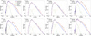 |
Fig. 1 SEDs and best-fit DUSTY models for the dusty AGB stars. Solid blue line: input spectra; solid red line: total DUSTY model; dotted cyan line: attenuated input spectral component; dashed green line: dust scattered component; dot-dashed orange line: dust thermal component. Photometric fluxes are indicated as filled circles (in a few cases the variability-induced uncertainties are larger than the average value), photometric data not included in the analysis as empty circles, and upper limits as empty triangles. Solid grey lines are GAIA, IRAS, and ISO spectra; shadowed areas indicate 10% uncertainties. |
Best-fit parameters from DUSTY models.
Properties of stars for which DUSTY models show no dust component.
4.2 Derivation of related parameters
We derived the bolometric luminosity, the inner and outer radii of the CSE (Rinn, Rout), the radial optical depth as a function of wavelength (see also Appendix C), and the dust mass (Mdust) from the spatial integration of the density distribution (see Eq. (1) of Sahai et al. 2023):
 (5)
(5)
where y(Y)=(Y3-n−1)/(1-Y1-n), and τλ and κλ are, respectively, the radial optical depth of the shell and the dust mass absorption coefficient at a certain wavelength. In the case of a dust grain mixture, DUSTY considers only one type of grain whose properties are averaged from those of the mixture according to their abundances (see Ivezic & Elitzur 1995, 1997).
We considered 60 μm as the reference wavelength, which is long enough with respect to the assumed grain sizes that grain size does not affect significantly the dust mass absorption coefficient (see e.g. Ysard et al. 2018). The mass absorption coefficients were estimated from their respective complex refractive indexes applying the Mie theory (see e.g. Draine & Lee 1984; Ivezic & Elitzur 1997 and references therein).
We obtained the values of κ60 μm for each dust composition used in this study. The different mixtures of O-rich dust has κ60 μm≃100 cm2 g−1 (with small differences between them) and the mixture of C-rich dust has κ60 μm≃90 cm2 g−1. These κ60 μm estimates are in good agreement with common values from the literature (e.g. Fig. 3 from Ysard et al. 2018).
In the case of VY UMa, we estimated the dust shell masses for the two different components: the present-day CSE (pointsource) and the detached shell (extended). This separation allows a more direct comparison with the rest of the sample. The present-day CSE has the lowest dust shell mass among the dusty sources (1.5×10⁻⁷ M⊙), indicating that the mass-loss process was resumed recently.
The sample presents a wide range of masses, ranging from 1.5×10⁻⁷ to 1.2×10⁻³ M⊙. These mass estimates have a strong dependence on Y (Mdust∝Y3-n; i.e. linearly when n=2), which is a relatively uncertain parameter.
 |
Fig. 3 Histograms showing the distributions of the best-fit solution SED modelling parameters. From left to right: stellar effective temperature, dust inner radius temperature, density power-law index, dust shell radial optical depth at 550 nm. White bins represent ‘naked’ O-rich uvAGBs, grey bins represent O-rich uvAGBs with dust component, and striped bins represent C-rich uvAGBs. |
4.3 Dust mass-loss rates and gas-to-dust ratio
We performed a comparison between the dust properties obtained in this study and those from the molecular gas component estimated by Alonso-Hernández et al. (2024). For this, we assumed that the expansion velocity of the dust (Vdust) is similar to that of CO and estimated the dust mass-loss rates by dividing the dust masses over the dust expansion times (texp=Rout/Vdust):
 (6)
(6)
Even though the dust masses estimated have a large dependence on Y, which is uncertain in some cases, the derived dust mass-loss rates are much less dependent on Y because the expansion time compensates for this dependence (exactly when n=2) and our estimated values of n are close to two. We therefore estimated the average gas-to-dust ratios as the ratio between the gas and dust mass-loss rates:
 (7)
(7)
where we used the Ṁgas estimates from Alonso-Hernández et al. (2024). Although the dust expansion velocities are expected to be somewhat greater than those of the gas because of the finite drift velocity of the dust grains relative to the gas, this difference is not significant for the dust mass-loss rate estimates and produces only slight differences (see Groenewegen et al. 1998).
We obtained moderate dust mass-loss rates, in the 0.05-65×10−10 M⊙ yr−1 range. The lowest estimate corresponds to the present-day CSE of VY UMa (5×10⁻¹² M⊙ yr−1), in which the estimation of δ is not straightforward due to the presence of two components in the dust, whereas only one was detected in CO. Therefore, we assumed that the CO emission and gas mass-loss rate are related to the present-day dust CSE, and we used it to estimate δ, which has a high value of 40 000. The rest of the δ values in the sample cover the ~50-1700 range.
4.4 Trends and comparison with larger samples
In this work, we characterised the dust component in CSEs of uvAGBs and estimated the gas-to-dust ratio by comparing the gas and dust mass-loss rates. The next step was to assess whether these parameters are sensitive to the UV emission and its underlying mechanism or are determined by the stellar properties.
For this purpose, we performed a comparison with one independent stellar property and one extrinsic to the star. For the intrinsic stellar property, we used the variability classification and pulsation period (P) from Samus’ et al. (2017), summarised for this sample in Alonso-Hernández et al. (2024). For the extrinsic parameter, we used RFUV/NUV, which is associated with binarity (when ≳0.06, see Sahai et al. 2022) and large UV excesses (see Appendix C).
Fig. 4 shows the HRD for our sample, in which the dust shell masses and variability classification are also shown. We found that ‘naked’ stars are located in the bottom left corner (low luminosity and high temperature), which is consistent with an early evolutionary stage and indicates that they are not undergoing a significant mass-loss process yet. On the other hand, AGB stars with larger dust masses are located in the top right corner (high luminosity and low temperature); these sources are in a more evolved stage and have more mass accumulated in their CSE. An evolutionary trend can also be seen over the AGB, where irregular pulsators are located in the bottom left corner, Miras pulsators are mostly located in the top right, and Semi-regulars are spread over the other two groups.
Fig. 5 shows the comparisons between the most relevant parameters estimated from the SED modelling with P and  (defined as Rfuv/nuv corrected from dust attenuation, see Appendix C). We evaluated these comparisons qualitatively because the strong dependence of these parameters and different methodologies employed in the literature prevented us from deriving simple relationships for comparison (see discussion in Sect. 2 of Höfner & Olofsson 2018)
We found a decreasing (non-linear) trend of T* with P (see Fig. 5 top left). This relationship is a trend through the AGB, in which the stellar effective temperatures decrease while pulsation periods increase as the stars climb the AGB.
No clear correlation was found between Tinn and P (see Fig. 5 middle, top left), indicating that Tinn does not depend directly on the pulsations and related stellar parameters. Low Tinn values indicate a lack of warm dust, which might result from a recent decrease in the mass-loss rate or from the accumulation of dust in structures at a certain distance from the star.
We also noted a dichotomy in the values of n (see Fig. 5 middle, bottom left). Miras present standard values with n~2.0 on average, whereas semi-regulars systematically present lower values, with n~1.8 on average. Even though this result does not have a direct interpretation, the systematically lower values can be related to deviations from homogeneous outflows, in which pulsation-driven mass-loss would contribute more significantly in semi-regulars than in Miras.
We also found a positive (non-linear) correlation between τ550 and P (see Fig. 5 bottom left). The optical depth is proportional to the mass-loss rate, which increases with P (see e.g. McDonald & Zijlstra 2016), and indicates that the dust production rates are higher for more evolved stars.
On the other hand, no clear correlations were found between the parameters estimated from the SED modelling and  (see Fig. 5 right panels). Only a slight decreasing trend of the stellar temperature with
  might be seen. This correlation, although weak, is expected due (in part) to the contribution of the stellar photospheric emission in the NUV band increasing with T*, whereas its effect in the FUV band is negligible as it is dominated by accretion or chromospheric emission. Therefore, stars with larger Ti present systematically lower RFUV/NUV.
Fig. 6 shows the comparison between the gas and dust massloss rate estimates for our sample of uvAGBs and those estimated by Wallström et al. (2025) for the Nearby Evolved Stars Survey (NESS, Scicluna et al. 2022) sample, which includes 485 AGB stars. Our CO-detected uvAGBs are located at moderate gas and dust mass-loss rates (6×10⁻⁸ M⊙ yr−1 ≲ Mgas ≲ 3×10⁻⁶ M⊙ yr−1 and 5×10⁻¹²M⊙ yr−1 ≲ Mdust ≲ 7×10⁻⁹ M⊙ yr−1) and, apart from VY UMa, show a good agreement with values derived from the NESS sample.
We found that our sources are in good agreement with those of NESS and are spread around the trend shown in Wallström et al. (2025). Furthermore, we note that the two C-rich AGB stars and the four O-rich Miras in our sample are systematically found to be above this trend. We expand the comparison with the NESS sample in Appendix F.
Finally, we searched for correlations between the gas-to-dust ratio (δ) and different parameters (see Fig. 7). We used the linear correlation coefficient (r) as a simple statistical indicator to identify first-order trends (we refer to |r|>0.7 and 0.7<|r|<0.3 as strong and weak correlations, respectively).
We checked the positive correlation between δ and the ratio between CO intensity and IRAS 60 μm flux (r=0.37). When rejecting R UMa, which has a significant dispersion in the FIR photometry (see Sect. 3.2), this correlation becomes stronger (r=0.63). We also found weak positive correlations of δ with Ṁgas (r=0.51) and P (r=0.64), whereas a weak anti-correlation was found with  (r=−0.44).
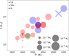 |
Fig. 4 HRD of our the sample. The size of the markers is proportional to the dust shell masses as shown in the bottom right legend. The marker’s colour represents the variability type. Red: semi-regulars (SRs), green: irregulars (LB), and blue: Miras (M). The shape of the markers represents the chemistry of the AGB stars. Circles: O-rich (‘naked’ as asterisks), crosses: C-rich. |
5 Discussion
In this study, we characterised the dusty envelopes in a sample of 29 UV emitting AGB stars, which are binary candidates. In particular, we searched for trends between the parameters obtained from SED modelling, the pulsation properties, and the UV emission. We also performed a comparison with the NESS sample of AGB stars to discern whether uvAGBs present systematic differences in their mass-loss rates or gas-to-dust ratios.
We found that UV emitting AGB stars cannot be clearly differentiated from the rest of the AGB stars, on the basis of their SED shapes, mass-loss rates or gas-to-dust ratios. This result is rather surprising considering the variety of binary-related physical phenomena that may affect the mass loss, dust formation and enrichment, and gas-to-dust ratios in uvAGBs. In particular, we list the following results below:
In uvAGBs, the internal UV/X-ray emission may photodissociate the abundance of CO in the innermost regions on the envelope. These abundance depletions can subtly modify the CO line profiles and intensities, remaining unperceived and affecting the gas mass-loss rate estimates (e.g. a factor ~2 for T Dra, see Alonso-Hernández et al. 2025).
Considering that uvAGBs are likely binary systems, they can suffer alterations in the dust formation process, especially in the wake of orbiting close stellar companions, where dust has been proposed to form abundantly (Danilovich et al. 2025). Similarly, the impact of UV emission on the abundances of dust precursor molecular species (e.g. SiO and C2H2, see Van de Sande & Millar 2019, 2022) may affect dust formation.
The presence of binary-induced structures (e.g. spirals and discs), which usually cannot be directly identified by CO line profiles or SED modelling, may lead to incorrect estimates of the mass-loss rates for both dust (see Wiegert et al. 2020) and gas (see Vermeulen et al. 2025) when assuming spherical geometry.
The combination of these phenomena can potentially produce variations in the mass-loss rates by orders of magnitude. Even though it might be expected that uvAGBs have lower gas-to-dust ratios as suggested by Alonso-Hernández et al. (2024), these phenomena may compensate each other in the overall result. On the other hand, some properties of dust grains (e.g. composition, size) in these systems may differ due to the UV irradiation or effects of stellar companions on the environment.
We also remark that binarity is expected to be common in AGB stars. In particular, the fraction of uvAGBs is at least 10% of the total population (see Alonso-Hernández et al. 2024). Therefore, it is likely that the uvAGBs present in the NESS sample (see Appendix C) were producing an overlap when we compared the samples, preventing a clear identification of differences.
We also show that modelling dust attenuation at UV wavelengths is necessary for extracting intrinsic UV emission properties (see Appendix C). Optically thick CSEs can prevent even the detection of sources with intrinsically intense UV emission, resulting in an underestimation of the percentages of uvAGBs (as suggested by Montez et al. 2017).
We also highlight the effect of dust attenuation on the RFUV/NUV≳0.06 threshold proposed by Sahai et al. (2022) as a criterion to discern cases in which the UV excesses are clearly related with accretion processes. The observed RFUV/NUV may well differ from the intrinsic ratio due to the difference in the optical depths between both bands. The optical depth in the FUV band is larger than in the NUV band, leading to intrinsic RFUV/NUV larger than observed. O-rich AGB stars present a larger difference in the optical depth between both bands (see Appendix C).
The wavelength dependence of dust attenuation also affects the overall shape of the UV spectra, affecting both continuum measurements and line-intensity ratios. Although this effect is small when comparing spectral lines and their adjoining continuum emission (e.g. Guerrero & Ortiz 2020), it can be important when measuring the continuum over a broad spectral range or when estimating ratios between distant spectral lines due to the difference in attenuation (e.g. Ortiz et al. 2019).
We found a weak anticorrelation between the gas-to-dust ratio and  , although we acknowledge that the uncertainties associated with the dust attenuation correction and the intrinsic variability of the UV emission in these sources may well be hiding a stronger anticorrelation with
  . Furthermore, the correlations between the gas-to-dust ratio with the mass-loss rate and stellar pulsations are stronger (see Fig. 7).
In this context, we remark that uvAGBs are predominantly semi-regulars (see Alonso-Hernández et al. 2024) and have moderate or low mass-loss rates (the dust attenuation produces an observational bias to detect UV emission in AGB stars with low opacities), which have systematically lower gas-to-dust ratios. Future studies are required to better understand the effect of UV emission on gas-to-dust ratios.
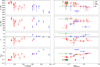 |
Fig. 5 Comparison of the best-fit solution SED modelling parameters (from top to bottom : T*, Tinn, n and τ550) with P (left) and |


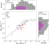 |
Fig. 6 Comparison between the gas and dust mass-loss rates for our sample of uvAGBs. The colour and shape of the markers represent the stellar variability and chemistry type as in Fig. 4. Grey markers represent sources from the NESS sample. The dashed line represents the relationship presented in Wallström et al. (2025). The histograms at the top and to the right of the figure indicate the distribution of Ṁdust and Ṁgas respectively. |
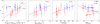 |
Fig. 7 Comparison between the gas-to-dust ratio and different parameters (from left to right : ratio of CO J=2-1 velocity-integrated line flux to the IRAS 60 μm flux, Ṁgas, P, and |


6 Summary and conclusions
In this work, we studied the dust properties of UV emitting AGB stars estimated from SED modelling. We included the reduction of Herschel/PACS images and performed aperture photometry, which was useful to check the angular sizes and density distributions of the CSEs and to model the extended detached shell of the C-rich AGB star VY UMa.
We obtained moderate dust mass-loss rates in the range 10−10−10−8 M⊙ yr−1 and gas-to-dust ratios ranging from 50 to 1700 (excluding VYUMa, see Table 1), which are intermediate values in comparison with those estimated for the NESS sample (see Fig. 4.3 and Appendix F). Our sample of uvAGBs presents similar mass-loss rates and shows, at least qualitatively, the same trends as larger samples of AGB stars. However, it is expected that larger samples also contain some uvAGBs as they are at least 10% of the population(see Alonso-Hernández et al. 2024), which may prevent us from identifying clear differences.
We found a weak anticorrelation (r=−0.44) between the gas-to-dust ratio and  . This result indicates that the gas-to-dust ratio of uvAGBs with larger
  might be more affected by UV emission and/or by the presence of a stellar companions. However, we note that
  is affected by the uncertainties on the dust attenuation correction as well as the intrinsic UV variability found in uvAGBs. On the other hand, the gas-to-dust ratio is also affected by pulsations and mass-loss rates. Therefore, the relationship between the gas-to-dust ratio and the UV emission is not simple.
It is important to obtain not only samples with confirmed stellar companions, but also of single (or not interacting) stellar systems, to better understand the effect of binarity on mass-loss processes. Future observations with high angular resolution are required to explore the dust-forming regions surrounding these stars, identify the presence of stellar companions, and constrain their effect on dust formation and enrichment.
Infrared interferometry is useful to observe the dust distribution in the stellar vicinity, which is key to identifying whether dust formation can be correctly described by radiatively driven winds (Răstău et al. 2026), or to indicate the presence of stellar companions (see e.g. Planquart et al. 2024). Sub-millimetre interferometry has already shown significant capabilities to identify binary-induced structure and modified dynamic in the interior of CSEs (see e.g. Decin et al. 2020). Moreover, larger spectral coverage is required for robust SED modelling, especially extending into the far-infrared, which traces the outermost regions of the CSEs where a significant mass of cool dust may reside.
We also described the effects of dust attenuation on the observed UV emission and the importance of correct modelling when analysing photometric or spectroscopic observations. Correct modelling of dust attenuation can provide a better understanding of the nature of the UV source (e.g. UV excesses and Rfuv/nuv) as it is not negligible in some cases. Furthermore, dust attenuation can prevent the detection of uvAGBs.
The detectability of UV emission is biased towards AGB stars with low mass-loss rates (and low opacities), which have systematically lower gas-to-dust ratios. A systematic study, using a larger sample, in which binary and single AGB stars are identified, and covering wider ranges of parameters, would help to refine the observed trends with the mass-loss properties.
Data availability
Tables containing the employed photometry for the SEDs and the photometric fluxes estimated from the individual Herschel/PACS observations are available at the CDS via https://cdsarc.cds.unistra.fr/viz-bin/cat/J/A+A/709/A143
Acknowledgements
We thank the referee, Roberto Ortiz, whose valuable comments helped us improve the quality of the manuscript. This work is part of the I+D+i projects PID2019-105203GB-C22, PID2022-137241NB-C42 and PID2023-146056NB-C22 funded by Spanish MCIN/AEI/10.13039/501100011033 and by “ERDF A way of making Europe″. J.A.H. is supported by INTA grant PRE_MDM_05 and acknowledges CSIC grant iMOVE 23023. R.S.’s contribution to the research described here was carried out at the Jet Propulsion Laboratory, California Institute of Technology, under a contract with NASA (80NM0018D0004), and funded in part by NASA via various ROSES/ADAP awards and HST/GO awards (administered by STScI). Herschel is an ESA space observatory with science instruments provided by European-led Principal Investigator consortia and with important participation from NASA. ISO is an ESA project with instruments funded by ESA Member States and with the participation of ISAS and NASA. Some of the data presented in this paper were obtained from the Multimission Archive at the Space Telescope Science Institute (MAST). STScI is operated by the Association of Universities for Research in Astronomy, Inc., under NASA contract NAS5-26555. Support for MAST for non-HST data is provided by the NASA Office of Space Science via grant NAG5-7584 and by other grants and contracts.
References
- Agúndez, M., Martínez, J. I., de Andres, P. L., Cernicharo, J., & Martín-Gago, J. A. 2020, A&A, 637, A59 [Google Scholar]
- Alonso-Hernández, J., Sánchez Contreras, C., & Sahai, R. 2024, A&A, 684, A77 [NASA ADS] [CrossRef] [EDP Sciences] [Google Scholar]
- Alonso-Hernández, J., Sánchez Contreras, C., Agúndez, M., et al. 2025, A&A, 698, A319 [NASA ADS] [CrossRef] [EDP Sciences] [Google Scholar]
- Aringer, B., Girardi, L., Nowotny, W., Marigo, P., & Bressan, A. 2016, MNRAS, 457, 3611 [Google Scholar]
- Aringer, B., Marigo, P., Nowotny, W., et al. 2019, MNRAS, 487, 2133 [CrossRef] [Google Scholar]
- Balick, B., & Frank, A. 2002, ARA&A, 40, 439 [Google Scholar]
- Begemann, B., Dorschner, J., Henning, T., et al. 1997, ApJ, 476, 199 [NASA ADS] [CrossRef] [Google Scholar]
- Castro-Carrizo, A., Quintana-Lacaci, G., Neri, R., et al. 2010, A&A, 523, A59 [NASA ADS] [CrossRef] [EDP Sciences] [Google Scholar]
- Clegg, P. E., Ade, P. A. R., Armand, C., et al. 1996, A&A, 315, L38 [NASA ADS] [Google Scholar]
- Cox, N. L. J., Kerschbaum, F., van Marle, A. J., et al. 2012, A&A, 537, A35 [NASA ADS] [CrossRef] [EDP Sciences] [Google Scholar]
- Danilovich, T., Samaratunge, N., Mori, Y. L., et al. 2025, A&A, 704, A341 [NASA ADS] [CrossRef] [EDP Sciences] [Google Scholar]
- De Angeli, F., Weiler, M., Montegriffo, P., et al. 2023, A&A, 674, A2 [NASA ADS] [CrossRef] [EDP Sciences] [Google Scholar]
- de Graauw, T., Haser, L. N., Beintema, D. A., et al. 1996, A&A, 315, L49 [NASA ADS] [Google Scholar]
- De Marco, O. 2009, PASP, 121, 316 [NASA ADS] [CrossRef] [Google Scholar]
- Decin, L., Montargès, M., Richards, A. M. S., et al. 2020, Science, 369, 1497 [Google Scholar]
- Dehaes, S., Groenewegen, M. A. T., Decin, L., et al. 2007, MNRAS, 377, 931 [NASA ADS] [CrossRef] [Google Scholar]
- Doi, Y., Takita, S., Ootsubo, T., et al. 2015, PASJ, 67, 50 [NASA ADS] [Google Scholar]
- Draine, B. T., & Lee, H. M. 1984, ApJ, 285, 89 [NASA ADS] [CrossRef] [Google Scholar]
- Duquennoy, A., & Mayor, M. 1991, A&A, 248, 485 [NASA ADS] [Google Scholar]
- Ferrarotti, A. S., & Gail, H. P. 2006, A&A, 447, 553 [CrossRef] [EDP Sciences] [Google Scholar]
- Gordon, K. D., Clayton, G. C., Decleir, M., et al. 2023, ApJ, 950, 86 [CrossRef] [Google Scholar]
- Graciá-Carpio, J., Wetzstein, M., & Roussel, H. 2015, arXiv e-prints [arXiv:1512.03252] [Google Scholar]
- Groenewegen, M. A. T. 2022, A&A, 659, A145 [NASA ADS] [CrossRef] [EDP Sciences] [Google Scholar]
- Groenewegen, M. A. T., Whitelock, P. A., Smith, C. H., & Kerschbaum, F. 1998, MNRAS, 293, 18 [NASA ADS] [CrossRef] [Google Scholar]
- Gry, C., Swinyard, B., Harwood, A., et al. 2003, The ISO Handbook, Volume III - LWS - The Long Wavelength Spectrometer [Google Scholar]
- Guerrero, M. A., & Ortiz, R. 2020, MNRAS, 491, 680 [NASA ADS] [CrossRef] [Google Scholar]
- Hanner, M. 1988, Grain optical properties, in NASA, Washington, Infrared Observations of Comets Halley and Wilson and Properties of the Grains, 22 (SEE N89-13330 04-89) [Google Scholar]
- Henning, T., Begemann, B., Mutschke, H., & Dorschner, J. 1995, A&AS, 112, 143 [Google Scholar]
- Heras, A. M., & Hony, S. 2005, A&A, 439, 171 [NASA ADS] [CrossRef] [EDP Sciences] [Google Scholar]
- Höfner, S., & Olofsson, H. 2018, A&A Rev., 26, 1 [Google Scholar]
- Ivezic, Z., & Elitzur, M. 1995, ApJ, 445, 415 [NASA ADS] [CrossRef] [Google Scholar]
- Ivezic, Z., & Elitzur, M. 1997, MNRAS, 287, 799 [Google Scholar]
- Ivezic, Z., Nenkova, M., & Elitzur, M. 1999, Astrophysics Source Code Library [record ascl:9911.001] [Google Scholar]
- Jenness, T., Stevens, J. A., Archibald, E. N., et al. 2002, MNRAS, 336, 14 [NASA ADS] [CrossRef] [Google Scholar]
- Jones, O. C., Kemper, F., Srinivasan, S., et al. 2014, MNRAS, 440, 631 [NASA ADS] [CrossRef] [Google Scholar]
- Kemper, F., de Koter, A., Waters, L. B. F. M., Bouwman, J., & Tielens, A. G. G. M. 2002, A&A, 384, 585 [NASA ADS] [CrossRef] [EDP Sciences] [Google Scholar]
- Kessler, M. F., Steinz, J. A., Anderegg, M. E., et al. 1996, A&A, 315, L27 [NASA ADS] [Google Scholar]
- Kessler, M. F., Mueller, T. G., Leech, K., et al. 2003, The ISO Handbook, Volume I - Mission & Satellite Overview (European Space Agency) [Google Scholar]
- Kwitter, K. B., & Henry, R. B. C. 2022, PASP, 134, 022001 [NASA ADS] [CrossRef] [Google Scholar]
- Leech, K., Kester, D., Shipman, R., et al. 2003, The ISO Handbook, Volume V - SWS - The Short Wavelength Spectrometer (European Space Agency) [Google Scholar]
- Martin, D. C., Fanson, J., Schiminovich, D., et al. 2005, ApJ, 619, L1 [Google Scholar]
- Mathis, J. S., Rumpl, W., & Nordsieck, K. H. 1977, ApJ, 217, 425 [Google Scholar]
- McDonald, I., & Zijlstra, A. A. 2016, ApJ, 823, L38 [NASA ADS] [CrossRef] [Google Scholar]
- Mečina, M., Kerschbaum, F., Groenewegen, M. A. T., et al. 2014, A&A, 566, A69 [NASA ADS] [CrossRef] [EDP Sciences] [Google Scholar]
- Mečina, M., Aringer, B., Nowotny, W., et al. 2020, A&A, 644, A66 [NASA ADS] [CrossRef] [EDP Sciences] [Google Scholar]
- Miszalski, B., Acker, A., Moffat, A. F. J., Parker, Q. A., & Udalski, A. 2009, A&A, 496, 813 [NASA ADS] [CrossRef] [EDP Sciences] [Google Scholar]
- Montez, Rodolfo, J., Ramstedt, S., Kastner, J. H., Vlemmings, W., & Sanchez, E. 2017, ApJ, 841, 33 [NASA ADS] [CrossRef] [Google Scholar]
- Neugebauer, G., Habing, H. J., van Duinen, R., et al. 1984, ApJ, 278, L1 [NASA ADS] [CrossRef] [Google Scholar]
- Nordhaus, J., & Blackman, E. G. 2006, MNRAS, 370, 2004 [NASA ADS] [CrossRef] [Google Scholar]
- Ochsenbein, F., Bauer, P., & Marcout, J. 2000, A&AS, 143, 23 [Google Scholar]
- Onaka, T., de Jong, T., Yamamura, I., Cami, J., & Tanab’e, T. 1999, in ESA Special Publication, 427, The Universe as Seen by ISO, eds. P. Cox, & M. Kessler, 381 [Google Scholar]
- Ortiz, R., & Guerrero, M. A. 2016, MNRAS, 461, 3036 [NASA ADS] [CrossRef] [Google Scholar]
- Ortiz, R., & Guerrero, M. A. 2021, ApJ, 912, 93 [Google Scholar]
- Ortiz, R., Guerrero, M. A., & Costa, R. D. D. 2019, MNRAS, 482, 4697 [CrossRef] [Google Scholar]
- Ott, S. 2010, in Astronomical Society of the Pacific Conference Series, 434, Astronomical Data Analysis Software and Systems XIX, eds. Y. Mizumoto, K. I. Morita, & M. Ohishi, 139 [Google Scholar]
- Pegourie, B. 1988, A&A, 194, 335 [NASA ADS] [Google Scholar]
- Piazzo, L., Calzoletti, L., Faustini, F., et al. 2015, MNRAS, 447, 1471 [NASA ADS] [CrossRef] [Google Scholar]
- Pilbratt, G. L., Riedinger, J. R., Passvogel, T., et al. 2010, A&A, 518, L1 [NASA ADS] [CrossRef] [EDP Sciences] [Google Scholar]
- Planquart, L., Paladini, C., Jorissen, A., et al. 2024, A&A, 687, A306 [NASA ADS] [CrossRef] [EDP Sciences] [Google Scholar]
- Poglitsch, A., Waelkens, C., Geis, N., et al. 2010, A&A, 518, L2 [NASA ADS] [CrossRef] [EDP Sciences] [Google Scholar]
- Ramstedt, S., Montez, R., Kastner, J., & Vlemmings, W. H. T. 2012, A&A, 543, A147 [NASA ADS] [CrossRef] [EDP Sciences] [Google Scholar]
- Rastau, V., Paladini, C., Drevon, J., et al. 2026, A&A, 705, A127 [Google Scholar]
- Rodrigo, C., & Solano, E. 2020, in XIV.0 Scientific Meeting (virtual) of the Spanish Astronomical Society, 182 [Google Scholar]
- Rodrigo, C., Solano, E., & Bayo, A. 2012, SVO Filter Profile Service Version 1.0, IVOA Working Draft 15 October 2012 [Google Scholar]
- Rodrigo, C., Cruz, P., Aguilar, J. F., et al. 2024, A&A, 689, A93 [NASA ADS] [CrossRef] [EDP Sciences] [Google Scholar]
- Sahai, R., & Trauger, J. T. 1998, AJ, 116, 1357 [NASA ADS] [CrossRef] [Google Scholar]
- Sahai, R., Morris, M., Sánchez Contreras, C., & Claussen, M. 2007, AJ, 134, 2200 [NASA ADS] [CrossRef] [Google Scholar]
- Sahai, R., Findeisen, K., Gil de Paz, A., & Sánchez Contreras, C. 2008, ApJ, 689, 1274 [NASA ADS] [CrossRef] [Google Scholar]
- Sahai, R., Morris, M. R., & Villar, G. G. 2011a, AJ, 141, 134 [NASA ADS] [CrossRef] [Google Scholar]
- Sahai, R., Neill, J. D., Gil de Paz, A., & Sánchez Contreras, C. 2011b, ApJ, 740, L39 [NASA ADS] [CrossRef] [Google Scholar]
- Sahai, R., Sanz-Forcada, J., Sánchez Contreras, C., & Stute, M. 2015, ApJ, 810, 77 [NASA ADS] [CrossRef] [Google Scholar]
- Sahai, R., Sanz-Forcada, J., & Sánchez Contreras, C. 2016, in Journal of Physics Conference Series, 728, 042003 [Google Scholar]
- Sahai, R., Sánchez Contreras, C., Mangan, A. S., et al. 2018, ApJ, 860, 105 [NASA ADS] [CrossRef] [Google Scholar]
- Sahai, R., Sanz-Forcada, J., Guerrero, M., Ortiz, R., & Contreras, C. S. 2022, Galaxies, 10, 62 [NASA ADS] [CrossRef] [Google Scholar]
- Sahai, R., Bujarrabal, V., Quintana-Lacaci, G., et al. 2023, ApJ, 943, 110 [NASA ADS] [CrossRef] [Google Scholar]
- Samus’, N. N., Kazarovets, E. V., Durlevich, O. V., Kireeva, N. N., & Pastukhova, E. N. 2017, Astron. Rep., 61, 80 [Google Scholar]
- Scicluna, P., Kemper, F., McDonald, I., et al. 2022, MNRAS, 512, 1091 [NASA ADS] [CrossRef] [Google Scholar]
- Sloan, G. C., & Price, S. D. 1995, ApJ, 451, 758 [Google Scholar]
- Sloan, G. C., Kraemer, K. E., Goebel, J. H., & Price, S. D. 2003a, ApJ, 594, 483 [Google Scholar]
- Sloan, G. C., Kraemer, K. E., Price, S. D., & Shipman, R. F. 2003b, ApJS, 147, 379 [CrossRef] [Google Scholar]
- Sloan, G. C., Kraemer, K. E., & Volk, K. 2025, ApJS, 279, 15 [Google Scholar]
- Speck, A. K., Barlow, M. J., Sylvester, R. J., & Hofmeister, A. M. 2000, A&AS, 146, 437 [Google Scholar]
- Stanghellini, L., Shaw, R. A., & Villaver, E. 2016, ApJ, 830, 33 [NASA ADS] [CrossRef] [Google Scholar]
- Suh, K.-W. 2018, J. Korean Astron. Soc., 51, 155 [Google Scholar]
- Tachibana, K., Miyata, T., Kamizuka, T., et al. 2023, PASJ, 75, 489 [Google Scholar]
- Tielens, A. G. G. M. 2005, The Physics and Chemistry of the Interstellar Medium (Cambridge University Press) [Google Scholar]
- Ueta, T., Meixner, M., & Bobrowsky, M. 2000, ApJ, 528, 861 [Google Scholar]
- Van de Sande, M., & Millar, T. J. 2019, ApJ, 873, 36 [CrossRef] [Google Scholar]
- Van de Sande, M., & Millar, T. J. 2022, MNRAS, 510, 1204 [Google Scholar]
- van Marle, A. J., Cox, N. L. J., & Decin, L. 2014, A&A, 570, A131 [NASA ADS] [CrossRef] [EDP Sciences] [Google Scholar]
- Vermeulen, O., Esseldeurs, M., Malfait, J., et al. 2025, A&A, 700, A85 [NASA ADS] [CrossRef] [EDP Sciences] [Google Scholar]
- Wallström, S. H. J., Scicluna, P., Srinivasan, S., et al. 2025, A&A, 704, A276 [NASA ADS] [CrossRef] [EDP Sciences] [Google Scholar]
- Waters, L. B. F. M. 2011, in Astronomical Society of the Pacific Conference Series, 445, Why Galaxies Care about AGB Stars II: Shining Examples and Common Inhabitants, eds. F. Kerschbaum, T. Lebzelter, & R. F. Wing, 227 [Google Scholar]
- Wiegert, J., Groenewegen, M. A. T., Jorissen, A., Decin, L., & Danilovich, T. 2020, A&A, 642, A142 [NASA ADS] [CrossRef] [EDP Sciences] [Google Scholar]
- Ysard, N., Jones, A. P., Demyk, K., Boutéraon, T., & Koehler, M. 2018, A&A, 617, A124 [NASA ADS] [CrossRef] [EDP Sciences] [Google Scholar]
Publicly available on https://users.physics.unc.edu/~gcsloan/library/lrsatlas
Publicly available on https://users.physics.unc.edu/~gcsloan/library/swsatlas
Publicly available on http://stev.oapd.inaf.it/atm/index.html
Appendix A Semi-extended sources
Fig. A.1 shows radial surface brightness profiles for the four semi-extended sources presented in this study (RU Her, SV Peg, TDra and VEri). In addition, we created DUSTY synthetic images for their best-fit models in the effective wavelength of each Herschel/PACS filter and convolved them with their respective PSFs. Then, we radially averaged the surface brightness, in both the observed and the synthetic images, in radial annuli of 1″ and compared them. The uncertainties were estimated as the sum of the standard deviation of the flux and the average instrumental error in each annulus.
The best-fit DUSTY models (see Sect. 4.1) reproduce correctly the angular sizes after convolving with the correspondent PSF. In the four cases the difference between the angular sizes and the Herschel/PACS PSFs can be appreciated better on the B filter (70 μm) due to its higher angular resolution.
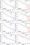 |
Fig. A.1 Radial surface brightness profiles at 70 μm (left) and 160 μm (right) for the four semi-extended sources in the sample (from top to bottom : RU Her, SV Peg, TDra and VEri). Solid circles correspond to Herschel/PACS radial surface brightness profiles, dashed lines to DUSTY synthetic images convolved with their respective PSFs and dotted lines to the PSFs to represent point-source radial surface brightness. |
Appendix B VYUMa detached shell
We present a more detailed analysis of the SED modelling for the particular case of VY UMa, which has a large-scale detached shell in addition to a compact, bright central emission component that represents the present-day mass-loss rate. This extended emission was previously identified in the Herschel/PACS images (Cox et al. 2012; van Marle et al. 2014) and manifested in the SED as the large excesses in the far-infrared (see the case of VY UMa in Fig. D.1).
The contribution of the detached shell is only noticed in the SED in the far-infrared because it is composed of very cold dust (~10-100K), whose emission is concentrated in the ~30-300 μm region, and it does not modify the SED at shorter wavelengths. Therefore, we used the Herschel/PACS fluxes, which isolates the present-day mass-loss (black filled circles in Fig. D.1) and the extended emission from the detached shell (black filled diamonds in Fig. D.1), and rejected IRAS and AKARI because they included partially the emission form the detached shell.
To correctly fit the SED, we followed a similar methodology to that presented in Mečina et al. (2014, 2020) to separate the contribution from the present-day mass-loss and the detached shell. We started by fitting the SED of the present-day mass-loss (including Herschel/PACS fluxes and all the photometric observations at λ<30 μm) following the same procedure as in the rest of the sources. Once the best-fit solution for the present-day mass-loss was found, we modified the normalised density distribution including a peak at 3200-8000×Rinn, which is equivalent to 31-78″ considering the source distance and in agreement with the location of the detached shell (see Fig. B.1).
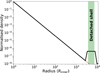 |
Fig. B.1 Adopted density profile for VY UMa. The solid black line represents the modified density distribution to fit the detached shell. The dotted red line represents the smooth density profile from the presentday mass-loss. The green area represent the location of the detached shell in the Herschel/PACS images. |
This model reproduces satisfactorily both the FIR excesses and the Herschel/PACS radial surface brightness profiles. It allows us to estimate an overall density and dust mass of the extended detached shell. However, we note that this single 1D model is not able to reproduce the asymmetrical shape of the detached shell, which would require a more advanced 3D radiative transfer model.
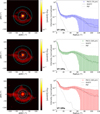 |
Fig. B.2 Left : Herschel/PACS images of VYUMa. The solid cyan represents the aperture used to isolate the central component (representing the present-day mass-loss), and the dashed cyan lines the aperture used to measure the extended detached shell. Right : Radial surface brightness profiles, the markers indicate the surface brightness from the images, the dashed line the surface brightness from DUSTY models convolved with their respective Herschel/PACS PSFs, and the dotted lines the Herschel/PACS PSFs. |
Appendix C UV excesses and dust attenuation
We computed synthetic stellar photometry on the GALEX bands and compared them with the observed fluxes to estimate the UV excesses (similarly to Sahai et al. 2008; Ortiz & Guerrero 2016). We noted that GALEX NUV and FUV photometric bands fall outside the wavelength range covered by the COMARCS models used in this work (see Sect. 3). Therefore, the stellar fluxes were estimated by extrapolating the input spectra following a blackbody distribution and convolving it with the transmission curves of their respective filters. Table C.1 shows the observed and modelled properties of the UV emission for the sources used in this sample.
We acknowledge that the real stellar spectrum differs from a blackbody approximation mainly due to the presence of (i) molecular absorption bands, and (ii) emission-line features due to possible chromospheric emission, that can produce a significant effect on the shape of the stellar spectra in the UV. The features in (ii) are expected to have a much stronger effect in the FUV (compared to the NUV) where the photospheric contribution is relatively much weaker. Note that the sole purpose of this simple approximation is to explore whether RFUV/NUV is a reasonable proxy for the FUV excess.
UV emission parameters derived from GALEX observations and SED modelling.
In addition, the UV spectral range is specially affected by circumstellar dust attenuation, which might imply a large difference between the intrinsic and the observed UV emission, therefore, affecting the estimation of the UV excesses. Moreover, the wavelength dependency of the opacity produces a variation of the RFUV/NUV.
Fig. C.1 shows the opacity curves for the generic dust composition of C-rich AGB stars and O-rich AGB stars described in Sect. 3.1 provided by DUSTY as well as the ISM from Gordon et al. (2023). In O-rich AGB stars the dust opacity is dominated by silicates and oxides, resulting in τFUV ≃ 1.7τnuv.
In C-rich AGB stars the dust opacity is dominated by amorphous carbon, which shows the ~2200Å NUV bump, resulting in τFUV ≃ 1.02τnuv. Finally, the opacity curve of the ISM also displays the NUV bump, although with a different overall shape, resulting in τFUV ≃ 0.95τnuv.
The observed UV fluxes were corrected for the dust attenuation in order to estimate their intrinsic values, assuming that the UV source is located inside the dust envelope and, therefore, the flux is attenuated by the full radial optical depth of the dust envelope. This assumption is reasonable considering that the UV emission is expected to be produced by the presence of an interacting close stellar companion, located at a few stellar radii and inside the dust formation zone.
Fig. C.2 shows the dependence of the opacity correction factor with the optical depth and its effect on RFUV/NUV. The optical depth is larger in the FUV band than in the NUV band, leading to intrinsic RFUV/NUV larger than observed. Furthermore, the opacity correction factor e(τFUV-τNUV) increases exponentially with the optical depth. The effect on O-rich AGB stars is significant for large opacities, whereas in C-rich AGB stars the effect remains very small in this opacity range, due to the differences between the opacity on NUV and FUV bands.
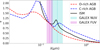 |
Fig. C.1 Dashed red: dust extinction curve for O-rich AGB stars (provided by DUSTY). Dashed blue: dust extinction curve for C-rich AGB stars (provided by DUSTY). Solid black: ISM extinction law from Gordon et al. (2023). The effective wavelengths and filter widths of the GALEX bands are represented as dotted lines and shadowed areas (cyan and magenta respectively). The three curves are scaled to match in the GALEX FUV band. |
Fig C.3 shows the comparison between RFUV/NUV and the UV excesses. It also shows linear fits between these parameters. There is a weak correlation (r=0.39) between RFUV/NUV and the NUV excess, which becomes stronger (r=0.62) after correcting for the dust attenuation. In contrast, the correlation between RFUV/NUV and the FUV excess is strong (r=0.85) and becomes even stronger (r=0.89) after the correction. This correlation shows that RFUV/NUV is a good tracer of UV excesses and can be used independently to explore trends.
This result is expected because small UV excesses indicate a larger contribution of the stellar component to RFUV/NUV, and stellar photospheric emission is characterised by low RFUV/NUV. As described in Sect. 1, both UV excesses and RFUV/NUV are related to the nature of the UV emission: small UV excesses and RFUV/NUV indicate an intrinsic origin (i.e. chromospheric activity), whereas large UV excesses and RFUV/NUV indicate an extrinsic origin (i.e. accretion activity). We highlight that these correlations can be seen despite the scatter produced by UV emission variability, and they become more pronounced when corrected for dust attenuation.
Appendix D SEDs and best-fit models for the rest of dusty AGB stars
Fig. D.1 shows the SEDs and their best-fit DUSTY models for the rest of dusty AGB stars to complement the sources already shown in Fig. 1.
Appendix E Parameter uncertainties and correlations from the SED modelling
We present a detailed description of the procedure used to estimate the uncertainties of the free parameters used in the SED modelling and identify correlations between them. Single parameter uncertainties were estimated as 68% confidence intervals from the normalised log-likelihood distribution ln(L(x)). We defined the χ2 likelihood function as:
 (E.1)
(E.1)
where x are the free parameters. On the other hand, we explore degeneracies between pairs of parameters from their χ2 distributions. This method allowed us to identify which parameters are degenerated and visualise the degree to which these degeneracies affect the χ2 value.
Fig. E.1 shows the corner plot obtained for EY Hya as an example of the estimation of the uncertainties associated with the free parameters from the SED modelling and the identification of the correlations between them. We found the following sets of positive correlations: T* -τ, Tinn -τ, Tinn - Y, n -τ, and n - Y. On the other hand, we found the following set of anticorrelations: T* -Tinn, Tinn -n, and τ- Y.
These correlations are quite linear in these ranges of the parameters, although there are two exceptions: (i) log(Y) that presents non-linearities with n and τ550 and (ii) T* that presents sharp upper limits, this limit is related with an emission excess in optical wavelengths that cannot be compensated by the rest of parameters. Similar correlations were found for the rest of dusty sources and can be generalised for the modelling procedure.
Appendix F Comparison with NESS sample
We present a complementary comparison with the Nearby Evolved Stars Survey (NESS, Scicluna et al. 2022), which contains 485 nearby AGB stars. We first compared the CO(J=2-1) and IRAS 60 μm fluxes between our sample and NESS (obtained from Wallström et al. 2025) to check whether uvAGBs have statistically lower CO intensity at similar IRAS 60 μm as suggested by Alonso-Hernández et al. (2024) using the CO( J =1-0).
Fig. F.1 shows the comparison between CO(J=2-1) integrated intensity and IRAS 60 μm flux. We used the CO(J=2-1) intensities as they are available for both our sample and NESS. We scaled NESS CO(J=2-1) intensities to match our intensities for the three commonly detected in CO in both samples (R LMi, SV Peg and W Peg).
In the case of unresolved and optically thin envelopes the CO intensity is proportional to the infrared flux (i.e. slope of 1 in logarithmic scale). Nevertheless, we noted that some scattering in this relationship is expected due to optically depth, partially resolved sources and ISM pollution. We found that our uvAGBs with the largest IRAS 60 μm fluxes in our sample overlap with the trend described by NESS sources. However, our sources with lowest IRAS 60 μm fluxes are systematically under this trend, although they fall outside the IRAS 60 μm range covered by NESS. The resulting fits indicate that our sources have indeed lower CO( J=2-1) intensities as well as CO( J =1-0), as previously inferred by Alonso-Hernández et al. (2024).
We also compared the correlations that we found in Fig. 7 for the gas-to-dust ratio with (i) the ratio between CO and IRAS 60 μm and (ii) with RFUV/NUV. Our δ estimates are in the upper part of those covered by NESS, although this parameter depends in the methodology to estimate the mass-loss rates and it is sensitive to systematic effects. In the case of RFUV/NUV, we used the values without dust attenuation correction because we do not have the dust optical depths for the NESS sources.
Fig. F.2 shows the comparison between the gas-to-dust ratio and the ratio between CO and IRAS 60 μm and RFUV/NUV . It is shown that δ correlates with the ratio between CO and infrared emission, although some outliers (likely related with pollution in the IRAS 60 μm images) are present. We noted that δ is not a empirical value and depends on the employed assumptions and methodology. Therefore, it is likely the presence of some systematic differences between our δ estimates and NESS. On the other hand, δ anticorrelates with RFUV/NUV, although it presents some scatter that can be related with UV emission variability and it is not corrected from dust attenuation.
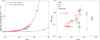 |
Fig. C.2 Left : Comparison between the opacity correction factor for the RFUV/NUV ratio and the opacity at the fiducial wavelength. The dashed and dash-dotted lines represents the correlations of |


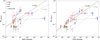 |
Fig. C.3 Correlations between RFUV/NUV and the NUV and FUV excesses (left and right respectively). The colour and shape of the markers represent the stellar variability and chemistry type as in Fig. 4. Grey markers are those without correction from dust attenuation. The dotted lines link the markers for the same sources before and after the dust attenuation correction. The dashed lines represents linear fits to the points. |
Finally, we crossmatched the NESS catalogue with GALEX and found that among the 485 AGB stars in NESS, 163 were detected in the NUV band and 95 were also detected in the FUV band. These percentages illustrate that large AGB star samples also contain some uvAGBs.
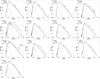 |
Fig. D.1 Same as Fig. 1, but for the rest of dusty AGB stars in the sample. In the case of VY UMa, the solid diamonds and the dashed magenta line represent respectively the fluxes and the DUSTY model for the detached shell. |
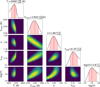 |
Fig. E.1 Corner plot of EY Hya to exemplify correlations between the different free parameters. The 1D curves display the log-likelihood functions, the solid red line indicates the most likely value and the dashed red lines and shadowed region the ±1σ values. The 2D histograms display the χ2 distributions, the dashed red and black lines indicate the areas with values lower than χ2+1 and χ2+2 respectively. |
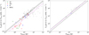 |
Fig. F.1 Comparison of CO(J=2-1) with IRAS 60 μm for O-rich and C-rich AGB stars (left and right respectively). The colour and shape of the markers represent the stellar variability and chemistry type as in Fig. 4. Empty triangles are upper limits for the CO( J=2-1) intensities. Grey markers represent NESS sources. The solid black lines indicates the equality relationship between CO(J=2-1) intensity and IRAS 60 μm fluxes. The dashed lines represents linear fits to the points, solid and purple for our sample and NESS respectively. |
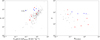 |
Fig. F.2 Comparison of the gas-to-dust ratio with the ratio between CO( J=2-1) and IRAS 60 μm and RFUV/NUV (left and right respectively). The colour and shape of the markers represent the stellar variability and chemistry type as in Fig. 4. Empty triangles are upper limits for the CO( J=2-1) intensities. Grey markers represent NESS sources. The values of RFUV/NUV shown in this figure were not corrected from dust attenuation. It can be appreciated a correlation and an anticorrelation in the figures on the left and right respectively. |
All Tables
All Figures
|
Fig. 1 SEDs and best-fit DUSTY models for the dusty AGB stars. Solid blue line: input spectra; solid red line: total DUSTY model; dotted cyan line: attenuated input spectral component; dashed green line: dust scattered component; dot-dashed orange line: dust thermal component. Photometric fluxes are indicated as filled circles (in a few cases the variability-induced uncertainties are larger than the average value), photometric data not included in the analysis as empty circles, and upper limits as empty triangles. Solid grey lines are GAIA, IRAS, and ISO spectra; shadowed areas indicate 10% uncertainties. |
| In the text | |
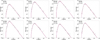 |
Fig. 2 Same as Fig. 1, but for ‘naked’ sources. |
| In the text | |
|
Fig. 3 Histograms showing the distributions of the best-fit solution SED modelling parameters. From left to right: stellar effective temperature, dust inner radius temperature, density power-law index, dust shell radial optical depth at 550 nm. White bins represent ‘naked’ O-rich uvAGBs, grey bins represent O-rich uvAGBs with dust component, and striped bins represent C-rich uvAGBs. |
| In the text | |
|
Fig. 4 HRD of our the sample. The size of the markers is proportional to the dust shell masses as shown in the bottom right legend. The marker’s colour represents the variability type. Red: semi-regulars (SRs), green: irregulars (LB), and blue: Miras (M). The shape of the markers represents the chemistry of the AGB stars. Circles: O-rich (‘naked’ as asterisks), crosses: C-rich. |
| In the text | |
|
Fig. 5 Comparison of the best-fit solution SED modelling parameters (from top to bottom : T*, Tinn, n and τ550) with P (left) and |
| In the text | |
|
Fig. 6 Comparison between the gas and dust mass-loss rates for our sample of uvAGBs. The colour and shape of the markers represent the stellar variability and chemistry type as in Fig. 4. Grey markers represent sources from the NESS sample. The dashed line represents the relationship presented in Wallström et al. (2025). The histograms at the top and to the right of the figure indicate the distribution of Ṁdust and Ṁgas respectively. |
| In the text | |
|
Fig. 7 Comparison between the gas-to-dust ratio and different parameters (from left to right : ratio of CO J=2-1 velocity-integrated line flux to the IRAS 60 μm flux, Ṁgas, P, and |
| In the text | |
|
Fig. A.1 Radial surface brightness profiles at 70 μm (left) and 160 μm (right) for the four semi-extended sources in the sample (from top to bottom : RU Her, SV Peg, TDra and VEri). Solid circles correspond to Herschel/PACS radial surface brightness profiles, dashed lines to DUSTY synthetic images convolved with their respective PSFs and dotted lines to the PSFs to represent point-source radial surface brightness. |
| In the text | |
|
Fig. B.1 Adopted density profile for VY UMa. The solid black line represents the modified density distribution to fit the detached shell. The dotted red line represents the smooth density profile from the presentday mass-loss. The green area represent the location of the detached shell in the Herschel/PACS images. |
| In the text | |
|
Fig. B.2 Left : Herschel/PACS images of VYUMa. The solid cyan represents the aperture used to isolate the central component (representing the present-day mass-loss), and the dashed cyan lines the aperture used to measure the extended detached shell. Right : Radial surface brightness profiles, the markers indicate the surface brightness from the images, the dashed line the surface brightness from DUSTY models convolved with their respective Herschel/PACS PSFs, and the dotted lines the Herschel/PACS PSFs. |
| In the text | |
|
Fig. C.1 Dashed red: dust extinction curve for O-rich AGB stars (provided by DUSTY). Dashed blue: dust extinction curve for C-rich AGB stars (provided by DUSTY). Solid black: ISM extinction law from Gordon et al. (2023). The effective wavelengths and filter widths of the GALEX bands are represented as dotted lines and shadowed areas (cyan and magenta respectively). The three curves are scaled to match in the GALEX FUV band. |
| In the text | |
|
Fig. C.2 Left : Comparison between the opacity correction factor for the RFUV/NUV ratio and the opacity at the fiducial wavelength. The dashed and dash-dotted lines represents the correlations of |
| In the text | |
|
Fig. C.3 Correlations between RFUV/NUV and the NUV and FUV excesses (left and right respectively). The colour and shape of the markers represent the stellar variability and chemistry type as in Fig. 4. Grey markers are those without correction from dust attenuation. The dotted lines link the markers for the same sources before and after the dust attenuation correction. The dashed lines represents linear fits to the points. |
| In the text | |
|
Fig. D.1 Same as Fig. 1, but for the rest of dusty AGB stars in the sample. In the case of VY UMa, the solid diamonds and the dashed magenta line represent respectively the fluxes and the DUSTY model for the detached shell. |
| In the text | |
|
Fig. E.1 Corner plot of EY Hya to exemplify correlations between the different free parameters. The 1D curves display the log-likelihood functions, the solid red line indicates the most likely value and the dashed red lines and shadowed region the ±1σ values. The 2D histograms display the χ2 distributions, the dashed red and black lines indicate the areas with values lower than χ2+1 and χ2+2 respectively. |
| In the text | |
|
Fig. F.1 Comparison of CO(J=2-1) with IRAS 60 μm for O-rich and C-rich AGB stars (left and right respectively). The colour and shape of the markers represent the stellar variability and chemistry type as in Fig. 4. Empty triangles are upper limits for the CO( J=2-1) intensities. Grey markers represent NESS sources. The solid black lines indicates the equality relationship between CO(J=2-1) intensity and IRAS 60 μm fluxes. The dashed lines represents linear fits to the points, solid and purple for our sample and NESS respectively. |
| In the text | |
|
Fig. F.2 Comparison of the gas-to-dust ratio with the ratio between CO( J=2-1) and IRAS 60 μm and RFUV/NUV (left and right respectively). The colour and shape of the markers represent the stellar variability and chemistry type as in Fig. 4. Empty triangles are upper limits for the CO( J=2-1) intensities. Grey markers represent NESS sources. The values of RFUV/NUV shown in this figure were not corrected from dust attenuation. It can be appreciated a correlation and an anticorrelation in the figures on the left and right respectively. |
| In the text | |
Current usage metrics show cumulative count of Article Views (full-text article views including HTML views, PDF and ePub downloads, according to the available data) and Abstracts Views on Vision4Press platform.
Data correspond to usage on the plateform after 2015. The current usage metrics is available 48-96 hours after online publication and is updated daily on week days.
Initial download of the metrics may take a while.