| Issue |
A&A
Volume 700, August 2025
|
|
|---|---|---|
| Article Number | A17 | |
| Number of page(s) | 17 | |
| Section | Cosmology (including clusters of galaxies) | |
| DOI | https://doi.org/10.1051/0004-6361/202453562 | |
| Published online | 25 July 2025 | |
The imprint of cosmic voids from the DESI Legacy Survey DR9 Luminous Red Galaxies in the Planck 2018 lensing map through spectroscopically calibrated mocks
1
Aix Marseille Univ, CNRS/IN2P3, CPPM, Marseille, France
2
MTA-CSFK Lendület “Momentum” Large-Scale Structure (LSS) Research Group, 1121 Konkoly Thege Miklós út 15-17, Budapest, Hungary
3
Konkoly Observatory, HUN-REN CSFK, MTA Centre of Excellence, Budapest, Konkoly Thege Miklós út 15-17 H-1121, Hungary
4
Brookhaven National Laboratory, Physics Department, Upton, NY 11973, USA
5
Physics Dept., Boston University, 590 Commonwealth Avenue, Boston, MA 02215, USA
6
Dipartimento di Fisica “Aldo Pontremoli”, Università degli Studi di Milano, Via Celoria 16, I-20133 Milano, Italy
7
Department of Physics & Astronomy, University College London, Gower Street, London WC1E 6BT, UK
8
IRFU, CEA, Université Paris-Saclay, F-91191 Gif-sur-Yvette, France
9
Lawrence Berkeley National Laboratory, 1 Cyclotron Road, Berkeley, CA 94720, USA
10
Instituto de Física, Universidad Nacional Autónoma de México, Circuito de la Investigación Científica, Ciudad Universitaria, Cd. de México C. P. 04510, Mexico
11
Departamento de Física, Universidad de los Andes, Cra. 1 No. 18A-10, Edificio Ip, CP 111711 Bogotá, Colombia
12
Observatorio Astronómico, Universidad de los Andes, Cra. 1 No. 18A-10, Edificio H, CP 111711 Bogotá, Colombia
13
Instituto de Fisica Teorica IFT-UAM/CSIC, Universidad Autonoma de Madrid, Cantoblanco, 28049 Madrid, Spain
14
Fermi National Accelerator Laboratory, PO Box 500 Batavia, IL 60510, USA
15
Center for Cosmology and AstroParticle Physics, The Ohio State University, 191 West Woodruff Avenue, Columbus, OH 43210, USA
16
Department of Physics, The Ohio State University, 191 West Woodruff Avenue, Columbus, OH 43210, USA
17
The Ohio State University, Columbus, 43210 OH, USA
18
Department of Physics, Southern Methodist University, 3215 Daniel Avenue, Dallas, TX 75275, USA
19
Department of Physics and Astronomy, University of California, Irvine 92697, USA
20
NSF NOIRLab, 950 N. Cherry Ave., Tucson, AZ 85719, USA
21
Institució Catalana de Recerca i Estudis Avançats, Passeig de Lluís Companys, 23, 08010 Barcelona, Spain
22
Institut de Física d’Altes Energies (IFAE), The Barcelona Institute of Science and Technology, Campus UAB, 08193 Bellaterra Barcelona, Spain
23
Department of Physics and Astronomy, Siena College, 515 Loudon Road, Loudonville, NY 12211, USA
24
Department of Physics & Astronomy and Pittsburgh Particle Physics, Astrophysics, and Cosmology Center (PITT PACC), University of Pittsburgh, 3941 O’Hara Street, Pitts- burgh, PA 15260, USA
25
Departament de Física, EEBE, Universitat Politècnica de Catalunya, c/Eduard Maristany 10, 08930 Barcelona, Spain
26
Instituto de Astrofísica de Andalucía (CSIC), Glorieta de la Astronomía, s/n, E-18008 Granada, Spain
27
Department of Physics and Astronomy, Sejong University, Seoul 143-747, Korea
28
CIEMAT, Avenida Complutense 40, E-28040 Madrid, Spain
29
University of Michigan, Ann Arbor, MI 48109, USA
⋆ Corresponding author.
Received:
20
December
2024
Accepted:
14
April
2025
Abstract
The cross-correlation of cosmic voids with the lensing convergence (κ) map of the Cosmic Microwave Background (CMB) fluctuations provides a powerful tool to refine our understanding of the current cosmological model. However, several studies have reported a moderate tension (up to ∼2σ) between the lensing imprint of cosmic voids on the observed CMB and the ΛCDM signal predicted by simulations. To address this “lensing-is-low” tension and to obtain new, precise measurements of the signal, we exploit the large DESI Legacy Survey Luminous Red Galaxy (LRG) data set, covering approximately 19 500 deg2 of the sky and including about 10 million LRGs at z < 1.05. Our ΛCDM template was created using the Buzzard mocks, which we specifically calibrated to match the clustering properties of the observed galaxy sample by exploiting more than one million DESI spectra. We identified our catalogs of 3D voids in the range 0.35 < z < 0.95 and cross-correlated them through a stacking methodology, dividing the sample into bins according to the redshift and λv values of the voids. For the full void sample, we report a 14σ detection of the lensing signal, with Aκ = 1.016 ± 0.054, which increases to 17σ when considering the void-in-void (Aκ = 0.944 ± 0.064) and the void-in-cloud (Aκ = 0.975 ± 0.060) populations individually, the highest detection significance for studies of this kind. We observe a full agreement between observations and ΛCDM mocks across all redshift bins, sky regions, and void populations considered. In addition to these findings, our analysis highlights the importance of accurately matching sparseness and redshift error distributions between mocks and observations, as well as the role of λv in enhancing the signal-to-noise ratio through void population discrimination.
Key words: cosmic background radiation / cosmological parameters / cosmology: observations / large-scale structure of Universe
© The Authors 2025
 Open Access article, published by EDP Sciences, under the terms of the Creative Commons Attribution License (https://creativecommons.org/licenses/by/4.0), which permits unrestricted use, distribution, and reproduction in any medium, provided the original work is properly cited.
This article is published in open access under the Subscribe to Open model. This email address is being protected from spambots. You need JavaScript enabled to view it. to support open access publication.
1. Introduction
The past 25 years have radically transformed our perception and ability to study the cosmos. Observation of distant Type Ia supernovae (Riess et al. 1998; Schmidt et al. 1998; Perlmutter et al. 1999), observations of large-scale structures, and anisotropies of the cosmic microwave background (CMB; Eisenstein et al. 2005; Komatsu et al. 2011; Bennett et al. 2013; Planck Collaboration VI 2020) have introduced and confirmed the model of an accelerating Universe. In addition, the remarkable technological advancements have enabled the development of a new generation of wide- and deep-field observational surveys (York et al. 2000, The Dark Energy Survey Collaboration 2005 as key examples of the first major surveys of this kind), complemented by cosmological simulations of unprecedented scale and resolution.
These cutting-edge observational techniques have enabled mapping the large-scale distribution of matter, revealing a Universe composed of overdense sheets and filaments interspersed with vast underdensities, known as cosmic voids (Gregory & Thompson 1978; Jõeveer et al. 1978; Kirshner et al. 1981; de Lapparent et al. 1986). Collectively, these intricate structures form what is widely referred to as the cosmic web.
Cosmic voids dominate the late Universe in terms of volume. Although lacking a universally agreed upon definition, these structures can be characterized as vast, underdense regions of space that, when isolated, evolve over time by transferring matter from their central regions to the surrounding filaments and overdense walls.
Thanks to their unique environmental characteristics, voids have emerged as fundamental resources for assessing the validity of the Lambda-Cold Dark Matter (ΛCDM) model and exploring scenarios of modified gravity (Clampitt et al. 2013; Spolyar et al. 2013; Cai et al. 2015; Zivick & Sutter 2016; Baker et al. 2018; Perico et al. 2019; Contarini et al. 2021; Wilson & Bean 2023; Mauland et al. 2023), massive neutrinos (Massara et al. 2015; Banerjee & Dalal 2016; Kreisch et al. 2019; Schuster et al. 2019; Mauland et al. 2023; Vielzeuf et al. 2023; Thiele et al. 2024), primordial non-Gaussianities (Chan et al. 2019), among other phenomena beyond the standard model of particle Physics (see Pisani et al. 2019 and Moresco et al. 2022 for extensive reviews).
The constraining power of cosmic voids emerges from a variety of probes. Examples include the void size function (Sheth & van de Weygaert 2004; Jennings et al. 2013; Pisani et al. 2015; Contarini et al. 2019, 2023; Ronconi et al. 2019; Correa et al. 2022; Pelliciari et al. 2023; Song et al. 2024; Verza et al. 2024), which represents the number of voids as a function of their radius, and the void-galaxy cross-correlation function, which provides information on the density profile of voids and the distribution of mass within them (Hamaus et al. 2014a; Schuster et al. 2023, 2024). This cosmological exploitation relies on modeling dynamical and geometrical distortions under the assumption of the average spherical shape of voids (Ryden 1995; Lavaux & Wandelt 2012; Sutter et al. 2012, 2014; Paz et al. 2013; Hamaus et al. 2014b,a, 2015; Hamaus et al. 2022; Nadathur & Percival 2019; Correa et al. 2022; Aubert et al. 2022; Correa & Paz 2022; Woodfinden et al. 2022, 2023; Mauland et al. 2023; Radinović et al. 2023, 2024; Fraser et al. 2024). Additional and more recent probes come from velocity profiles (Paz et al. 2013; Zivick et al. 2015; Hamaus et al. 2016; Massara et al. 2022; Wilson & Bean 2023), the void autocorrelation function (Chan et al. 2014; Hamaus et al. 2014b; Clampitt et al. 2016), power-spectrum (Bonici et al. 2023), weak lensing (Melchior et al. 2014; Barreira et al. 2015; Sánchez et al. 2017, Baker et al. 2018; Hossen et al. 2022; Boschetti et al. 2024), as well as the shape and ellipticity of voids (Lee & Park 2009; Zivick et al. 2015; Rezaei 2020; Schuster et al. 2023).
The large-scale matter distribution in the Universe alters the CMB and introduces anisotropies therein (Sachs & Wolfe 1967; Sunyaev & Zeldovich 1970; Blanchard & Schneider 1987; Kashlinsky 1988; Cole & Efstathiou 1989; Sasaki 1989; Tomita & Watanabe 1989; Linder 1990). Analogously to their overdense counterparts, cosmic voids induce various effects on the observed CMB. These effects provide unique additional probes to test the cosmological model. While the presence of gas modifies the energy of CMB photons, via the thermal Sunyaev-Zel’dovich effect (tSZ; Sunyaev & Zeldovich 1970), the temporal variation of the gravitational potential due to the accelerated expansion of the Universe introduces temperature anisotropies that can be used to test the effects of dark energy (Integrated Sachs-Wolfe effect, ISW; Sachs & Wolfe 1967). Illustrative examples of the ISW effect within cosmic voids are provided by Nadathur et al. (2012), Ilić et al. (2013), Cai et al. (2014), Kovács (2018), and Naidoo et al. (2024). Similarly, examples of the tSZ effect within voids are discussed by Alonso et al. (2018), Li et al. (2020), and Li et al. (2024).
The imprint of cosmic voids on the CMB lensing signal offers a unique probe of the underlying total matter distribution. Unlike clusters and filaments, cosmic voids induce a demagnification effect on the CMB, resulting from the deflection of photons as they cross these underdense regions. This effect is observed as a negative signal in the CMB convergence (κ) maps. Despite the complexity of measuring the lensing signal from an individual void due to dominant noise amplitude in CMB lensing maps at typical scales, numerous stacked measurements have been conducted in recent years. These studies report significance values ranging from ∼3σ to ∼13σ (Cai et al. 2014; Raghunathan et al. 2020; Vielzeuf et al. 2021; Hang et al. 2021; Kovács et al. 2022; Camacho-Ciurana et al. 2024; Demirbozan et al. 2024), highlighting the effectiveness of stacking techniques in isolating the CMB lensing signal induced by voids from background noise.
However, several recent studies have reported moderate tensions, up to ∼3σ, between the observed signal amplitudes and predictions from ΛCDM simulations (Vielzeuf et al. 2021; Hang et al. 2021; Kovács et al. 2022; Camacho-Ciurana et al. 2024). These discrepancies depend on factors such as void identification strategies employed, the degree of smoothing applied to the CMB lensing maps, and the specific sub-populations of voids considered. In light of these tensions, and considering recent analyses of weak lensing of the Dark Energy Spectroscopic Instrument (DESI; DESI Collaboration 2016a,b) Luminous Red Galaxy (LRG) sample (Chen et al. 2024), which have addressed some of the existing lensing tensions through innovative treatment of systematics, it is crucial to thoroughly understand the nature of these disagreements with ΛCDM simulated predictions. This understanding is essential to properly assess the systematics associated with voids and may provide further insight into the discrepancies observed within the ΛCDM model.
The purpose of this study is to exploit the large catalog of voids identified in the photometric LRG population of the DESI Legacy Imaging Surveys (Dey et al. 2019) to investigate current tensions in literature. We measure the cross-correlation with CMB lensing from Planck 2018 and compare the amplitude of the signal with those obtained from the Buzzard mocks (DeRose et al. 2019), which we designed and adapted to match our observations by analyzing and correcting a number of possible systematics. The paper is organized as follows. In Sect. 2, we introduce our observed and simulated data sets. Section 3 describes the adaptation and validation of our mocks and provides a description of our stacking methodology and error analysis. We present and discuss the main observational results of this paper in Sect. 4. Finally, Sect. 5 summarizes our conclusions.
2. Data sets
2.1. DESI legacy surveys DR9 luminous red galaxies
We identified our cosmic void sample by exploiting the LRG population extracted from the ninth Data Release (DR9; Schlegel et al. 2021) of the DESI Legacy Imaging Surveys (see Zhou et al. 2023 for further details on the LRG catalog and the selection process).
The Legacy Surveys were designed to enable target selection for the DESI Survey and consist of a mosaic of three different observational projects, as shown in Fig. 1. The Northern Hemisphere was mapped by a combination of different surveys: the sky area with Dec ≥ + 32.735° (J2000 coordinates) was observed by the Mayall z-band Legacy Survey (MzLS; Silva et al. 2016), using the MOSAIC-3 camera at the prime focus of the 4-meter Mayall telescope at Kitt Peak National Observatory, and the Beijing–Arizona Sky Survey (BASS; Zou et al. 2017), which used the 90Prime camera at the prime focus of the Bok 2.3-m telescope. The Dark Energy Camera (DECam; Flaugher et al. 2015) on the Blanco 4m telescope, located at the Cerro Tololo Inter-American Observatory, provided observations of the remaining two-thirds of the survey footprint. In particular, the Dark Energy Camera Legacy Survey (DECaLS; Blum et al. 2016) completed the observations of the North Galactic Cap, covering the region with Dec ≤ + 32.375°, and observed the equatorial regions of the South Galactic Cap. The remaining part of the Southern hemisphere was integrated by the Dark Energy Survey (DES; The Dark Energy Survey Collaboration 2005) which previously used the same instrument to map around 5000 deg2 of the South sky. The Legacy Survey DR9 also included fluxes from the all-sky Wide-Field Infrared Survey Explorer (WISE, Wright et al. 2010) at the locations of Legacy Surveys optical sources. The exploited LRG sample, selected using g, r, z, and W1 photometry from the DESI Legacy Imaging Surveys, is highly robust against imaging systematics. With a comoving number density of 5 × 10⁻⁴ h3Mpc−3 in 0.4 < zph < 0.8, this sample has significantly higher density than previous LRG surveys, such as the SDSS Legacy survey (Margon 1999), BOSS (Dawson et al. 2013), and eBOSS (Dawson et al. 2016). The total observed sky area of 19 573 deg2, combined with the high comoving number density, allowed us to exploit a total of 10 402 494 LRGs in the redshift range 0.30 < zph < 1.05.
 |
Fig. 1. Footprints of the MzLS+BASS, DECaLS, and DES surveys that compose the DESI Legacy Survey, covering a total observed sky area of 19 573 deg2. |
The selected sample was supplemented with 1 005 750 spectroscopic redshifts from DESI, particularly from the first phase of Survey Validation (SV1), the one-percent survey (SV3; covering 1% of the final area), and the first two months of the Main Survey.
2.2. CMB convergence map from Planck mission DR2018
The convergence κ, our observable, is defined as the ratio
 (1)
(1)
where Σ is the projected density along the line of sight θ. The critical projected density Σcr, for a lens located between the observer and the last scattering surface of the CMB, is defined as
 (2)
(2)
where rcmb is the distance between the observer and the CMB and r as the distance between the observer and the lens. Assuming the classical Poisson equation for the gravitational potential, Φ(r, θ)
 (3)
(3)
we obtain a formulation for Σ:
 (4)
(4)
Substituting Eqs. (2) and (4) in Eq. (1), we find
 (5)
(5)
Using the cosmological formulation of the Poisson equation for the gravitational,
 (6)
(6)
where δ(r, θ) is the local density contrast, we recover the equation for κ(θ), estimated from the matter density field δ(r, θ), in the Born approximation with the Hubble constant H0 and the matter density parameter Ωm made explicit:
 (7)
(7)
For our analysis, we used the publicly available reconstructed CMB lensing convergence (κ) map provided by the Planck collaboration (data release 2018; see Planck Collaboration VIII 2020). The map was reconstructed using the minimum-variance quadratic estimator (Hu & Okamoto 2002), which combines CMB temperature and polarization data and is provided in the form of harmonic coefficients κlm up to lmax, mmax = 2048.
Despite the potential for higher resolution, we generated a HEALpix1 (Górski et al. 2005) map with Nside = 512 and lmax, mmax = 1536. These choices yield a HEALpix map and angular power spectrum resolution of approximately θ ∼ 7 arcmin, ensuring sufficient accuracy relative to the angular dimensions of the analyzed structures and precision in generating the random CMB maps used for error estimation (see Sect. 3.4 for further details). We verified that increasing the resolution does not significantly improve our results while imposing a high computational cost.
Finally, a Gaussian smoothing was applied to the map to suppress noise at small scales and improve the signal-to-noise ratio (S/N). Unlike some previous works (Vielzeuf et al. 2021; Kovács et al. 2022; Camacho-Ciurana et al. 2024) that employ a Gaussian smoothing with FWHM = 1.0°, we opted for a more conservative filter with FWHM = 0.5°. This approach maximizes the measured signal while preserving the imprint of smaller voids on the CMB, whose angular radii often measure less than 1.0°. We note, however, that the smoothing amplitude can modify and enhance potential tensions between the measured signal and the simulated templates. In the future, a more in-depth investigation of the smoothing effect at different scales will be conducted in the future, particularly if new tensions are detected. The CMB lensing map, along with the extents of the North and South regions, is shown in Fig. 2.
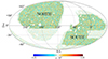 |
Fig. 2. Planck CMB lensing map, smoothed with a Gaussian filter of FWHM = 0.5°. The DESI Legacy Survey footprint is overlaid, indicating the region where voids are identified and cross-correlations are performed. The footprint is divided into North and South regions, corresponding to the North and South Galactic Caps. CMB regions with negative and positive convergence values are represented by the blue and red ranges of the color palette, respectively. |
2.3. Buzzard mocks: simulated galaxies and CMB convergence map
The Buzzard mocks are a suite of quarter-sky galaxy catalogs constructed from N-body lightcone simulations using Addgals (Wechsler et al. 2022), an algorithm designed to reproduce the clustering properties of subhalo abundance matching models (DeRose et al. 2022) in low-resolution lightcone simulations. The underlying N-body simulations were run with L-Gadget2, a streamlined version of Gadget2 (Springel 2005) optimized for large N-body simulations and initialized with second-order Lagrangian perturbation theory at z = 49 using 2LPTIC (Crocce et al. 2006). The linear power spectrum was generated using CAMB (Lewis & Bridle 2002) assuming a ΛCDM cosmology with Ωm = 0.286, Ωb = 0.046, ns = 0.96, h = 0.7, σ8 = 0.82, Ωr = 0, and Ων = 0. Each lightcone simulates a quarter of the sky up to z = 2.34 and is constructed from three different simulation boxes, with Lbox = {1050, 2600, 4000} h−1 Mpc and 14003, 20483, and 20483 particles, respectively for z ∈ [0.0, 0.34),[0.34, 0.9),[0.9, 2.34). Each realization assumes the same cosmological parameters, but varies the white noise field used to initialize the simulations.
Galaxy catalogs were generated using Addgals, which assigns each galaxy to a particle in the lightcone simulations, imbuing them with positions, velocities, and spectral energy distributions (SEDs) that can be integrated to provide broadband photometry. DESI-like LRG catalogs were selected using slightly modified versions of the color cuts applied to the DESI Legacy Survey data (DeRose et al. in prep.):
 (8)
(8)
where c1 = 0.4 and c2 = 0.275 are the differences in color cuts from the DESI targeting cuts, adjusted to roughly match the angular target density of the DESI LRG sample.
Photometric redshifts were then generated by fitting a model for σ(zph|zsp) to the DESI Legacy Survey data and applying Gaussian errors to the true redshifts of each simulated LRG. Finally, CMB lensing maps were produced by applying the Born approximation to 50 h−1Mpc thick density shells measured from the lightcone simulations. In this work we used four realizations of the Buzzard mocks.
3. Methods
3.1. Validation and calibration of mocks
To evaluate the lensing imprint of our cosmic void sample on the CMB and investigate and any potential deviations from the ΛCDM simulated predictions, we compared the observed cross-correlation signal with a ΛCDM template derived from mocks through a template-fitting process. The lensing imprint we measured depended strongly on our void population, which, in turn, was inherently linked to the characteristics of the galaxy sample. Consequently, it was crucial that the simulated galaxy populations shared the same intrinsic properties as the observed sample. To address potential systematic errors arising from discrepancies between the simulated and observed LRG data sets, we evaluated two key factors affecting void identification: photometric error and sparseness. Comparing two equally biased galaxy populations with identical photometric properties and mass distributions but differing in either sparseness or redshift error distributions can lead to markedly different void populations. Identical galaxy samples with differing photometric redshift (zph) errors resulted in voids with varying degrees of contamination from galaxies whose redshifts had been inaccurately determined. This contamination particularly affected the estimation of the inner density contrast, thereby impacting both the identification and size of the voids. Conversely, different levels of sparseness significantly influenced the resolution of the void-finding method, thereby affecting the void size function. It was evident that distinct void populations exhibited different lensing properties.
3.1.1. Photometric redshift correction
As a first step of our analysis, we examined the distribution of the photometric redshift errors. We prioritized this aspect because modifications to the photometric redshift distribution in the mocks would subsequently affect the sparseness. We utilized both photometric and spectroscopic redshift (zsp) data, available for the mock populations and approximately 10% of the observed galaxies, to estimate photometric errors, considering spectroscopic redshifts as the true redshift values. The matching between spectroscopic and photometric redshifts of our sources allowed us to correct the photometric redshifts assigned to galaxies in the mocks, thereby estimating a new and more precise photometric redshift distribution. To account for potential variations in the error distribution as a function of true redshift, we divided our sample into 75 bins with Δz = 0.01. For each redshift bin, we calculated the distribution of the redshift error zerr = zsp − zph, and then determined the cumulative distribution function (CDF), normalized between 0 and 1. This CDF gives the probability that zerr, i < z⋆, where z⋆ represents a specific value within the distribution.
At this stage, we extracted a set of random numbers R from a uniform distribution between 0 and 1, matching the size of our LRG catalog for each mock realization. Each mock galaxy was then assigned a redshift error 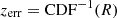 . The new photometric redshift for each mock galaxy was then straightforwardly recovered as zph, i = zsp, i − zerr, i.
Figure 3 shows the redshift error distributions for the observed data set and one Buzzard realization at the 68.27th, 95.45th, and 99.73th percentiles. It is evident that not only do the two distributions exhibit significantly different standard deviations, they also diverge substantially in their overall trends.
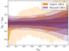 |
Fig. 3. Redshift error distributions for the observed and one simulated LRG data sets, shown in orange and purple, respectively, at the 68.27th, 95.45th, and 99.73th percentiles. Darker shades represent smaller percentile ranges. The two distributions exhibit distinct trends and deviations from zero, which must be corrected to ensure proper matching between observations and mocks. |
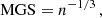
Figure 4 shows the Mean Galaxy Separation (MGS), indicator of the sparseness of the sample, defined as
 (9)
(9)
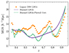 |
Fig. 4. Redshift evolution of the MGS observed in the Legacy Survey (orange dots) compared with the MGSs of the four Buzzard mock realizations before (purple lines) and after (green lines) photometric redshift correction. The shape change after correction, now matching the MGS trend of the Legacy Survey galaxy sample, strongly indicates the accuracy of the redshift calibration procedure. |
where n is the galaxy number density, for both the observed and simulated samples. Moreover, it illustrates how the MGS changes after the zph correction of the mocks. The post-correction shape matching of the two MGS distributions strongly indicates the success of the procedure.
3.1.2. Sparseness matching
In the second step of the mock validation and adaptation process, we corrected the sparseness of the simulated data sets to align with the observations. To account for the slight differences in sparseness between the different survey regions, we subdivided the observed data set into two regions, as shown in Fig. 2, and handled the North and South Galactic Caps separately.
Similar to the approach used for photometric redshift correction, we divided the samples into bins with Δz = 0.01. Within each bin, we randomly sampled our mock galaxy populations to match the number densities of the simulated and observed catalogs. This procedure was feasible only for redshift ranges where our mock data sets were denser than the observed ones. However, this condition was not consistently met for 0.35 < z < 0.50 and z > 0.80 (see Fig. 4). Despite the inability to fully match the sparseness in these redshift ranges, the density discrepancies between the different populations remained below 5%. This minimal discrepancy ensured that the impact of varying sparseness on void identification systematics was almost negligible.
We applied this procedure to our four mock realizations, for both the North and South observed catalogs, resulting in eight corrected simulated data sets (four for the North Galactic Cap and four for the South Galactic Cap).
Figure 5 shows the combined effect of the two correction procedures for both the North and South data sets, resulting in an almost perfect MGS match across the entire redshift range considered by this cosmological analysis. The slight difference in sparseness between the two regions arises from random fluctuations and minor observational differences between the surveys.
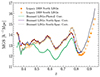 |
Fig. 5. Redshift evolution of the MGS observed in the Legacy Survey, measured in the North (orange dots) and South (white dots) regions. The observed MGS values are compared with those from the four redshift-calibrated Buzzard mock realizations before (purple lines) and then after sparseness correction, performed independently to match the North (green lines) and South (gray lines) regions. An almost complete match is observed between the observations and simulations, with only minor differences at z ∼ 0.4 and z > 0.8, where the mocks appear more sparse than the observations, making subsampling infeasible. |
3.2. Void finding
In recent decades, the lack of a precise theoretical definition of cosmic voids has led to the development of various void-finding algorithms. According to Lavaux & Wandelt (2010), these methods can be classified into three main categories: density-based, geometry-based, and dynamics-based, depending on how the algorithms exploit the mass tracer field (see Colberg et al. 2008 for an overview of void-finding methods and their systematics). Cosmic voids can be identified in 2D or 3D. Although 2D void identification has generally been more effective in maximizing the S/N for lensing analysis (see, e.g., Cautun et al. 2018), we opted for a 3D void catalog in our study. This choice allowed us to address tensions observed in previous work, particularly those involving 3D voids (see, i.e., Vielzeuf et al. 2021 and Camacho-Ciurana et al. 2024), and also helped mitigate issues related to the intrinsic alignment of voids, which can produce spurious lensing signals.
3.2.1. REVOLVER algorithm
For identifying our 3D voids, we used the REVOLVER2 (REal-space VOid Locations from surVEy Reconstruction) void-finding code (Nadathur et al. 2019) which is based on a modified version of the ZOBOV algorithm (Neyrinck 2008). The ZOBOV algorithm identifies cosmic voids in the minima of the reconstructed density field, which is achieved through a Voronoi tessellation.
The identification process is fully described in Nadathur et al. (2019), but can be summarized as follows. The three-dimensional space covered by the tracer catalog is subdivided via a Voronoi tessellation. To each tracer particle is assigned a unique Voronoi cell to each tracer particle, defined as the region closer to that particle than to any other. The density at any point within each cell is then determined by taking the inverse of the cell volume. To account for the survey mask, forbidden regions are populated with mock tracers, simulating overdense sections of space. Density minima in the Voronoi density field are then identified. A Voronoi cell is defined as a density minimum if its volume is larger than that of its neighboring cells. These minima constitute the initial seeds of the voids. From each density minimum, the algorithm merges adjacent cells with increasing density until no higher adjacent density cells remains. These merged regions, or basins, are referred to as zones, representing local depressions in the density field. A watershed transform then merges zones into larger voids. To preserve the underdense environment of voids, a merging condition is applied: the ridge between any two zones must be less than 20 percent of the average tracer density. This procedure creates a hierarchy of voids and subvoids. A full discussion of the watershed methods is provided in Platen et al. (2007).
The center of each void is defined as the circumcenter of the positions of the lowest-density galaxy in the void and its three lowest-density mutually adjacent neighbors. This is equivalent to defining the center of the largest empty sphere that can be inscribed within the void. Finally, the effective radius of each void, rv, is assigned from its total volume, calculated as the sum of the volumes of its constituent Voronoi cells, Vv = ∑iVi. The radius corresponds to that of a sphere with:
 (10)
(10)
Additionally, the code provides a set of void properties, including the central density contrast δv, the average density contrast  , and the parameter λv, a useful proxy for the gravitational potential at the void center (Nadathur et al. 2017), defined as
 (11)
(11)
The parameter λv plays a fundamental role in distinguishing void populations with varying internal potential values and consequently different lensing properties. Negative λv voids are generally large structures that evolve within underdense regions, often classified as void-in-voids. In contrast, positive λv voids are typically smaller structures evolving within overdense regions, commonly classified as void-in-clouds (for an extensive discussion about void-in-voids and void-in-clouds formation and evolution, see Sheth & van de Weygaert 2004).
The lensing imprint of these two void populations is expected to differ significantly: the convergence profile of void-in-voids is anticipated to be strongly negative, approaching zero only at large radii. By comparison, the convergence profile of void-in-clouds becomes positive already in the outer regions of the structures, reflecting the intrinsic overdensity of the surrounding environments. To disentangle the combined lensing signal from these two populations, discrimination based on λv becomes crucial.
We further introduce the measurement of the lensing imprint for a third void population, characterized by λv values around zero (λv ∈ ( − 5, 5]). These voids are less likely to be part of larger structures; isolating them from the other two populations enables a more precise separation between the void-in-voids and void-in-clouds samples. This distinction also provides an additional independent measurement of the lensing signal, enhancing the robustness of our analysis.
3.2.2. Void catalogs
We identified cosmic voids by partitioning the observed data set into the North and South Galactic Caps, thereby accounting for the varying degrees of sparseness in these regions. Additionally, we constructed a void catalog for each of the eight mock realizations presented in Sect. 3.1 (four for the North region, four for the South region). For both observed and simulated data sets, we excluded voids whose centers lie outside the redshift range 0.35 < z < 0.95. Maintaining a spatial buffer near the boundaries of the tracer catalog helps mitigate issues related to the fragmentation of border voids introduced by the identification algorithm.
To reproduce the full-sky observation, we combined the two observed void catalogs into a single data set. To match this full-sky catalog, we generated 12 mock full-sky void samples by combining the four North and four South mock void catalogs, ensuring that no single realization was used in both regions to avoid covariance issues. Additionally, to account for the different sky areas covered in the North and South Galactic Caps, the South mock catalogs were trimmed to preserve the area ratio between the two regions. The normalized void count distributions are shown in Fig. 6 for the combined North-South void catalogs, before and after mock calibrations.
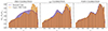 |
Fig. 6. Probability function for the number of voids as a function of redshift for the full-sky sample, illustrating the effects of mock calibration. Left: Void distributions prior to mock calibration. Center: Void distributions following the photometric redshift calibration of the mock galaxies. Right: Void distributions following both photometric redshift and sparseness calibrations. |
We subdivided our void samples into four equispaced redshift bins of Δz = 0.15. For both the total void sample and each redshift bin, we distinguished three different void populations based on their λv values: negative-λv (λv ∈ ( − ∞, −5]), zero-λv (λv ∈ ( − 5, 5]), and positive-λv (λv ∈ (5, ∞)) voids. Figure 7 illustrates that λv is predominantly driven by the mean density inside the voids; however, voids with more positive λv tend to be smaller than those with more negative values, and vice versa. Table 1 summarizes the number of voids for each case considered, showing that the void bins are not equally populated. These specific λv-binning values were chosen to approximately maximize the S/N ratio, with a more refined selection to be explored in future work. Moreover, Fig. 8 compares the probability distributions of void properties – rv,  and λv – for mock and observed voids within each redshift bin.
Number of voids in each sample used.
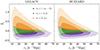 |
Fig. 7. Contours in the |


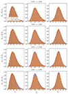 |
Fig. 8. Probability distributions for rv (first column), |

The general agreement between the properties of the simulated and observed void data sets allows us to mitigate potential systematics arising from discrepancies between the two void populations. We highlight that the minor discrepancies observed in the void size functions (left panel of Fig. 8) at both lower and higher redshift bins are likely due to the slight differences in sparseness of the two tracer catalogs, which enhance the sensitivity of voids to this parameter.
3.3. Cross-correlation measurement
Detecting the lensing signal from a single void is challenging (Krause et al. 2013), due to the weak and noisy nature of the signal in current observations. However, measuring a stacked signal from a substantial number of voids can yield a significant detection of the void-lensing cross-correlation. Our approach followed established methods in the literature (e.g., Camacho-Ciurana et al. 2024 and references therein), which are generally consistent. The procedure can be summarized as follows. We initialized two empty 512 × 512 pixel matrices: one to store the final stacked κ values from our CMB lensing map and the other to account for the impact of the CMB mask. The mask applied was the Planck 2018 mask for the observational data, and a corresponding mask covering the populated quarter of the sky for the Buzzard mocks. Pixel weights ranged from 0 (indicating an unobserved pixel) to 1 (indicating a fully observed pixel) and were accumulated progressively. For each void, we extracted a square CMB patch centered at the same sky position as the void center, with a side length equal to five times the angular diameter of the void. This extraction used the gnomonic projection function from healpy (Zonca et al. 2019), the HEALpix Python wrapper. This function identifies the patch by performing an appropriate coordinate rotation and rescales the CMB pixels to match the resolution required by the angular diameter of the void. The same process was applied to the CMB mask. The CMB and mask patches were then added to their respective 512–512 matrices. Once all voids were processed, the stacked CMB patch was normalized by dividing by the weight matrix, yielding the average κ value per pixel, relative to its distance from void centers, while properly accounting for the effects of the CMB mask.
To accurately compare measurements, we corrected for bias introduced by the incomplete observation of the CMB, which caused the mean convergence over the observed area of the sky to deviate from zero. Simply subtracting the mean convergence of the observed region from our stacked patch was insufficient because the voids did not uniformly sample the sky. Some regions were oversampled due to void overlap, which introduced additional complexity to the measurement. We corrected our CMB lensing map by subtracting the bias, which is calculated by averaging all pixels within the circular CMB patches behind the voids with a radius of R = 5rv. Each pixel was weighted according to the number of times it was selected by the overlapping patches.
To compute the cross-correlation, we measured the radial profile of the final stacked patch. We extended our measurement to R = 5rv to capture the influence of the surrounding environment. The radial profile was calculated using 25 bins with a width of dR = 0.2rv, ensuring an optimal balance between noise reduction and profile-fitting accuracy.
3.4. Error estimation and template-fitting analysis
The statistical uncertainty in measuring the void-CMB lensing cross-correlation is dominated by instrumental noise in the Planck CMB temperature measurements. Additional sources of uncertainty include cosmic and sample variances and, to a lesser extent, the error associated with the reconstruction of the convergence maps. The broad sky coverage provided by both Planck (which offers the broadest sky coverage for CMB observations to date) and DESI Legacy observations, combined with the size of the void data set identifiable in the DESI Legacy LRG sample, enabled us to stack our signal from a wide range of independent regions of the Universe and uncorrelated areas of the sky. This resulted in an unprecedented reduction in measurement uncertainty.
To account for these systematic effects, we employed the following strategy for each void sample, based on Vielzeuf et al. (2021). We firstly computed the auto angular auto power spectrum of the anisotropies of the Planck CMB lensing map (Planck Collaboration VIII 2020), Clkk, using the HEALpix function anafast. This quantity is a function of the multipole number l and represents the spherical harmonic decomposition of the CMB lensing convergence field. We then used the HEALpix synfast function to generate 1000 random maps, with nside = 512 and lmax = nside * 3 − 1, based on the measured angular power spectrum. To account for the effects of the CMB mask, we applied a first-order correction to the power spectrum,  , where fsky represents the ratio between the observed and total sky areas. Although fsky varies between 0 and 1, this correction is only reliable when fsky is close to 1. Since fsky ∼ 0.66 in our study, this correction of the power spectrum is adequate. For future studies aiming to constrain cosmological parameters or working with smaller sky regions, a mode-coupling Monte Carlo correction should be considered (see Appendix C of Sailer et al. 2024 for a detailed description of this methodology).
Figure 9 compares the observed PlanckClkk before and after the correction, with the theoretical angular power spectrum derived from the 2018 Planck best-fit cosmology provided by the Planck Collaboration. Finally, monopole and dipole components of the generated maps were removed. Similarly to the procedure applied to the real CMB lensing map, we performed a Gaussian smoothing with a FWHM of 0.5° on each random realization. We then applied Planck CMB lensing mask to the random realization in order to conserve the amount of information contained in every map. Following the procedure outlined in Sect. 3.3, we cross-correlated each randomly generated map with our voids. It was essential to maintain the positions of the void centers to preserve information on void clustering, thereby avoiding overestimation of the errors. To assess the impact of cosmic variance, which arises from working with a single realization of our observable Universe, we performed a jackknife analysis, with NJK = Nv for each bin. This procedure generated a jackknife sample of the same size as the void sample in the considered bin. The standard error associated with each bin was then computed as
 (12)
(12)
 |
Fig. 9. Theoretical (dashed gray line) and observed angular power spectra, shown before (purple line) and after (orange line) the linear correction for the mask effect. The theoretical prediction is derived from the best-fit cosmology of the Planck 2018 results. |
The impact of the jackknife on the error associated with our signal was less than 1.5% for each bin and it was therefore considered negligible. We estimated the elements i, j of the covariance matrix  as
as
 (13)
(13)
where N = 1000 is the size of the random lensing CMB map-voids cross-correlation sample, xik is the measurement of i-th data component of the k-th cross-correlation, and  is the mean measurement of the i-th component. The error bars associated with our measurements were then given by the square root of the diagonal elements of the covariance matrices.
A similar procedure was applied to each CMB mock realization, allowing us to compute the errors associated with the simulated cross-correlations. It is important to note that the contribution from instrumental noise is zero in this case. However, we still accounted for cosmic and sample variance, which contributed non-negligibly to the error budget. The average value of the mock cross-correlation signal was obtained from the mean of the four realizations. The elements of the associated covariance matrix were computed as
 (14)
(14)
where the superscript B refers to “Buzzard”, N is the number of realizations and M denotes the value of the cross-correlation signal. The first term represents the average covariance matrix between the realizations, while the second term accounts for the variance arising from deviations of each simulated signal from the average template.
At this stage, quantified the consistency of our observations with the ΛCDM prediction from the Buzzard mocks. Following the approach outlined in Vielzeuf et al. (2021), we assessed the level of consistency by estimating the best-fitting CMB lensing amplitude parameter, Aκ = κLegacy/κBuzzard along with its corresponding uncertainty, σAκ.
Estimated Aκ parameters for the North and South regions.
The value of Aκ was constrained through a χ2 minimization, with the χ2 statistic given by:
 (15)
(15)
where xi denotes the average CMB lensing signal in a radius bin i and C is the associated covariance matrix. The superscripts L and B denote elements from Legacy Survey and Buzzard mocks, respectively. Each inverse covariance matrix is corrected following the Anderson-Hartlap procedure (Hartlap et al. 2007), by the factor
 (16)
(16)
where Nrandoms = 1000 and Nbins = 25. This correction reduced the covariance values by ∼2.6% which had a small impact on our error measurement. In this statistic, we included the error estimated for the simulated cross-correlations and their relative covariance, rescaled by the factor Ak2. The uncertainty σAκ was determined by identifying the range of Aκ values for which χ2 increases by 1 from its minimum, χmin2. This provided the 1σ confidence interval, assuming that the χ2 distribution was approximately parabolic in the vicinity of the best-fit value.
The S/N associated with our measurement was calculated based on the maximum detected anisotropy as
 (17)
(17)
where Mj and σj denote the measured amplitude of the signal in each bin and its corresponding relative error, respectively.
4. Results and discussion
Following the procedures outlined in the previous sections, we are now able to measure the cross-correlation between the voids identified in the LRGs from the DESI Legacy Survey DR9 and the CMB lensing map from Planck. Furthermore, we estimate the deviation from the ΛCDM predictions based on the analysis of the spectroscopically calibrated LRG population of the Buzzard mocks.
We chose to conduct our analysis by dividing the data set into two distinct regions corresponding to the North and South Galactic Caps, matching each mock realization to the respective data set in order to account for the slight differences in the galaxy catalogs between the two regions. Subsequently, we performed a combined analysis by merging the two regions to account for the full-sky observation. The detailed procedure is outlined in Sect. 3.1.1 and Sect. 3.1.2.
4.1. North and South Galaxy Caps
In our initial analysis, we separately cross-correlated the 78 231 DESI Legacy voids in the North Galaxy Cap and the 62 481 voids in the South Galaxy Cap with the Planck CMB lensing map. To account for the different environments and evolution of our voids, following the procedure illustrated in Nadathur et al. (2017), we further subdivided the data sets according to the λv value of the voids (see Raghunathan et al. 2020; Camacho-Ciurana et al. 2024 and Demirbozan et al. 2024 for previous works exploiting the λv-binning methodology). Specifically, we created three non-equipopulated bins with λv ∈ ( − ∞, −5), λv ∈ [ − 5, 5), and λv ∈ [5, ∞). All observed cross-correlations were then compared with the ΛCDM templates calculated from the Buzzard mocks to estimate the best-fitting CMB lensing amplitude parameter, Aκ, and its corresponding uncertainty, σAκ, providing an estimate of the deviation from the simulated ΛCDM cosmology.
The main results of the analysis of the North and South Galaxy Caps are summarized in Fig. 10. For both the full data set and the three λv bins, we present the observed cross-correlation alongside the simulated ΛCDM signal up to 5rv. The right panel displays the Aκ values for each measurement. Although the simulated signals for the North and South regions appear nearly identical, they exhibit slight differences primarily due to the varying tracer sparseness between the two regions (see Fig. 5) which leads to small differences in the void populations identified. Both regions display similar behavior in the observed cross-correlations, with all measurements consistent with the ΛCDM expectations; fluctuation from Aκ = 1 do not exceed ∼1σ.
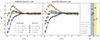 |
Fig. 10. Cross-correlation signals for the voids identified in the North (left) and South (center) regions of DESI Legacy Survey and the corresponding calibrated Buzzard mock realizations. Measurements are shown for the full void samples and the three different λv bins considered. The Aκ values for the various measurements are summarized in the right panel (see Table 2), with yellow and blue vertical bands indicating the 1σ confidence intervals for the full void samples of the North and South regions, respectively. |
Considering the full void sample, we measured Aκ = 1.088 ± 0.081 (S/N = 11.47) for the North region and Aκ = 0.936 ± 0.087 (S/N = 7.83) for the South region. Despite the similarity in the measured signals, the differences in the S/N can be attributed to the varying number of voids and sky coverage in the two regions. As expected, the full sample signals reveal a profile consistent with the projected density profile of the stacked void. Typically, the density contrast profile of voids is negative in their inner part, increasing toward the outer regions in the so-called compensation wall, corresponding to the surrounding walls and filaments and exhibiting positive density contrast values. The cross-correlation profiles similarly show negative convergence in the inner regions, increasing to a positive maximum around r/rv ∼ 1, corresponding to the overdense compensation wall of the stacked void, and then decreasing to zero at larger radii.
When considering the three λv bins, we observe that the void sample is divided into three distinct populations, each exhibiting markedly different lensing characteristics. To understand this behavior, it is important to recall that voids with very negative λv are, by definition, highly underdense, often corresponding to large voids and/or structures likely classified as void-in-voids. Conversely, voids with very positive λv are defined as slightly underdense structures evolving in overdense environments, commonly referred to as void-in-clouds. The distinct nature of these two populations leads to significant differences in their respective lensing signals, resulting in the original cross-correlation being split into three distinct signals. This effect can be exploited to enhance the S/N. For example, in the North region, the negative void sample reaches S/N = 16.06, compared to S/N = 11.47 for the entire void sample in the same Galaxy Cap, resulting in more statistically significant observations. The significance levels of the various measurements, along with the values of the CMB lensing amplitude parameter Aκ and their associated uncertainties, are reported in Table 2, while the number of voids considered in each sample is listed in Table 1.
4.2. Full-sky analysis
As the second step of our analysis, we combined the void samples from the North and South Galaxy Caps to reconstruct the full-sky void catalog, consisting of 140 712 voids. We then compared the observed cross-correlations with the simulated ΛCDM template derived from the 12 North and South Buzzard mock combinations. For details on the full procedure for creating the mock catalogs, refer to Sect. 3.2.2.
Figure 11 presents a detailed view of the stacked CMB patches resulting from the cross-correlation between the full-sky void data set and the CMB lensing map, shown for both the observed data and a single mock realization, as well as for the different λv bins. The first column shows the stacked image for the full void sample, where a distinct negative convergence region is visible at the center of the patches, illustrating the demagnification effect induced by the voids. Furthermore, a positive ring around r ∼ 1rv highlights the magnification effect of the compensation wall. It is evident that the stacked image derived from the DESI Legacy voids appears noisier than that from the simulations, an effect due to residual instrumental noise. The subsequent three columns, from left to right, show the void bins ordered by decreasing λv values from positive to negative. The convergence values of the stacked voids clearly distinguish the different environments in which the void populations evolve.
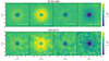 |
Fig. 11. Stacked images of the simulated cross-correlation from the Buzzard mocks (top) and the observed (bottom) cross-correlation between the full-sky void data set from the Legacy Survey and the Planck CMB convergence map. The first column displays the stacked images for the full void population, while the subsequent three columns correspond to void bins categorized by λv, ranging from positive to negative values. Despite the presence of instrumental noise in the observed stacked CMB patches, the images exhibit strong visual agreement between simulations and observations, clearly illustrating the distinct properties of the different void populations analyzed. |
As in the previous analysis, we first cross-correlated the entire void sample and then subdivided the void catalog into three distinct λv bins. The results of the full sky analysis are summarized in Fig. 12, along with the best-fitting CMB lensing amplitude parameters for the signals. We measured Aκ = 1.016 ± 0.054 (S/N = 14.06) for the entire void sample. For the three λv bins, the measured parameters are Aκ = 0.944 ± 0.060 (S/N = 16.94) for the negative λv bin, Aκ = 1.093 ± 0.090 (S/N = 11.33) for the zero λv bin, and Aκ = 0.975 ± 0.060 (S/N = 17.02) for the positive λv bin. These values are also tabulated in Table 3. Once again, all measurements are consistent with the ΛCDM expectations and demonstrate the enhanced S/N achieved by differentiating between the various void populations. This behavior highlights that improving the S/N is not solely dependent on the number of voids but also on the type and quality of the selected void catalog. We note that future analyses could further improve the S/N through optimal fine-tuning of the λv binning.
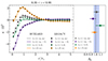 |
Fig. 12. Left: Cross-correlation signals for voids identified in the full-sky DESI Legacy Survey and corresponding calibrated Buzzard mock realizations. Measurements are provided for the full void samples and the three different λv bins considered. Right: Summary of Aκ values for the various measurements (see Table 3). The blue vertical band indicates the 1σ confidence intervals for the full void samples. |
Estimated Aκ parameters for the full-sky sample.
In recent years, Kovács et al. (2022) and Camacho-Ciurana et al. (2024) identified a redshift-dependent tension with the mock-derived ΛCDM prediction in the cross-correlation, with the tension becoming more pronounced at lower redshifts. To address these discrepancies, we extended our analysis by exploiting the large void sample available to conduct a tomographic study of the cross-correlation. We divided the redshift range into four equally spaced bins with Δz = 0.15. Additionally, as in previous studies, we further divided the void sample within each redshift bin into three distinct populations according to their λv values. The number of voids in each bin is reported in Table 1.
The results of the tomographic analysis are shown in Fig. 13, along with a summary plot of the various estimates of the CMB lensing amplitude parameter. For each redshift bin, we measured the following values for the full void samples, from lower to higher redshift, Aκ = 1.025 ± 0.153 (S/N = 5.20), Aκ = 0.993 ± 0.109 (S/N = 7.33), Aκ = 1.041 ± 0.099 (S/N = 7.94), and Aκ = 1.072 ± 0.083 (S/N = 10.34). We observe that for the full void sample, all measurements agree with the mock-derived ΛCDM prediction, with the significance level increasing as the number of voids increases. Furthermore, the cross-correlations exhibit similar amplitudes across the different redshift bins, whereas a stronger signal at higher redshifts would be expected due to the magnification effect of the CMB lensing kernel, which is zero at z = 0 and peaks at z ∼ 1.7 − 1.8. To better understand these behaviors, we separated the void sample based on the λv values of the voids. This procedure allows us to distinguish between different void populations and avoid the signal-flattening effect caused by the combination of voids with varying physical and lensing properties. When analyzing the signals from the negative and positive λv voids separately, both show a coherent evolution, with signal amplitude increasing from low to high redshift.
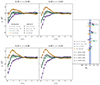 |
Fig. 13. Left: Tomographic cross-correlation signals for the voids identified in the full-sky DESI Legacy Survey and the corresponding calibrated Buzzard mock realizations. The measurements are provided for the full void samples and the three different λv bins, analyzed in four equispaced redshift bins with Δz = 0.15. Right: Summary of Aκ values for the various measurements (see Table 4). The blue vertical band indicates the 1σ confidence intervals for the full void samples from Fig. 12. |
All the measurements are compatible with ΛCDM simulated prediction at the ∼1σ level. The significance levels of the various measurements, along with the Aκ values and their associated uncertainties, are reported in Table 4.
Estimated Aκ parameters for the full-sky tomographic measurements.
We observe that the zero-λv bin, for all redshift bins except the highest, consistently yields an Aκ value slightly above one, at approximately the 1σ level. This bin holds limited cosmological significance due to its intrinsic superposition of various void populations, which results in a cross-correlation amplitude close to zero and a lower significance compared to the other two populations. However, it serves as an important indicator of the alignment between observed and simulated void properties. This void population likely represents voids with an average internal density  . As shown in Fig. 8, these voids are located at the peak of the
  distribution. Consequently, even minor mismatches in
  between observed and simulated void populations (owing to differences in sparseness, error distributions, or other systematics) can cause Aκ values to deviate from one, resulting in apparent discrepancies with the simulated ΛCDM predictions. Despite this trend, it cannot be ruled out that this result is due to random fluctuations. Indeed, considering the excellent overlap between the two void populations, as shown in Fig. 8, and the fact that our measurements aligns with the ΛCDM estimates for the zero-λv bins, we confirm the compatibility between our observed and simulated void populations.
5. Conclusions
In this paper, we present a set of new cross-correlation measurements between cosmic voids and Planck CMB lensing (Planck Collaboration VI 2020; Planck Collaboration VIII 2020). Our work is motivated by the opportunities provided by the new large photometric LRG catalog of the DESI Legacy Survey (Dey et al. 2019), aiming to investigate the tensions with the ΛCDM simulation highlighted by previous studies (Vielzeuf et al. 2021; Hang et al. 2021; Kovács et al. 2022; Camacho-Ciurana et al. 2024).
We compared our observed signals with simulated templates derived from four realizations of the LRG samples from the Buzzard mocks (DeRose et al. 2019), which are designed to mimic the DESI observations and provide realistic DESI-like photometric LRG samples. To address discrepancies between the observed and simulated galaxy catalogs, we corrected our mock realizations by calibrating the photometric redshifts of the mock galaxies, performed using a combination of photometric and spectroscopic redshifts provided by one million DESI spectra (DESI Collaboration 2016a), and matching the sparseness between the observed and simulated galaxy catalogs, as detailed in Sect. 3.1.1 and Sect. 3.1.2.
To create our 3D void samples, we utilized the modified ZOBOV algorithm (Neyrinck 2008), which is integrated into the Revolver void-finding code (Nadathur & Percival 2019). The void identification process and the properties of the void catalogs are summarized in Sect. 3.2. The observed void catalog and the void catalogs from the calibrated mocks show excellent agreement across all considered properties (rv,  and λv), as shown in Fig. 8, which prevents potential tensions between our measurements and the mock-derived ΛCDM predictions that could result from the mismatches between the simulated and observed galaxy sample used for void identification.
Once the void catalogs were produced, we evaluated their κ imprint by cross-correlating with the CMB lensing maps using a stacking methodology. We applied Gaussian smoothing with a FWHM of 0.5° to the CMB lensing maps to mitigate noise and fluctuations at small scales. We then utilized 1000 random CMB realizations to estimate the covariance matrices associated with our measurements. Through a template-fitting process, we assessed the consistency between observed data and the simulated ΛCDM predictions estimating the CMB lensing amplitude parameter Aκ and its uncertainty σAκ.
We independently analyzed the North and South Caps to account for small differences in sparseness levels between the two regions. Subsequently, we merged the two void catalogs to cover the entire sky, modifying our mocks to accordingly reflect the properties of the full-sky observations. The results of the cross-correlation process are reported in Sect. 4. For the full void sample, we measured Aκ = 1.088 ± 0.081 (S/N = 11.47) for the North region, Aκ = 0.936 ± 0.087 (S/N = 7.83) for the South region, and Aκ = 1.016 ± 0.054 (S/N = 14.06) for the full-sky observation. All three measurements are in perfect agreement with the simulated ΛCDM predictions. Furthermore, the full-sky observation provides a new record detection of the CMB lensing signal from voids, with a S/N slightly exceeding those reported in Hang et al. (2021) and Camacho-Ciurana et al. (2024).
To account for the varying environments and evolution of our voids, we subdivided the data sets according to the λv values, creating three non-equipopulated bins: λv ∈ ( − ∞, −5), λv ∈ [ − 5, 5), and λv ∈ [5, ∞), following the procedure illustrated in Nadathur et al. (2017) and Raghunathan et al. (2020). These specific λv-binning values were chosen to approximately maximize the S/N. For the North, South, and full-sky observations, we measured void-CMB lensing cross-correlation signals in perfect agreement with the ΛCDM expectations. The values of the CMB lensing amplitude parameter and corresponding S/N are summarized in Tables. 2 and 3. This analysis underscores the enhanced signal significance obtained by subdividing the void sample into different populations based on their λv values. Specifically, for the full-sky observation, we measured Aκ = 0.944 ± 0.064 (S/N = 16.94) for the void-in-voids population and Aκ = 0.975 ± 0.060 (S/N = 17.02) for the void-in-clouds, which significantly improves the S/N compared to previous observations, despite the smaller number of voids in each sample, and establishes a new record measurement for CMB lensing by voids.
Lastly, we took advantage of the large size of our void catalog to perform a tomographic analysis, subdividing the redshift range into four bins to explore the evolution of the void-CMB lensing signal across different cosmic epochs. Once again, we further subdivided our void samples into three distinct bins based on their λv values, allowing us to disentangle the varying lensing properties of different void populations across the redshift range. As shown in Fig. 13, all observed cross-correlations are consistent with the simulated ΛCDM predictions at ∼1σ level. The corresponding S/N and the measured Aκ values, along with their associated uncertainties, are detailed in Table 4. Once again, this analysis highlights the enhanced power of the signal and the disentangling effect of the λv binning approach, which reveals the evolution of the cross-correlation with redshift driven by the effect of the CMB lensing kernel, otherwise obscured by the overlapping contributions from different void populations to the total signal.
In summary, we presented a set of new cross-correlation measurements between 3D voids and CMB lensing with improved S/N, fully consistent with the ΛCDM predictions from simulations, emphasizing the critical role of systematic management. In particular, we underscore the necessity for mock catalogs used in such analyses to precisely match the observed data in terms of sparseness and redshift error distribution. Even small deviations can lead to void populations with significantly different lensing properties, potentially causing apparent tensions between observations and simulations. This consideration should be prioritized in the development of any future mock catalogs aimed at the cosmological exploitation of voids, ensuring that the systematic alignment between mocks and observations is rigorously maintained to avoid introducing biases in the analysis. Moreover, we demonstrated the importance of the λv binning approach, establishing it as essential for disentangling distinct void populations and improving S/N. This method reveals the redshift evolution of the CMB lensing signal, which would otherwise be obscured by the superposition of different void populations with different physical and lensing properties, allowing for a more precise comparison between observations and mock-derived ΛCDM predictions, thus significantly improving the robustness of the analysis.
In future analyses, further fine-tuning void-in-voids and void-in-clouds populations will be valuable to improve the S/N. This refined approach, combined with the new large spectroscopic data sets from DESI and other next-generation surveys (e.g., Euclid, Vera C. Rubin Observatory, Roman Space Telescope), which will provide high-quality data in the redshift range where the CMB lensing kernel is most sensitive, and with upcoming high-precision CMB observations (e.g., Simons Observatory, CMB-S4), which will greatly reduce noise in convergence maps, is expected to substantially enhance the cosmological constraining power of future measurements of the CMB lensing imprint of voids. These advancements will be critical for future efforts to differentiate between cosmological models and constraining cosmological parameters (see Vielzeuf et al. 2023 for details), offering a new and detailed perspective on cosmic voids and the nature of the Universe.
Data availability
The DESI Legacy Survey DR9 LRG catalog and the Buzzard mocks are available upon request to respectively Rongpu Zhou and Joe DeRose. Planck 2018 CMB lensing data are publicly available on the Planck Legacy Archive at the following link: http://pla.esac.esa.int/pla/#home. Datapoint informations for all the figures of the publication can be found at https://doi.org/10.5281/zenodo.14251132
Acknowledgments
SS would like to thank Chris Blake and Joe DeRose for their efforts in the creation of the Buzzard galaxy mocks and their generous availability, as well as Rongpu Zhou for the creation and publication of the Legacy Survey DR9 sample, which forms the foundation of this work. This material is based upon work supported by the U.S. Department of Energy (DOE), Office of Science, Office of High-Energy Physics, under Contract No. DE–AC02–05CH11231, and by the National Energy Research Scientific Computing Center, a DOE Office of Science User Facility under the same contract. Additional support for DESI was provided by the U.S. National Science Foundation (NSF), Division of Astronomical Sciences under Contract No. AST-0950945 to the NSF’s National Optical-Infrared Astronomy Research Laboratory; the Science and Technology Facilities Council of the United Kingdom; the Gordon and Betty Moore Foundation; the Heising-Simons Foundation; the French Alternative Energies and Atomic Energy Commission (CEA); the National Council of Humanities, Science and Technology of Mexico (CONAHCYT); the Ministry of Science, Innovation and Universities of Spain (MICIU/AEI/10.13039/501100011033), and by the DESI Member Institutions: https://www.desi.lbl.gov/collaborating-institutions. The DESI Legacy Imaging Surveys consist of three individual and complementary projects: the Dark Energy Camera Legacy Survey (DECaLS), the Beijing-Arizona Sky Survey (BASS), and the Mayall z-band Legacy Survey (MzLS). DECaLS, BASS and MzLS together include data obtained, respectively, at the Blanco telescope, Cerro Tololo Inter-American Observatory, NSF’s NOIRLab; the Bok telescope, Steward Observatory, University of Arizona; and the Mayall telescope, Kitt Peak National Observatory, NOIRLab. NOIRLab is operated by the Association of Universities for Research in Astronomy (AURA) under a cooperative agreement with the National Science Foundation. Pipeline processing and analyses of the data were supported by NOIRLab and the Lawrence Berkeley National Laboratory. Legacy Surveys also uses data products from the Near-Earth Object Wide-field Infrared Survey Explorer (NEOWISE), a project of the Jet Propulsion Laboratory/California Institute of Technology, funded by the National Aeronautics and Space Administration. Legacy Surveys was supported by: the Director, Office of Science, Office of High Energy Physics of the U.S. Department of Energy; the National Energy Research Scientific Computing Center, a DOE Office of Science User Facility; the U.S. National Science Foundation, Division of Astronomical Sciences; the National Astronomical Observatories of China, the Chinese Academy of Sciences and the Chinese National Natural Science Foundation. LBNL is managed by the Regents of the University of California under contract to the U.S. Department of Energy. The complete acknowledgments can be found at https://www.legacysurvey.org/. Any opinions, findings, and conclusions or recommendations expressed in this material are those of the author(s) and do not necessarily reflect the views of the U. S. National Science Foundation, the U. S. Department of Energy, or any of the listed funding agencies. The authors are honored to be permitted to conduct scientific research on Iolkam Du’ag (Kitt Peak), a mountain with particular significance to the Tohono O’odham Nation. The Large-Scale Structure (LSS) research group at Konkoly Observatory has been supported by a Lendület excellence grant by the Hungarian Academy of Sciences (MTA). This project has received funding from the European Union’s Horizon Europe research and innovation programme under the Marie Skłodowska-Curie grant agreement number 101130774. Funding for this project was also available in part through the Hungarian Ministry of Innovation and Technology NRDI Office grant OTKA NN147550. This work was supported by the French Space Agency, the Centre National d’Études Spatiales (CNES).
References
- Alonso, D., Hill, J. C., Hložek, R., & Spergel, D. N. 2018, Phys. Rev. D, 97, 063514 [NASA ADS] [CrossRef] [Google Scholar]
- Aubert, M., Cousinou, M.-C., Escoffier, S., et al. 2022, MNRAS, 513, 186 [NASA ADS] [CrossRef] [Google Scholar]
- Baker, T., Clampitt, J., Jain, B., & Trodden, M. 2018, Phys. Rev. D, 98, 023511 [NASA ADS] [CrossRef] [Google Scholar]
- Banerjee, A., & Dalal, N. 2016, JCAP, 2016, 015 [CrossRef] [Google Scholar]
- Barreira, A., Cautun, M., Li, B., Baugh, C. M., & Pascoli, S. 2015, JCAP, 2015, 028 [Google Scholar]
- Bennett, C. L., Larson, D., Weiland, J. L., et al. 2013, ApJS, 208, 20 [Google Scholar]
- Blanchard, A., & Schneider, J. 1987, A&A, 184, 1 [NASA ADS] [Google Scholar]
- Blum, R. D., Burleigh, K., Dey, A., et al. 2016, AAS Meeting Abstr., 228, 317.01 [Google Scholar]
- Bonici, M., Carbone, C., Davini, S., et al. 2023, A&A, 670, A47 [NASA ADS] [CrossRef] [EDP Sciences] [Google Scholar]
- Boschetti, R., Vielzeuf, P., Cousinou, M.-C., Escoffier, S., & Jullo, E. 2024, JCAP, 2024, 067 [CrossRef] [Google Scholar]
- Cai, Y.-C., Neyrinck, M. C., Szapudi, I., Cole, S., & Frenk, C. S. 2014, ApJ, 786, 110 [NASA ADS] [CrossRef] [Google Scholar]
- Cai, Y.-C., Padilla, N., & Li, B. 2015, MNRAS, 451, 1036 [NASA ADS] [CrossRef] [Google Scholar]
- Camacho-Ciurana, G., Lee, P., Arsenov, N., et al. 2024, A&A, 689, A171 [NASA ADS] [CrossRef] [EDP Sciences] [Google Scholar]
- Cautun, M., Paillas, E., Cai, Y.-C., et al. 2018, MNRAS, 476, 3195 [NASA ADS] [CrossRef] [Google Scholar]
- Chan, K. C., Hamaus, N., & Desjacques, V. 2014, Phys. Rev. D, 90, 103521 [NASA ADS] [CrossRef] [Google Scholar]
- Chan, K. C., Hamaus, N., & Biagetti, M. 2019, Phys. Rev. D, 99, 121304 [CrossRef] [Google Scholar]
- Chen, S., DeRose, J., Zhou, R., et al. 2024, arXiv e-prints [arXiv:2407.04795] [Google Scholar]
- Clampitt, J., Cai, Y.-C., & Li, B. 2013, MNRAS, 431, 749 [NASA ADS] [CrossRef] [Google Scholar]
- Clampitt, J., Jain, B., & Sánchez, C. 2016, MNRAS, 456, 4425 [Google Scholar]
- Colberg, J. M., Pearce, F., Foster, C., et al. 2008, MNRAS, 387, 933 [NASA ADS] [CrossRef] [Google Scholar]
- Cole, S., & Efstathiou, G. 1989, MNRAS, 239, 195 [Google Scholar]
- Contarini, S., Ronconi, T., Marulli, F., et al. 2019, MNRAS, 488, 3526 [NASA ADS] [CrossRef] [Google Scholar]
- Contarini, S., Marulli, F., Moscardini, L., et al. 2021, MNRAS, 504, 5021 [NASA ADS] [CrossRef] [Google Scholar]
- Contarini, S., Pisani, A., Hamaus, N., et al. 2023, ApJ, 953, 46 [NASA ADS] [CrossRef] [Google Scholar]
- Correa, C. M., & Paz, D. J. 2022, Bol. Asoc. Argentina Astron. La Plata Argentina, 63, 193 [Google Scholar]
- Correa, C. M., Paz, D. J., Padilla, N. D., et al. 2022, MNRAS, 509, 1871 [Google Scholar]
- Crocce, M., Pueblas, S., & Scoccimarro, R. 2006, MNRAS, 373, 369 [NASA ADS] [CrossRef] [Google Scholar]
- Dawson, K. S., Schlegel, D. J., Ahn, C. P., et al. 2013, AJ, 145, 10 [Google Scholar]
- Dawson, K. S., Kneib, J.-P., Percival, W. J., et al. 2016, AJ, 151, 44 [Google Scholar]
- de Lapparent, V., Geller, M. J., & Huchra, J. P. 1986, ApJ, 302, L1 [Google Scholar]
- Demirbozan, U., Nadathur, S., Ferrero, I., et al. 2024, MNRAS, 534, 2328 [Google Scholar]
- DeRose, J., Wechsler, R. H., Becker, M. R., et al. 2019, ArXiv e-prints [arXiv:1901.02401] [Google Scholar]
- DeRose, J., Becker, M. R., & Wechsler, R. H. 2022, ApJ, 940, 13 [Google Scholar]
- DESI Collaboration (Aghamousa, A., et al.) 2016a, ArXiv e-prints [arXiv:1611.00036] [Google Scholar]
- DESI Collaboration (Aghamousa, A., et al.) 2016b, ArXiv e-prints [arXiv:1611.00037] [Google Scholar]
- Dey, A., Schlegel, D. J., Lang, D., et al. 2019, AJ, 157, 168 [Google Scholar]
- Eisenstein, D. J., Zehavi, I., Hogg, D. W., et al. 2005, ApJ, 633, 560 [Google Scholar]
- Flaugher, B., Diehl, H. T., Honscheid, K., et al. 2015, AJ, 150, 150 [Google Scholar]
- Fraser, T. S., Paillas, E., Percival, W. J., et al. 2024, ArXiv e-prints [arXiv:2407.03221] [Google Scholar]
- Górski, K. M., Hivon, E., Banday, A. J., et al. 2005, ApJ, 622, 759 [Google Scholar]
- Gregory, S. A., & Thompson, L. A. 1978, ApJ, 222, 784 [NASA ADS] [CrossRef] [Google Scholar]
- Hamaus, N., Wandelt, B. D., Sutter, P. M., Lavaux, G., & Warren, M. S. 2014a, Phys. Rev. Lett., 112, 041304 [NASA ADS] [CrossRef] [Google Scholar]
- Hamaus, N., Sutter, P. M., Lavaux, G., & Wandelt, B. D. 2014b, JCAP, 2014, 013 [Google Scholar]
- Hamaus, N., Sutter, P. M., Lavaux, G., & Wandelt, B. D. 2015, JCAP, 2015, 036 [Google Scholar]
- Hamaus, N., Sutter, P. M., & Wandelt, B. D. 2016, IAU Symp., 308, 538 [Google Scholar]
- Hamaus, N., Aubert, M., Pisani, A., et al. 2022, A&A, 658, A20 [NASA ADS] [CrossRef] [EDP Sciences] [Google Scholar]
- Hang, Q., Alam, S., Cai, Y.-C., & Peacock, J. A. 2021, MNRAS, 507, 510 [NASA ADS] [CrossRef] [Google Scholar]
- Hartlap, J., Simon, P., & Schneider, P. 2007, A&A, 464, 399 [NASA ADS] [CrossRef] [EDP Sciences] [Google Scholar]
- Hossen, M. R., Ema, S. A., Bolejko, K., & Lewis, G. F. 2022, MNRAS, 513, 5575 [Google Scholar]
- Hu, W., & Okamoto, T. 2002, ApJ, 574, 566 [CrossRef] [Google Scholar]
- Ilić, S., Langer, M., & Douspis, M. 2013, A&A, 556, A51 [NASA ADS] [CrossRef] [EDP Sciences] [Google Scholar]
- Jennings, E., Li, Y., & Hu, W. 2013, MNRAS, 434, 2167 [CrossRef] [Google Scholar]
- Jõeveer, M., Einasto, J., & Tago, E. 1978, MNRAS, 185, 357 [Google Scholar]
- Kashlinsky, A. 1988, ApJ, 331, L1 [Google Scholar]
- Kirshner, R. P., Oemler, A., Jr, Schechter, P. L., & Shectman, S. A. 1981, ApJ, 248, L57 [NASA ADS] [CrossRef] [Google Scholar]
- Komatsu, E., Smith, K. M., Dunkley, J., et al. 2011, ApJS, 192, 18 [Google Scholar]
- Kovács, A. 2018, MNRAS, 475, 1777 [CrossRef] [Google Scholar]
- Kovács, A., Vielzeuf, P., Ferrero, I., et al. 2022, MNRAS, 515, 4417 [CrossRef] [Google Scholar]
- Krause, E., Chang, T.-C., Doré, O., & Umetsu, K. 2013, ApJ, 762, L20 [NASA ADS] [CrossRef] [Google Scholar]
- Kreisch, C. D., Pisani, A., Carbone, C., et al. 2019, MNRAS, 488, 4413 [NASA ADS] [CrossRef] [Google Scholar]
- Lavaux, G., & Wandelt, B. D. 2010, MNRAS, 403, 1392 [NASA ADS] [CrossRef] [Google Scholar]
- Lavaux, G., & Wandelt, B. D. 2012, ApJ, 754, 109 [NASA ADS] [CrossRef] [Google Scholar]
- Lee, J., & Park, D. 2009, ApJ, 696, L10 [NASA ADS] [CrossRef] [Google Scholar]
- Lewis, A., & Bridle, S. 2002, Phys. Rev. D, 66, 103511 [Google Scholar]
- Li, Y. C., Ma, Y. Z., & Nadathur, S. 2020, ArXiv e-prints [arXiv:2002.01689] [Google Scholar]
- Li, G., Ma, Y.-Z., Tramonte, D., & Li, G.-L. 2024, MNRAS, 527, 2663 [Google Scholar]
- Linder, E. V. 1990, MNRAS, 243, 353 [NASA ADS] [Google Scholar]
- Margon, B. 1999, Philos. Trans. R. Soc. Lond. Ser. A, 357, 93 [Google Scholar]
- Massara, E., Villaescusa-Navarro, F., Viel, M., & Sutter, P. M. 2015, JCAP, 2015, 018 [Google Scholar]
- Massara, E., Percival, W. J., Dalal, N., et al. 2022, MNRAS, 517, 4458 [NASA ADS] [CrossRef] [Google Scholar]
- Mauland, R., Elgarøy, Ø., Mota, D. F., & Winther, H. A. 2023, A&A, 674, A185 [NASA ADS] [CrossRef] [EDP Sciences] [Google Scholar]
- Melchior, P., Sutter, P. M., Sheldon, E. S., Krause, E., & Wandelt, B. D. 2014, MNRAS, 440, 2922 [NASA ADS] [CrossRef] [Google Scholar]
- Moresco, M., Amati, L., Amendola, L., et al. 2022, Liv. Rev. Relativ., 25 [Google Scholar]
- Nadathur, S., & Percival, W. J. 2019, MNRAS, 483, 3472 [NASA ADS] [CrossRef] [Google Scholar]
- Nadathur, S., Hotchkiss, S., & Sarkar, S. 2012, JCAP, 2012, 042 [CrossRef] [Google Scholar]
- Nadathur, S., Hotchkiss, S., & Crittenden, R. 2017, MNRAS, 467, 4067 [Google Scholar]
- Nadathur, S., Carter, P. M., Percival, W. J., Winther, H. A., & Bautista, J. E. 2019, Astrophysics Source Code Library [record ascl:1907.023] [Google Scholar]
- Naidoo, K., Jaber, M., Hellwing, W. A., & Bilicki, M. 2024, Phys. Rev. D, 109, 083511 [Google Scholar]
- Neyrinck, M. C. 2008, MNRAS, 386, 2101 [CrossRef] [Google Scholar]
- Paz, D., Lares, M., Ceccarelli, L., Padilla, N., & Lambas, D. G. 2013, MNRAS, 436, 3480 [NASA ADS] [CrossRef] [Google Scholar]
- Pelliciari, D., Contarini, S., Marulli, F., et al. 2023, MNRAS, 522, 152 [CrossRef] [Google Scholar]
- Perico, E. L. D., Voivodic, R., Lima, M., & Mota, D. F. 2019, A&A, 632, A52 [NASA ADS] [CrossRef] [EDP Sciences] [Google Scholar]
- Perlmutter, S., Aldering, G., Goldhaber, G., et al. 1999, ApJ, 517, 565 [Google Scholar]
- Pisani, A., Sutter, P. M., Hamaus, N., et al. 2015, Phys. Rev. D, 92, 083531 [NASA ADS] [CrossRef] [Google Scholar]
- Pisani, A., Massara, E., Spergel, D. N., et al. 2019, ArXiv e-prints [arXiv:1903.05161] [Google Scholar]
- Planck Collaboration VI. 2020, A&A, 641, A6 [NASA ADS] [CrossRef] [EDP Sciences] [Google Scholar]
- Planck Collaboration VIII. 2020, A&A, 641, A8 [NASA ADS] [CrossRef] [EDP Sciences] [Google Scholar]
- Platen, E., van de Weygaert, R., & Jones, B. J. T. 2007, MNRAS, 380, 551 [NASA ADS] [CrossRef] [Google Scholar]
- Radinović, S., Nadathur, S., Winther, H. A., et al. 2023, A&A, 677, A78 [NASA ADS] [CrossRef] [EDP Sciences] [Google Scholar]
- Radinović, S., Winther, H. A., Nadathur, S., et al. 2024, A&A, 691, A39 [NASA ADS] [CrossRef] [EDP Sciences] [Google Scholar]
- Raghunathan, S., Nadathur, S., Sherwin, B. D., & Whitehorn, N. 2020, ApJ, 890, 168 [NASA ADS] [CrossRef] [Google Scholar]
- Rezaei, Z. 2020, ApJ, 902, 102 [Google Scholar]
- Riess, A. G., Filippenko, A. V., Challis, P., et al. 1998, AJ, 116, 1009 [Google Scholar]
- Ronconi, T., Contarini, S., Marulli, F., Baldi, M., & Moscardini, L. 2019, MNRAS, 488, 5075 [NASA ADS] [CrossRef] [Google Scholar]
- Ryden, B. S. 1995, ApJ, 452, 25 [NASA ADS] [CrossRef] [Google Scholar]
- Sachs, R. K., & Wolfe, A. M. 1967, ApJ, 147, 73 [NASA ADS] [CrossRef] [Google Scholar]
- Sailer, N., Kim, J., Ferraro, S., et al. 2024, ArXiv e-prints [arXiv:2407.04607] [Google Scholar]
- Sánchez, C., Clampitt, J., Kovacs, A., et al. 2017, MNRAS, 465, 746 [CrossRef] [Google Scholar]
- Sasaki, M. 1989, MNRAS, 240, 415 [Google Scholar]
- Schlegel, D., Dey, A., Herrera, D., et al. 2021, AAS Meeting Abstr., 237, 235.03 [Google Scholar]
- Schmidt, B. P., Suntzeff, N. B., Phillips, M. M., et al. 1998, ApJ, 507, 46 [NASA ADS] [CrossRef] [Google Scholar]
- Schuster, N., Hamaus, N., Pisani, A., et al. 2019, JCAP, 2019, 055 [Google Scholar]
- Schuster, N., Hamaus, N., Dolag, K., & Weller, J. 2023, JCAP, 2023, 031 [CrossRef] [Google Scholar]
- Schuster, N., Hamaus, N., Dolag, K., & Weller, J. 2024, JCAP, 2024, 065 [Google Scholar]
- Sheth, R. K., & van de Weygaert, R. 2004, MNRAS, 350, 517 [NASA ADS] [CrossRef] [Google Scholar]
- Silva, D. R., Blum, R. D., Allen, L., et al. 2016, AAS Meeting Abstr., 228, 317.02 [Google Scholar]
- Song, Y., Xiong, Q., Gong, Y., et al. 2024, ApJ, 976, 244 [Google Scholar]
- Spolyar, D., Sahlén, M., & Silk, J. 2013, Phys. Rev. Lett., 111, 241103 [NASA ADS] [CrossRef] [Google Scholar]
- Springel, V. 2005, MNRAS, 364, 1105 [Google Scholar]
- Sunyaev, R. A., & Zeldovich, Y. B. 1970, Ap&SS, 7, 3 [NASA ADS] [Google Scholar]
- Sutter, P. M., Lavaux, G., Wandelt, B. D., & Weinberg, D. H. 2012, ApJ, 761, 187 [NASA ADS] [CrossRef] [Google Scholar]
- Sutter, P. M., Pisani, A., Wandelt, B. D., & Weinberg, D. H. 2014, MNRAS, 443, 2983 [NASA ADS] [CrossRef] [Google Scholar]
- The Dark Energy Survey Collaboration 2005, ArXiv e-prints [arXiv:astro-ph/0510346] [Google Scholar]
- Thiele, L., Massara, E., Pisani, A., et al. 2024, ApJ, 969, 89 [NASA ADS] [CrossRef] [Google Scholar]
- Tomita, K., & Watanabe, K. 1989, Prog. Theor. Phys., 82, 563 [Google Scholar]
- Verza, G., Carbone, C., Pisani, A., Porciani, C., & Matarrese, S. 2024, JCAP, 2024, 079 [Google Scholar]
- Vielzeuf, P., Kovács, A., Demirbozan, U., et al. 2021, MNRAS, 500, 464 [Google Scholar]
- Vielzeuf, P., Calabrese, M., Carbone, C., Fabbian, G., & Baccigalupi, C. 2023, JCAP, 2023, 010 [CrossRef] [Google Scholar]
- Wechsler, R. H., DeRose, J., Busha, M. T., et al. 2022, ApJ, 931, 145 [NASA ADS] [CrossRef] [Google Scholar]
- Wilson, C., & Bean, R. 2023, Phys. Rev. D, 107, 124008 [Google Scholar]
- Woodfinden, A., Nadathur, S., Percival, W. J., et al. 2022, MNRAS, 516, 4307 [NASA ADS] [CrossRef] [Google Scholar]
- Woodfinden, A., Percival, W. J., Nadathur, S., et al. 2023, MNRAS, 523, 6360 [NASA ADS] [CrossRef] [Google Scholar]
- Wright, E. L., Eisenhardt, P. R. M., Mainzer, A. K., et al. 2010, AJ, 140, 1868 [Google Scholar]
- York, D. G., Adelman, J., Anderson, J. E., Jr, et al. 2000, AJ, 120, 1579 [Google Scholar]
- Zhou, R., Dey, B., Newman, J. A., et al. 2023, AJ, 165, 58 [NASA ADS] [CrossRef] [Google Scholar]
- Zivick, P., & Sutter, P. M. 2016, IAU Symp., 308, 589 [Google Scholar]
- Zivick, P., Sutter, P. M., Wandelt, B. D., Li, B., & Lam, T. Y. 2015, MNRAS, 451, 4215 [NASA ADS] [CrossRef] [Google Scholar]
- Zonca, A., Singer, L., Lenz, D., et al. 2019, J. Open Source Softw., 4, 1298 [Google Scholar]
- Zou, H., Zhou, X., Fan, X., et al. 2017, PASP, 129, 064101 [CrossRef] [Google Scholar]
All Tables
All Figures
|
Fig. 1. Footprints of the MzLS+BASS, DECaLS, and DES surveys that compose the DESI Legacy Survey, covering a total observed sky area of 19 573 deg2. |
| In the text | |
|
Fig. 2. Planck CMB lensing map, smoothed with a Gaussian filter of FWHM = 0.5°. The DESI Legacy Survey footprint is overlaid, indicating the region where voids are identified and cross-correlations are performed. The footprint is divided into North and South regions, corresponding to the North and South Galactic Caps. CMB regions with negative and positive convergence values are represented by the blue and red ranges of the color palette, respectively. |
| In the text | |
|
Fig. 3. Redshift error distributions for the observed and one simulated LRG data sets, shown in orange and purple, respectively, at the 68.27th, 95.45th, and 99.73th percentiles. Darker shades represent smaller percentile ranges. The two distributions exhibit distinct trends and deviations from zero, which must be corrected to ensure proper matching between observations and mocks. |
| In the text | |
|
Fig. 4. Redshift evolution of the MGS observed in the Legacy Survey (orange dots) compared with the MGSs of the four Buzzard mock realizations before (purple lines) and after (green lines) photometric redshift correction. The shape change after correction, now matching the MGS trend of the Legacy Survey galaxy sample, strongly indicates the accuracy of the redshift calibration procedure. |
| In the text | |
|
Fig. 5. Redshift evolution of the MGS observed in the Legacy Survey, measured in the North (orange dots) and South (white dots) regions. The observed MGS values are compared with those from the four redshift-calibrated Buzzard mock realizations before (purple lines) and then after sparseness correction, performed independently to match the North (green lines) and South (gray lines) regions. An almost complete match is observed between the observations and simulations, with only minor differences at z ∼ 0.4 and z > 0.8, where the mocks appear more sparse than the observations, making subsampling infeasible. |
| In the text | |
|
Fig. 6. Probability function for the number of voids as a function of redshift for the full-sky sample, illustrating the effects of mock calibration. Left: Void distributions prior to mock calibration. Center: Void distributions following the photometric redshift calibration of the mock galaxies. Right: Void distributions following both photometric redshift and sparseness calibrations. |
| In the text | |
|
Fig. 7. Contours in the |
| In the text | |
|
Fig. 8. Probability distributions for rv (first column), |
| In the text | |
|
Fig. 9. Theoretical (dashed gray line) and observed angular power spectra, shown before (purple line) and after (orange line) the linear correction for the mask effect. The theoretical prediction is derived from the best-fit cosmology of the Planck 2018 results. |
| In the text | |
|
Fig. 10. Cross-correlation signals for the voids identified in the North (left) and South (center) regions of DESI Legacy Survey and the corresponding calibrated Buzzard mock realizations. Measurements are shown for the full void samples and the three different λv bins considered. The Aκ values for the various measurements are summarized in the right panel (see Table 2), with yellow and blue vertical bands indicating the 1σ confidence intervals for the full void samples of the North and South regions, respectively. |
| In the text | |
|
Fig. 11. Stacked images of the simulated cross-correlation from the Buzzard mocks (top) and the observed (bottom) cross-correlation between the full-sky void data set from the Legacy Survey and the Planck CMB convergence map. The first column displays the stacked images for the full void population, while the subsequent three columns correspond to void bins categorized by λv, ranging from positive to negative values. Despite the presence of instrumental noise in the observed stacked CMB patches, the images exhibit strong visual agreement between simulations and observations, clearly illustrating the distinct properties of the different void populations analyzed. |
| In the text | |
|
Fig. 12. Left: Cross-correlation signals for voids identified in the full-sky DESI Legacy Survey and corresponding calibrated Buzzard mock realizations. Measurements are provided for the full void samples and the three different λv bins considered. Right: Summary of Aκ values for the various measurements (see Table 3). The blue vertical band indicates the 1σ confidence intervals for the full void samples. |
| In the text | |
|
Fig. 13. Left: Tomographic cross-correlation signals for the voids identified in the full-sky DESI Legacy Survey and the corresponding calibrated Buzzard mock realizations. The measurements are provided for the full void samples and the three different λv bins, analyzed in four equispaced redshift bins with Δz = 0.15. Right: Summary of Aκ values for the various measurements (see Table 4). The blue vertical band indicates the 1σ confidence intervals for the full void samples from Fig. 12. |
| In the text | |
Current usage metrics show cumulative count of Article Views (full-text article views including HTML views, PDF and ePub downloads, according to the available data) and Abstracts Views on Vision4Press platform.
Data correspond to usage on the plateform after 2015. The current usage metrics is available 48-96 hours after online publication and is updated daily on week days.
Initial download of the metrics may take a while.