| Issue |
A&A
Volume 691, November 2024
|
|
|---|---|---|
| Article Number | A39 | |
| Number of page(s) | 19 | |
| Section | Cosmology (including clusters of galaxies) | |
| DOI | https://doi.org/10.1051/0004-6361/202451358 | |
| Published online | 29 October 2024 | |
Alcock–Paczyński effect on void-finding
Implications for void-galaxy cross-correlation modelling
1
Institute of Theoretical Astrophysics, University of Oslo,
PO Box 1029, Blindern
0315,
Oslo,
Norway
2
Institute of Space Sciences (ICE, CSIC), Campus UAB, Carrer de Can Magrans, s/n,
08193
Barcelona,
Spain
3
Institute of Cosmology and Gravitation, University of Portsmouth,
Burnaby Road,
Portsmouth
PO1 3FX,
UK
4
Waterloo centre for Astrophysics, University of Waterloo,
200 University Ave W,
Waterloo,
ON
N2L 3G1,
Canada
5
Department of Physics and Astronomy, University of Waterloo,
200 University Ave W,
Waterloo,
ON
N2L 3G1,
Canada
6
Perimeter Institute for Theoretical Physics,
31 Caroline St. North,
Waterloo,
ON
N2L 2Y5,
Canada
★ Corresponding author; This email address is being protected from spambots. You need JavaScript enabled to view it.
Received:
3
July
2024
Accepted:
23
September
2024
Abstract
Under the assumption of statistical isotropy, and in the absence of directional selection effects, a stack of voids is expected to be spherically symmetric, which makes it an excellent object to use for an Alcock–Paczyński (AP) test. This test is commonly carried out using the void-galaxy cross-correlation function (CCF), which has emerged as a competitive probe, especially in combination with the galaxy-galaxy auto-correlation function. Current studies of the AP effect around voids assume that void-centre positions are influenced by the choice of fiducial cosmology in the same way as galaxy positions. We show that this assumption, though prevalent in the literature, is complicated by the response of void-finding algorithms to shifts in tracer positions. Using stretched simulation boxes to emulate the AP effect, we investigate how the void-galaxy CCF changes due to its presence, revealing an additional effect imprinted in the CCF that must be accounted for. The effect originates from the response of void finders to the distorted tracer field – which leads to reduction of the amplitude of the AP signal in the CCF – and thus depends on the specific void-finding algorithm used. We present results for four different void-finding packages, namely REVOLVER, VIDE, voxel, and the spherical void finder in the Pylians3 library, demonstrating how incorrect treatment of the AP effect results in biases in the recovered parameters, regardless of the technique used. Finally, we propose a method to alleviate this issue without resorting to complex and finder-specific modelling of the void-finder response to AP.
Key words: cosmology: theory / large-scale structure of Universe
© The Authors 2024
 Open Access article, published by EDP Sciences, under the terms of the Creative Commons Attribution License (https://creativecommons.org/licenses/by/4.0), which permits unrestricted use, distribution, and reproduction in any medium, provided the original work is properly cited.
This article is published in open access under the Subscribe to Open model. This email address is being protected from spambots. You need JavaScript enabled to view it. to support open access publication.
1 Introduction
The large-scale structure of the Universe contains a lot of information about its expansion history, as well as the growth of structure within it. The standard way to extract this information is to compute the galaxy-galaxy two-point statistics (either the correlation function or its Fourier equivalent, the power spectrum): the isolated baryon acoustic oscillation (BAO) feature measurable in these statistics can be used as a standard ruler to extract information on the background cosmology (e.g. Alam et al. 2015, 2021), or the full shape of the two-point clustering can be used to extract perturbation information, which includes the signatures of galaxy velocities that give rise to redshift-space distortions (RSD; Kaiser 1987). Over the last decade, cosmic voids, and in particular the use of the void-galaxy cross-correlation function (CCF), have become a powerful probe that is complementary to these standard analysis techniques. To study the void-galaxy CCF, we must locate the voids – regions of low local galaxy density – within a galaxy sample and cross-correlate the positions of void centres with the galaxy positions. The advantage of the void-galaxy CCF comes from two facts: first, in absence of any directional distortions or selection effects, and for a large enough sample of voids, the CCF should be spherically symmetric and is therefore a good candidate to perform the Alcock–Paczyński (AP) test on (Alcock & Paczynski 1979; Lavaux & Wandelt 2012); second, the dominant source of such directional distortions arises from the coherent outflow velocity from the centres of voids towards over-densities at the boundary, but this can be modelled relatively accurately, thus enabling the AP test. A simple model for the outflow velocity based on linear perturbation theory (Hamaus et al. 2014; Cai et al. 2016; Nadathur & Percival 2019; Paillas et al. 2021; Massara et al. 2022; Schuster et al. 2023) has been shown to work sufficiently well for the level of statistical precision afforded by data from Stage-III galaxy surveys such as the Baryon Oscillation Spectroscopic Survey (BOSS).
The void-galaxy CCF has been measured in data from the Sloan Digital Sky Survey (SDSS) (York et al. 2000; Eisenstein et al. 2011; Blanton et al. 2017) in several studies (e.g. Paz et al. 2013; Hamaus et al. 2016; Hawken et al. 2017; Nadathur et al. 2019b; Achitouv 2019; Hawken et al. 2020; Aubert et al. 2022; Woodfinden et al. 2022), and has been used to place tight constraints on the parameter combination DM H(z)/c via the AP test, where DM(z) is the angular diameter distance and H(z) is the Hubble rate at redshift z, as well as on the growth rate of structure fσ8. Various other observables related to voids have also been considered, such as the void size function (e.g. Pisani et al. 2015; Nadathur 2016; Correa et al. 2019; Contarini et al. 2022), gravitational lensing by voids (e.g. Sánchez et al. 2017; Raghunathan et al. 2020; Bonici et al. 2023), secondary cosmic microwave background (CMB) anisotropies (e.g. Granett et al. 2008; Nadathur & Crittenden 2016; Alonso et al. 2018; Kovács et al. 2019), and void clustering (e.g. Chan et al. 2014; Kitaura et al. 2016; Zhao et al. 2022).
In any void study, a choice must first be made as to what constitutes a void; there is no agreed canonical definition, and many different void-finding algorithms exist, each giving rise to a different final population (see e.g. Colberg et al. 2008, for a comparison of some algorithms, although many new ones have since been published). As voids are extended objects and are not spherical in general, for the same physical void, the location of the void centre may also be defined in multiple ways (Nadathur & Hotchkiss 2015). These are not necessarily problems for observational constraints as long as the void population thus defined corresponds to under-dense regions without unwanted selection biases, and the outflow velocity around the chosen void centre location can be accurately modelled.
Another consideration is whether to identify voids by applying the void-finding algorithm directly on the observed redshift-space galaxy positions or on a galaxy catalogue with large-scale RSD removed (Nadathur et al. 2019b). The first option is simpler to implement, but leads to a catalogue with selection effects dependent on the void orientation (Nadathur et al. 2019a; Correa et al. 2022; Radinović et al. 2023) and with additional imprints of RSD on the void centre positions, necessitating additional corrections to the modelling (see Nadathur et al. 2020, for an extended discussion).
To be able to locate voids in observational data, we need to assume a fiducial cosmology to first convert observed galaxy redshift and sky angles to distances. If the chosen fiducial cosmology does not match the true cosmology of the Universe, the resulting 3D map of galaxy positions is affected by AP distortions. If they can be correctly modelled, they are a source of information on the background cosmology via the AP test. For the galaxy-galaxy two-point function, modelling the effect of AP distortions is straightforward: as each galaxy position is determined from its measured redshift in the same way, their positions transform under the same relations and the AP distortion in the correlation function can be modelled as a simple rescaling of the pair-separation distances along and perpendicular to the line of sight by the so-called AP scaling parameters, which relate DM and H in the true cosmology to their values in the assumed fiducial one.
However, for voids, the situation is more complex, as there is no physical object associated with the centre of a void whose redshift can be directly measured. Instead, the void position is determined from the application of an algorithm on the catalogue of very many galaxies, the positions of each of which already contain AP distortions. To simplify the modelling of the void-galaxy CCF, it has thus far been implicitly assumed that the resultant void-centre position transforms depending on the choice of fiducial cosmology in the same way as galaxy positions do, and thus that void-galaxy pair-separation distances can be rescaled using the scaling parameters as is the case for galaxy-galaxy separations. In this paper, we examine the validity of this assumption and show that in general it does not hold, as the two operations of ‘AP distortion’ and ‘void-finding’ do not commute. The validity of the approximation in theoretical models of the void-galaxy CCF derived under this assumption will depend on the specific void-finding algorithm in question and the difference between the true cosmological background and the assumed fiducial model (specifically on the degree of anisotropy introduced by the AP distortion). The aim of this paper is to bring attention to this effect, quantify its size for a few common void-finding algorithms, and propose ways of mitigating this issue. We note that accounting for this effect is only important when the effect of the AP distortion is modelled analytically; it is already appropriately included in simulation-based modelling approaches (e.g. Paillas et al. 2024; Fraser et al. 2024).
The layout of this paper is as follows: in Sect. 2 we give an overview of the distances in cosmology including the AP effect and RSD. In Sect. 3, we review the theoretical model for the void-galaxy CCF. In Sect. 4, we outline the methods we used and the different void-finder algorithms. In Sect. 5, we show our results for how the different void-finders respond to AP distortions before concluding in Sect. 6.
2 Distances in cosmology
2.1 Alcock–Paczyński distortions
Instead of physical distances, the positions of observed celestial objects are given by angles in the sky, θ and ϕ, as well as their measured redshift z. The comoving distance to the object is given by
![Mathematical equation: $\[\chi(z)=\int_0^z \frac{c \mathrm{~d} z}{H(z)}.\]$](/articles/aa/full_html/2024/11/aa51358-24/aa51358-24-eq1.png) (1)
(1)
As we see, the transformation to physical distances requires us to choose H(z), that is to assume a fiducial cosmology. If this assumed cosmology is different from the true one, the inferred positions will be wrong, leading to Alcock–Paczyński (AP) distortions (Alcock & Paczynski 1979).
For pairs of objects which both have measured redshifts, this logic extends to the distances between them. Let us define the separation vector r of such a pair of objects, which we can decompose along and perpendicular to the line of sight such that
![Mathematical equation: $\[r=\sqrt{r_{\|}^2+r_{\perp}^2}.\]$](/articles/aa/full_html/2024/11/aa51358-24/aa51358-24-eq2.png) (2)
(2)
At redshift z, distances perpendicular to the line of sight (LoS) are directly related to the comoving angular diameter distance DM(z), while distances along the LoS are related to the Hubble distance DH(z) = c/H(z). Thus, when the assumed (fiducial) cosmology is slightly different from the truth, these distances are rescaled by the factors
![Mathematical equation: $\[q_{\|} \equiv \frac{D_{\mathrm{H}}^{\text {true }}(z)}{D_{\mathrm{H}}^{\text {fid }}(z)},\]$](/articles/aa/full_html/2024/11/aa51358-24/aa51358-24-eq3.png) (3)
(3)
![Mathematical equation: $\[q_{\perp} \equiv \frac{D_{\mathrm{M}}^{\mathrm{true}}(z)}{D_{\mathrm{M}}^{\mathrm{fid}}(z)},\]$](/articles/aa/full_html/2024/11/aa51358-24/aa51358-24-eq4.png) (4)
(4)
Here, and throughout the paper, we use the superscript true to denote quantities and distances computed in the true cosmology, and superscript fid for quantities and distances in the fiducial one.
Now we can write the relation between true distances and the ones inferred using the fiducial cosmology as
![Mathematical equation: $\[r_{\|}^{\text {true }}=q_{\|} r_{\|}^{\text {fid }},\]$](/articles/aa/full_html/2024/11/aa51358-24/aa51358-24-eq5.png) (5)
(5)
![Mathematical equation: $\[r_{\perp}^{\text {true }}=q_{\perp} r_{\perp}^{\text {fid }}.\]$](/articles/aa/full_html/2024/11/aa51358-24/aa51358-24-eq6.png) (6)
(6)
In order to account for the AP effect in modelling the autocorrelation of galaxies (or the power spectrum equivalent in Fourier space), it is therefore sufficient to rescale the separation vectors along and across the line of sight by q‖ and q⊥, and this approach is extensively used in galaxy survey analyses. The q‖ and q⊥ parameters can be expressed through an isotropic volumetric distortion parameter
![Mathematical equation: $\[q=q_{\perp}^{2 / 3} q_{\|}^{1 / 3},\]$](/articles/aa/full_html/2024/11/aa51358-24/aa51358-24-eq7.png) (7)
(7)
which can be determined through measurement of a feature with an externally known and well-defined physical scale, such as the BAO peak, and the combination
![Mathematical equation: $\[\epsilon=\frac{q_{\perp}}{q_{\|}},\]$](/articles/aa/full_html/2024/11/aa51358-24/aa51358-24-eq8.png) (8)
(8)
which quantifies the anisotropy introduced due to the AP effect.
Models of the void-galaxy CCF (Paz et al. 2013; Hamaus et al. 2016; Nadathur & Percival 2019; Hamaus et al. 2022) have thus far assumed that the distortion of the CCF can be captured using the (q‖, q⊥) or (q, ε) parameter pairs1. This is equivalent to assuming that the application of the void-finding algorithm to a set of galaxy positions with or without AP distortions would return exactly the same population of voids, but with the void centre positions shifted by exactly the same amounts as predicted by the AP effect, that is, Eqs. (5) and (6). Since voids positions are inferred from the large-scale galaxy distribution, rather than being computed from a single measured redshift via the application of Eq. (1), this is a non-trivial assumption whose validity remains to be confirmed. In addition to this, there is also the possibility that voids may not form a statistically isotropic population if the chosen fiducial cosmology is far from the truth: that is, void-finding algorithms which have no preferred orientation when applied to a galaxy distribution with no AP distortion, may return samples of voids preferentially aligned either along, or perpendicular to, the LoS when (q‖, q⊥) ≠ (1, 1).
2.2 Redshift-space distortions
Peculiar velocities of objects interfere with redshift determination by inducing RSD (Kaiser 1987) along the LoS. Because these velocities contain a wealth of information about the growth of structure, accurately modelling RSD can help us constrain the way cosmic structures evolve over time.
For two objects with a LoS component of the pairwise peculiar velocity v‖, we can relate the real-space separation r to the distorted separation in redshift space, s, by:
![Mathematical equation: $\[s_{\|}=r_{\|}+\frac{v_{\|}}{a H},\]$](/articles/aa/full_html/2024/11/aa51358-24/aa51358-24-eq9.png) (9)
(9)
![Mathematical equation: $\[s_{\perp}=r_{\perp},\]$](/articles/aa/full_html/2024/11/aa51358-24/aa51358-24-eq10.png) (10)
(10)
where we explicitly see that the distortion only occurs along the LoS, while separation distances perpendicular to the LoS remain unchanged.
When applying this modelling to the void-galaxy CCF, it is typical to assume that the void positions themselves do not transform under the shift from real to redshift space, so that v‖ refers to the peculiar velocities of the galaxies alone. However, as there is no physical object at the void centre whose redshift is measured, the assigned location of the void centre is merely a convention. In practice all studies define the void positions only once, using either the observed galaxy positions in redshift space, or the galaxy positions with large-scale RSD removed, but not both2. Thus the void positions are invariant under the mapping of galaxies from real to redshift space by construction and any actual motion of void centres is irrelevant – see Massara et al. (2022) for further discussion.
We note the asymmetry between the conventional treatment of AP and RSD for voids here. The situations are analogous because in both cases void positions are not obtained from an observed redshift of the void, but indirectly determined from the galaxy field – which may or may not contain LoS distortions – and then held fixed and not further transformed. However, while the conventional treatment for RSD (correctly) includes velocity contributions to the inferred positions of galaxies but not to the fixed void positions, the conventional treatment for AP distortions in Eqs. (5) and (6) implicitly assumes that the void positions transform in the same way as galaxies.
For simplicity, a schematic overview of the relationship between distances in real and redshift space, as well as the relationship between them in the true and fiducial cosmologies, is given in Fig. 1.
3 Theory
3.1 The Alcock–Paczyński effect in the void-galaxy cross-correlation function
Both of the distortion effects described above leave distinct signatures in the void-galaxy CCF ξ(r), which describes the excess probability over random of finding a galaxy at some distance r from the void. As the signatures that these two effects leave in the CCF are different, we can use it to disentangle and constrain them individually.
In the literature, the AP treatment for the void-galaxy CCF is based on the one used in galaxy clustering, and uses the equation
![Mathematical equation: $\[\xi_{\text {fid }}\left(\mathbf{r}^{\text {fid }}\right)=\xi_{\text {true }}\left(\mathbf{r}^{\text {true }}\right),\]$](/articles/aa/full_html/2024/11/aa51358-24/aa51358-24-eq11.png) (11)
(11)
which relates the CCF in the true and fiducial cosmologies. Equation (11) relies on the implicit assumption that voids in the AP-distorted galaxy field are simply shifted versions of the voids in the undistorted field, and that the shifts in their positions are the same as the shifts that would be incurred by a galaxy located at those original positions. However, the knowledge that recovered void positions depend on the detailed positions of many galaxies, and that they vary strongly with the details of the specific void-finding algorithm used, already suggests that this might not be the case. AP shifts in the tracer field will be translated into shifts in void positions which are not immediately obvious or trivial.
In order to demonstrate this, we construct an idealised test scenario using simulated data (the details of the simulations and void algorithms are described in detail in Sect. 4). Given a catalogue of simulated (halo) tracers in real space, we shift their positions by stretching their coordinates parallel and perpendicular to an arbitrary LoS direction according to Eqs. (5) and (6) in order to mimic an AP distortion, with stretch factors q‖ and q⊥ chosen for demonstration purposes in order to maintain the volume but introduce a substantial anisotropy, q = 1 and ε = 1.053. We create one void catalogue from the application of the void-finding algorithm to these shifted tracers, and a second one from applying the algorithm to the original tracer positions, but then shifting the obtained void positions by q‖ and q⊥ according to Eqs. (5) and (6). When cross-correlating with the AP-distorted tracer positions, using the first void catalogue provides a realistic representation of the CCF ξfid(rfid) that could be measured in actual survey data, while using the second gives the idealised CCF when void positions are shifted like those of the halo tracers. If the assumption underlying void-galaxy CCF models in the literature is correct, these two approaches should give the same result.
Figure 2 shows the quadrupole moment of the CCF obtained in these two cases (green and yellow lines respectively). For comparison, we also show the CCF quadrupole for the case with no AP shifts to either tracer or void positions (red). Decomposition of the CCF into Legendre multipoles is standard practice, and the quadrupole moment can effectively summarise the anisotropy of the CCF – since q = 1 in this demonstration, the monopole of the CCF will be the same in each of the three cases. Unsurprisingly, the quadrupole in the true cosmology (with neither the AP effect nor RSD) is consistent with zero, telling us that the CCF is spherically symmetric, while the other two show significant deviations from spherical symmetry due to the AP effect. It is clear that there is a large difference between the realistic case, where voids were found in the distorted tracer field, and the assumed case where the AP effect affects both tracers and voids in the same way.
As we will discuss in detail below, this difference in the CCF between the two cases has important consequences for the theory models of the CCF that have been developed so far, leading to systematic modelling errors in scenarios with an anisotropic AP distortion (ε ≠ 1) between the true and fiducial cosmologies. Correcting the models for this requires accounting for the effect of AP shifts on the void-finding algorithm itself. However, since this will be different for different void-finding algorithms, we will forgo trying to analytically describe it and in the following instead attempt to circumvent the problem.
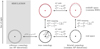 |
Fig. 1 Overview of the different coordinates in use and the transformations between them. Bottom centre is a schematic representation of a void in real space in the true cosmology. The overall shape of the void is spherical, as expected from statistical isotropy. In the top panel (red), we apply a redshift-space distortion, which elongates the void along the line of sight. The right-hand side shows what happens when the wrong cosmology is assumed in the analysis, while the left-hand side shows voids from a simulation used to obtain templates, which are spherically symmetric but whose sizes may vary in simulations with different cosmologies. |
3.2 Modelling redshift-space distortions
The second component of models for the CCF between voids and galaxy (or halo) tracers3 is accounting for RSD due to the outflow velocities of the tracers around voids. Conservation of void-tracer pairs gives the relationship
![Mathematical equation: $\[1+\xi^{\mathrm{s}}(\mathbf{s})=\int\left[1+\xi^{\mathrm{r}}(\mathbf{r})\right] P\left(v_{\|}, \mathbf{r}\right) \mathrm{d} \mathrm{v}_{\|}\]$](/articles/aa/full_html/2024/11/aa51358-24/aa51358-24-eq12.png) (12)
(12)
between the real-space CCF ξr and the redshift-space one ξs. This is realized through a convolution of ξr with a probability distribution P(v‖, r) that describes the distribution of the LoS components of tracer peculiar velocities v‖ (as mentioned earlier in Sect. 2.2, this does not include a contribution from the ‘motion’ of voids).
Following the notation of Radinović et al. (2023), we include an extra leading superscript to denote whether the CCF is computed using the positions of voids found in the redshift-space (s) or real-space (r) tracer fields: for example, for the CCF with redshift-space tracer positions, these two scenarios would be denoted by ξss and ξrs, respectively, and similarly for the realspace CCF. As has already been noted in many studies (e.g. Chuang et al. 2017; Nadathur et al. 2019a; Correa et al. 2022), performing void-finding on the redshift-space tracer field introduces an additional source of anisotropies, so these CCFs are in general not the same, for example ξss ≠ ξrs. Also, since void numbers are in general not conserved through the application of the void-finding algorithm on different spaces, Eq. (12) can only be used to relate CCFs computed with the same void catalogue on either side of the equation, that is, ξss and ξsr or ξrs and ξrr, but not ξss and ξrr. For the main results in this paper we follow the methodology of previous studies (Nadathur & Percival 2019; Nadathur et al. 2019b; Woodfinden et al. 2022; Radinović et al. 2023) and use ξrs and ξrr obtained from voids identified in the real space tracer field without RSD, but in Appendix B we demonstrate that the conclusions regarding the importance of the AP effect on void-finding apply to voids in redshift space too.
Assuming spherical symmetry in real space, the peculiar velocity of galaxy or halo tracers around voids can be written as the sum of a coherent radially directed outflow away from the void centre and an additional stochastic component along a random direction, so that the LoS velocity is
![Mathematical equation: $\[v_{\|}\left(r, \mu_{\mathrm{r}}\right)=v_{\mathrm{r}}(r) \mu_{\mathrm{r}}+\tilde{v}_{\|},\]$](/articles/aa/full_html/2024/11/aa51358-24/aa51358-24-eq13.png) (13)
(13)
where μr = r‖/r and ![Mathematical equation: $\[\tilde{v}_{\|}\]$](/articles/aa/full_html/2024/11/aa51358-24/aa51358-24-eq14.png) is the projection of the stochastic component along the LoS. We assume that the LoS velocity distribution P(v‖, r) is a Gaussian with mean vrμr and a dispersion which varies with r, described in more detail in Sect. 3.3.1 below.
is the projection of the stochastic component along the LoS. We assume that the LoS velocity distribution P(v‖, r) is a Gaussian with mean vrμr and a dispersion which varies with r, described in more detail in Sect. 3.3.1 below.
Equation (12) makes no reference to the AP effect: it therefore applies only when all quantities on either side of the equation are computed using the same fiducial cosmology and thus with the same AP stretch factors. If this fiducial model does not match the true cosmology, such that ε ≠ 1, the AP effect means that in general ξrr(r) is not spherically symmetric (see Fig. 2)5. However, practical applications of Eq. (12) (or approximations to it, see Nadathur et al. 2020 and Radinović et al. 2023 for discussion) in the literature usually provide a spherically symmetric functional form ξr(r) as a model input on the right hand side. This choice means that what is actually computed on the left-hand side of Eq. (12) is then ![Mathematical equation: $\[\xi_{\text {true }}^{\mathrm{rs}}\left(\mathbf{s}^{\text {true }}\right)\]$](/articles/aa/full_html/2024/11/aa51358-24/aa51358-24-eq15.png) , that is the redshift-space CCF without AP effects. To relate this to the final model prediction including both RSD and AP, Eq. (11) is used, but as we have argued, this final association is only valid if void positions truly shift like galaxy positions under the AP transformation.
, that is the redshift-space CCF without AP effects. To relate this to the final model prediction including both RSD and AP, Eq. (11) is used, but as we have argued, this final association is only valid if void positions truly shift like galaxy positions under the AP transformation.
To demonstrate the issue, in Fig. 3 we repeat the test from Fig. 2, but this time focusing on the quadrupole of the redshift-space CCF, ![Mathematical equation: $\[\xi_2^{\mathrm{rs}}(s)\]$](/articles/aa/full_html/2024/11/aa51358-24/aa51358-24-eq16.png) , again for AP parameters q = 1 and ε = 1.053. The green data points are for the realistic CCF measured using voids found in the AP-distorted tracer field, while the yellow data points are for voids found in the original undistorted field and whose positions have subsequently been shifted by hand according to the AP stretch parameters. Only the void catalogue is changed, the positions of the halo tracers including the RSD and AP effects are identical for these two CCFs. The quadrupole moments in the two cases are starkly different.
, again for AP parameters q = 1 and ε = 1.053. The green data points are for the realistic CCF measured using voids found in the AP-distorted tracer field, while the yellow data points are for voids found in the original undistorted field and whose positions have subsequently been shifted by hand according to the AP stretch parameters. Only the void catalogue is changed, the positions of the halo tracers including the RSD and AP effects are identical for these two CCFs. The quadrupole moments in the two cases are starkly different.
For comparison, the red curve in Fig. 3 shows the theory model prediction for ![Mathematical equation: $\[\xi_2^{\mathrm{rs}}(s)\]$](/articles/aa/full_html/2024/11/aa51358-24/aa51358-24-eq17.png) , computed using Eqs. (11) and (12), assuming the velocity distribution described in Sect. 3.3, and assuming a spherically symmetric real-space CCF ξrr(r). This assumed isotropic ξrr is chosen to match the monopole moment
, computed using Eqs. (11) and (12), assuming the velocity distribution described in Sect. 3.3, and assuming a spherically symmetric real-space CCF ξrr(r). This assumed isotropic ξrr is chosen to match the monopole moment ![Mathematical equation: $\[\xi_0^{\mathrm{rr}}(r)\]$](/articles/aa/full_html/2024/11/aa51358-24/aa51358-24-eq18.png) of the real-space CCF: since the AP shift in this example is a volume-preserving pure anisotropic distortion with q = 1, this
of the real-space CCF: since the AP shift in this example is a volume-preserving pure anisotropic distortion with q = 1, this ![Mathematical equation: $\[\xi_0^{\mathrm{rr}}\]$](/articles/aa/full_html/2024/11/aa51358-24/aa51358-24-eq19.png) measured with either of the void catalogues is the same and matches the one found with no AP effect at all. The red theory model prediction exactly matches the measured quadrupole for the CCF in the case where void positions have been artificially moved by hand in accordance with the assumed behaviour under the AP effect, but it significantly over-predicts the observed anisotropy in the realistic case.
measured with either of the void catalogues is the same and matches the one found with no AP effect at all. The red theory model prediction exactly matches the measured quadrupole for the CCF in the case where void positions have been artificially moved by hand in accordance with the assumed behaviour under the AP effect, but it significantly over-predicts the observed anisotropy in the realistic case.
To summarise the key result: when voids are found in an anisotropically distorted tracer field, the shift in the void positions obtained compared to those found in the undistorted field is such that it partially cancels out the anisotropy in the CCF. This effect has been previously identified Mao et al. (2017) through a mismatch between theoretical and observed void ellipticities, but is not accounted for in current models of the void-galaxy CCF. The model failure occurs only for ε ≠ 1, and increases with |ε − 1|: therefore it is not seen when the fiducial cosmology is chosen to be close to or exactly match the true cosmology, as is often the case in tests of systematic errors on mocks (although see Hamaus et al. 2016; Nadathur et al. 2020; Aubert et al. 2022; Hamaus et al. 2020; Woodfinden et al. 2022, as examples of studies that examine systematic errors associated with the choice of fiducial cosmology). If not correctly accounted for, this can possibly bias the central value of the posterior for ε if the fiducial cosmology lies a long way from the truth. Perhaps more worrying is that this has a strong effect on derived errors as we will see below. First, we describe in more detail how model predictions for the CCF can be adjusted to mitigate this effect.
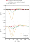 |
Fig. 2 Quadrupole moment of the real-space CCF for voids in the true cosmology (red) and a fiducial cosmology with ε = 1.053 and q = 1 (yellow and green). The yellow line is the assumed case where voids move under AP distortion in the same way as halos, while the green line is the more realistic case where voids are found in the distorted halo field. There is a clear additional effect that imprints a signal in ξrr when voids are found in a distorted field. For demonstration purposes, the data shown here were obtained using voxel voids described in Sect. 4.2, but similar results apply for all void finders and can be found in Appendix B. The lower panel shows the same test on simulation boxes with different densities, including Quijote halos subsampled to half the original density, and NSERIES4 galaxies with 1.2 times the density of Quijote. |
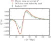 |
Fig. 3 Quadrupole moment of the redshift-space CCF for voids in a fiducial cosmology that differs from the truth (ε = 1.053 and q = 1). In red we plot the theoretical prediction calculated using an isotropic template ξrr. This fits the data in yellow, measured from a simulation in which both halos and voids have been moved by hand, while deviating significantly from the more realistic data in green, where voids are found in a distorted halo catalogue. As in Fig. 2, for simplicity only the case of voxel voids is shown here, though similar results apply to all void finders and can be found in Appendix B. |
3.3 Model inputs
A full evaluation of Eq. (12) requires the specification of the real-space CCF ξrr and the velocity distribution P(v‖, r). We now describe the details of how these are computed for the calculations performed in this paper.
3.3.1 Velocity distribution
We model the velocity distribution P(v‖, r) as an isotropic Gaussian distribution dependent on the distance from the void centre:
![Mathematical equation: $\[P\left(v_{\|}, r\right)=\frac{1}{\sqrt{2 ~\pi ~\sigma_{v_{\|}}^2(r)}} \exp \left\{-\frac{\left[v_{\|}-\mu_r v_{\mathrm{r}}(r)\right]^2}{2 \sigma_{v_{\|}}^2(r)}\right\}.\]$](/articles/aa/full_html/2024/11/aa51358-24/aa51358-24-eq20.png) (14)
(14)
This distribution depends on two functions to be specified: the coherent radial outflow velocity vr(r) and the velocity dispersion ![Mathematical equation: $\[\sigma_{v_{\|}}(r)\]$](/articles/aa/full_html/2024/11/aa51358-24/aa51358-24-eq21.png) .
.
The outflow velocity vr(r) is usually assumed to be related to the enclosed matter density profile Δ(r) for voids via a linearised form of the continuity equation, ![Mathematical equation: $\[v_{\mathrm{r}}(r)=-\frac{1}{3} f ~{ a ~H ~r } ~\Delta(r)\]$](/articles/aa/full_html/2024/11/aa51358-24/aa51358-24-eq22.png) , where f and a are the growth rate and scale factor, respectively. This approximation works reasonably well (e.g. Hamaus et al. 2014; Nadathur & Percival 2019), although Massara et al. (2022) highlighted shortcomings in some circumstances. The matter profile Δ(r) is in turn either determined from the monopole moment
, where f and a are the growth rate and scale factor, respectively. This approximation works reasonably well (e.g. Hamaus et al. 2014; Nadathur & Percival 2019), although Massara et al. (2022) highlighted shortcomings in some circumstances. The matter profile Δ(r) is in turn either determined from the monopole moment ![Mathematical equation: $\[\xi_0^{\mathrm{rr}}(r)\]$](/articles/aa/full_html/2024/11/aa51358-24/aa51358-24-eq23.png) of the real-space CCF via an assumed effective linear bias relationship (e.g. Pollina et al. 2017; Aubert et al. 2022; Hamaus et al. 2022; Schuster et al. 2023), or taken from a template function Δref calibrated from simulations (e.g. Nadathur et al. 2019b, 2020; Woodfinden et al. 2022). In the latter approach, as the template Δref(r) is empirically found to scale proportionally with the amplitude of matter density perturbations, such that
of the real-space CCF via an assumed effective linear bias relationship (e.g. Pollina et al. 2017; Aubert et al. 2022; Hamaus et al. 2022; Schuster et al. 2023), or taken from a template function Δref calibrated from simulations (e.g. Nadathur et al. 2019b, 2020; Woodfinden et al. 2022). In the latter approach, as the template Δref(r) is empirically found to scale proportionally with the amplitude of matter density perturbations, such that ![Mathematical equation: $\[\Delta^{\text {true }}(r)=\left(\sigma_8^{\mathrm{true}} / \sigma_8^{\mathrm{ref}}\right) \Delta^{\mathrm{ref}}\]$](/articles/aa/full_html/2024/11/aa51358-24/aa51358-24-eq24.png) (Nadathur et al. 2019b), where the superscripts true and ref refer to the true cosmological model and that of the simulation from which the template was calibrated. Together with the continuity equation, this empirical scaling results in the relationship
(Nadathur et al. 2019b), where the superscripts true and ref refer to the true cosmological model and that of the simulation from which the template was calibrated. Together with the continuity equation, this empirical scaling results in the relationship
![Mathematical equation: $\[\left(\frac{v_{\mathrm{r}}}{a H}\right)^{\mathrm{true}}=\frac{\left(f \sigma_8\right)^{\text {true }}}{\left(f \sigma_8\right)^{\mathrm{ref}}}\left(\frac{v_{\mathrm{r}}}{a H}\right)^{\mathrm{ref}},\]$](/articles/aa/full_html/2024/11/aa51358-24/aa51358-24-eq25.png) (15)
(15)
that is, the velocity profile inherits a dependence ∝ f σ8. We note that the aH factors on either side of the equation also allow for differences between the true effective redshift of the data and the simulation redshift used for template calibration to be included.
In this paper, we adopt a modification of the template calibration: instead of calibrating a template Δref(r) from simulations, we directly measure a velocity profile template ![Mathematical equation: $\[v_{\mathrm{r}}^{\mathrm{ref}}(r)\]$](/articles/aa/full_html/2024/11/aa51358-24/aa51358-24-eq26.png) . This means we can isolate imperfections in the CCF model that arise from the AP distortions of interest here from those that may be related to residual deviations from the assumption of purely linear dynamics relating vr and Δ. Nevertheless, we continue to assume that the scaling of vr with the growth factor f σ8 implied by Eq. (15) holds.
. This means we can isolate imperfections in the CCF model that arise from the AP distortions of interest here from those that may be related to residual deviations from the assumption of purely linear dynamics relating vr and Δ. Nevertheless, we continue to assume that the scaling of vr with the growth factor f σ8 implied by Eq. (15) holds.
In the same way, we also calibrate a template velocity dispersion function ![Mathematical equation: $\[\sigma_{v_{\|}}^{\mathrm{ref}}(r)\]$](/articles/aa/full_html/2024/11/aa51358-24/aa51358-24-eq27.png) , and take the true velocity dispersion to be proportional to this template, with a free amplitude that is treated as a nuisance parameter and marginalised over when reporting cosmological constraints (see Radinović et al. 2023, for details).
, and take the true velocity dispersion to be proportional to this template, with a free amplitude that is treated as a nuisance parameter and marginalised over when reporting cosmological constraints (see Radinović et al. 2023, for details).
In practice, the template functions are calibrated for voids with an average size defined by some chosen cuts on the void sample. The apparent size of voids in the real Universe, where q is unknown, may differ from the physical size of voids in the simulation, where q = 1, so the same apparent size cuts may result in a void sample of different average physical size in the two situations. To account for this, we allow the model functions in the true cosmology to differ from the reference templates through an isotropic rescaling of all distance scales, setting Xtrue(rtrue) = Xref(α* rtrue), where X represents the model function in question and α* is a free parameter.
If changes from the template occur purely due to the AP volume dilation, we should have ![Mathematical equation: $\[\alpha^*=q=q_{\perp}^{2 / 3} q_{\|}^{1 / 3}\]$](/articles/aa/full_html/2024/11/aa51358-24/aa51358-24-eq28.png) and the effect of such rescaling on the model in Eq. (12) is exactly cancelled by the opposite shift when the AP model is applied to the red-shift space CCF in the final step using Eq. (11). This ensures that the observed void size cannot be used as a standard ruler and no constraints on q are obtained. The same cancellation also automatically occurs in alternative approaches (e.g. Hamaus et al. 2022) in which distances from the void centre are always scaled in units of apparent void size. To allow for more general deviations in shape from the calibrated templates, we can also allow α* to differ from q, but in this case the two parameters remain very degenerate and so it is still not possible to constrain either of them.
and the effect of such rescaling on the model in Eq. (12) is exactly cancelled by the opposite shift when the AP model is applied to the red-shift space CCF in the final step using Eq. (11). This ensures that the observed void size cannot be used as a standard ruler and no constraints on q are obtained. The same cancellation also automatically occurs in alternative approaches (e.g. Hamaus et al. 2022) in which distances from the void centre are always scaled in units of apparent void size. To allow for more general deviations in shape from the calibrated templates, we can also allow α* to differ from q, but in this case the two parameters remain very degenerate and so it is still not possible to constrain either of them.
3.3.2 Real-space CCF
The predictions obtained from Eq. (12) and models related to it are most sensitive to the form of the real-space CCF ξrr(r), so this is the most important input to get right. Various approaches have been used to determine ξrr(r), including using an analytic formula (Hamaus et al. 2014), using a template calibrated from simulations (Nadathur et al. 2019b, 2020; Woodfinden et al. 2022), and determining it directly from data (Hamaus et al. 2022; Radinović et al. 2023). We will consider examples of the last two of these methods in the following.
The first, template-based, method involves using simulated mock data that is designed to approximately match the tracer number density and large-scale clustering amplitude of the real data. Through applying the void-finding and CCF measurement steps on such a mock, we can determine a reference template function ![Mathematical equation: $\[\xi_\mathrm{ref}^{\mathrm{rr}}\]$](/articles/aa/full_html/2024/11/aa51358-24/aa51358-24-eq29.png) . As the effects of RSD and AP distortions can be exactly removed in the mock where tracer velocities and the true cosmology are known, this template is usually perfectly isotropic to within measurement errors,
. As the effects of RSD and AP distortions can be exactly removed in the mock where tracer velocities and the true cosmology are known, this template is usually perfectly isotropic to within measurement errors, ![Mathematical equation: $\[\xi_{\mathrm{ref}}^{\mathrm{rr}}=\xi_{\mathrm{ref}}^{\mathrm{rr}}(r)\]$](/articles/aa/full_html/2024/11/aa51358-24/aa51358-24-eq30.png) . As for the velocity template functions above, we allow an arbitrary isotropic rescaling of distance scales,
. As for the velocity template functions above, we allow an arbitrary isotropic rescaling of distance scales, ![Mathematical equation: $\[\xi_{\text {true }}^{\mathrm{rr}}\left(r^{\mathrm{true}}\right)=\xi_{\mathrm{ref}}^{\mathrm{rr}}\left(\alpha^* r^{\mathrm{ref}}\right)\]$](/articles/aa/full_html/2024/11/aa51358-24/aa51358-24-eq31.png) , which ensures that the template function is not used as a cosmological standard ruler.
, which ensures that the template function is not used as a cosmological standard ruler.
As the reference template function is isotropic, the template-based model relies on the assumption that the AP effect on void-finding does not introduce anisotropies in the true real-space CCF. The model also implicitly assumes that AP distortions can be modelled as though void centres move as galaxy or halo tracers. We show above that these two assumptions do not hold: the performance of the template-based model then allows us to quantify the effect these assumptions have on the final model performance.
The second approach involves determining the real-space CCF ξrr(r) from the data. Hamaus et al. (2022) do this by using the redshift-space data to measure the projected CCF ξp(s⊥), which is independent of RSD effects, and using a deprojection technique (Pisani et al. 2014) to obtain the real-space CCF. The deprojection step assumes spherical symmetry of the realspace CCF, and therefore suffers from the same limitations with respect to the AP effect as the template method. Radinović et al. (2023) propose a different method, which is based upon a reconstruction technique to approximately remove RSD from the galaxy catalogue before void-finding; using this reconstructed catalogue we can measure ![Mathematical equation: $\[\xi_{\mathrm{fid}}^{\mathrm{rr}}(\mathbf{r})\]$](/articles/aa/full_html/2024/11/aa51358-24/aa51358-24-eq32.png) in the fiducial cosmology. Radinović et al. (2023) demonstrated that this method can remove the effects of RSD to recover the real-space CCF sufficiently well for modelling purposes. We will assume that this RSD removal can be performed perfectly, with no residuals. This is not a fully realistic assumption in practice, but it helps us to separate out the additional AP effect we wish to determine here from any possible confounding RSD residuals. We will therefore use the known tracer velocities in our simulations to exactly subtract RSD in determining
in the fiducial cosmology. Radinović et al. (2023) demonstrated that this method can remove the effects of RSD to recover the real-space CCF sufficiently well for modelling purposes. We will assume that this RSD removal can be performed perfectly, with no residuals. This is not a fully realistic assumption in practice, but it helps us to separate out the additional AP effect we wish to determine here from any possible confounding RSD residuals. We will therefore use the known tracer velocities in our simulations to exactly subtract RSD in determining ![Mathematical equation: $\[\xi_{\mathrm{fid}}^{\mathrm{rr}}(\mathbf{r})\]$](/articles/aa/full_html/2024/11/aa51358-24/aa51358-24-eq33.png) , rather than using approximate reconstruction methods.
, rather than using approximate reconstruction methods.
From the measured ![Mathematical equation: $\[\xi_{\mathrm{fid}}^{\mathrm{rr}}(\mathbf{r})\]$](/articles/aa/full_html/2024/11/aa51358-24/aa51358-24-eq34.png) and for given AP scaling parameters q⊥ and q‖, we infer the true real-space CCF using:
and for given AP scaling parameters q⊥ and q‖, we infer the true real-space CCF using:
![Mathematical equation: $\[\xi_{\text {true }}^{\mathrm{rr}}\left(r_{\|}^{\mathrm{true}}, r_{\perp}^{\mathrm{true}}\right)=\xi_{\mathrm{fid}}^{\mathrm{rr}}\left(\frac{r_{\|}^{\mathrm{true}}}{q_{\|}}, \frac{r_{\perp}^{\mathrm{true}}}{q_{\perp}}\right).\]$](/articles/aa/full_html/2024/11/aa51358-24/aa51358-24-eq35.png) (16)
(16)
Importantly, if void-finding in the AP-distorted galaxy or halo field introduces additional anisotropies beyond those included in the simple model where void positions transform in the same way as tracers, as indicated by Fig. 2, these are automatically included in the measured ![Mathematical equation: $\[\xi_{\mathrm{fid}}^{\mathrm{rr}}(\mathbf{r})\]$](/articles/aa/full_html/2024/11/aa51358-24/aa51358-24-eq36.png) via Eq. (16). That is, even when the correct q⊥ and q‖ parameters corresponding to the true cosmology are used in Eq. (16), the resulting
via Eq. (16). That is, even when the correct q⊥ and q‖ parameters corresponding to the true cosmology are used in Eq. (16), the resulting ![Mathematical equation: $\[\xi_{\text {true }}^{\mathrm{rr}}\]$](/articles/aa/full_html/2024/11/aa51358-24/aa51358-24-eq37.png) function that is obtained need not be spherically symmetric. Anisotropies due to void-finding are thus ‘carried through’ the model computation in Eq. (12).
function that is obtained need not be spherically symmetric. Anisotropies due to void-finding are thus ‘carried through’ the model computation in Eq. (12).
In Fig. 4, we compare the model predictions using the possibly anisotropic ξrr determined from data and those obtained when assuming an isotropic ξrr taken from a template in a fixed cosmology. The results show that assuming isotropy of ξrr predicts a much greater model sensitivity to the AP parameter ratio ε = q⊥/q‖, particularly in the quadrupole moment. This is because this approach neglects the anisotropic selection effect of void-finding performed in a distorted tracer field, which tends to partially cancel the anisotropy introduced in the CCF. We show below that accounting for the anisotropic effect in void-finding results in much more accurate model predictions when ε ≠ 1.
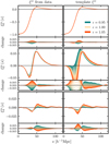 |
Fig. 4 Theoretical redshift-space CCF calculated for a range of fiducial cosmologies. The left-hand side shows how the theory responds to changes in the AP distortion parameter ε when the real-space CCF ξrr comes from the data, while the right-hand side shows the same for the case when ξrr is given as a template from simulations. From top to bottom, the three large panels show the monopole, quadrupole, and hexadecapole, while the residuals show the difference between the multipoles at a given ε and the multipoles when ε = 1. |
4 Methods
4.1 Simulations
For the analysis presented, we made use of 200 Quijote simulations6 (Villaescusa-Navarro et al. 2020) at redshift z = 0.5, with a box size of side L = 1000 h−1 Mpc. All of the boxes are at the fiducial Quijote cosmology, a flat ΛCDM cosmology with Ωm = 0.3175, Ωb = 0.049, h = 0.6711, ns = 0.9624, σ8 = 0.834. Despite our theory describing the void-galaxy CCF, we make use of the provided halo catalogues, with friends-of-friends (FoF) halos found with a halo finder implemented in Pylians37. This is equivalent to assuming every halo has one central galaxy, resembling a typical sample of luminous red galaxies (LRGs), which have a low fraction of satellite galaxies.
Each halo catalogue contains positions and velocities for about 3.09 · 105 halos in real space, corresponding to a number density of 3.09 · 10−4 h3Mpc−3. We used the provided halo velocities to construct corresponding redshift-space halo catalogues using Eq. (9) and assuming a line of sight along the direction of the z-axis of the box.
To avoid converting Cartesian positions of halos into angles and redshift, and reconverting them back into Cartesian coordinates while assuming a different cosmology, we instead stretched the simulation boxes directly. To do this, we applied the AP scaling factors q‖ and q⊥ to the halo positions in both real and redshift space, keeping the z-axis as the LoS direction and using Eqs. (5) and (6). In the case where the scaling factors are greater than one, we first duplicated the boxes along all the axes to make sure the entire box volume remained filled after compression. Finally, we cut the box down to its original size of 1000 h−1 Mpc.
This process results in cubic boxes which no longer satisfy periodic boundary conditions. While we can mostly ignore this for the purposes of void finding, we in general do not trust the results near the edges of the box. Therefore, for the purpose of measuring the CCF and velocity profiles, we conservatively cut 150 h−1 Mpc on all sides of the box, which is a scale greater than the largest void-galaxy pair separations considered. This leaves us with a volume that is about three times smaller than the original box volume.
We consider two groups of cases for the choice of q‖ and q⊥: flat ΛCDM cosmologies with different values of Ωm and cosmologies corresponding to isovolumetric distortion (q = 1 and ε ≠ 1). All combinations of q‖ and q⊥ (and ε and q) used in this paper are given in Table 1, along with the corresponding Ωm values for the FlatΛCDM cosmologies. In the case of isovolumetric distortions, we consider a more general case where a given combination of q‖ and q⊥ can arise from different combinations of parameters in different cosmologies. Therefore, we refrain from listing any cosmological parameters for those combinations in the table.
Combinations of Alcock–Paczyński scaling parameters used in the analysis.
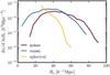 |
Fig. 5 Void size function for different void finders. We plot only one void size function for the two ZOBOV-based finders since the only difference between them is the void centre definition, and not the number of voids or their sizes. |
4.2 Void finding
The process of void finding can be conceptualised as a nonlinear transformation of the tracer field, leading to the identification of under-dense regions. While different void-finding algorithms all aim to recover these under-dense regions, they all employ different methodologies, resulting in vastly different voids, with different positions and statistical properties. In this paper, we focus on four void finders, which use three different algorithms, and explored how the AP effect influences the properties and characteristics of the voids identified by these algorithms.
The first two algorithms, ZOBOV (Neyrinck 2008) and voxel (Nadathur et al. 2019c), use a watershed-based technique, while the spherical void finder is based on the excursion set formalism (Banerjee & Dalal 2016). Here we will present a short overview of all of these algorithms as they are used on cubic simulation boxes.
4.2.1 ZOBOV
ZOBOV (Neyrinck 2008) is a watershed void-finder that uses a Voronoi tessellation approach to estimate the density field. In this approach the cosmological volume is divided such that each tracer particle is assigned a Voronoi cell, an area of space which is closer to that specific particle than it is to any other. These cells vary in size, with larger cells corresponding to regions where tracer particles are further away from each other, and smaller cells indicating areas of higher density (or closer tracer proximity).
The volume of the Voronoi cells helps us estimate the density field (ρ ∝ 1/V), as the largest cells pinpoint the locations of local minima, which serve as the starting points for the watershed algorithm. Additional neighbouring cells are progressively included in the void’s volume, with their densities increasing until a cell with lower density (a saddle point) is encountered. As this approach results in irregular void volumes, it is helpful to define an effective void radius Rv as the radius of a sphere with the same volume as the void:
![Mathematical equation: $\[R_{\mathrm{v}}=\left(\frac{3}{4 \pi} \sum_i V_i\right)^{\frac{1}{3}},\]$](/articles/aa/full_html/2024/11/aa51358-24/aa51358-24-eq38.png) (17)
(17)
where Vi is the volume of the i-th Voronoi cell, and the sum goes over all the cells belonging to the void. From here we can choose one of two different ways of estimating the void centre: circumcentre – used in the REVOLVER8 (Nadathur et al. 2019c) void-finding package – and barycentre – used in the VIDE9 (Sutter et al. 2015) void finder.
In the REVOLVER circumcentre definition, we find the four most under-dense mutually adjacent Voronoi cells belonging to the void. The tracer particles belonging to them form a tetrahedron, the circumcentre of which is defined as the centre of the void. Voids defined in this way naturally tend to be particularly under-dense in the centre, going down to δ = −1, and have a characteristic knee in the density profile, corresponding to the four tracer particles used to define the centre.
The Void IDentification and Examination toolkit (VIDE; Sutter et al. 2015) defines the location of the void centre as the volume-weighted barycentre of all the tracer particles belonging to the void. This gives us a nonlocal definition of the void centre and thus, while the voids identified by REVOLVER and VIDE are identical, the properties of the CCF measured using void centre positions differ significantly.
As void finding on a discrete tracer field can result in many small, spurious voids, we impose a selection criterion on our voids, removing all voids with a radius Rv smaller than 30 h−1 Mpc. This also removes true small voids which are mostly governed by nonlinear evolution and whose properties are not accurately described by the model given in Sect. 3.
4.2.2 voxel
Unlike ZOBOV, voxel is a void-finding algorithm that uses a particle-mesh interpolation technique to accurately estimate the density field. In this approach, tracers are placed on a three-dimensional grid of cells (voxels), with the grid size determined by the average number density of tracers ![Mathematical equation: $\[\bar{n}\]$](/articles/aa/full_html/2024/11/aa51358-24/aa51358-24-eq39.png) , such that the side-length of each voxel is
, such that the side-length of each voxel is ![Mathematical equation: $\[a_{\mathrm{vox}}=0.5~(4 \pi \bar{n} / 3)^{-1 / 3}\]$](/articles/aa/full_html/2024/11/aa51358-24/aa51358-24-eq40.png) , and the density is proportional to the number of tracers in the voxel. This interpolation scheme is easily parallelisable and faster than other density estimation methods, such as the one used in ZOBOV, scaling simply as the number of tracers, ∝ N.
, and the density is proportional to the number of tracers in the voxel. This interpolation scheme is easily parallelisable and faster than other density estimation methods, such as the one used in ZOBOV, scaling simply as the number of tracers, ∝ N.
Following the estimation of the density field, a Gaussian filter with a smoothing length ![Mathematical equation: $\[r_{\mathrm{s}}=\bar{n}^{-1 / 3}\]$](/articles/aa/full_html/2024/11/aa51358-24/aa51358-24-eq41.png) is applied and voids are identified as local minima within this smoothed density distribution. To determine the size and non-overlapping boundaries of each void, a watershed algorithm progressively includes neighbouring voxels until a critical point is reached where the density of the next cell is lower than that of the previous one. The centre of a voxel void is naturally defined as the position of the lowest density voxel belonging to it. As this is a locally defined centre, it is very sensitive to small-scale fluctuations of the density field; however, this does not seem to significantly affect the statistical properties of voxel voids.
is applied and voids are identified as local minima within this smoothed density distribution. To determine the size and non-overlapping boundaries of each void, a watershed algorithm progressively includes neighbouring voxels until a critical point is reached where the density of the next cell is lower than that of the previous one. The centre of a voxel void is naturally defined as the position of the lowest density voxel belonging to it. As this is a locally defined centre, it is very sensitive to small-scale fluctuations of the density field; however, this does not seem to significantly affect the statistical properties of voxel voids.
We once again find irregularly shaped voids and assign each an effective radius
![Mathematical equation: $\[R_{\mathrm{v}}=\left(\frac{3}{4 ~\pi} N_{\mathrm{vox}} V_{\mathrm{vox}}\right)^{\frac{1}{3}} \text {, }\]$](/articles/aa/full_html/2024/11/aa51358-24/aa51358-24-eq42.png) (18)
(18)
where Nvox is the number of voxels belonging to the void, and Vvox is the voxel volume. Just like for ZOBOV, we impose a radius cut on the voxel void catalogue. To keep the comparison easier, we use the same criterion of 30 h−1 Mpc and remove any voids with a radius smaller than that.
Though in this work we were limited to cubic boxes, in Fraser et al. (2024) the voxel algorithm was updated to handle non-cubic periodic boundary conditions. This facilitates the identification of voids in the distorted boxes without the need for the trimming procedure described in Sect. 4.1.
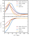 |
Fig. 6 Radial velocity and normalised line-of-sight velocity dispersion templates for different void finders. The templates are taken at a reference cosmology that matches the truth, presenting an idealised scenario. |
4.2.3 Spherical void finder
The spherical void finder used in this paper is implemented in the Pylians3 library10, and identifies non-overlapping spherical underdensities. As input, it requires a list of radii and an enclosed-overdensity threshold Δv which will be used to define a void. For the analysis presented here, we used a threshold of Δv = −0.7.
The void finder starts by placing tracer particles on a grid, and then smoothing the field with a top-hat filter of radius Rv, where Rv is the largest void radius in the input list. It then identifies all regions where the smoothed enclosed overdensity is below the threshold. Going from the most under-dense of these regions, we define a region as a void if it does not overlap with an already defined void. Though these voids can in principle have radii larger than the top-hat smoothing scale, they are all assigned the same radius Rv. The smoothing and identification process is then repeated for all the given void radii, from largest to the smallest, until we have a list of non-overlapping voids which fill the entire cosmological volume.
The voids we obtain in this way are effectively binned in radius, with the bins defined by the input list. For the analysis presented here, we used only the radius bin 27 ≤ Rv < 30 h−1 Mpc to calculate the CCF and the velocity template functions. It is useful to note that, while void radii of the various watershed algorithms can be roughly compared, radii of spherical voids have a different definition and therefore cannot be trivially compared to the watershed ones.
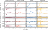 |
Fig. 7 Data and the model for all void finders considered in the paper, calculated in the true cosmology. We see the differences in shapes of various voids, such as the characteristic knee in the monopole of ZOBOV voids from REVOLVER, and the sharp features of spherical voids. |
4.3 Measuring velocity templates
Using the real-space positions of voids and halos in the true cosmology, and with the available halo peculiar velocities, we measured the radial outflow velocity and the LoS velocity dispersion. In practice, these templates would be measured from a simulation that is at some reference cosmology and does not contain AP distortion. However, since we instead measure them at the true cosmology, we construct an idealised scenario where the reference cosmology happens to be matching the true one (meaning that the simulation perfectly describes the Universe). We do this to demonstrate that the effect of AP distortions on void finding is there even in an ideal scenario, where we have perfect templates that match the truth.
To measure radial velocities around voids, the voids are stacked and the radial component of the halo velocities around them are binned in spherical shells, while averaging over all the void-halo pairs in the bin regardless of angle μ. This gives slightly different velocity profiles ![Mathematical equation: $\[v_{\mathrm{r}}^{\mathrm{ref}}(r)\]$](/articles/aa/full_html/2024/11/aa51358-24/aa51358-24-eq43.png) for each void finder, as seen in the top panel of Fig. 6. Regardless of their differences, the main feature is present in all: a peak around the steep edge of the void, which indicates a coherent radial outflow form the centre of the void. The reference velocity templates for each void type are rescaled according to Eq. (15) to obtain the model vr(r) used in Eq. (14) for the velocity probability distribution function (PDF).
for each void finder, as seen in the top panel of Fig. 6. Regardless of their differences, the main feature is present in all: a peak around the steep edge of the void, which indicates a coherent radial outflow form the centre of the void. The reference velocity templates for each void type are rescaled according to Eq. (15) to obtain the model vr(r) used in Eq. (14) for the velocity probability distribution function (PDF).
To obtain the dispersion profile, we compute the modulus of the halo velocity in each of the bins, ⟨|v|2⟩, and thus measure (see Fiorini et al. 2022)
![Mathematical equation: $\[\sigma_{v_{\|}}(r)=\sqrt{\frac{\left.\left.\langle | \mathbf{v}\right|^2\right\rangle-v_{\mathrm{r}}^2}{3}},\]$](/articles/aa/full_html/2024/11/aa51358-24/aa51358-24-eq44.png) (19)
(19)
for each void sample, which are shown in the bottom panel of Fig. 6 (normalised by the dispersion ![Mathematical equation: $\[\sigma_v \equiv \sigma_{v_{\|}}(r \rightarrow \infty)\]$](/articles/aa/full_html/2024/11/aa51358-24/aa51358-24-eq45.png) at large scales). We define the reference templates
at large scales). We define the reference templates ![Mathematical equation: $\[\sigma_{v_{\|}}^{\mathrm{ref}}(r)\]$](/articles/aa/full_html/2024/11/aa51358-24/aa51358-24-eq46.png) from these measured functions, leaving the amplitude σv as a free parameter.
from these measured functions, leaving the amplitude σv as a free parameter.
4.4 Measuring the void-halo CCF
After again stacking all voids that survived the radius cuts, as well as removing any voids near the edges of the simulation box (see Sect. 4.1), we used a modified and Python-wrapped version of CUTE11 (Correlation Utilities and Two point Estimation; Alonso 2012) to count void-halo pairs DvDg. It estimates the CCF via:
![Mathematical equation: $\[\xi(r, \mu)=\frac{V}{N_{\mathrm{v}} N_{\mathrm{g}}} \frac{D_{\mathrm{v}} D_{\mathrm{g}}(r, \mu)}{v(r, \mu)},\]$](/articles/aa/full_html/2024/11/aa51358-24/aa51358-24-eq47.png) (20)
(20)
where V is the box volume, Nv and Ng are the numbers of voids and galaxies, respectively, and v = 4πr2 ΔrΔμ is the volume of the ΔrΔμ bin. We used 100 angular bins in range μ ∈ (0, 1), and 30 radial bins up to r = 120h−1Mpc. Correlating the voids with real-space halos gives us ξrr, while correlating the same voids with redshift-space halos gives us ξrs. This process is applied to all 200 Quijote mocks, and the resulting CCFs are averaged over these 200 mock realisations.
The CCF measurement for both real and redshift space is done for all of the fiducial cosmologies listed in Table 1, with the one done at the true cosmology (no AP effect) serving also as a template ![Mathematical equation: $\[\xi_{\mathrm{rr}}^{\mathrm{ref}}\]$](/articles/aa/full_html/2024/11/aa51358-24/aa51358-24-eq48.png) . As with the velocity, these templates are then at the true cosmology and present an idealised scenario.
. As with the velocity, these templates are then at the true cosmology and present an idealised scenario.
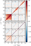 |
Fig. 8 Normalised data-only (top) and full (bottom) covariance matrix. We see that the off-diagonal correlation structure is much less pronounced in the full covariance than in the data-only one. |
4.5 Covariance matrix
As we consider two distinct cases, ξrr from data or as a template, we construct two covariance matrices. When ξrr is supplied as a template, the covariance matrix is the standard, data-only covariance. It is constructed from Nm = 200 mocks, using the equation
![Mathematical equation: $\[\mathrm{C}_{i j}^{\mathrm{data}}=\frac{1}{N_{\mathrm{m}}-1} \sum_{k=1}^{N_{\mathrm{m}}}\left(\xi_i^{\mathrm{rs}(k)}-\left\langle\xi^{\mathrm{rs}}{ }_i\right\rangle\right)\left(\xi_j^{\mathrm{rs}(k)}-\left\langle\xi^{\mathrm{rs}}{}_j\right\rangle\right),\]$](/articles/aa/full_html/2024/11/aa51358-24/aa51358-24-eq49.png) (21)
(21)
where ![Mathematical equation: $\[\xi_i^{(k)}\]$](/articles/aa/full_html/2024/11/aa51358-24/aa51358-24-eq50.png) is the ith bin of the redshift-space CCF for the kth mock, while ⟨ξrs⟩ is the mean over all Nm mocks. A covariance matrix constructed like this represents the error budget for a volume of (700h−1 Mpc)3, which is the volume of one mock after we cut out the edges (see Sect. 4.1). For an easier demonstration of the issues we present in this paper, we have chosen to rescale the covariance to a more realistic survey volume. We chose a DESI-like survey (Aghamousa et al. 2016), with a volume about 25 times that of our cut simulation box12, which means we divide the covariance in Eq. (21) by 25, assuming a linear scaling with volume.
is the ith bin of the redshift-space CCF for the kth mock, while ⟨ξrs⟩ is the mean over all Nm mocks. A covariance matrix constructed like this represents the error budget for a volume of (700h−1 Mpc)3, which is the volume of one mock after we cut out the edges (see Sect. 4.1). For an easier demonstration of the issues we present in this paper, we have chosen to rescale the covariance to a more realistic survey volume. We chose a DESI-like survey (Aghamousa et al. 2016), with a volume about 25 times that of our cut simulation box12, which means we divide the covariance in Eq. (21) by 25, assuming a linear scaling with volume.
When the real-space CCF ξrr is taken from the data itself, the theory calculated this way is naturally correlated with the data. This correlation needs to be accounted for and added into the covariance. We can write (Radinović et al. 2023):
![Mathematical equation: $\[\begin{aligned}\mathrm{C}(\text {data}- \text {theory})=~ & \mathrm{C}(\text {data})+\mathrm{C}(\text {theory}) \\& -2 \mathrm{C}(\text {data, theory}),\end{aligned}\]$](/articles/aa/full_html/2024/11/aa51358-24/aa51358-24-eq51.png) (22)
(22)
where the first term is the one given by Eq. (21), the second is calculated in a similar way but with the theoretical ξrs instead of the measured one, while the last term captures the cross-covariance between the two. This cross-covariance term brings down the total variance and therefore results in tighter error bars.
It would be logical to conclude that using the full covariance Ctot would then result in tighter constraints on ε, but one look at Fig. 4 shows why such a conclusion might be wrong. Namely, our model responds more strongly to changes in ε when we supply a template real-space CCF, resulting in tighter constraints (see Sect. 5).
Covariances estimated like this, using a finite number of mocks, are inherently uncertain. Therefore, we have to propagate this uncertainty to the likelihood, which we do using the prescription described in Percival et al. (2022). We write the likelihood as
![Mathematical equation: $\[\log ~\mathcal{L}=-\frac{m}{2} ~\log~ \left(1+\frac{\chi^2}{N_{\mathrm{m}}-1}\right),\]$](/articles/aa/full_html/2024/11/aa51358-24/aa51358-24-eq52.png) (23)
(23)
with χ2 given by
![Mathematical equation: $\[\chi^2=\left(\xi_{\text {theory }}^{\mathrm{rs}}-\xi_{\text {data }}^{\mathrm{rs}}\right) \mathrm{C}^{-1}\left(\xi_{\text {theory }}^{\mathrm{rs}}-\xi_{\mathrm{data}}^{\mathrm{rs}}\right)^{\mathrm{T}}.\]$](/articles/aa/full_html/2024/11/aa51358-24/aa51358-24-eq53.png) (24)
(24)
The power-law index m is defined as:
![Mathematical equation: $\[m=n_\theta+2+\frac{N_{\mathrm{m}}-1+B\left(n_{\mathrm{d}}-n_\theta\right)}{1+B\left(n_{\mathrm{d}}-n_\theta\right)},\]$](/articles/aa/full_html/2024/11/aa51358-24/aa51358-24-eq54.png) (25)
(25)
![Mathematical equation: $\[B=\frac{N_{\mathrm{m}}-n_{\mathrm{d}}-2}{\left(N_{\mathrm{m}}-n_{\mathrm{d}}-1\right)\left(N_{\mathrm{m}}-n_{\mathrm{d}}-4\right)},\]$](/articles/aa/full_html/2024/11/aa51358-24/aa51358-24-eq55.png) (26)
(26)
where the Nm = 200 is, as before, the number of mocks used, and nd = 90 is the number of data points (30 radial bins for three multipoles). Finally, nθ is the number of independent parameters. Though our parameter space is given by five parameters, {f σ8, σv, ε, q, α*}, q and α* are completely degenerate, which leaves us with nθ = 4.
To maximize the likelihood given in Eq. (23), we sample the parameter space using the Monte Carlo Markov Chain (MCMC) sampler in Cobaya13 (Torrado & Lewis 2021), with the model and likelihood implemented in victor14. Convergence of the chains was ensured using the Gelman-Rubin R − 1 statistic, using the convergence criterion R − 1 < 0.01, and 20% of the initial steps were discarded as burn-in.
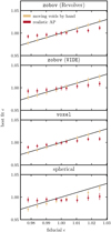 |
Fig. 9 Constraints on ε when assuming different fiducial flat ΛCDM cosmologies (top part of Table 1). Yellow points are for the test case where both halos and voids were moved by hand, while the red points are for a more realistic case, where voids were found in the distorted halo field. The x-axis shows the ε corresponding to the fiducial cosmology, while the y-axis is the best fit. The diagonal black line represents the point where the best-fit ε matches the fiducial one. |
5 Response of void finders to AP distortions
In Sect. 3 we demonstrated qualitatively that disregarding the effect of AP distortions on void finding will likely lead to a biased result. Now we will quantify those biases using a template approach, as well as propose a couple of methods to mitigate the issue.
5.1 Isotropic real-space CCF (template)
We first constructed a scenario in which the assumption of void movement under AP is true by applying an AP shift to both halos and voids for nine fiducial flat ΛCDM cosmologies (top part of Table 1). Using an isotropic template ξrr to calculate the theory, we obtained constraints on ε that are given in yellow in Fig. 9, where we see that ε is successfully recovered for all of the fiducial cosmologies and across almost all void finders15. This is show by the yellow points, which all following the black line for which the best-fit ε is equal to the fiducial one, meaning that the true cosmology is successfully recovered. This means that the model indeed works well if the assumption on void movement under AP is true.
Next we took a more realistic approach, allowing AP shifts in halo positions and performing void finding on this AP distorted halo catalogue, which is equivalent to the application of the analysis to real data. We again used a template ξrr to calculate the theory, like in the previous case, so the results are expected to match the previous ones if the assumption that voids move like tracers under AP is true. However, in Fig. 9 (in red) we explicitly see that the results differ significantly and that this approach leaves us with a strong bias when the fiducial cosmology is different than the truth. While these results are unsurprising given Figs. 2 and 3, here we see that not only are the results biased for all void finders, but this approach also strongly favours values of ε closer to one, regardless of the fiducial cosmology.
This appears to be a direct result of the additional signal in the CCF seen in Sect. 3, which is induced by the void finder response to the AP distortion in tracer positions. As the effect is most prominent in the quadrupole, we expect that any method of obtaining the real-space CCF which excludes this quadrupole will return a biased result. In this paper we present two ways that attempt to mitigate this issue without resorting to analytic modelling of the effect.
5.2 Approach 1: Anisotropic real-space CCF
Since the effect of AP distortions on void finding leaves an imprint in the real-space CCF that is not accounted for with an isotropic template CCF (Fig. 2), we can circumvent the issue by taking the anisotropic real-space CCF ξrr directly from the data. For simplicity, in the current work, we measure the real-space CCF in the simulations, but note that this procedure is also generalisable to real data applications, where approximation to the real-space CCF can be obtained from the data using reconstruction, as demonstrated in Radinović et al. (2023). Whatever the case, this ensures that the additional effect will be included and can be propagated directly to the redshift-space CCF via the RSD mapping. Additionally, as both the model input ξrr and the data vector ξrs come from the same set of voids and halos, the model prediction and data will themselves be correlated and, to account for this, we use the full covariance matrix Ctot as defined in Eq. (22).
Because the real-space CCF is measured in the fiducial cosmology, we do not perform any AP rescaling on it. Instead, the only part of Eq. (12) that needs to be rescaled is the velocity PDF, which is in the reference cosmology. This means that the constraining power on ε is greatly reduced, since the AP distortion on ξrr is not being modelled, and we are only getting constraints from the effect of AP distortion to the velocity PDF. The result of applying this approach to all the fiducial cosmologies given in Table 1 is shown in green, in Fig. 10, alongside the results from the previous section (red). Though the constraint on ε is weaker, we are closer to recovering the fiducial values, in some cases even for cosmologies very far from the true one (extreme points in the right panel of Fig. 10). The REVOLVER implementation of ZOBOV in particular responds well to this method, recovering the correct value of ε to within 1σ in all cases. In general, all of the void finders seem to handle isovolumetric distortion well, perhaps due to the velocity templates being better suited for those cases. This is particularly obvious for the spherical void finder, which does better only for isovolumetric distortions, while the flat ΛCDM cosmologies remain seemingly insensitive to ε. voxel and VIDE show mixed results, performing poorly for fiducial ε values much greater than one, but well otherwise, with voxel performing a little better than VIDE. This indicates that higher values of ![Mathematical equation: $\[\Omega_{\mathrm{m}}^{\mathrm{fid}}\]$](/articles/aa/full_html/2024/11/aa51358-24/aa51358-24-eq56.png) are a safer assumption for these void finders.
are a safer assumption for these void finders.
We can think of AP distortions to the CCF depending on shifts in both void and tracer positions, which are described in Sect. 2.1, and a more complicated effect, which is a function of the specific void-finding algorithm used, and results in the differences we see in Figs. 2 and 3. The success of the approach presented here suggests that these effects are at least somewhat separable; rescaling the CCF using AP scaling parameters accounts for the AP shifts, while the effect on void finding is left to propagate through the RSD mapping, and is correctly included in the calculated redshift-space CCF.
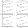 |
Fig. 10 Constraints on ε when assuming different cosmologies: a flat ΛCDM on the left and fixed q = 1 on the right. Red points are obtained when using a template ξrr (and match the red points in Fig. 9), while the green ones are obtained when ξrr is taken from data. The x-axis shows the ε corresponding to the fiducial cosmology, while the y-axis is the best fit. The diagonal black line represents the point where the best-fit ε matches the fiducial one. |
5.3 Approach 2: Iterative template-based modelling
While the first approach seems to work well, it does result in weaker constraints, and depends strongly on our ability to accurately obtain the real-space CCF using, for example, reconstruction. An alternative presents itself in Fig. 9, where we see that, although the red points are biased, the bias itself depends on ε. Iterating using the template approach, we can try to recover the true cosmology step by step, similarly to what was done in Beyond-2pt Collaboration (2024).
We start with a flat ΛCDM fiducial cosmology with ![Mathematical equation: $\[\Omega_{\mathrm{m}}^{\mathrm{fid}}\]$](/articles/aa/full_html/2024/11/aa51358-24/aa51358-24-eq57.png) = 0.2, which corresponds to q‖ = 0.9170 and q⊥ = 0.9583. We stretch the halo positions according to those values, and run all of our void-finding algorithms to obtain the void catalogues and, finally, data vectors. The real-space CCF and velocity profiles are supplied as templates, like in Sect. 5.1. This gives us a constraint on ε that can be translated into Ωm, which will be our new fiducial cosmology. From our new fiducial
= 0.2, which corresponds to q‖ = 0.9170 and q⊥ = 0.9583. We stretch the halo positions according to those values, and run all of our void-finding algorithms to obtain the void catalogues and, finally, data vectors. The real-space CCF and velocity profiles are supplied as templates, like in Sect. 5.1. This gives us a constraint on ε that can be translated into Ωm, which will be our new fiducial cosmology. From our new fiducial ![Mathematical equation: $\[\Omega_{\mathrm{m}}^{\mathrm{fid}}\]$](/articles/aa/full_html/2024/11/aa51358-24/aa51358-24-eq58.png) , we can in turn get new rescaling parameters using Eqs. (3) and (4), and the true value
, we can in turn get new rescaling parameters using Eqs. (3) and (4), and the true value ![Mathematical equation: $\[\Omega_{\mathrm{m}}^{\mathrm{true}}\]$](/articles/aa/full_html/2024/11/aa51358-24/aa51358-24-eq59.png) from the simulation. Because of the bias we find in Sect. 5.1, it is not enough to recover a value of ε that is consistent with one to within 1–2σ, we have to make sure we are actually close to the truth. Therefore, this process is repeated until the best-fit value of ε crosses the point of ε = 1.
from the simulation. Because of the bias we find in Sect. 5.1, it is not enough to recover a value of ε that is consistent with one to within 1–2σ, we have to make sure we are actually close to the truth. Therefore, this process is repeated until the best-fit value of ε crosses the point of ε = 1.
The results at each step are given in Fig. 11, with constraints on ε in the four left-most panels and constraints on Ωm in the right column. For ε we aim to recover back the fiducial value of ε that we put in by assuming a cosmology and stretching the simulation boxes accordingly. In essence, the x-axis represents our fiducial cosmology, and the y-axis tells us if that guess is correct. The spherical void finder, for example, very quickly returns ε = 1 even when our fiducial cosmology is very far from the truth. This would, in turn, result in a wrong estimate of Ωm, as we see in Fig. 11 (right panel). While choices like radius binning might affect the result to some degree, the spherical void finder seems inadequate for this specific approach, possibly due to the sharp features which are sensitive to noise.
The REVOLVER implementation of ZOBOV, on the other hand, gives an unbiased result but takes a lot of steps to reach it, while VIDE takes slightly fewer steps but results in more bias. Moreover, the biggest issue for both is that void finding itself is very time-consuming for tessellation based methods. A good compromise between speed and accuracy for this approach is the voxel void finder, which manages to quickly recover the correct value of Ωm to within 1σ, while running about ten times faster than ZOBOV. However, the difference in accuracy between the two ZOBOV void finders might provide an interesting insight into the issue, since the void-finding step is the same, with the only difference being in the centre definition: REVOLVER defines the centre using only four particles, while VIDE employs a more complicated approach, considering all of the particles belonging to the void. The point-based centre of REVOLVER voids might be better equipped to follow the AP shifts of galaxies, unlike voids with nonlocal centre definitions. Furthermore, it is likely that it is the density estimation step (which all of the void finders here employ) that ‘smears out’ the galaxy, and thus void, positions and affects the expected AP shifts. A topological void-finding algorithm, which works directly with galaxy positions without estimating the density field, could be an interesting avenue to follow in this case.
In general, the success of each void finder in this approach can be deduced already from the red points in Fig. 10, since they trace the possible path that the iterative approach can take. Thus, testing the suitability of new, different void finders to this approach can be done by repeating the analysis in Sect. 5.1.
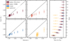 |
Fig. 11 Constraints on ε and Ωm obtained using iterative template-based modelling. The four panels on the left show best-fit ε values obtained at each step, while the right panel shows the resulting Ωm constraints, assuming a flat ΛCDM universe. The black vertical line is the true Ωm of the Quijote simulations, while the four diagonal black lines represent the points where best-fit ε matches the fiducial one. |
6 Conclusions
In this study, we investigated the effect of AP distortions on the void-galaxy cross-correlation function. Previous studies relied on an implicit assumption that the process of void finding is unaffected by AP distortions, with void positions in a given fiducial cosmology simply related by an AP shift to void positions in the true cosmology, similarly to galaxies. We show that this assumption is generally incorrect, especially when the fiducial cosmology differs significantly from the true one. This effect was also observed by Mao et al. (2017), who attributed it to a sparsity of tracers, though in our analysis we do not see any dependence on the number density of tracers (Fig. 2). This finding has important implications for the modelling of the void-galaxy CCF and the results of previous studies of the AP effect in voids that have recovered constraints on the AP distortion parameter ε. Although we mainly focused on template approaches to the CCF modelling in this study, we stress that this effect impacts all theoretical models of the void-galaxy CCF, and is present regardless of whether voids are located in real or redshift space. Despite this, the constraining power of voids, that is, the error on ε, is not likely to be affected if the iterative approach is used. Depending on the void finder used, previous constraints that recover ε = 1, which is where the chosen fiducial cosmology is very close to the true one, will be less affected; however, as seen in Fig. 10, this is not a guarantee that biases are not present. In particular, some previous studies (Hamaus et al. 2016; Nadathur et al. 2020; Aubert et al. 2022; Hamaus et al. 2020; Woodfinden et al. 2022) investigated the systematic error related to the choice of fiducial cosmology, and correctly accounted for this bias by including it in the total error budget.
A more appropriate treatment of this effect would require the development of a host of models for all of the different void finders, as the effect itself depends on the specific algorithm used. Alternatively, one could adopt a machine learning approach, in which a neural network could be trained to recognise the finder response to AP (Fraser et al. 2024). Though this approach has proven to work well, it is also finder specific, and is computationally intensive in its initial stages. In this paper, we instead proposed two methods that enable us to mitigate the effect of void-finder response to AP, while avoiding complicated modelling.
As the effect of AP distortions on void finding leaves an imprint in the real-space CCF, which is not accounted for with an isotropic CCF, we can circumvent the issue by estimating the real-space CCF directly from the data. This real-space CCF contains the anisotropies induced by the fiducial cosmology, helping us propagate the unknown contribution from the void finder response and recover unbiased cosmological parameters. This way we can recover the true ε values even when the fiducial cosmologies are very far from the true one. The disadvantages to this approach, however, are that it results in weaker constraints, and depends heavily on our ability to accurately obtain the real-space CCF (e.g. using reconstruction).
The second method we investigated is an iterative approach. We performed a full analysis using a fixed fiducial cosmology and, using the recovered value of ε, we redefined the fiducial cosmology (i.e. Ωm) iteratively until the new best-fit value crossed the point of ε = 1 (meaning an ε > 1 becomes ε < 1, or vice versa). We find that this approach works well in most cases, but depends to a large extent on the void finder in question. The spherical void finder converges quickly, but gives a very biased result; ZOBOV gives an unbiased result, but is very slow to converge; while the voxel void-finder is both fast to converge and gives unbiased results. A particular benefit of the iterative approach is that it can be easily applied to previous studies to ensure that the recovered parameters are unbiased, without sacrificing the constraining power.
Acknowledgements
SR acknowledges support from the Research Council of Norway through project 325113. SN acknowledges support from an STFC Ernest Rutherford Fellowship, grant reference ST/T005009/2. Research at Perimeter Institute is supported in part by the Government of Canada through the Department of Innovation, Science and Economic Development Canada and by the Province of Ontario through the Ministry of Colleges and Universities.
Appendix A Data vectors
For completeness, we show here all of the data vectors measured for the analysis presented in this paper. They cover all of the fiducial cosmologies listed in Table 1: the nine flat ΛCDM cosmologies are shown in Fig. A.1 and the 12 cosmologies with isovolumetric AP distortion are shown in Fig. A.2. The data vectors for all of the four void finders are comprised of a monopole, quadrupole, and hexadecapole moment, with the hexadecapole being largely dominated by noise. An exception to this is the voxel void finder, which seems to show a clear signal in the hexadecapole, even though it does not vary with ε.
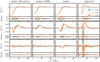 |
Fig. A.1 Data vectors for all of the void finders for different flat ΛCDM fiducial cosmologies (top part of Table 1). We see that the hexadecapole is almost completely noise dominated, while the monopole and quadrupole show a clear response to the change in ε and q. |
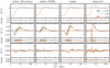 |
Fig. A.2 Data vectors for all of the void finders for different fiducial cosmologies with isovolumetric distortions (q = 1, lower part of Table 1). While the quadrupole shows a strong response to the change in ε, the monopole does not change significantly since the void size stays constant in the different cosmologies. |
Figure A.2 shows that when q is kept fixed, there is no significant change in the monopole, while the quadrupole contains the bulk of the information on the changing distortion parameter ε. This is expected as the monopole is mostly sensitive to the change in the overall volume of the void, while a changing ε only distorts the shape, which is described by the quadrupole. Indeed, in Fig. A.1, where ε and q both change, we see that the change in the overall void volume (or size) is evident in both the monopole and multipole.
Appendix B Voids in redshift space
In this appendix we show some additional results for the idealised test performed in Sect. 3.1. While in Sect. 3.1 we demonstrate the effect only for one of the void finders, here we show that it is an effect that persists in all of the algorithms that we investigate, excluding the possibility of a finder-specific error. In Fig. B.1 we show the quadrupoles of the real-space CCF we get when we assume voids move under AP distortion in the same way as halos compared to the case where voids are found in the distorted halo field, corresponding to the realistic scenario. The results given in Figs. 2 and 3 are in the third panel (voxel), but we see that the other void finders show the same trend, namely that AP distortions have smaller amplitude in reality (green) than expected (yellow).
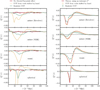 |
Fig. B.1 Quadrupole moments of the real and redshift-space CCFs for all void finders, with voids found in real space. Left: Quadrupoles of the real-space CCF in the true cosmology (red) and a fiducial cosmology with ε = 1.053 and q = 1 (yellow and green). The yellow line is the assumed case where voids move under AP distortion in the same way as halos, while the green line is the more realistic case where voids are found in the distorted halo field. Right: Quadrupoles of the redshift-space CCF in a fiducial cosmology which differs from the truth (ε = 1.053 and q = 1). In red we plot the theory prediction, calculated using a template ξrr. |
The results in Sect. 3.1 all have voids identified in real space, but void-finding can be run on the redshift-space catalogue as well. In this case the tracer positions contain RSD as well, introducing another source of anisotropy into the void shapes. This is evident in the left panel of Fig. B.2, where the quadrupole of the real-space CCF (now ξsr instead of ξrr) in the true cosmology is no longer zero and instead shows that voids are stretched along the line of sight. Despite these differences, we still see a large difference between the expected quadrupole in the fiducial cosmology (yellow, assuming voids move under AP in the same way as tracers) and the realistic one (green), showing that the effect also persists regardless of what space the voids are located in. In the right panel we again plot the measured redshift-space CCFs, as well as the model calculations. It is worth noting that, even in the idealised case, the model does not describe the data well, because there is a selection effect due to the voids having a preferred orientation, similarly to the voids in a fiducial cosmology with AP distortions. Unlike the AP, however, this selection effect cannot be attenuated or circumvented by the methods described in this paper.
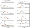 |
Fig. B.2 Quadrupole moments of the real and redshift-space CCFs for all void finders, with voids found in redshift space. Left: Quadrupoles of the real-space CCF in the true cosmology (red) and a fiducial cosmology with ε = 1.053 and q = 1 (yellow and green). The yellow line is the assumed case where voids move under AP distortion in the same way as halos, while the green line is the more realistic case where voids are found in the distorted halo field. Right: Quadrupoles of the redshift-space CCF in a fiducial cosmology which differs from the truth (ε = 1.053 and q = 1). In red we plot the theory prediction, calculated using a template ξrr. |
References
- Achitouv, I. 2019, Phys. Rev. D, 100, 123513 [NASA ADS] [CrossRef] [Google Scholar]
- Aghamousa, A., et al. 2016 [arXiv:1611.00036] [Google Scholar]
- Alam, S., Albareti, F. D., Allende Prieto, C., et al. 2015, ApJS, 219, 12 [Google Scholar]
- Alam, S., Aubert, M., Avila, S., et al. 2021, Phys. Rev. D, 103, 083533 [NASA ADS] [CrossRef] [Google Scholar]
- Alcock, C., & Paczynski, B. 1979, Nature, 281, 358 [NASA ADS] [CrossRef] [Google Scholar]
- Alonso, D. 2012, arXiv e-prints [arXiv:1210.1833] [Google Scholar]
- Alonso, D., Hill, J. C., Hložek, R., & Spergel, D. N. 2018, Phys. Rev. D, 97, 063514 [NASA ADS] [CrossRef] [Google Scholar]
- Aubert, M., Cousinou, M.-C., Escoffier, S., et al. 2022, MNRAS, 513, 186 [NASA ADS] [CrossRef] [Google Scholar]
- Banerjee, A., & Dalal, N. 2016, J. Cosmology Astropart. Phys., 2016, 015 [CrossRef] [Google Scholar]
- Beyond-2pt Collaboration, (Krause, E., et al.) 2024, arXiv e-prints [arXiv:2405.02252] [Google Scholar]
- Blanton, M. R., Bershady, M. A., Abolfathi, B., et al. 2017, AJ, 154, 28 [Google Scholar]
- Bonici, M., Carbone, C., Vielzeuf, P., et al. 2023, A&A, 670, A47 [NASA ADS] [CrossRef] [EDP Sciences] [Google Scholar]
- Cai, Y.-C., Taylor, A., Peacock, J. A., & Padilla, N. 2016, MNRAS, 462, 2465 [NASA ADS] [CrossRef] [Google Scholar]
- Chan, K. C., Hamaus, N., & Desjacques, V. 2014, Phys. Rev. D, 90, 103521 [NASA ADS] [CrossRef] [Google Scholar]
- Chuang, C.-H., Kitaura, F.-S., Liang, Y., et al. 2017, Phys. Rev. D, 95, 063528 [NASA ADS] [CrossRef] [Google Scholar]
- Colberg, J. M., et al. 2008, MNRAS, 387, 933 [NASA ADS] [CrossRef] [Google Scholar]
- Contarini, S., Verza, G., Pisani, A., et al. 2022, A&A, 667, A162 [NASA ADS] [CrossRef] [EDP Sciences] [Google Scholar]
- Correa, C. M., Paz, D. J., Padilla, N. D., et al. 2019, MNRAS, 485, 5761 [NASA ADS] [CrossRef] [Google Scholar]
- Correa, C. M., Paz, D. J., Padilla, N. D., et al. 2022, MNRAS, 509, 1871 [Google Scholar]
- Eisenstein, D. J., Weinberg, D. H., Agol, E., et al. 2011, AJ, 142, 72 [Google Scholar]
- Fiorini, B., Koyama, K., & Izard, A. 2022, JCAP, 12, 028 [CrossRef] [Google Scholar]
- Fraser, T. S., Paillas, E., Percival, W. J., et al. 2024, J. Cosmology Astropart. Phys., submitted [arXiv:2407.03221] [Google Scholar]
- Granett, B. R., Neyrinck, M. C., & Szapudi, I. 2008, ApJ, 683, L99 [NASA ADS] [CrossRef] [Google Scholar]
- Hamaus, N., Sutter, P. M., & Wandelt, B. D. 2014, Phys. Rev. Lett., 112, 251302 [NASA ADS] [CrossRef] [Google Scholar]
- Hamaus, N., Pisani, A., Sutter, P. M., et al. 2016, Phys. Rev. Lett., 117, 091302 [NASA ADS] [CrossRef] [Google Scholar]
- Hamaus, N., Pisani, A., Choi, J.-A., et al. 2020, JCAP, 12, 023 [CrossRef] [Google Scholar]
- Hamaus, N., Aubert, M., Pisani, A., et al. 2022, A&A, 658, A20 [NASA ADS] [CrossRef] [EDP Sciences] [Google Scholar]
- Hawken, A. J., Granett, B. R., Iovino, A., et al. 2017, A&A, 607, A54 [NASA ADS] [CrossRef] [EDP Sciences] [Google Scholar]
- Hawken, A. J., Aubert, M., Pisani, A., et al. 2020, J. Cosmol. Astropart. Phys., 2020, 012 [CrossRef] [Google Scholar]
- Kaiser, N. 1987, MNRAS, 227, 1 [Google Scholar]
- Kitaura, F.-S., Chuang, C.-H., Liang, Y., et al. 2016, Phys. Rev. Lett., 116, 171301 [NASA ADS] [CrossRef] [Google Scholar]
- Kovács, A., Sánchez, C., García-Bellido, J., et al. 2019, MNRAS, 484, 5267 [CrossRef] [Google Scholar]
- Lavaux, G., & Wandelt, B. D. 2012, ApJ, 754, 109 [NASA ADS] [CrossRef] [Google Scholar]
- Mao, Q., Berlind, A. A., Scherrer, R. J., et al. 2017, ApJ, 835, 160 [NASA ADS] [CrossRef] [Google Scholar]
- Massara, E., Percival, W. J., Dalal, N., et al. 2022, MNRAS, 517, 4458 [NASA ADS] [CrossRef] [Google Scholar]
- Nadathur, S. 2016, MNRAS, 461, 358 [NASA ADS] [CrossRef] [Google Scholar]
- Nadathur, S., & Hotchkiss, S. 2015, MNRAS, 454, 2228 [NASA ADS] [CrossRef] [Google Scholar]
- Nadathur, S., & Crittenden, R. 2016, ApJ, 830, L19 [CrossRef] [Google Scholar]
- Nadathur, S., & Percival, W. J. 2019, MNRAS, 483, 3472 [NASA ADS] [CrossRef] [Google Scholar]
- Nadathur, S., Carter, P., & Percival, W. J. 2019a, MNRAS, 482, 2459 [NASA ADS] [CrossRef] [Google Scholar]
- Nadathur, S., Carter, P. M., Percival, W. J., Winther, H. A., & Bautista, J. E. 2019b, Phys. Rev. D, 100, 023504 [CrossRef] [Google Scholar]
- Nadathur, S., Carter, P. M., Percival, W. J., Winther, H. A., & Bautista, J. E. 2019c, Astrophysics Source Code Library [record ascl:1907.023] [Google Scholar]
- Nadathur, S., Woodfinden, A., Percival, W. J., et al. 2020, MNRAS, 499, 4140 [NASA ADS] [CrossRef] [Google Scholar]
- Neyrinck, M. C. 2008, MNRAS, 386, 2101 [CrossRef] [Google Scholar]
- Paillas, E., Cai, Y.-C., Padilla, N., & Sánchez, A. G. 2021, MNRAS, 505, 5731 [NASA ADS] [CrossRef] [Google Scholar]
- Paillas, E., Cuesta-Lazaro, C., Percival, W. J., et al. 2024, MNRAS [arXiv:2309.16541] [Google Scholar]
- Paz, D., Lares, M., Ceccarelli, L., Padilla, N., & Lambas, D. G. 2013, MNRAS, 436, 3480 [NASA ADS] [CrossRef] [Google Scholar]
- Percival, W. J., Friedrich, O., Sellentin, E., & Heavens, A. 2022, MNRAS, 510, 3207 [NASA ADS] [CrossRef] [Google Scholar]
- Pisani, A., Lavaux, G., Sutter, P. M., & Wandelt, B. D. 2014, MNRAS, 443, 3238 [NASA ADS] [CrossRef] [Google Scholar]
- Pisani, A., Sutter, P. M., Hamaus, N., et al. 2015, Phys. Rev. D, 92, 083531 [NASA ADS] [CrossRef] [Google Scholar]
- Pollina, G., Hamaus, N., Dolag, K., et al. 2017, MNRAS, 469, 787 [NASA ADS] [CrossRef] [Google Scholar]
- Radinović, S., et al. 2023, A&A, 677, A78 [NASA ADS] [CrossRef] [EDP Sciences] [Google Scholar]
- Raghunathan, S., Nadathur, S., Sherwin, B. D., & Whitehorn, N. 2020, ApJ, 890, 168 [NASA ADS] [CrossRef] [Google Scholar]
- Sánchez, C., Clampitt, J., Kovacs, A., et al. 2017, MNRAS, 465, 746 [CrossRef] [Google Scholar]
- Schuster, N., Hamaus, N., Dolag, K., & Weller, J. 2023, J. Cosmology Astropart. Phys., 2023, 031 [CrossRef] [Google Scholar]
- Sutter, P. M., Lavaux, G., Hamaus, N., et al. 2015, Astron. Comput., 9, 1 [NASA ADS] [CrossRef] [Google Scholar]
- Torrado, J., & Lewis, A. 2021, J. Cosmol. Astropart. Phys., 2021, 057 [CrossRef] [Google Scholar]
- Villaescusa-Navarro, F., et al. 2020, ApJS, 250, 2 [CrossRef] [Google Scholar]
- Woodfinden, A., Nadathur, S., Percival, W. J., et al. 2022, MNRAS, 516, 4307 [NASA ADS] [CrossRef] [Google Scholar]
- York, D. G., Adelman, J., Anderson, John E., J., et al. 2000, AJ, 120, 1579 [NASA ADS] [CrossRef] [Google Scholar]
- Zhao, C., Variu, A., He, M., et al. 2022, MNRAS, 511, 5492 [NASA ADS] [CrossRef] [Google Scholar]
As the absolute void size is taken to be unknown and so, unlike BAO, is not used as a standard ruler’ these models are sensitive only to the anisotropy ε and not to q.
This choice is made because in general the application of void-finding to the galaxy field with or without RSD does not return the same population of voids (Nadathur et al. 2019a; Correa et al. 2022), and would therefore violate the assumption of the conservation of the number of void-galaxy pairs under the RSD mapping.
In this paper we will use halo tracers from simulations rather than mock galaxies, but the modelling steps outlined apply to either case.
We also note that if voids are found in redshift space, ξsr(r) is also not spherically symmetric even in the absence of any AP effect.
For DESI luminous red galaxies (LRGs).
The spherical void finder shows a 1 to 2σ offset even in this case, possibly due to the sharp features of spherical voids being sensitive to noise.
All Tables
All Figures
|
Fig. 1 Overview of the different coordinates in use and the transformations between them. Bottom centre is a schematic representation of a void in real space in the true cosmology. The overall shape of the void is spherical, as expected from statistical isotropy. In the top panel (red), we apply a redshift-space distortion, which elongates the void along the line of sight. The right-hand side shows what happens when the wrong cosmology is assumed in the analysis, while the left-hand side shows voids from a simulation used to obtain templates, which are spherically symmetric but whose sizes may vary in simulations with different cosmologies. |
| In the text | |
|
Fig. 2 Quadrupole moment of the real-space CCF for voids in the true cosmology (red) and a fiducial cosmology with ε = 1.053 and q = 1 (yellow and green). The yellow line is the assumed case where voids move under AP distortion in the same way as halos, while the green line is the more realistic case where voids are found in the distorted halo field. There is a clear additional effect that imprints a signal in ξrr when voids are found in a distorted field. For demonstration purposes, the data shown here were obtained using voxel voids described in Sect. 4.2, but similar results apply for all void finders and can be found in Appendix B. The lower panel shows the same test on simulation boxes with different densities, including Quijote halos subsampled to half the original density, and NSERIES4 galaxies with 1.2 times the density of Quijote. |
| In the text | |
|
Fig. 3 Quadrupole moment of the redshift-space CCF for voids in a fiducial cosmology that differs from the truth (ε = 1.053 and q = 1). In red we plot the theoretical prediction calculated using an isotropic template ξrr. This fits the data in yellow, measured from a simulation in which both halos and voids have been moved by hand, while deviating significantly from the more realistic data in green, where voids are found in a distorted halo catalogue. As in Fig. 2, for simplicity only the case of voxel voids is shown here, though similar results apply to all void finders and can be found in Appendix B. |
| In the text | |
|
Fig. 4 Theoretical redshift-space CCF calculated for a range of fiducial cosmologies. The left-hand side shows how the theory responds to changes in the AP distortion parameter ε when the real-space CCF ξrr comes from the data, while the right-hand side shows the same for the case when ξrr is given as a template from simulations. From top to bottom, the three large panels show the monopole, quadrupole, and hexadecapole, while the residuals show the difference between the multipoles at a given ε and the multipoles when ε = 1. |
| In the text | |
|
Fig. 5 Void size function for different void finders. We plot only one void size function for the two ZOBOV-based finders since the only difference between them is the void centre definition, and not the number of voids or their sizes. |
| In the text | |
|
Fig. 6 Radial velocity and normalised line-of-sight velocity dispersion templates for different void finders. The templates are taken at a reference cosmology that matches the truth, presenting an idealised scenario. |
| In the text | |
|
Fig. 7 Data and the model for all void finders considered in the paper, calculated in the true cosmology. We see the differences in shapes of various voids, such as the characteristic knee in the monopole of ZOBOV voids from REVOLVER, and the sharp features of spherical voids. |
| In the text | |
|
Fig. 8 Normalised data-only (top) and full (bottom) covariance matrix. We see that the off-diagonal correlation structure is much less pronounced in the full covariance than in the data-only one. |
| In the text | |
|
Fig. 9 Constraints on ε when assuming different fiducial flat ΛCDM cosmologies (top part of Table 1). Yellow points are for the test case where both halos and voids were moved by hand, while the red points are for a more realistic case, where voids were found in the distorted halo field. The x-axis shows the ε corresponding to the fiducial cosmology, while the y-axis is the best fit. The diagonal black line represents the point where the best-fit ε matches the fiducial one. |
| In the text | |
|
Fig. 10 Constraints on ε when assuming different cosmologies: a flat ΛCDM on the left and fixed q = 1 on the right. Red points are obtained when using a template ξrr (and match the red points in Fig. 9), while the green ones are obtained when ξrr is taken from data. The x-axis shows the ε corresponding to the fiducial cosmology, while the y-axis is the best fit. The diagonal black line represents the point where the best-fit ε matches the fiducial one. |
| In the text | |
|
Fig. 11 Constraints on ε and Ωm obtained using iterative template-based modelling. The four panels on the left show best-fit ε values obtained at each step, while the right panel shows the resulting Ωm constraints, assuming a flat ΛCDM universe. The black vertical line is the true Ωm of the Quijote simulations, while the four diagonal black lines represent the points where best-fit ε matches the fiducial one. |
| In the text | |
|
Fig. A.1 Data vectors for all of the void finders for different flat ΛCDM fiducial cosmologies (top part of Table 1). We see that the hexadecapole is almost completely noise dominated, while the monopole and quadrupole show a clear response to the change in ε and q. |
| In the text | |
|
Fig. A.2 Data vectors for all of the void finders for different fiducial cosmologies with isovolumetric distortions (q = 1, lower part of Table 1). While the quadrupole shows a strong response to the change in ε, the monopole does not change significantly since the void size stays constant in the different cosmologies. |
| In the text | |
|
Fig. B.1 Quadrupole moments of the real and redshift-space CCFs for all void finders, with voids found in real space. Left: Quadrupoles of the real-space CCF in the true cosmology (red) and a fiducial cosmology with ε = 1.053 and q = 1 (yellow and green). The yellow line is the assumed case where voids move under AP distortion in the same way as halos, while the green line is the more realistic case where voids are found in the distorted halo field. Right: Quadrupoles of the redshift-space CCF in a fiducial cosmology which differs from the truth (ε = 1.053 and q = 1). In red we plot the theory prediction, calculated using a template ξrr. |
| In the text | |
|
Fig. B.2 Quadrupole moments of the real and redshift-space CCFs for all void finders, with voids found in redshift space. Left: Quadrupoles of the real-space CCF in the true cosmology (red) and a fiducial cosmology with ε = 1.053 and q = 1 (yellow and green). The yellow line is the assumed case where voids move under AP distortion in the same way as halos, while the green line is the more realistic case where voids are found in the distorted halo field. Right: Quadrupoles of the redshift-space CCF in a fiducial cosmology which differs from the truth (ε = 1.053 and q = 1). In red we plot the theory prediction, calculated using a template ξrr. |
| In the text | |
Current usage metrics show cumulative count of Article Views (full-text article views including HTML views, PDF and ePub downloads, according to the available data) and Abstracts Views on Vision4Press platform.
Data correspond to usage on the plateform after 2015. The current usage metrics is available 48-96 hours after online publication and is updated daily on week days.
Initial download of the metrics may take a while.