| Issue |
A&A
Volume 699, July 2025
|
|
|---|---|---|
| Article Number | A301 | |
| Number of page(s) | 13 | |
| Section | Extragalactic astronomy | |
| DOI | https://doi.org/10.1051/0004-6361/202554290 | |
| Published online | 16 July 2025 | |
A physically motivated galaxy size definition across different state-of-the-art hydrodynamical simulations
1
Instituto de Astrofísica de Canarias, Calle Via Láctea s/n, E-38206 La Laguna, Tenerife, Spain
2
Universidad de La Laguna, Avda. Astrofísico Fco. Sánchez, E-38205 La Laguna, Tenerife, Spain
3
Astrophysics Research Institute, Liverpool John Moores University, 146 Brownlow Hill, Liverpool L3 5RF, UK
4
Department of Physics and Astronomy, University of California, Riverside, 900 University Avenue, Riverside, CA 92521, USA
5
New York University Abu Dhabi, PO Box 129188 Abu Dhabi, United Arab Emirates
6
Center for Astrophysics and Space Science (CASS), New York University, Abu Dhabi, United Arab Emirates
7
Max-Planck-Institut für Astronomie, Königstuhl 17, D-69117 Heidelberg, Germany
8
Leibniz-Institut für Astrophysik Potsdam (AIP), An der Sternwarte 16, D-14482 Potsdam, Germany
9
Departamento de Física Teórica, Módulo 15, Facultad de Ciencias, Universidad Autónoma de Madrid, 28049 Madrid, Spain
10
Centro de Investigación Avanzada en Física Fundamental (CIAFF), Facultad de Ciencias, Universidad Autónoma de Madrid, 28049 Madrid, Spain
11
International Centre for Radio Astronomy Research, University of Western Australia, 35 Stirling Highway, Crawley, Western Australia 6009, Australia
⋆ Corresponding author: This email address is being protected from spambots. You need JavaScript enabled to view it.
, This email address is being protected from spambots. You need JavaScript enabled to view it.
Received:
27
February
2025
Accepted:
2
June
2025
Abstract
Context. Galaxy sizes are a key parameter to distinguish between different galaxy types and morphologies, which in turn reflect distinct formation and assembly histories. Several methods have been proposed to define the boundaries of galaxies, often relying on light concentration or isophotal densities. However, these approaches are often constrained by observational limitations and do not necessarily provide a clear physical boundary for galaxy outskirts.
Aims. With the advent of modern multi-wavelength deep imaging surveys, recent observational studies have introduced a new, physically motivated definition for determining galaxy sizes. This method takes the current or past radial position of the star formation threshold as the size of the galaxy. In practice, a proxy for measuring this position in the present-day Universe is the radial position of the stellar mass density contour at 1 M⊙ pc−2, defined as R1. In this study, we aim to test the validity of this new definition and assess its consistency across different redshifts and galaxy formation models.
Methods. We analysed three state-of-the-art hydrodynamical simulation suites to explore the proposed size-stellar mass relation. For each simulation suite, we examined the stellar surface density profiles across a wide range of stellar masses and redshifts. We measured the galaxy sizes according to this new definition and compared them with the most traditional size metric, the stellar half-mass radius.
Results. Our analysis demonstrates that the R1 − M⋆ relation exhibits consistent behaviour across both low and high stellar mass galaxies, with remarkably low scatter. This relation is independent of redshift and holds across the three different cosmological hydrodynamical simulation suites, highlighting its robustness to variations in galaxy formation models. Furthermore, we explore the connection between a galaxy’s total mass within R1 and its stellar mass, finding very little scatter in this relation. This suggests that R1 could serve as a reliable observational tracer for a galaxy’s dynamical mass.
Conclusions. The size-stellar mass relation proposed provides a reliable and physically motivated method of defining the outskirts of galaxies. This method remains consistent not only at z = 0 but also throughout the evolutionary history of galaxies, offering a robust and meaningful framework for galaxy evolution studies.
Key words: methods: data analysis / methods: numerical / galaxies: evolution / galaxies: formation / galaxies: fundamental parameters / galaxies: halos
© The Authors 2025
 Open Access article, published by EDP Sciences, under the terms of the Creative Commons Attribution License (https://creativecommons.org/licenses/by/4.0), which permits unrestricted use, distribution, and reproduction in any medium, provided the original work is properly cited.
This article is published in open access under the Subscribe to Open model. This email address is being protected from spambots. You need JavaScript enabled to view it. to support open access publication.
1. Introduction
Measuring the size of galaxies has always been crucial in the astrophysics community, as it strongly correlates with the formation and evolution of these objects (Sersic 1968). However, the unclear boundaries of galaxy outskirts have led to significant discrepancies within the community. Traditionally, two main approaches have been used in the literature. The first approach is based on the radius containing a certain fraction of the galaxy’s light. Behind this definition, the most popular way to define the size of a galaxy has been the effective radius, Reff, defined as the radial distance containing half a galaxy’s total flux (de Vaucouleurs 1948). Other examples have also been widely used, such as the radial distance containing 90 percent of the galaxy’s light, R90, and the Petrosian or Kron radii (Nair et al. 2011; Petrosian 1976; Kron 1980). The second approach involves measuring the size of galaxies based on the radial location of fixed surface brightness isophotes. Among these, the most commonly used definitions are R25 (Redman 1936), which is based on the isophote at μB = 25 mag arcsec−2, and the Holmberg radius (Holmberg 1958), RH, defined by the isophote at μB = 26.4 mag arcsec−2.
Among the various definitions of galaxy size, Reff has become the most popular, and it has even been recently used as a size proxy to investigate the connection between galaxies and halos (Scholz-Díaz et al. 2024). This approach is particularly relevant given the observational difficulties in directly determining dark matter halo masses for large samples of galaxies. They are often estimated with alternative methods that have different caveats and limitations (e.g. weak lensing (Mandelbaum et al. 2019) and satellite kinematics (More et al. 2011), among other quantities that scale with the halo mass). Recently, Scholz-Díaz et al. (2024) proposed the stellar-to-total dynamical mass relation (STMR) as an alternative metric to link baryons and dark matter within the galaxies, instead of the commonly used stellar mass-halo mass relation (SHMR). The scatter of the SHMR is related to the efficiency of the star formation, and therefore influenced by a variety of galaxy properties (see Wechsler & Tinker (2018) and references therein for detailed explanation). On this framework, Scholz-Díaz et al. (2024) used the total dynamical mass within 3Reff, finding that the stellar population properties correlate both with the scatter of the STMR and the one in the SHMR, in a very similar manner, with the total dynamical mass also correlating with the halo mass at fixed stellar mass.
However, Reff is strongly dependent on the shape of the galaxy’s light distribution and does not describe the global size of galaxies. Like other methods of defining the size of a galaxy, Reff was initially introduced for operational purposes, driven by the typical depth of optical images available at the time, and was not intended to either convey any physical meaning or describe the full extent of galaxies (Graham 2019; Trujillo et al. 2001). Graham (2019) points out that such arbitrary effective parameters need to be carefully considered, and explores a range of alternative radii, including the position at which the projected intensity drops by a fixed percentage. Despite these limitations, such size definitions have been used in the calibration of state-of-the-art hydrodynamical simulations, such as EAGLE (Crain et al. 2015) and IllustrisTNG (Pillepich et al. 2018), as well as in significant theoretical studies on the connection between size and internal galaxy properties (see Chamba 2020 and the references therein, for a comprehensive review on galaxy size measurements). On the other hand, those definitions that did have a physical basis were often difficult to reproduce by different authors due to their complexity (e.g. the scale length rd size definition Mo et al. 1998, 2010). To address this issue, Trujillo et al. (2020) proposed a new physically motivated definition, taking advantage of the new deep imaging survey era. They define the size of a galaxy as the farthest radial location where the gas has enough density to collapse and form stars. The critical gas surface density threshold for star formation is estimated to be between 3 and 10 M⊙ pc−2 (Schaye 2004). Trujillo et al. (2020) used a stellar mass density isocontour of 1 M⊙ pc−2 as a proxy for this critical gas density threshold required for the star formation (Martínez-Lombilla et al. 2019), referring to the radial location of this isodensity contour as R1. Their study found a size-stellar mass relation with an intrinsic dispersion of approximately 0.06 dex for galaxies with M⋆ > 107 M⊙, which is about three times smaller than the dispersion observed when using the effective radius (∼0.15 dex). SanchezAlmeida20 examined the reason for this reduced scatter, demonstrating that any two galaxies with the same stellar mass share at least one radius with an identical surface density, thereby leading to a more consistent size measurement.
The above galaxy size definition can not only be easily reproduced for other deep galaxy observations but also tested across different state-of-the-art simulations. However, while the proxy value for the surface density threshold of 1 M⊙ pc−2 has been adopted to define the edges of Milky Way (MW)-like galaxies (Martínez-Lombilla et al. 2019), the question of whether this proxy value is appropriate to define the edges of galaxies of different stellar mass and morphology arises. In this context, Chamba et al. (2022) examined the star formation threshold by identifying changes in slope or truncation in the radial stellar mass density profiles of different types of galaxies. They define the edge of a galaxy, Redge, as the outermost radial location where a significant drop occurs, finding an average stellar mass surface density threshold of ∼3 M⊙ pc−2 for elliptical, ∼1 M⊙ pc−2 for spiral, and ∼0.6 M⊙ pc−2 for dwarf galaxies. Their results suggest that while Redge is, by definition, more accurate, it does not have a major impact on the structure of the size-stellar mass relation compared to that using R1 at z = 0.
Following the methodology prescribed by Chamba2022 to estimate Redge, Buitrago & Trujillo (2024) studied the size evolution of MW-like disc galaxies, finding that galaxies with a stellar mass of approximately ∼5 × 10¹⁰ M⊙ have doubled in size since z = 1. This finding contrasts with previous studies that used the effective radius as a size indicator (see Nedkova et al. (2021), Kawinwanichakij et al. (2021) and references therein), which did not observe a significant increase in size as they evolved. Although these two results are not contradictory, as they reflect the different nature of the size measurements used, other observational studies using Reff also found a dependence between galaxy sizes and redshift (see for example van der Wel et al. 2014). How R1 evolves with time remains an open question, which is compounded by the fact that observations are unable to track the size evolution of individual galaxies or the same sample of galaxies over time. To shed light on these aspects of galaxy evolution, we must turn to cosmological simulations.
In a companion work, Dalla Vecchia & Trujillo, in prep. inspect the implications of using a specific gas density threshold to measure galaxy sizes in two simulated cosmological volumes of different resolutions from the EAGLE simulation project (Crain et al. 2015), calibrated to give similar global relations at z = 0. In this paper, we explore this same size definition for three different suites of state-of-the-art hydrodynamical cosmological simulations in different environments. The motivation for examining several hydrodynamical simulation suites arises from the fact that the different baryonic processes implemented in each of them, such as star formation and feedback, strongly influence the in situ evolution of the galaxy and, consequently, their extension. By selecting different suites from different galaxy formation models, we aim to assess how variations in these models impact galaxy formation and how this is reflected in the size-stellar mass relation. In Section 2, we describe the zoom-in simulations used in this work: NIHAO (Wang et al. 2015), AURIGA (Grand et al. 2017), and HESTIA (Libeskind et al. 2020). We explain the method of computing the physically motivated parameter used in Trujillo et al. (2020) for each simulated galaxy with stellar masses between 106 M⊙ < M⋆ < 1012 M⊙ in Section 3. We show that a tight correlation exists between R1 and the stellar mass of galaxies, for the same stellar mass range studied in observations (Section 4.1). To investigate the evolution of R1 versus M⋆ with redshift, we examine the relation from z ∼ 1 to the present in Section 4.2, finding that the scatter in the relation decreases at higher redshifts. Finally, the dependence of this new galaxy size definition on halo properties and morphology is discussed in Sections 4.4 and 4.3. Our main conclusions are summarised in Section 5.
2. Data and sample selection
This work utilises state-of-the-art hydrodynamical simulations, which are widely used for comparison to observational studies. Specifically, we employed cosmological zoom-in simulations, AURIGA and NIHAO, as well as full Local Group (LG) simulations – HESTIA – to cover a broad range of masses, resolutions and environments. The resolution parameters for the three simulations are detailed in Table 1. Both the AURIGA and HESTIA simulations were run with AREPO (Springel 2010; Pakmor et al. 2016), a parallel N-body, second-order accurate magnetohydrodynamics (MHD) code. In addition, NIHAO is based on the N-body SPH solver GASOLINE2 (Wadsley et al. 2017). Both AREPO and GASOLINE2 use the cosmological parameters obtained by Planck Collaboration XVI (2014): Ωm = 0.307, Ωb = 0.048, ΩΛ = 0.693, σ8 = 0.8288, and a Hubble constant of H0 = 100 h km s−1 Mpc−1, where h = 0.6777.
The three simulation suites in this study were chosen due to their different galaxy evolution models and environments. The AURIGA sample includes 30 isolated halos1, with a halo mass range between 9 × 10¹¹ and 2 × 10¹² M⊙, selected to represent a mass range that encompasses the halo mass of the MW (Fritz et al. 2020); however, recent estimates have extended the MW halo mass range to lower values, i.e. ∼1.81 M⊙ (Ou et al. 2024). Our HESTIA sample consists of the three highest-resolution simulations of the LG, run within the CLUES framework (Gottloeber et al. 2010) using initial conditions constrained by the cosmic flows-2 (Tully et al. 2013) catalogue of peculiar velocities (see Carlesi et al. 2016 and Libeskind et al. 2020 for a more in-depth description) and employing the AURIGA galaxy formation model (Grand et al. 2017). This allows us to analyse the same physics model for both isolated MW-like galaxies and their surrounding galaxies, as well as those in a LG environment. The NIHAO project includes a sample of approximately 100 isolated hydrodynamical cosmological zoom-in simulations, covering a large range of halo masses, from 2.8 × 10¹² M⊙ to 3.5 × 10⁹ M⊙. Each simulation sample employs different feedback schemes, which play a crucial role in regulating the size and evolution of their galaxies. For more details on the feedback processes used in each sample, we refer readers to Grand et al. (2017) (AURIGA), Libeskind et al. (2020) (HESTIA), and Wang et al. (2015) (NIHAO).
For each simulation, halos and subhalos were identified using the Amiga Halo Finder, AHF (Knollmann & Knebe 2009), following the same standard parameters across all simulations to identify the halos. The halo masses, M200, were defined as the mass contained within a sphere of radius R200, which contains a density of Δ200 ≃ 200 times the critical density of the Universe at z = 0. Central halos, also known as host halos, were identified as those with the minimum gravitational potential in the group, while all other subhalos within the same group were classified as satellites of the host. Subhalos were considered resolved if they contain at least 200 particles. The primary analysis was conducted using a modified version of PYNBODY (Pontzen et al. 2013), which is compatible with AURIGA, HESTIA, and NIHAO.
To ensure a fair comparison between samples, we applied the same selection criteria to all zoom-in simulations: central galaxies from isolated halos were selected if their make-up is less than 1% of low-resolution particles and at least 100 star particles (see Table 1). We selected 1251 central galaxies for AURIGA, 710 for HESTIA, and 350 for NIHAO using these criteria. Of these, we retained only those galaxies that have a stellar surface density value of 1 M⊙/pc2 at a radius beyond the physical softening length (see Grand et al. (2017), Libeskind et al. (2020), Wang et al. (2015) for more details about the physical softening length for each simulation), which gives final samples of 630 galaxies for AURIGA, 402 for HESTIA, and 162 for NIHAO, with stellar mass ranges of (3.6 × 10⁶, 1.1 × 10¹¹), (3.1 × 10⁶, 1.3 × 10¹¹), and (4.9 × 10⁵, 1.9 × 10¹¹) M⊙ for galaxies at z = 0, respectively (see Table 1).
Resolution parameters and number of total galaxies retained in the three different simulation suites at z = 0.
3. Methodology
In this paper, we explore a new definition of galaxy size introduced by Trujillo et al. (2020), and apply it to several zoom-in hydrodynamical simulations. Each simulation has used the Amiga Halo Finder code, AHF (Knollmann & Knebe 2009), to identify halos and subhalos inside the simulations. We selected galaxies at z = 0 following the selection criteria (see Section 2 and Table 1 for further discussion) and also examined galaxy evolution by applying the same criteria at z ∼ 0.2, 0.5, 0.7, and 1. Additionally, we tracked the size evolution of z = 0 galaxies across four different stellar mass ranges – 107, 108, 109, and 1010 M⊙ – throughout their evolutionary history.
For each of the galaxies in the sample, we first defined its centre using the most bound particle of the halo. We then re-centred each galaxy on the position of the stellar minimum potential within 20% of R200 and computed the face-on 2D stellar mass-density profile. The face-on projection is defined as the plane perpendicular to the stellar spin axis, taken to be the z axis of the total stellar angular momentum within 20% of R200. The 2D profile was computed from the centre out to R200 using circular annuli that were logarithmically spaced (up to 100 bins). These bins were then adaptively merged to ensure a minimum of 20 particles per bin. In addition, we excluded the inner region within the simulation softening length from the 2D stellar density profile and restricted the profile up to the first ‘peak’ found beyond 10 kpc from the galaxy centre. These peaks typically correspond to incoming mergers or nearby satellites, included within the host halo due to the inclusive nature of the halo finder.
After this post-processing, R1 was determined by interpolating the remaining profile to find the radius at which the face-on 2D stellar surface density equals 1 M⊙/pc2. The use of a face-on orientation followed the approach of Trujillo et al. (2020), who applied inclination corrections to their observed galaxies to derive face-on profiles for consistent R1 measurements (see their Section 5.2 for more details). However, although not shown, we find that varying the inclination introduces only a scatter of 0.06–0.08 dex, suggesting that orientation has a negligible effect on the R1 measurements in our sample. In addition, the stellar mass of each galaxy has been measured within 20% of R200. While the choice of 20% of R200 as the aperture radius is larger than the commonly used 10% of R200 (e.g. Grand et al. 2017), we find that the choice between 10% or 20% of R200 has a negligible effect on the size-stellar mass relation (not shown).
Fig. 1 illustrates our methodology applied to a MW-like galaxy from each simulation suite. The left-hand panels show the 2D stellar density profile of each galaxy in purple, with circled markers indicating the profile after removing the softening length and potential artefacts. The vertical lines represent the stellar half-mass radius (solid green) and R1 (dash-dotted orange). In the right-hand renderings, we can appreciate the sizes of the stellar half-mass radius, R1, as well as twice the stellar half-mass radius (indicated by a dashed green line). In each case, even twice the stellar half-mass radius captures only the inner part of the galaxy and does not encapsulate the full extent of the disk. In contrast, R1 encloses most of the visible galaxy, including the majority of the disk, in each simulation.
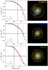 |
Fig. 1. Left-hand panels: Stellar surface density profile for three MW-like galaxies in the sample at z = 0. Right-hand panels: face-on projected stellar light images of the corresponding galaxies. The colours are based on the i-, g-, and u- band luminosities of stars. As is indicated in the right-hand panels, every row refers to a simulation suite. From top to bottom: AURIGA, HESTIA, and NIHAO with the corresponding stellar masses of 1.07 × 10¹⁰ M⊙, 1.56 × 10¹⁰ M⊙, and 2.15 × 10¹⁰ M⊙. Solid green and dash-dotted orange lines indicate the stellar half-mass and R1 radius, respectively. In the right-hand panels, a dashed green line is also incorporated to show the position of twice the stellar half-mass radius. |
4. Results
4.1. The R1 − M* relation
In this section, we present the R1–stellar mass relation for over 1000 galaxies with stellar masses between 4.9 × 10⁵ M⊙ and 1.9 × 10¹¹ M⊙, using AURIGA, HESTIA, and NIHAO (Figs. 2 and 3). We compare our R1 measurement with the stellar half-mass radius, R1/2, i.e. we divide the stellar mass range into 20 stellar mass bins and compute the median and 1-sigma scatter of R1 and R1/2 for the galaxies falling into each bin.
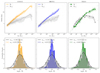 |
Fig. 2. Top panels: size–stellar mass relation for each of the simulation suites used in this work, where the stellar mass is measured within 20% of R200. The median values and 1σ scatter of the stellar half-mass radius in each stellar mass bin are shown by the grey lines and shaded regions, respectively. Likewise, the median values and 1σ scatter of galaxy size defined as R1 is shown for AURIGA (orange), HESTIA (blue), and NIHAO (green) by the lines and shaded regions, respectively. The sizes of individual galaxies are shown with dots (AURIGA), crosses (HESTIA), and squares (NIHAO), using the same colour criteria. Bottom panels: Normalised histograms of the distribution of galaxy sizes relative to the median ( |

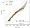 |
Fig. 3. R1 as a function of the stellar mass of galaxies, measured within 20% of R200, for different simulation suites, as is indicated in the legend. We show the median value of R1 measured within 20 stellar mass bins, equally spaced. Orange, blue, and green relations correspond to the AURIGA, HESTIA, and NIHAO samples. In addition, we also show in pink single FIRE-2 low-mass galaxies and the relation found by Dalla Vecchia & Trujillo in prep., using public data from EAGLE simulations in red. To compare with Trujillo et al. (2020), we add in grey their observational results as well as dashed lines, corresponding to locations in the place with a constant projected stellar mass density of (from top to bottom) 0.1, 1, 10, and 100 M⊙/pc2. |
The top panel of Fig. 2 shows the size–stellar mass relation for the three different simulations used in this work, in which we plot the 1-sigma scatter of the median values as a shaded area. Over the entire stellar mass range, the relation differs when using R1 compared to R1/2 as a proxy for the size of galaxies. For the AURIGA and HESTIA samples, the R1 − M⋆ relation becomes steeper and larger than R1/2 − M⋆ for galaxies with stellar masses larger than 107 M⊙. In contrast, for NIHAO, R1/2 exceeds R1 for M⋆ < 108 M⊙. This is because NIHAO simulations produce ‘cored’ dark matter haloes, which in turn give rise to ultra-diffuse galaxies at M⋆ ∼ 108 M⊙ that therefore have larger R1/2 than HESTIA or AURIGA galaxies at the same stellar mass (Di Cintio et al. 2014b,a; Tollet et al. 2016; Di Cintio et al. 2017).
The bottom panel of Fig. 2 shows the scatter within each of the simulation samples. Such a scatter is quantified as the standard deviation of a Gaussian distribution fitted to the residuals, defined as the difference between individual size measurements and their corresponding bin means. In the legend of each plot, we indicate that the numerical values of the global scatter for R1/2 is consistently larger than that of R1 at every stellar mass bin by factors of approximately 1.74 (AURIGA), 1.86 (HESTIA), and 1.34 (NIHAO), respectively. This is consistent with the observation results of Trujillo et al. (2020) when comparing the scatter of the size-stellar mass using R1 and Reff.
To assess the robustness of the R1–stellar mass relation found in the simulations, we plot, in Fig. 3, the relation for the AURIGA (orange), HESTIA (blue), and NIHAO (green) samples alongside one another. For comparison with observational data, we include dashed grey lines indicating constant projected stellar mass densities of 0.1, 1, 10 and 100 M⊙/pc2, from top to bottom, given by S⋆ = M⋆/πr22. We also show, with a dashed red line, the corresponding values for EAGLE galaxies (Dalla Vecchia & Trujillo in prep.), with stellar masses between 107.5 M⊙ and 1012 M⊙. Additionally, we extend our comparison with a sample of eight low-mass galaxies from the public FIRE-2 simulations (pink markers). Note that FIRE-2 galaxies were not included in the main analysis due to the limited number of galaxies available across the stellar mass range. However, it can be appreciated that both EAGLE and FIRE-2 follow the same trend as our simulation suites.
In agreement with Trujillo et al. (2020), the median stellar density within R1 lies above the 10 M⊙/pc2 line for galaxies with a stellar mass of M⋆ < 5 × 10⁸ M⊙, heading towards higher stellar mass densities for the most massive galaxies with M⋆ > 109 M⊙. Chamba et al. (2024) suggest that feedback and environmental processes may regulate galaxy sizes more rapidly in the low mass regime, compared to their massive counterpart, leading to a break in the size–stellar mass relation at ∼4 × 10⁸ M⊙, where it crosses the 10 M⊙/pc2 line. We note that the transition occurs at different stellar masses in NIHAO compared to AURIGA and HESTIA. This discrepancy may result from the different morphology of galaxies in each simulation sample: AURIGA and HESTIA massive galaxies tend to be disc-dominated spiral galaxies, while NIHAO’s massive galaxies predominantly exhibit an elliptical morphology (see Sec. 4.3 for more details). Observations suggest that the transition of R1 at the 10 M⊙/pc2 line likely reflects differences in the formation and accretion history of the most massive galaxies compared to lower-mass galaxies. Different predominant morphologies in each simulation could affect the stellar mass range in which this deviation occurs. All in all, galaxies with stellar masses from 107 to 1011 M⊙ follow a power law of R1 = M⋆β with β = 0.375, consistent with observations that find similar behaviour with β = 0.35 (Trujillo et al. 2020) and β = 0.377 (Hall et al. 2012). While different feedback schemes play a key role in defining the stellar half-mass radius (Crain et al. 2015), potentially explaining the discrepancies among simulations, R1 remains independent of the specific simulation suite and feedback scheme chosen. This suggests that R1 intrinsically captures the physics regulating star formation at the edges of galaxies.
4.2. Redshift evolution
In the previous sections, we demonstrated that R1 is a robust quantity for estimating galaxy size: it is consistent across the simulations suites probed. We now explore how R1 and its associated scatter evolve with redshift for all simulation suites.
In the left panel of Fig. 4, we present the median R1 values in each stellar mass bin over different redshifts: z ∼ 0.0, z ∼ 0.2, z ∼ 0.5, z ∼ 0.7 and z ∼ 1.0. Each redshift is coloured following the colour bar on the right, with the 1σ scatter for each redshift shown as a shaded region. The evolution of the normalisation and slope of the mean size-stellar mass relation does not change notably over redshift; however, the scatter at fixed stellar mass appears to decrease with increasing redshift. The right-hand panel shows the distribution of sizes at z ∼ 1.0, z ∼ 0.5, and z ∼ 0.0, which quantifies the decreasing scatter with increasing redshift. This evolutionary trend in the scatter may be linked to the cumulative effect of merger activity. In other words, galaxies at higher redshifts have experienced fewer mergers, leading to less diversity in galaxy sizes. This result aligns with previous studies using Reff, such as Nedkova et al. (2021) or Kawinwanichakij et al. (2021), which did not find significant changes in galaxy sizes across redshift. In contrast, Buitrago & Trujillo (2024) found that, using Redge as a proxy for the size, MW-like galaxies have doubled in size since z = 1. Although Chamba et al. (2020) found no significant differences when using Redge instead of R1, there is no guarantee that such a proxy based on MW-like galaxies should be able to characterize the radius to which in situ star formation takes places for all galaxies regardless of their evolution. However, due to the complexity of measuring Redge for non-massive galaxies, we opted to use R1. A more detailed study of size evolution across higher redshifts, based on a truncation in the stellar density profile, is deferred to future research.
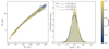 |
Fig. 4. R1 as a function of galaxy stellar mass over redshift for all the galaxies in our sample, where the stellar mass is measured within 20% of R200. The left-hand panel shows the median value of the galaxy size, measured using the R1 criteria, for all simulations. Each colour represents a different redshift, from z = 0 (in blue) to z = 1 (in yellow). The median value of the size has been measured within 20 stellar mass bins in each case. We also show the 1σ error as shaded regions. The right-hand panel shows a normalised histogram of the scatter between each singular size value and its corresponding bin value, |

In addition to studying the evolution of the size–stellar mass relation, simulations provide the opportunity to examine the evolution of the sizes of individual galaxies. A question that arises is whether the galaxies evolve along this relation. To address this, we selected galaxies at z = 0 from each simulation sample in four stellar mass ranges within a bin of ±0.5 dex: 107, 108, 109, and 1010 M⊙. We tracked these galaxies back in time up to z = 13, using five increasing z. Fig. 5 illustrates the median evolution for each stellar mass range and simulation suite. Generally, galaxies evolve along the size-stellar mass relation, regardless of the stellar mass range and simulation suite. An exception is found in the NIHAO sample, where galaxies that lie in the size–stellar mass relation at z = 1 for the stellar mass bin ∼109 M⊙ ended with larger sizes at present-day redshift compared to galaxies in other simulation suites. Note that, even when present-day galaxies have larger sizes than the average, their progenitors still lie in the R1 relation at earlier redshifts. The discrepancy in NIHAO galaxies for this stellar mass range is explained by repeated SNe-driven gas outflows, which build up larger galaxies with time, particularly in the stellar mass range M⋆ ∼ 108 − 9 M⊙ (Di Cintio et al. 2014b,a, 2017; Pontzen & Governato 2012). The initial selection and morphology of NIHAO galaxies (see Fig. 3) indicate that they tend to be larger than those in AURIGA and HESTIA samples for stellar masses between 108 and 109 M⊙. Another exception is the evolution in the low mass range. While the stellar mass in AURIGA and HESTIA galaxies seems to evolve continuously and monotonically along the relation over the four stellar mass ranges, the NIHAO galaxies exhibit a different evolution for dwarfs: galaxies with 107 M⊙ stellar masses evolve very little in stellar mass or size, and galaxies in the ∼108 M⊙ stellar mass range at z = 0 are larger at higher redshifts compared to those from AURIGA and HESTIA. Different feedback schemes could be the reason for evolution discrepancies between the simulation samples. This may be particularly true in the low mass regime, where the modelling and implementation of a relatively low number of feedback events in relatively shallow dark matter halo potentials can significantly shape galaxy properties. Overall, we demonstrate that galaxies evolve along the R1 − M⋆ relation at various z, despite the specific stellar mass or simulation used.
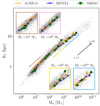 |
Fig. 5. Evolution of R1 as a function of galaxy stellar mass, measured within 20% of R200, over four different stellar mass ranges. For each simulation suite, we selected z = 0 galaxies at 107, 108, 109, and 1010 M⊙, within a bin of ±0.5 dex, and tracked their size-evolution over redshift up to z = 1, using five increasing z, from left to right. Each of the stellar mass ranges selected is indicated and zoomed in with brown, pink, yellow, and blue regions, respectively. The median value of the size and the stellar mass has been measured for each of the redshifts. Orange dots represent the size evolution of the AURIGA suite, while blue crosses and green squares indicate the HESTIA and NIHAO samples, respectively. The whole sample at z = 0, regardless of the simulation suite, is also shown as grey dots. |
4.3. Morphology dependence
We have shown that using R1 to measure the global size-stellar mass relation of galaxies decreases the scatter by about twice as much as using R1/2. We now check whether this is also the case for different morphologies. We examined the R1–stellar mass relation by categorising sample galaxies into two groups, regardless of the simulation used: rotationally supported and non-rotationally supported, i.e. dispersionally supported. We classified galaxies as rotationally supported following the criteria from Correa et al. (2017), in which galaxies with κco > 0.4 are distinguished as spiral galaxies and ones with κco < 0.4 as ellipticals. Here, κco is the fraction of the kinetic energy of the galaxy invested in ordered co-rotation (see Sales et al. (2010) and Correa et al. (2017) for more details). Fig. 6 illustrates the correlation between larger sizes and higher co-rotational velocities, showing that spiral galaxies tend to have larger R1 sizes than elliptical galaxies at a fixed stellar mass, for a stellar mass larger than ∼4 × 10⁷ M⊙. This finding agrees with observational results from Trujillo et al. (2020). Below this stellar mass, we can appreciate a change in behaviour, in which the trend reverses. Dispersion-supported galaxies host larger sizes than rotational galaxies at lower stellar masses. However, this could be due to statistical limitations – since the sample of rotational galaxies at those stellar masses may not be representative in this case (see top panel of Fig. 6) – dispersion-dominated dwarfs tend to be cored galaxies and might have larger sizes than the more discy ones. It is important to note that in our sample elliptical and spiral galaxies coexist within the same stellar mass range. As is discussed in Section 4.1, observed galaxies from Trujillo et al. (2020) reach higher stellar masses, where the distinction between ellipticals and spirals becomes more pronounced, with limited overlap between the two morphologies. While we cannot replicate galaxies in this most massive region, we still observe differences in the slope between elliptical and spiral morphologies, consistent with their findings in the stellar mass range where both morphologies coexist.
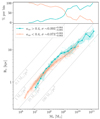 |
Fig. 6. R1 as a function of galaxy stellar mass, measured within 20% of R200, for all galaxies in the three simulations of our sample. Each of them is characterised as rotational (shown in blue) or dispersion (shown in pink) supported, following the criteria of Sales et al. (2010) and Correa et al. (2017). The median size value has been measured across 20 stellar mass bins in each case. We also show as shaded regions the 1σ error for both classifications. The top panel represents the percentage of galaxies in each morphology per bin, following the same colour code as the main panel. The global FWHM of the relation was found by fitting a Gaussian distribution, and it is indicated in the legend as σ, whose errors were computed via bootstrapping. |
For both cases, we have measured the 1σ scatter, finding a smaller scatter, σ ∼ 0.073 ± 0.003 dex, in those galaxies supported by dispersion. This result may seem in contradiction with previous discussions, primarily since R1 was designed for MW-like galaxies. However, the scatter has been measured across the entire stellar mass range – from 107 M⊙ to 1011 M⊙ for rotation-supported galaxies and 106 − 1010 M⊙ for dispersion-supported galaxies. Thus, the scatter found for disk galaxies cannot be interpreted as the general behaviour of MW-like galaxies.
Fig. 7 shows the general co-rotational behaviour concerning the galaxy’s stellar mass for each simulation suite. In the low-mass regime, all galaxies, regardless of the simulation, tend to exhibit elliptical morphologies, with the median co-rotational value remaining below 0.4, until the galaxies reach a stellar mass of about 109 M⊙. For more massive galaxies, we can appreciate a large difference between AURIGA and HESTIA galaxies and NIHAO galaxies. The reason for this difference can be ascribed to the different selection criteria originally adopted in constructing the three simulated samples. While HESTIA and AURIGA galaxies are popularly used for the study of MW-like galaxies and their environment, NIHAO galaxies do not target any particular morphological type. However, NIHAO tends to harbour a high population of elliptical galaxies. An exception to this trend occurs in those galaxies with a stellar mass range between 108 and 109 M⊙, where the NIHAO sample has a greater number of spirals than their counterparts in the other simulations. This behaviour is also reflected in Figs. 3 and 5, where higher values of R1 are found for NIHAO galaxies within this stellar mass regime.
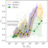 |
Fig. 7. Fraction of kinetic energy invested in ordered co-rotation versus stellar mass for each simulation suite. We show the median value of the co-rotation fraction measured within 20 stellar mass bins. Orange, blue, and green relations correspond to the AURIGA, HESTIA, and NIHAO samples. We also show as orange, blue, and green shaded regions the 1σ scatter for AURIGA, HESTIA, and NIHAO, respectively. Galaxies above the horizontal dashed line are considered rotationally supported and vice versa (see Sales et al. 2010 and Correa et al. 2017 for more details about the selection criteria). |
4.4. The connection with halo properties
In the previous section, we showed that the scatter in R1 is generally a factor of almost two smaller than that found in R1/2. We now explore R1 as an alternative metric to R1/2 when investigating the connection between galaxies and their host dark matter halos.
The scatter of the SHMR is an interesting quantity because it reflects the efficiency of galaxy formation at a fixed halo mass: galaxies with higher stellar masses have been more efficient in forming stars than their less massive counterparts. Thus, this scatter is expected to be linked to the baryonic cycle of galaxies; however, how it connects to galaxy properties remains a matter of debate (Wechsler & Tinker 2018). With uncertainties in halo mass estimations being one of the main challenges in exploring this issue observationally, Scholz-Díaz et al. (2024) introduce the STMR as a direct observational alternative to studying the galaxy-halo connection, with total dynamical masses measured within 3Reff. They find that galaxy properties exhibit similar trends across the scatter of both the SHMR and the STMR, with total dynamical masses correlating with halo masses at a fixed stellar mass. Based on this, they argue that total dynamical mass measured within 3Reff serves as a proxy for halo mass and that the scatter of the STMR can be used as an alternative to that of the SHMR. In this section, we investigate whether total masses measured within R1 are able to trace their halo masses. If so, R1 could serve not only as a reliable size measure but also as a direct method of studying the connection between galaxies and their halo properties. Analogous to the work of Dalla Vecchia & Trujillo in prep. – who explore the R1 − R200 for EAGLE galaxies, finding a notable small scatter that can be used to infer properties of their host halos – we measure the total mass as contained within R1, and later compare it with the observational results from Scholz-Díaz et al. (2024), who computed the total dynamical mass following 3D Jeans equations (see Zhu et al. 2023 for more details).
Fig. 8 shows both the SHMR (top panel) and the STMR inside R1 and 3R1/2 (bottom panel) using coloured and grey markers, analogous to the STMR measured within 3Reff from Scholz-Díaz et al. (2024). Note that Reff in observational studies is derived from a photometric band that is not always available in our sample. For this reason, we use R1/2 for comparison, as it provides a more consistent measurement across different simulations. In the top panel, the purple, dark, and magenta curves represent semi-empirical relations from Moster et al. (2013), Guo et al. (2010), and Girelli et al. (2020), respectively. While NIHAO galaxies follow the Moster et al. (2013) semi-empirical relation, AURIGA and HESTIA are placed above this relation for the M200 < 1011 M⊙ range. However, note that below this halo mass a large uncertainty exists in the predicted relation (see Girelli et al. (2020) for more details). Whether a simulation matches the abundance matching relations depends significantly on how feedback mechanisms are implemented. For example, while EAGLE is calibrated to match the abundance matching relation across their high mass ranges (see Fig. 8. of Schaye et al. (2015)), the NIHAO sample used in this paper does not include active galactic nucleus (AGN) feedback (see Blank et al. (2019) for AGN implementation in NIHAO) and yet reproduces the SHMR across a large galaxy mass range. In contrast, AURIGA and HESTIA, though not explicitly calibrated to match the abundance matching relation, incorporate both AGN and SN feedback.
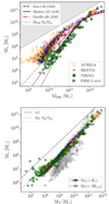 |
Fig. 8. Upper panel: stellar-to-halo mass relation (SHMR) for each of the simulation suites. In solid purple, the abundance matching relation from Moster et al. (2013) is shown with a 0.2 dex scatter. The dashed dark and dash-dotted magenta lines represent estimates by Guo et al. (2010) and Girelli et al. (2020), respectively. Thick lines correspond to the range where the abundance matching relations are constrained by observations, while the thin lines are extrapolations. Bottom panel: stellar mass versus total mass within R1 (STMR), where the stellar mass is measured within 20% of R200. The dashed line represents the 1:1 relation. The universal baryon fraction is shown with a dotted line in both cases. Empty orange dots, blue crosses, green squares, and pink triangles represent the AURIGA, HESTIA, NIHAO, and FIRE-2 samples, respectively. For comparison, we also show in grey squares, dots, and crosses the STMR within 3R1/2. |
Given the robustness of the R1–stellar mass relation across the different simulation suites demonstrated in the previous section, we can expect a stronger correlation between the total mass within R1 and the stellar mass (STMR) compared to the SHMR. The bottom panel of Fig. 8 shows the former for each simulation suite, with notably reduced scatter at the low-mass end compared to the SHMR. Additionally, the STMR within 3R1/2 is shown in grey. In both STMR cases, the scatter for each simulation suite has been measured (not shown), revealing a systematic reduction when using R1. The median scatter of STMR within R1 is found to be σR1 ∼ 0.15 ± 0.01 dex, whereas the scatter measured within 3R1/2 is σ3R1/2 ∼ 0.28 ± 0.02 dex. Alongside the STMR relation, we also show the 1:1 line and the universal baryon fraction with dashed and dotted lines, respectively. The fact that galaxies closely follow the universal baryon fraction line can be explained by R1 corresponding to the radius where the gas density required for SF reaches a minimum. Under this assumption, all stellar mass is enclosed within R1. Galaxies with stellar mass below 109 M⊙ fall below the universal baryon fraction relation, while MW-like galaxies seem to match it. We found several outliers below 108 M⊙ for the NIHAO sample, with stellar masses larger than expected for a fixed total mass, even surpassing the 1:1 line. For galaxies above this line, we inspected the stellar surface density profile (not shown here). In each of these galaxies, the maximum values in their stellar density barely reach the Σ⋆ = 1 M⊙/pc2 threshold, leading to R1 values not capable of enclosing the whole galaxy. This threshold is defined for MW-like galaxies and differs for dwarfs or elliptical galaxies (see Trujillo et al. 2020 and references therein for more details); thus, low-mass galaxies whose sizes cannot be explained by using R1 are to be expected. However, note that for galaxies for which the maximum value of the stellar surface density profile is well above the density threshold, we can still recover the expected size-stellar mass relation.
For a visual inspection, we extend our results with eight low-mass FIRE-2 galaxies, shown with single pink markers, which lie in the same space as other simulation suites. In addition, we present in Appendix A the total cumulative mass versus radius for four different stellar masses: ∼1010, 109, 108, and 107 M⊙. While the cumulative total mass distribution evolves differently across the entire radius depending on the simulation suite used, the median profiles of each sample consistently intersect at ∼R1, regardless of the stellar mass range. This implies that AURIGA, HESTIA, and NIHAO galaxies tend to have the same amount of total mass at the R1 range (shown in grey), diverging again at larger radii. Galaxies from the FIRE-2 sample that fall within the corresponding stellar mass ranges are also shown, intersecting with the other samples at R1 as well. However, since only a few FIRE-2 galaxies fall into this range, we may not be able to interpret them as a systematic trend.
Although the focus of this work is not on the baryonic processes that influence the scatter in the SHMR, examining the halo mass derived from the total mass within R1 could provide valuable insights into the relationship between these processes. To assess whether the total mass within R1 accurately traces the halo mass – and thus whether the scatter in the STMR could serve as an alternative to the SHMR – we conduct an analysis similar to that of Scholz-Díaz et al. (2024) in Appendix B. It is important to note, however, that we assume R1 fully encompasses the stellar mass of galaxies, independent of their morphology. A more detailed exploration of the baryonic processes influencing halo properties will be addressed in future work.
5. Conclusions
The sizes of galaxies have been a subject of extensive study over the past few decades, as they are essential in our understanding of how galaxies form and evolve. However, it is only in recent years that observational studies have begun to explore the borders of galaxies using physically motivated definitions. Specifically, these studies have employed the location of the gas density threshold for star formation as a natural size indicator (Trujillo et al. 2020; Chamba et al. 2022; Buitrago & Trujillo 2024). The radius R1, which serves as a proxy for this critical gas density threshold (Martínez-Lombilla et al. 2019), has been shown observationally to reduce the scatter in the size-stellar mass relation of galaxies. In this paper, we aim to assess the reliability of this new definition across different state-of-the-art hydrodynamical simulation suites. The key findings of our work are summarised as follows:
-
The size–stellar mass relation obtained using R1 shows a systematic reduction in scatter by a factor of ∼2 dex compared to the relation defined by R1/2, for all simulation suites (Figs. 2 and 3). These results are in agreement with observations of Trujillo et al. (2020), including the general trend, whereby massive galaxies above 109 M⊙ begin to exhibit a shallower size-stellar mass slope, as is shown in Fig. 3.
-
We study the evolution of the size–stellar mass relation up to z ∼ 1 and find that the slope and normalisation of the relation are redshift-independent, and that the scatter decreases with increasing redshift (Fig. 4). We find that most simulated galaxies have evolutionary tracks that lie along the median R1–stellar mass relation.
-
Regarding morphology, we divided the whole sample into rotational and dispersion-supported galaxies, based on the criteria of Correa et al. (2017) (Fig. 6). For stellar masses above 107 M⊙, rotationally supported galaxies generally exhibit larger sizes compared to those that are dispersion-supported, indicating that the new size definition, R1, is correlated with the morphology of galaxies. Below 107 M⊙, we find larger sizes in galaxies supported by dispersion. However, it is important to note that, in this lower mass range, the number of rotationally supported galaxies is low.
-
Although each simulation suite is strongly influenced by the feedback models implemented, the use of R1, not only as a measure of galaxy size but also as a means to study the connection with halo properties, yields a stronger correlation between stellar mass and total mass enclosed within R1 compared to the traditionally used SHMR (Fig. 8). For galaxies with stellar masses above 109 M⊙, we observe a consistent correlation in the scatter between SHMR and STMR (Fig. B.1), which is also consistent with properties that correlate to the SHMR scatter, similar to the findings of Scholz-Díaz et al. (2024) using 3Reff. This suggests that R1 could also serve as a viable observational tracer of the halo mass. Those baryonic processes that influence the galaxy at fixed stellar mass, shaping the scatter of SHMR, can also be inferred by studying the scatter in the STMR.
We caution the reader that the stellar and halo mass ranges explored in this work are limited at the upper end by MW-size galaxies and do not cover the most massive range. In the future, extending the sample to include larger galaxies will provide valuable insights into identifying the slope change between elliptical and MW-like galaxies, discussed throughout the paper. Additionally, while we used R1 as a size indicator instead of Redge, it is important to note that although both quantities are observed to be very similar at z ∼ 0, their differences may become significant at higher redshifts. A thorough investigation of Redge will be essential for understanding changes in galaxy sizes and their evolution over time.
These simulations correspond to the Original/4 set of publicly available simulations described in Grand et al. (2024).
Note that in this paper we plot lines of constant M⋆/πr2, which is a factor of π different from the lines plotted in Trujillo et al. (2020).
We select those galaxies that can be tracked up to z = 1 by using the most massive progenitor at each snapshot defined by AHF’s merger tree.
We use the halo concentration values from AHF, which numerically computes the concentration using Eq. 9 from Prada et al. (2012).
Acknowledgments
The authors sincerely thank Dr. Ignacio Trujillo and Dr. Laura V. Sales for their valuable insights. E. Arjona-Gálvez acknowledges support from the Agencia Espacial de Investigación del Ministerio de Ciencia e Innovación (AEI-MICIN) and the European Social Fund (ESF+) through a FPI grant PRE2020-096361. SCB acknowledges financial support from the Spanish Ministry of Science and Innovation (MICINN) for PID2021-128131NB-I00 (CoBEARD) and CNS2022-135482 projects. RG acknowledges financial support from an STFC Ernest Rutherford Fellowship (ST/W003643/1). A. Di Cintio thanks the University of La Laguna (ULL) for financial support through a “Noveles Investigadores” grant, and the Ministry of Science and Innovation for additional funding from the EU Next Generation Funds under the 2023 Consolidación Investigadora program (grant code CNS2023-144669). CDV also acknowledges support from MICIU in the early stages of development of this work through grants RYC-2015-18078 and PGC2018-094975-C22. JAB is grateful for partial financial support from NSF-CAREER-1945310 and NSF-AST-2107993 grants and data storage resources of the HPCC, which were funded by grants from NSF (MRI-2215705, MRI-1429826) and NIH (1S10OD016290-01A1). NIL acknowledges funding by the European Union’s Horizon Europe research and innovation program (EXCOSM, grant No. 101159513). AK is supported by the Ministerio de Ciencia e Innovación (MICINN) under research grant PID2021-122603NB-C21 and further thanks Teenage Fanclub for thirteen. This research made use of the LaPalma HPC cluster, under project can43, PI A. Di Cintio, as well as the High-Performance Computers located at the Instituto de Astrofísica de Canarias. The authors thankfully acknowledge the technical expertise and assistance provided by the IAC (Servicios Informáticos Específicos, SIE) and the Spanish Supercomputing Network (Red Española de Supercomputación, RES).
References
- Blank, M., Macciò, A. V., Dutton, A. A., & Obreja, A. 2019, MNRAS, 487, 5476 [NASA ADS] [CrossRef] [Google Scholar]
- Buitrago, F., & Trujillo, I. 2024, A&A, 682, A110 [NASA ADS] [CrossRef] [EDP Sciences] [Google Scholar]
- Carlesi, E., Sorce, J. G., Hoffman, Y., et al. 2016, MNRAS, 458, 900 [NASA ADS] [CrossRef] [Google Scholar]
- Chamba, N. 2020, Res. Notes. Am. Astron. Soc., 4, 117 [Google Scholar]
- Chamba, N., Trujillo, I., & Knapen, J. H. 2020, A&A, 633, L3 [NASA ADS] [CrossRef] [EDP Sciences] [Google Scholar]
- Chamba, N., Trujillo, I., & Knapen, J. H. 2022, A&A, 667, A87 [NASA ADS] [CrossRef] [EDP Sciences] [Google Scholar]
- Chamba, N., Marcum, P. M., Saintonge, A., et al. 2024, ApJ, 974, 247 [Google Scholar]
- Correa, C. A., Schaye, J., Clauwens, B., et al. 2017, MNRAS, 472, L45 [Google Scholar]
- Crain, R. A., Schaye, J., Bower, R. G., et al. 2015, MNRAS, 450, 1937 [NASA ADS] [CrossRef] [Google Scholar]
- de Vaucouleurs, G. 1948, Ann. d’Astrophys., 11, 247 [Google Scholar]
- Di Cintio, A., Brook, C. B., Dutton, A. A., et al. 2014a, MNRAS, 441, 2986 [Google Scholar]
- Di Cintio, A., Brook, C. B., Macciò, A. V., et al. 2014b, MNRAS, 437, 415 [Google Scholar]
- Di Cintio, A., Brook, C. B., Dutton, A. A., et al. 2017, MNRAS, 466, L1 [NASA ADS] [CrossRef] [Google Scholar]
- Fritz, T. K., Di Cintio, A., Battaglia, G., Brook, C., & Taibi, S. 2020, MNRAS, 494, 5178 [Google Scholar]
- Girelli, G., Pozzetti, L., Bolzonella, M., et al. 2020, A&A, 634, A135 [NASA ADS] [CrossRef] [EDP Sciences] [Google Scholar]
- Gottloeber, S., Hoffman, Y., & Yepes, G. 2010, ArXiv e-prints [arXiv:1005.2687] [Google Scholar]
- Graham, A. W. 2019, PASA, 36, e035 [NASA ADS] [CrossRef] [Google Scholar]
- Grand, R. J. J., Gómez, F. A., Marinacci, F., et al. 2017, MNRAS, stx071, [Google Scholar]
- Grand, R. J. J., Fragkoudi, F., Gómez, F. A., et al. 2024, MNRAS, 532, 1814 [NASA ADS] [CrossRef] [Google Scholar]
- Guo, Q., White, S., Li, C., & Boylan-Kolchin, M. 2010, MNRAS, 404, 1111 [NASA ADS] [Google Scholar]
- Hall, M., Courteau, S., Dutton, A. A., McDonald, M., & Zhu, Y. 2012, MNRAS, 425, 2741 [Google Scholar]
- Holmberg, E. 1958, Meddelanden fran Lunds Astronomiska Observatorium Serie II, 136, 1 [Google Scholar]
- Kawinwanichakij, L., Silverman, J. D., Ding, X., et al. 2021, ApJ, 921, 38 [NASA ADS] [CrossRef] [Google Scholar]
- Knollmann, S. R., & Knebe, A. 2009, ApJS, 182, 608 [Google Scholar]
- Kron, R. G. 1980, ApJS, 43, 305 [Google Scholar]
- Libeskind, N. I., Carlesi, E., Grand, R. J. J., et al. 2020, MNRAS, 498, 2968 [NASA ADS] [CrossRef] [Google Scholar]
- Mandelbaum, R., Blazek, J., Chisari, N. E., et al. 2019, BAAS, 51, 363 [NASA ADS] [Google Scholar]
- Martínez-Lombilla, C., Trujillo, I., & Knapen, J. H. 2019, MNRAS, 483, 664 [CrossRef] [Google Scholar]
- Matthee, J., Schaye, J., Crain, R. A., et al. 2017, MNRAS, 465, 2381 [NASA ADS] [CrossRef] [Google Scholar]
- Mo, H. J., Mao, S., & White, S. D. M. 1998, MNRAS, 295, 319 [Google Scholar]
- Mo, H., van den Bosch, F. C., & White, S. 2010, Galaxy Formation and Evolution (Cambridge: Cambridge University Press) [Google Scholar]
- More, S., van den Bosch, F. C., Cacciato, M., et al. 2011, MNRAS, 410, 210 [Google Scholar]
- Moster, B. P., Naab, T., & White, S. D. M. 2013, MNRAS, 428, 3121 [Google Scholar]
- Nair, P., van den Bergh, S., & Abraham, R. G. 2011, ApJ, 734, L31 [NASA ADS] [CrossRef] [Google Scholar]
- Nedkova, K. V., Häußler, B., Marchesini, D., et al. 2021, MNRAS, 506, 928 [NASA ADS] [CrossRef] [Google Scholar]
- Ou, X., Eilers, A.-C., Necib, L., & Frebel, A. 2024, MNRAS, 528, 693 [NASA ADS] [CrossRef] [Google Scholar]
- Pakmor, R., Springel, V., Bauer, A., et al. 2016, MNRAS, 455, 1134 [Google Scholar]
- Petrosian, V. 1976, ApJ, 210, L53 [NASA ADS] [CrossRef] [Google Scholar]
- Pillepich, A., Springel, V., Nelson, D., et al. 2018, MNRAS, 473, 4077 [Google Scholar]
- Planck Collaboration XVI 2014, A&A, 571, A16 [NASA ADS] [CrossRef] [EDP Sciences] [Google Scholar]
- Pontzen, A., & Governato, F. 2012, MNRAS, 421, 3464 [NASA ADS] [CrossRef] [Google Scholar]
- Pontzen, A., Roškar, R., Stinson, G., & Woods, R. 2013, Astrophysics Source Code Library [record ascl:1305.002] [Google Scholar]
- Prada, F., Klypin, A. A., Cuesta, A. J., Betancort-Rijo, J. E., & Primack, J. 2012, MNRAS, 423, 3018 [NASA ADS] [CrossRef] [Google Scholar]
- Redman, R. O. 1936, MNRAS, 96, 588 [CrossRef] [Google Scholar]
- Sales, L. V., Navarro, J. F., Schaye, J., et al. 2010, MNRAS, 409, 1541 [Google Scholar]
- Sánchez Almeida, J. 2020, MNRAS, 495, 78 [Google Scholar]
- Schaye, J. 2004, ApJ, 609, 667 [NASA ADS] [CrossRef] [Google Scholar]
- Schaye, J., Crain, R. A., Bower, R. G., et al. 2015, MNRAS, 446, 521 [Google Scholar]
- Scholz-Díaz, L., Martín-Navarro, I., Falcón-Barroso, J., Lyubenova, M., & van de Ven, G. 2024, Nature, 8, 648 [Google Scholar]
- Sersic, J. L. 1968, Atlas de Galaxias Australes (Cordoba: Observatorio Astronomico) [Google Scholar]
- Springel, V. 2010, MNRAS, 401, 791 [Google Scholar]
- Tollet, E., Macciò, A. V., Dutton, A. A., et al. 2016, MNRAS, 456, 3542 [CrossRef] [Google Scholar]
- Trujillo, I., Graham, A. W., & Caon, N. 2001, MNRAS, 326, 869 [Google Scholar]
- Trujillo, I., Chamba, N., & Knapen, J. H. 2020, MNRAS, 493, 87 [NASA ADS] [CrossRef] [Google Scholar]
- Tully, R. B., Courtois, H. M., Dolphin, A. E., et al. 2013, AJ, 146, 86 [NASA ADS] [CrossRef] [Google Scholar]
- van der Wel, A., Franx, M., van Dokkum, P. G., et al. 2014, ApJ, 788, 28 [Google Scholar]
- Wadsley, J. W., Keller, B. W., & Quinn, T. R. 2017, MNRAS, 471, 2357 [NASA ADS] [CrossRef] [Google Scholar]
- Wang, L., Dutton, A. A., Stinson, G. S., et al. 2015, MNRAS, 454, 83 [NASA ADS] [CrossRef] [Google Scholar]
- Wechsler, R. H., & Tinker, J. L. 2018, ARA&A, 56, 435 [NASA ADS] [CrossRef] [Google Scholar]
- Zhu, K., Lu, S., Cappellari, M., et al. 2023, MNRAS, 522, 6326 [NASA ADS] [CrossRef] [Google Scholar]
- Zu, Y., Shan, H., Zhang, J., et al. 2021, MNRAS, 505, 5117 [CrossRef] [Google Scholar]
Appendix A: Cumulative total mass profiles
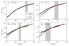 |
Fig. A.1. Cumulative total mass versus radius across four stellar mass ranges. Each simulation suite is coloured according to the colour code of the simulation suite. For each simulation suite, we select z = 0 galaxies at 1010, 109, 108 and 107 M⊙ (from top left to bottom right), within a bin of ±0.5dex. The median cumulative total mass profile is shown with a solid thick line in orange, blue, green and pink for the AURIGA, HESTIA, NIHAO and FIRE-2 galaxies, respectively. The vertical grey region covers all the R1 values found for each stellar mass range. |
Appendix B: Total mass versus halo mass
We conduct an analogous analysis from Scholz-Díaz et al. (2024) (see their Fig. Extended Data Fig. 2 and Methods section) to investigate whether the scatter of the STMR can be used as an alternative metric to the SHMR. Fig. B.1 reflects the residuals of M200 and MT for galaxies above M⋆ > 109 M⊙. We choose this stellar mass range to exclude low-mass dwarf galaxies for which the scatter in stellar mass (at fixed M200) is heavily influenced by baryonic physics. The scatter has been measured by assuming both SHMR and STMR for galaxies above a stellar mass of 109 M⊙ follow a linear distribution.
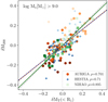 |
Fig. B.1. Halo mass versus total mass within R1. We show the δM200 and δMT(< R1) residuals from the log M200 − log M⋆ versus log MT(< R1) − log M⋆ relations, for galaxies with M⋆ > 109 M⊙. AURIGA, HESTIA and NIHAO galaxies are shown with orange dots, blue crosses and green squares. Every galaxy is coloured by the concentration of its halo, with darker colours referring to higher concentration and vice versa. Every suite is upper and lower limited by a halo concentration value of 40 and 7, respectively. Best-fitting is shown following the same colour code used for each simulation suite, along with their Spearman rank correlation coefficients. We also show, within dashed grey, the 1:1 line for reference. |
The positive correlation indicated by the Spearman rank coefficients means that, at fixed stellar mass, galaxies with higher total masses within R1, MT, tend to have larger M200. To highlight the importance of the correlation between STMR’s and SHMR’s scatters, we have coloured every galaxy by its halo concentration4, one of the properties that correlate with the SHMR scatter (Matthee et al. 2017; Zu et al. 2021). Dark colours refer to higher concentration values and vice versa. At fixed stellar mass, halos with positive scatter values, i.e. larger halo and total masses, have a lower concentration than those with smaller halo and/or total masses. Such behaviour indicates that those properties responsible for the scatter in the SHMR could be inferred by inspecting their scatter in STMR. This result aligns with the observational findings of Scholz-Díaz et al. (2024), who used the total dynamical mass within 3Reff to investigate several baryonic processes that affect the STMR scatter.
All Tables
Resolution parameters and number of total galaxies retained in the three different simulation suites at z = 0.
All Figures
|
Fig. 1. Left-hand panels: Stellar surface density profile for three MW-like galaxies in the sample at z = 0. Right-hand panels: face-on projected stellar light images of the corresponding galaxies. The colours are based on the i-, g-, and u- band luminosities of stars. As is indicated in the right-hand panels, every row refers to a simulation suite. From top to bottom: AURIGA, HESTIA, and NIHAO with the corresponding stellar masses of 1.07 × 10¹⁰ M⊙, 1.56 × 10¹⁰ M⊙, and 2.15 × 10¹⁰ M⊙. Solid green and dash-dotted orange lines indicate the stellar half-mass and R1 radius, respectively. In the right-hand panels, a dashed green line is also incorporated to show the position of twice the stellar half-mass radius. |
| In the text | |
|
Fig. 2. Top panels: size–stellar mass relation for each of the simulation suites used in this work, where the stellar mass is measured within 20% of R200. The median values and 1σ scatter of the stellar half-mass radius in each stellar mass bin are shown by the grey lines and shaded regions, respectively. Likewise, the median values and 1σ scatter of galaxy size defined as R1 is shown for AURIGA (orange), HESTIA (blue), and NIHAO (green) by the lines and shaded regions, respectively. The sizes of individual galaxies are shown with dots (AURIGA), crosses (HESTIA), and squares (NIHAO), using the same colour criteria. Bottom panels: Normalised histograms of the distribution of galaxy sizes relative to the median ( |
| In the text | |
|
Fig. 3. R1 as a function of the stellar mass of galaxies, measured within 20% of R200, for different simulation suites, as is indicated in the legend. We show the median value of R1 measured within 20 stellar mass bins, equally spaced. Orange, blue, and green relations correspond to the AURIGA, HESTIA, and NIHAO samples. In addition, we also show in pink single FIRE-2 low-mass galaxies and the relation found by Dalla Vecchia & Trujillo in prep., using public data from EAGLE simulations in red. To compare with Trujillo et al. (2020), we add in grey their observational results as well as dashed lines, corresponding to locations in the place with a constant projected stellar mass density of (from top to bottom) 0.1, 1, 10, and 100 M⊙/pc2. |
| In the text | |
|
Fig. 4. R1 as a function of galaxy stellar mass over redshift for all the galaxies in our sample, where the stellar mass is measured within 20% of R200. The left-hand panel shows the median value of the galaxy size, measured using the R1 criteria, for all simulations. Each colour represents a different redshift, from z = 0 (in blue) to z = 1 (in yellow). The median value of the size has been measured within 20 stellar mass bins in each case. We also show the 1σ error as shaded regions. The right-hand panel shows a normalised histogram of the scatter between each singular size value and its corresponding bin value, |
| In the text | |
|
Fig. 5. Evolution of R1 as a function of galaxy stellar mass, measured within 20% of R200, over four different stellar mass ranges. For each simulation suite, we selected z = 0 galaxies at 107, 108, 109, and 1010 M⊙, within a bin of ±0.5 dex, and tracked their size-evolution over redshift up to z = 1, using five increasing z, from left to right. Each of the stellar mass ranges selected is indicated and zoomed in with brown, pink, yellow, and blue regions, respectively. The median value of the size and the stellar mass has been measured for each of the redshifts. Orange dots represent the size evolution of the AURIGA suite, while blue crosses and green squares indicate the HESTIA and NIHAO samples, respectively. The whole sample at z = 0, regardless of the simulation suite, is also shown as grey dots. |
| In the text | |
|
Fig. 6. R1 as a function of galaxy stellar mass, measured within 20% of R200, for all galaxies in the three simulations of our sample. Each of them is characterised as rotational (shown in blue) or dispersion (shown in pink) supported, following the criteria of Sales et al. (2010) and Correa et al. (2017). The median size value has been measured across 20 stellar mass bins in each case. We also show as shaded regions the 1σ error for both classifications. The top panel represents the percentage of galaxies in each morphology per bin, following the same colour code as the main panel. The global FWHM of the relation was found by fitting a Gaussian distribution, and it is indicated in the legend as σ, whose errors were computed via bootstrapping. |
| In the text | |
|
Fig. 7. Fraction of kinetic energy invested in ordered co-rotation versus stellar mass for each simulation suite. We show the median value of the co-rotation fraction measured within 20 stellar mass bins. Orange, blue, and green relations correspond to the AURIGA, HESTIA, and NIHAO samples. We also show as orange, blue, and green shaded regions the 1σ scatter for AURIGA, HESTIA, and NIHAO, respectively. Galaxies above the horizontal dashed line are considered rotationally supported and vice versa (see Sales et al. 2010 and Correa et al. 2017 for more details about the selection criteria). |
| In the text | |
|
Fig. 8. Upper panel: stellar-to-halo mass relation (SHMR) for each of the simulation suites. In solid purple, the abundance matching relation from Moster et al. (2013) is shown with a 0.2 dex scatter. The dashed dark and dash-dotted magenta lines represent estimates by Guo et al. (2010) and Girelli et al. (2020), respectively. Thick lines correspond to the range where the abundance matching relations are constrained by observations, while the thin lines are extrapolations. Bottom panel: stellar mass versus total mass within R1 (STMR), where the stellar mass is measured within 20% of R200. The dashed line represents the 1:1 relation. The universal baryon fraction is shown with a dotted line in both cases. Empty orange dots, blue crosses, green squares, and pink triangles represent the AURIGA, HESTIA, NIHAO, and FIRE-2 samples, respectively. For comparison, we also show in grey squares, dots, and crosses the STMR within 3R1/2. |
| In the text | |
|
Fig. A.1. Cumulative total mass versus radius across four stellar mass ranges. Each simulation suite is coloured according to the colour code of the simulation suite. For each simulation suite, we select z = 0 galaxies at 1010, 109, 108 and 107 M⊙ (from top left to bottom right), within a bin of ±0.5dex. The median cumulative total mass profile is shown with a solid thick line in orange, blue, green and pink for the AURIGA, HESTIA, NIHAO and FIRE-2 galaxies, respectively. The vertical grey region covers all the R1 values found for each stellar mass range. |
| In the text | |
|
Fig. B.1. Halo mass versus total mass within R1. We show the δM200 and δMT(< R1) residuals from the log M200 − log M⋆ versus log MT(< R1) − log M⋆ relations, for galaxies with M⋆ > 109 M⊙. AURIGA, HESTIA and NIHAO galaxies are shown with orange dots, blue crosses and green squares. Every galaxy is coloured by the concentration of its halo, with darker colours referring to higher concentration and vice versa. Every suite is upper and lower limited by a halo concentration value of 40 and 7, respectively. Best-fitting is shown following the same colour code used for each simulation suite, along with their Spearman rank correlation coefficients. We also show, within dashed grey, the 1:1 line for reference. |
| In the text | |
Current usage metrics show cumulative count of Article Views (full-text article views including HTML views, PDF and ePub downloads, according to the available data) and Abstracts Views on Vision4Press platform.
Data correspond to usage on the plateform after 2015. The current usage metrics is available 48-96 hours after online publication and is updated daily on week days.
Initial download of the metrics may take a while.