| Issue |
A&A
Volume 699, July 2025
|
|
|---|---|---|
| Article Number | A359 | |
| Number of page(s) | 27 | |
| Section | Interstellar and circumstellar matter | |
| DOI | https://doi.org/10.1051/0004-6361/202554104 | |
| Published online | 21 July 2025 | |
PRODIGE – envelope to disk with NOEMA
V. Low 12C/13C ratios for CH3OH and CH3CN in hot corinos
1
Max-Planck-Institut für extraterrestrische Physik,
Gießenbachstraße 1,
85748
Garching bei München,
Germany
2
Department of Physics and Astronomy, University of Rochester,
Rochester,
NY
14627,
USA
3
Max-Planck-Institut für Astronomie,
Königstuhl 17,
69117
Heidelberg,
Germany
4
Taiwan Astronomical Research Alliance (TARA),
Taiwan
5
Institute of Astronomy and Astrophysics, Academia Sinica,
PO Box 23-141,
Taipei
106,
Taiwan
6
European Southern Observatory,
Karl-Schwarzschild-Straße 2,
85748
Garching,
Germany
7
Institut de Radioastronomie Millimétrique (IRAM),
300 rue de la Piscine,
38406,
Saint-Martin d’Hères,
France
8
Centro de Astrobiología (CAB),
CSIC-INTA, Ctra. de Ajalvir Km. 4,
28850
Torrejón de Ardoz,
Madrid,
Spain
9
Observatorio Astronómico Nacional (IGN),
Alfonso XII 3,
28014
Madrid,
Spain
10
Laboratoire d’Astrophysique de Bordeaux, Université de Bordeaux,
CNRS, B18N,
Allée Geoffroy Saint-Hilaire,
33615
Pessac,
France
★ Corresponding author: This email address is being protected from spambots. You need JavaScript enabled to view it.
Received:
11
February
2025
Accepted:
27
May
2025
Abstract
Context. The 12C/13C isotope ratio has been derived towards numerous cold clouds (~20-50 K) and a couple of protoplanetary disks and exoplanet atmospheres. However, direct measurements of this ratio in the warm gas (>100 K) around young low-mass protostars remain scarce but are required to study its evolution during star and planet formation.
Aims. We aim to derive 12C/13C ratios from the isotopologues of the complex organic molecules (COMs) CH3OH and CH3CN in the warm gas towards seven Class 0/I protostellar systems to improve our understanding of the evolution of the 12C/13C ratios during star and planet formation.
Methods. We used the data that were taken as part of the PROtostars & DIsks: Global Evolution (PRODIGE) large program with the Northern Extended Millimetre Array (NOEMA) at 1 mm. The 13C isotopologue of CH3OH was detected towards seven sources of the sample, those of CH3CN were detected towards six sources. The emission spectra were analysed by deriving synthetic spectra and population diagrams assuming conditions of local thermodynamic equilibrium.
Results. The emission of CH3OH and CH3CN is spatially unresolved in the PRODIGE data with a resolution of ~1″(~300 au) for the seven targeted systems. Rotational temperatures derived from both COMs exceed 100 K, telling us that they trace the gas of the hot corino, where CH3CN probes hotter regions than CH3OH on average (290 K versus 180 K). The column density ratios between the 12C and 13C isotopologues range from 4 to 30, which is lower by factors of a few up to an order of magnitude than the expected isotope ratio of the local interstellar medium of ~68. We conducted astrochemical models to understand the origins of the observed low ratios. We studied potential precursor molecules of CH3 OH and CH3 CN since the model does not include COMs, assuming that the ratio is transferred in reactions from the precursors to the COMs. The model predicts 12C/13C ratios close to the ISM value for CO and H2CO, precursors of CH3OH, in contrast to our observational results. For the potential precursors of CH3CN (CN, HCN, and HNC), the model predicts low 12C/13C ratios close to the protostar (<300 au). Hence, they may also be expected for CH3CN.
Conclusions. Our results show that an enrichment in 13C in COMs at the earliest protostellar stages is likely inherited from the precursor species of the COMs, whose 12C/13C ratios are set during the prestellar stage via isotopic exchange reactions. This also implies that low 12C/13C ratios observed at later evolutionary stages such as protoplanetary disks and exoplanetary atmospheres could at least partially be inherited. A definitive conclusion on 12C/13C ratios in protostellar environments requires observations at higher angular and spectral resolution that simultaneously cover a broad bandwidth, to tackle current observational limitations, and additional modelling efforts.
Key words: astrochemistry / stars: formation / stars: protostars / ISM: molecules / submillimeter: ISM
© The Authors 2025
 Open Access article, published by EDP Sciences, under the terms of the Creative Commons Attribution License (https://creativecommons.org/licenses/by/4.0), which permits unrestricted use, distribution, and reproduction in any medium, provided the original work is properly cited.
This article is published in open access under the Subscribe to Open model.
Open Access funding provided by Max Planck Society.
1 Introduction
The 12C/13C isotopic ratio is one of the most extensively studied in the interstellar medium (ISM). The main 12C and the 13 C isotopes are produced in the interior of stars via nucleosynthesis, where 12C is a mostly primary product and 13C is a primary and secondary product (e.g. Romano 2022). Therefore, the elemental 12C/13C ratio is set by the local stellar activity and changes over the lifetime of the galaxy. In the Milky Way, the 12C/13C ratio increases with galactocentric distance, where values of 25 ± 7 are expected for the Galactic centre region and 68 ± 15 for the solar neighbourhood ISM (Milam et al. 2005, based on observation of CN, CO, and H2CO).
Similar to the main isotope, 13C can react to form molecules. The 12C/13C isotopologue ratios derived in the Solar System are quite constant, while there can be significant deviations from the local ISM value of 68 (see Fig. 1) between nearby star forming regions or between different organic molecules (e.g. Nomura et al. 2023). The 13C gets incorporated into CO via the following exchange reaction (e.g. Colzi et al. 2020):
 (1)
(1)
which preferentially produces 13CO in the low temperature gas phase (Langer et al. 1984) before it freezes out on dust grains, where it can then be involved in reactions that produce more complex species such as CH3OH. Conversely, molecules formed from C+, such as HCN or CN, would be depleted in 13C. However, low 12C/13C ratios have also been measured for these species (see Fig. 1). New reactions have subsequently been explored and found to be efficient in enriching these molecules in 13C (e.g. Roueff et al. 2015; Colzi et al. 2020; Loison et al. 2020), for example:
 (2)
(2)
 (3)
(3)
 (4)
(4)
In addition to isotopic fractionation by exchange reactions, there are other processes that can locally alter the isotopic ratio, for example, selective photodissociation (e.g. Visser et al. 2009).
These local variations in the fractionation of molecules are well suited to shedding light onto the formation of the species in general but also on the physical conditions that certain isotopic ratios may be associated with. In particular, isotopologue fractionation can be used to address the question of inheritance or in situ formation of molecules during the various stages of the star formation process, that is, from cold molecular clouds to protostellar environments and, eventually, planets (e.g. Caselli & Ceccarelli 2012; Wampfler et al. 2014; Cleeves et al. 2014). For example, the deuterium fractionation of molecules and the D/H ratio have been studied, and evidence for the inheritance of deuterated molecules from the prestellar to later stages has been found (e.g. Ceccarelli et al. 2014; Drozdovskaya et al. 2021).
Recently, 12C/13C ratios have been determined in the atmospheres of exoplanets using CO isotopologues: the super Jupiters VHS 1256b (Gandhi et al. 2023) and TYC 8998-760-1b (Zhang et al. 2021) and the hot Jupiter WASP-77Ab (Line et al. 2021). For VHS 1256b a 12C/13C ratio close to the expected local ISM value of 62 ± 2 was derived, while the ratios for the other two are significantly lower:  and 10.2-42.6, respectively (see Fig. 1). Low 12C/13C ratios for CO isotopologues were also reported for the protoplanetary disks DM TAU (20 ± 3), LkCa 15 (11 ± 2), and MWC 480 (8±2) by Piétu et al. (2007) as well as for the disk around TW Hya (~20 and 40; Zhang et al. 2017; Yoshida et al. 2022). The values are summarised in Fig. 1. All together, these observations indicate that exoplanets likely inherit the 12C/13C of the disk material from which they form. In contrast to CO, ratios similar to or even higher than the local ISM value were derived for HCN isotopologues in PDS 70 (Rampinelli et al. 2025) and for HCN and CN in the TW Hya disk (Hily-Blant et al. 2019; Yoshida et al. 2024). The values in the TW Hya disk were derived within a radius of ~110 au. A high 12C/13C ratio (>84) for CO was found at larger radii (Yoshida et al. 2022). All ratios that have been derived for TW Hya are summarised in Bergin et al. (2024). In order to get to the bottom of the apparent presence of two carbon isotopic reservoirs, these authors used thermochemical models to trace changes in the 12C/13C chemistry as a function of time in the disk. The observations can be reproduced with a model ofa disk at an early evolutionary stage that has C/O > 1, has no carbon depletion, and is exposed to cosmic rays (i.e. cosmic rays are not attenuated due to high densities in the disk). This effect of [C/O]elem > 1 on the 12C/13C ratios has been confirmed in simulations by Lee et al. (2024). These simulations assume that the two observed carbon isotope reservoirs are the result of in situ chemistry in the disk.
However, low 12C/13C ratios have also been found towards a few low-mass pre- and protostellar sources1 (see Fig. 1). Reliable measurements at these early stages remain scarce, as emission from simple species such as CO, HCN, or CN is optically thick, sometimes even emission from the rarer isotopologues. Instead, complex organic molecules (COMs; C-bearing molecules with >6 atoms) can be used to shed light on the evolution of the 12C/13C ratio. This has only been done for a variety of COMs towards the IRAS 16293-2422 (IRAS 16293 hereafter) low-mass protostellar system. With this work, we aim to increase the number of measurements of 12C/13C ratios towards young protostars to see whether low ratios are already observed at this earlier evolutionary stage. In addition, we test whether there is a difference between N- and O-bearing molecules in the 12C/13C ratios that may hint at the presence of two carbon isotope reservoirs, as indicated in TW Hya.
In addition, it is crucial to know of any deviations from the local ISM value at these stages of star formation to accurately derive molecular abundances. For example, the simplest and most abundant of the COMs, methanol (CH3OH), is often used to normalise column densities of other COMs to compare molecular inventories of different sources (e.g. Belloche et al. 2020; van Gelder et al. 2020; Yang et al. 2021). However, the main isotopologue is likely optically thick towards young protostars, so its optically thin(ner) 13C isotopologue can be used to infer the main isotopologue’s column density assuming a 12C/13C ratio (e.g. van Gelder et al. 2022). Therefore, the 12C/13C ratio can be a crucial parameter in determining and comparing chemical inventories.
We made use of the data taken as part of the Northern Extended Millimetre Array (NOEMA) large program PROtostars & DIsks: Global Evolution (PRODIGE, PIs: P. Caselli and Th. Henning) at 1 mm. The project targets 30 Class 0/I systems in the Perseus molecular cloud, which is at a distance of 294 ± 17pc (Zucker et al. 2018). The survey covers a plethora of molecular lines thanks to its broad bandwidth of 16 GHz. The first results using this data set were published in Valdivia-Mena et al. (2022), Hsieh et al. (2023, 2024), and Gieser et al. (2024). We used the isotopologues2 of methanol (CH3OH and 13CH3OH) and methyl cyanide (CH3CN, 13CH3CN, and CH313CN) to probe their 12C/13C ratios in the hot gas towards the selected sources. In addition, we include CH138OH in the analysis to address optical depth effects. This article is structured as follows: Sect. 2 briefly describes the observations, data reduction, and imaging. In Sect. 3, we describe the methods of the spectral line analysis and present the results. The results are compared with studies towards other sources and with predictions of astrochemical models in Sect. 4. Conclusions are provided in Sect. 5.
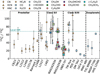 |
Fig. 1 Literature 12C/13C ratios towards sources at different evolutionary stages using different isotopologues. Simple O- and N-bearing species (<6 atoms) share a light blue and light yellow colour, respectively, but have different markers. Black rectangles around the orange triangle (N) and coloured circles (O) indicate complex organics (>6 atoms). Arrows indicate lower limits. References to the values can be found in Table A.9. |
List of sources from the PRODIGE sample towards which 13C isotopologues of CH3 OH and CH3 CN have been detected.
2 The PRODIGE data set
The PRODIGE large program is part of the MPG/IRAM Observatory Program (MIOP, Project ID L19MB) observed with NOEMA. A total of 30 Class 0/I protostellar systems were targeted, of which we study seven in this work (see Table 1 and Sect. 3). The observations were carried out using the Band 3 receiver and the PolyFix correlator, tuned to a local-oscillator (LO) frequency of 226.5 GHz. This setup provides a total bandwidth of 16 GHz with a channel width of 2 MHz, corresponding to ~2.5-2.8 km s−1. There are four sidebands: lower outer (214.7-218.8 GHz), lower inner (218.8-222.8 GHz), upper inner (230.2-234.2 GHz), and upper outer (234.2-238.3 GHz). In addition, 39 high spectral-resolution windows (62.5 kHz channel width), each covering a 64 MHz bandwidth, were placed within the 16 GHz bandwidth.
Observations were conducted in antenna configurations C and D and finished in 2024. In this work, we only used data taken in 2019 to 2022. The maximum recoverable scale (MRS) is 16.9″ at 220 GHz, which corresponds to approximately 5000 au at the distance of Perseus. The data calibration was done using the standard observatory pipeline GILDAS/CLIC3 package. We used 3C84 and 3C454.3 as bandpass calibrators and 0333+321 and 0322+222 as phase and amplitude calibrators. The observations for these calibrators were taken every 20 min. For the flux calibration we used LkHα 101 and MWC 349. The uncertainty in absolute flux density is 10%. Continuum subtraction and data imaging were done with the GILDAS/MAPPING package using the uv_baseline and clean tasks, respectively. The imaging of the spectral line cubes was done with natural weighting to minimise noise, while for the continuum maps we used robust = 1, to improve the angular resolution. More details on data reduction and imaging can be found in Gieser et al. (2024). The achieved angular resolution is ~1″, which corresponds to a spatial resolution of ~300 au. The accurate synthesised beams for each source as well as root-mean-square (rms) noise levels can be found in Table A.1.
3 Spectral line LTE analysis and results
We detected emission from the rarer 13C isotopologues of methanol and methyl cyanide towards seven and six protostellar sources of the PRODIGE sample (see Table 1), respectively. In this section we first present the morphology of the molecular emission and the position selection (Sect. 3.1), then discuss the line widths and peak velocities (Sect. 3.2). The following spectral line analysis is performed assuming a uniform medium that is in local thermodynamic equilibrium (LTE), which is applicable given the high volume densities (Yang et al. 2021). The spectral line identification and analysis were done using Weeds, which is an extension of the GILDAS/CLASS software (Maret et al. 2011). Weeds produces synthetic spectra by solving the radiative transfer equation. More details on the modelling with Weeds are in Sect. 3.3. The molecular column densities as well as the rotational temperatures that were obtained from this method are validated by results from a population-diagram analysis, which is described in Sect. 3.4. The results are presented in Sects. 3.5 and 3.6.
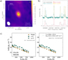 |
Fig. 2 Overview of the PRODIGE data towards IRAS 4B and presentation of the spectral line analyses. Panel a: integrated intensity map for th CH3CN 123−113 transition at 220.708 GHz. The beam (half power beam width, HPBW) is shown in the bottom left. The dashed yellow contou is at 5σ, where σ is the rms noise level and is written in the top-right corner. Panel b: observed spectra towards the peak position, which is a (Δα, Δβ = (0″, 0″) (black cross in panel a), of CH3CN at low (~2 MHz, black) and high (~62.5 kHz, teal) spectral resolution, where the latte] was shifted by 4K for visualisation. The low spectral-resolution data were analysed in this work (see Sect. 3). The modelled CH3CN spectra from Weeds are shown in red (low resolution) and orange (high resolution), where the same input parameters were used for both. Panel c: population diagram for CH3CN. Teal circles show the observed data points while the modelled data points from Weeds are shown with orange squares (se Sect. 4.6 for possible origins of differences between the two). No corrections are applied in the left panel, while in the right panel, corrections fo opacity and contamination by other molecules have been considered (negligible effect in this case), and only transitions with optical depths <0.5 (i.e. all transitions in this case) are shown. The results of the linear fit to the observed data points are shown in the right panels. |
3.1 COM emission morphology and position selection
As an example, Fig. 2a shows an integrated intensity map of CH3CN towards IRAS 4B. Integrated intensity maps of the 12C and 13C isotopologues of CH3OH and CH3 CN for all sources are shown in Figs. B.1–B.7. In most cases, the emission is compact and remains spatially unresolved in the PRODIGE data. Only for IRAS 4B, emission outside the compact hot-corino region is identified, which can be associated with its protostellar outflow (e.g. Sakai et al. 2012).
For the LTE analyses, we extracted the spectra at the continuum peak position at (0″ ,0″ ), which corresponds to the coordinates in Table 1. Although the line data may be affected by continuum optical depth, we did not select a position off peak (as done, for example, for IRAS 16293 by Jørgensen et al. 2016).
If we did so, we would risk to detect fewer transitions, which might, in turn, result in larger uncertainties in the LTE analyses as both methods require as many lines as possible.
3.2 Line widths and peak velocities
For the spectral line analyses (Sects. 3.3 and 3.4), we made use of the low spectral-resolution (LR) data that covers the total 16 GHz bandwidth and hence more spectral lines of our molecules of interest. However, because of the narrow line widths of the spectral lines (full width at half maximum, FWHM, of <4 km s−1, see Tables A.2–A.8) they are only marginally spectrally resolved if at all. To determine the true FWHM and peak velocity, we used the higher resolution (HR) data. The HR data only cover transitions of both methanol isotopologues in their vibrational ground state, while the LR data also cover vibrationally excited states. Figure 3 shows peak velocities, νpeak, and FWHM, which we derived from 1D Gaussian fits to all available transitions, as a function of upper-level energy, Eu. The median values for both species are shown with dashed lines. Outliers may appear as a consequence of weak transitions or unidentified contamination by other species, which can lead to shifts. In addition, Fig. 3 only shows transitions with τ < 10, though some FWHM may be larger due to optical depth effects. For some sources, the presence of outflow wing emission may broaden the lines. In some cases, there are significant differences between 12C and 13C methanol, which may indicate that the two species probe different material along the line of sight. Higher spectral resolution data that cover a larger number of spectral lines per species will help draw conclusions on this.
In the following, we ignore possible kinematic differences between species and use an effective FWHM, that is the lower median between the two species, and the respective νpeak value. Because of their unresolved hyperfine structure, methyl cyanide isotopologues are not used to determine line properties. However, the hyperfine structure (HFS) is considered later during the determination of column densities, except for 13CH3CN, as the Cologne database of molecular spectroscopy (CDMS; Endres et al. 2016), from which all spectroscopic data were taken, does not include the HFS for frequencies beyond 220 GHz.
 |
Fig. 3 Peak velocity, νpeak, and line width, FWHM, derived from 1D Gaussian fits (including 1σ error bars) to the high spectral-resolution (HR) PRODIGE data as a function of upper-level energy, Eu, for the vibrational ground states of CH3 OH (orange) and 13CH3OH (teal). The coloured dashed lines indicate the respective average values for νpeak and FWHM. |
3.3 Radiative transfer modelling with Weeds
We classify a molecule as detected when there are at least five transitions per isotopologue in the observed LR spectra above an intensity threshold of 3σ, where σ is the rms noise level measured in the 3D data cubes (see Table A.1), and the modelled spectra reasonably reproduce these transitions. In order to derive a synthetic spectrum for a molecule, Weeds requires five input parameters: total column density, rotational temperature, source size, FWHM, and velocity offset, νoff = νpeak,HR - νsys, of the spectral line from the source systemic velocity, where νsys is taken from Table 1. The FWHM and νpeak,HR present observed values, for which we ignore any unresolved kinematic substructures and velocity gradients, and were determined from 1D Gaussian fits in Sect. 3.2. For FWHM that are spectrally unresolved in the observed LR spectra, Weeds smooths the line width for the given channel width. The source size, that is the size (in arcseconds) of the emitting area is needed to compute the beam filling factor.
We adopted source sizes from the literature (Table 1), which were estimated from COM emission (Belloche et al. 2020; Chen et al. 2024) or, if this was not available, from continuum emission (Yang et al. 2021). Because Weeds does not perform a fit to the observed data, the total column density, Ncol, and the rotational temperature, Trot, were adjusted in an iterative way: starting from a first educated guess, population diagrams (see Sect. 3.4) were derived and the resulting values for Ncol and Trot were fed back into Weeds. This was repeated until both Weeds and the population diagrams provide matching results for Ncol and Trot within the uncertainties. In the process, Weeds computes line optical depths and takes it into account when creating the model spectrum, based on the input parameters. We used this opacity correction when deriving population diagrams (see Sect. 3.4). The parameters of all final models are summarised in Tables A.2–A.8. In Fig. 2b we show, as an example, a spectrum of CH3CN towards IRAS 4B from the low (black) and high (teal) spectral resolution PRODIGE data. The former is used for the spectral line analysis because a wider bandwidth and hence a larger number of transitions was covered. The derived Weeds model is shown in red. For comparison, we also show the model of the high resolution case in orange.
It happens that the final model over- or underestimates the peak intensity for a few transitions, even if it (and the corresponding population diagram) matches well the rest of the observed spectrum. If the model underestimates the intensity, this likely indicates contamination by another species that adds to the observed intensity. In severe cases, the line is excluded from further analysis. It may also be that the intensity of a transition is not well estimated by the model because the observed emission is not described by a single excitation temperature. This cannot be accounted for in the Weeds models (nor the population-diagram analysis) and can result in an over-or underestimation by the model. Especially, transitions with lower upper-level energies suffer from this effect as they can be excited more easily. Deviations from Gaussian profiles caused by such a non-uniform medium or optical depth effects may be worsened due to spectral dilution in the LR data. Such limitations of this analysis and their consequences are taken up on in Sect. 4.6.
3.4 Population diagrams
To verify total molecular column densities, Ntot, and rotational temperatures, Trot, used to derive the synthetic spectra, we derived population diagrams (PDs), which are based on the following formalism (Goldsmith & Langer 1999; Mangum & Shirley 2015):
 (5)
(5)
where Nu is the upper-level column density, gu the upper-level degeneracy, Eu the upper-level energy, Au the Einstein A coefficient, kB the Boltzmann constant, c the speed of light, h the Planck constant,  the beam filling factor, and Q the partition function. Intensities in brightness temperature scale, J(TB), are integrated over a visually selected velocity range, dν, in the continuum-subtracted spectra. When computing the left-hand term for each transition of a species and plotting it against Eu, all data points should ideally follow a linear trend, in which case the level populations can be explained by a single rotational temperature.
In Fig. 2c we show one PD of CH3CN obtained for IRAS 4B as an example (all other PDs can be found in Figs. C.1–C.8 in the appendix). Both the observed data points as well as those derived from the Weeds models are shown. If detected, rotational transitions from vibrationally excited states (v = 1, v = 2 for CH3OH and v8 = 1 for CH3CN) are used in addition to transitions from the vibrational ground state (v = 0). The left panel shows the original data obtained from Eq. (5), while two correction factors (i.e. optical depth and contaminating emission, see below) are applied to the modelled and observed data in the right panel (negligible effect in Fig. 2c). One of the correction factors considers line opacities. Besides computing the synthetic spectra for a molecule, Weeds also calculates the optical depth for each transition for the given input parameters. Using the respective peak opacity from Weeds, τi, for a given transition i, we computed a correction factor,  (e.g. Mangum & Shirley 2015). This factor was then multiplied by the observed and modelled integrated intensities. However, the right-hand panels of the PDs only show transitions for which Weeds computes optical depths of <0.5. Plus, the linear fit is only applied to those data points. Since it is possible that we still underestimated optical depth for some lines (see Sect. 4.6), we did not use transitions with higher opacities to ensure that the fit parameters apply to the sufficiently optically thin lines.
Secondly, contaminating emission from other species was subtracted from the integrated intensities, if identified. In particular, this applies to CH3CN and CH313CN, which have overlapping transitions at ~220.636 GHz. Assuming that the emission spatially coincides, this addition of spectra from different species and a subsequent subtraction of contaminating emission only works for optically thin transitions. Even with the two correction factors applied, some scatter between the observed and modelled data points remains. In the example in Fig. 2c, the model clearly underestimates the observations. This is a result of the narrow line widths. As can be seen from the spectra in Fig. 2b, the spectral lines are rarely broader than one channel. However, for the integration we used at least 2-3 channels, adding contaminating emission that seems to be an additional CH3CN component in the case of IRAS 4B, possibly associated with its outflow. Observational limitations such as these are discussed in detail in Sect. 4.6.
The linear fit is applied to the corrected observed data without taking into account their displayed uncertainties, since not all of them can be quantified, such as possible contamination from unidentified species. The displayed error bars only include the standard deviation from integrating intensities and the 10% uncertainty in absolute flux density. From the linear fit, we obtain Trot from the slope and Ntot from the y-intercept. The latter requires knowledge of Q(Trot), which is taken from the CDMS4, together with other spectroscopic information, such as Au, Eu, and the rest frequencies.
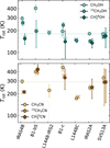 |
Fig. 4 Rotational temperatures used for the Weeds modelling (crosses) and derived from the population diagrams (circles with 1σ error bars). The dashed lines indicate the median values considering all isotopologues of a species. |
3.5 Rotational temperatures and 12C/13C isotopologue ratios
Figure 4 compares the rotational temperatures derived from both the Weeds modelling and the PDs for the various isotopologues in each source. In all shown cases, the temperatures derived from both methods agree within the error bars. Large error bars result from a smaller number of mostly weak transitions that were available to derive the respective PD. Some PD temperatures are not shown either because the molecule was not detected (both 13C CH3CN isotopologues towards L1448-IRS2) or because the PD fit was unreliable and Trot was fixed in the PDs to a value from the other detected species (see Tables A.2–A.8).
Overall, the results show that, for most sources, CH3CN has higher temperatures than CH3OH. The median rotational temperature derived from methanol is 180K (140-400 K), that from methyl cyanide is 290K (180-420 K). In some cases, the temperature values for the respective isotopologues are different. For example, for B1-bS and IRAS 2A, CH3 OH shows higher temperature than 13CH3OH. This similarly applies to the CH3CN isotopologues for IRAS 4B. This may indicate that the isotopologues probe different excitation conditions.
Table 2 summarises the 12C/13C isotopologue ratios computed from the Weeds column densities of CH3OH and CH3CN for the PRODIGE sample sources. The ratios are shown in comparison to other sources in Fig. 5, where we used an average value for the two 13C isotopologues of methyl cyanide. The error bars are those from the linear PD fits. The ratios range from 4 to 30 and are thus all significantly below the local ISM value of 68. There is no significant difference between CH3 OH and CH3 CN. In some cases, uncertainties are likely larger than depicted (see Sect. 4.6).
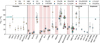 |
Fig. 5 Same as Fig. 1 but including the 12C/13C ratios derived from the PRODIGE data in this work (light red shaded). Bolometric luminosities of the protostars increase from left to right. Black rectangles around markers indicate complex organic molecules. Arrows indicate lower limits. |
Column density ratios for CH3 OH and CH3 CN isotopologues derived from the Weeds models.
3.6 CH318OH
The 18O methanol isotopologue is detected towards four of the seven sources of our sample: SVS13A, IRAS 2A, IRAS 4B, and B1-c. We applied the same analysis to this molecule: synthetic spectra were derived by fixing all parameters to those of 13CH3OH, except for the rotational temperature and column density. Population diagrams can be found in Fig. C.8.
The derived rotational temperatures (Fig. 4) remain below 200 K and are hence either comparable to or lower by a few tens of Kelvin than the other CH3OH isotopologues. Figure 6 shows the resulting column density ratios between 13CH3OH and CH318OH together with lower limits on this ratio for the sources towards which the latter species remains undetected. Based on the local ISM value of 16O/18O = 557 (e.g. Nomura et al. 2023), we expect  , which is consistent with our results within the error bars.
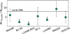 |
Fig. 6 Column density ratio between 13CH3OH and CH318OH using the Weeds column densities. The expected local ISM value of ~8 is indicated with a dashed line. Arrows show lower limits. |
4 Discussion
4.1 Low 12C/13C COM isotopologue ratios in other protostellar systems
Low 12C/13C ratios for (COM) isotopologues towards protostellar systems have been reported in the past. Using the PRODIGE data, Hsieh et al. (2023) derived a similarly low 12C/13C ratio (~15—25) for CH3CN towards the binary protostellar system SVS13A. These authors tested whether modelling one or two excitation components would lead to a different outcome, which it did not, as low ratios were seen in either scenario. In a followup study at much higher angular resolution with the Atacama Large Millimetre/submillimetre Array (ALMA) the molecular emission was resolved and the low 12C/13C ratios for CH3CN were confirmed (Hsieh et al. 2025) towards one of the protostars.
Based on data obtained with ALMA at ~0.5″ angular resolution as part of the Protostellar Interferometric Line Survey (PILS) towards the young protostellar triple system IRAS 16293-2422 (IRAS 16293 hereafter), Jørgensen et al. (2016) reported 12C/13C ratios of 24-35 for the glycolaldehyde (CH2OHCHO) isotopologues towards IRAS 16293B. Based on the same observational data, low 12C/13C isotopologue ratios were also (tentatively) found for C2H5OH, CH3OCHO, and CH3OCH3 (see Fig. 5 and Jørgensen et al. 2018). These three O-bearing molecules, together with glycolaldehyde and methanol, likely form in the solid phase during the cold prestellar stage as predicted by astrochemical models (e.g. Garrod et al. 2022). They are formed from CO that was previously enriched with 13C via the exchange reaction (Eq. (1)) in the cold gas phase prior to freeze-out. This similarly applies to CH3CHO, which can be formed in the solid phase from CH2CO, which in turn is formed from CO (e.g. Ibrahim et al. 2022; Garrod et al. 2022). However, these two species and t-HCOOH, whose formation also includes CO, have 12C/13C ratios close to the local ISM value in IRAS 16293B, based on the PILS data. At temperatures >100 K, CH3CHO has an efficient formation route in the gas phase (C2H5 + O, e.g. Garrod et al. 2022), which might explain why its 12C/13C ratio is different from the other O-bearing COMs, that is, if the ratio for C2H5 were as high. Again using the PILS data, Calcutt et al. (2018) derived 12C/13C for the CH3CN isotopologues of ~70-80 in IRAS 16293A and B, which is in contrast to our results. Differences between starforming regions in the 12C/13C ratio of a given species may be linked to the duration of the prestellar phase as indicated by models (see Sect. 4.5).
The 12C/13C COM isotopologue ratio has also been investigated within the framework of the ALMA Survey of Orion Planck Galactic Cold Clumps (ALMASOP; Hsu et al. 2020, 2022) at an angular resolution of −0.4″. Of the 72 targeted clumps (some containing multiple pre- and protostellar sources) 56 Class 0/I protostars have been identified (Dutta et al. 2020), of which eleven show warm methanol emission (Hsu et al. 2022). For another six of these sources, 13CH3OH has been detected. The resulting 12C/13C ratios are all below 5, likely because not many methanol transitions are covered in the survey resulting in a strong underestimation of the main isotopologue’s optical depth.
Recently, low 12C/13C ratios of 20-30 have also been measured for several O-bearing COMs towards the V883 Ori disk (Yamato et al. 2024; Jeong et al. 2025), based on ALMA data at 3 mm. Similar to the considerations done for IRAS 16293, the authors argue that one possible reason may be the COMs’ formation from CO in ices at early stages, where CO was enriched in 13C prior to freeze-out, but further investigation is needed.
4.2 No evidence for an O/N dichotomy based on the 12C/13C ratio
We selected CH3OH and CH3CN for this work because they trace the warm gas towards the protostellar sources and to study a possible segregation between the O- and N-bearing molecules based on their 12C/13C isotopologue ratios. For the disk around the T Tauri star TW Hya (see Sect. 1 and, e.g., Bergin et al. 2024), low 12C/13C ratios were derived for CO inside a 100 au radius and ratios close to or higher than the local ISM value for C2H, HCN and CN (see also Fig. 5). The presence of two different carbon isotopic reservoirs was proposed as the origin for this dichotomy. Disk simulations (Lee et al. 2024) were able to reproduce the various 12C/13C isotopologue ratios when considering C/O > 1. In this work, we explored whether there is any difference between CH3OH and CH3CN in terms of the 12C/13C ratio at the Class 0 stage. First evidence for this can be seen from the ratios derived towards IRAS 16293B (see Sect. 4.1 and Fig. 5), where (some) O-bearing COMs show an enhancement in 13C, while CH3CN shows ISM-like values. Our results do not show significant differences between CH3OH and CH3CN (Fig. 5). It is worth mentioning that for some sources the rotational temperatures that we derived for the CH3OH and CH3CN isotopologues were different. This may indicate that they probe different excitation conditions. This effect on the 12C/13C ratio and others that arise from observational limitations (see Sect. 4.6) can be tackled in observations at higher angular and spectral resolution.
4.3 Implications of the 13CH3OH/CH318OH ratio
The local ISM 16O/18O isotopic ratio is 557 ± 30 (Wilson 1999). Dividing this value by the 12C/13C ratio of 68, yields a theoretical 13C16O/12C18O ratio of –8, which agrees with the values that we derived for CH3OH towards the PRODIGE sources within the error bars (see Fig. 6). Therefore, based on this isotopologue ratio, we do not expect an enrichment in 13C, which may imply that we are underestimating the column density of the main isotopologue. As mentioned in Sect. 4.2, differences in rotational temperatures between CH3OH isotopologues may affect the ratios.
Regarding the robustness of the 13C16O/12C18O ratios, lower values would mean that the abundance of CH318OH is enhanced, which has not been reported so far. On the contrary, oxygen fractionation is proposed to be a consequence of isotope-selective photodissociation that depletes CO-related molecules in 18O (e.g. Nomura et al. 2023). Loison et al. (2019) modelled the 16O/18O ratio in dark cloud conditions and compared it with observations. They found that in order for molecules to be enriched in 18O, the isotope has to be abundant in the gas phase. Consequently, only a small fraction would be available in ices. They focussed on S-bearing species, but also computed the 16O/18O for CO and CH3OH in the gas phase as a function of time and find no significant deviations from the local ISM value. More simulations are needed to ascertain whether this remains to be the case during the protostellar phase.
The 13C16O/12C18O ratios have recently been determined for Class II sources, which were observed as part of the PRODIGE - Planet-forming disks in Taurus with NOEMA (Semenov et al. 2024). They were mostly found to be close to the expected value of 8, in agreement with the ratios that we found at earlier stages, although some of the Class II disk systems are rather described by isotopologue ratios deviant from the ISM values, according to simulations (Franceschi et al. 2024).
4.4 Tentative evidence for an O/N temperature segregation
Segregation between O- and N-bearing molecules is frequently observed (e.g. Widicus Weaver et al. 2017; Allen et al. 2017; Jørgensen et al. 2018; Csengeri et al. 2019; Pagani et al. 2019; Busch et al. 2022, 2024; Bouscasse et al. 2024), either in terms of spatial variations in their emission or in terms of differing rotational temperature and abundance. We derived on average higher rotational temperatures (Fig. 4) for the CH3CN (290 K) than for the CH3OH isotopologues (180 K), implying that the two species probe different conditions in the gas, which may trace back to their dominant formation and destruction mechanisms.
Methanol gas-phase abundances are predicted to peak at ~ 100150K (Garrod et al. 2022). At these temperatures the COM thermally desorbs from the icy dust grains, where it was formed prior to the birth of the protostar via successive hydrogenation of CO. Due to a lack of efficient gas-phase formation routes, the COM was found to be destroyed in the high-temperature gas phase right after its desorption (Garrod et al. 2022; Busch et al. 2022). On the other hand, methyl cyanide can efficiently be produced at high temperatures in the gas phase (Garrod et al. 2022). Another process that may explain this difference is carbon-grain sublimation (van’t Hoff et al. 2020, see also Nazari et al. 2023 and van’t Hoff et al. 2024). It was proposed to result in enhanced abundances of N-bearing COMs at temperatures >300 K through release of more refractory C- and N-rich species from the grain mantle.
Some of our analysed sources were also covered in the analysis of the spectral line data obtained as part of the IRAM Plateau de Bure Interferometre (PdBI) large program CALYPSO (Continuum And Lines in Young ProtoStellar Objects; Belloche et al. 2020). This survey resembles the PRODIGE survey in angular and spectral resolution but covers a smaller bandwidth. The authors used the same methods of analysis as in this work and do not find a significant difference in rotational temperature between O- and N-bearing molecules in general. Their values are likely more uncertain because they cover fewer transitions and a smaller range of upper-level energies. The authors do not report column densities for the rarer isotopologues of CH3 OH and CH3CN. Their column densities of the main isotopologues agree within a factor of 2 with ours, except for SVS13A and IRAS 2A, for which we derived methanol column densities that are a factor of 5.5 and 8 higher, respectively, than reported by Belloche et al. (2020). We assumed a source size of 0.2″ (Chen et al. 2024) for IRAS 2A, whereas Belloche et al. (2020) used 0.35″, resulting in a threefold difference in the column densities. The remaining difference is likely attributed to optical depth. According to our Weeds models for the two sources, all methanol transitions with Eu < 600 K show opacities above 0.5. Hence, we did not include them in the PD fits. In contrast, Belloche et al. (2020) use all transitions, likely resulting in an underestimation of the column density.
4.5 Comparison with astrochemical models
We ran simulations of carbon and nitrogen isotopic fractionation using the gas-grain chemical code pyRate, whose basic properties are described in Sipilä et al. (2015). We employed the gas-phase and grain-surface chemical networks presented recently in Sipilä et al. (2023), where an extensive set of isotopic exchange reactions for C- and N-bearing species - also taking into account the possibility of simultaneous isotopic substitution in both elements (e.g. H13C15N) - is considered, though in the present paper we do not provide predictions for 15N-bearing species. The networks, however, only include species consisting of up to five atoms; hence, we cannot obtain direct estimates for the fractionation of CH3OH and CH3CN. Instead, we simulated the abundances of precursor species and used them to estimate the isotopic ratios of CH3 OH and CH3CN, based on their most likely formation pathways, to constrain the possible origins of the low ratios derived for these COMs from the present observations.
We have not attempted to simulate each observed source individually. Instead, we have adopted as a template the physical model for the protostellar core IRAS 16293-2422 presented by Crimier et al. (2010), and carried out chemical simulations to predict the 12C/13C ratios of various species. Here, we give a brief account of the model setup; an expanded description including the initial conditions is given in Appendix D. Following Brünken et al. (2014) and Harju et al. (2017), we have employed a two-stage approach where the chemistry first evolves over a period of 106 yr in an intermediate-density dark cloud, and then for another period of 104 yr in the protostellar conditions using the abundances obtained in the first stage as initial abundances for the second stage. For simplicity, the primary cosmic-ray ionisation rate was set to the canonical value of ζp = 1.3 × 10⁻¹⁷ s−1 across the core5. The initial elemental 12C/13C ratio is set to 68 in the first stage (Milam et al. 2005). The model of Crimier et al. (2010) is not appropriate for describing the very innermost regions of the protostellar core (inside a few hundred au) but is applicable in the present context where the observations have not been carried out using high angular resolution.
Figure 7 shows the 12C/13C ratios for various CH3OH and CH3CN precursors as a function of distance from the centre of the protostellar core, taken at the simulation time t4 = 104 yr in the second (i.e. protostellar) stage of the simulation. We only show this time step because the ratios do not change significantly at later stages, except for H2CO (see below). The complex features evident in the various ratios as a function of radius, especially prominent at radii in the range 1000-2000 au, are a result of complex interactions involving different binding energies between the species, isotopic exchange reactions etc. Quantifying these is outside the scope of the present paper, where we concentrate only on the innermost regions of the core (left of the vertical dotted line in Fig. 7) and analyse the general trends. In what follows, we discuss the results for species associated with methanol and methyl cyanide separately.
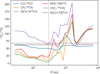 |
Fig. 7 Model predictions for selected gas-phase 12C/13C ratios as a function of distance from the protostar taken at a simulation time of 104 yr. The constant ratio of 68 is indicated by the horizontal dashed black line. The vertical dotted black line separates the spatial scales discussed in this paper (R < 300 au) from the larger scales, which are not largely discussed but shown for completeness. |
4.5.1 Methanol (precursors)
Methanol is formed during the prestellar phase in the ice mantles of dust grains through successive hydrogenation of CO.
Figure D.1 shows the evolution of the 12C/13C ratio during the prestellar phase, indicating that, as time advances, the 12CO/13 CO ratio approaches the ISM value of 68 in both gas and ice. We would expect the ratio for methanol to follow a similar trend, so that, when CH3OH sublimates from the ices, the value should not be too different from what is seen at the end of the prestellar stage. This is higher than what we observe. It may be that the observed protostellar systems spent a shorter time in the prestellar phase than assumed in the model, thereby inheriting lower 12C/13C ratios (Fig. D.1). Such a time dependence may also explain the differences in the 12C/13C ratios seen between the Perseus sources and, for example, IRAS 16293 (see Sect. 4.1). However, the 12CO/13CO ratios are significantly lower only for t < 105 yr. Predictions by Ichimura et al. (2024) show that, between 105−106 yr, the 12C/13C ratio for CH3OH in ices during the prestellar phase can be somewhere between 40-60. Hence, although a shorter prestellar phase may not solely explain our observed ratios of <30, it can still affect the observed 12C/13C ratios observed during the protostellar stage. In Section 4.6 we discuss that the column densities of especially the main isotopologue of methanol derived from observations can be underestimated due to an underestimation of optical depth, and hence the 12C/13C ratios may be higher. A final conclusion needs further observational and computational efforts.
Moreover, the 12C/13C ratios close to the local ISM value for CO as predicted by the current simulations are in agreement with observations of ices in the ISM (Brunken et al. 2024, see their Fig. 10, and references therein). In addition, we note that our simulation predictions for the 12CO/13CO ratios are similar to those presented recently by Bergin et al. (2024) and Ichimura et al. (2024); the latter authors predicted a CH3OH 12C/13Cratio close to that of CO (below 68).
One intermediate product of the methanol formation in ices is formaldehyde (H2CO), which is included in the model. Its gasphase 12C/13C ratio is shown in Fig. 7 and is ~62 at the scales traced by our observations (i.e. a few 100 au). The slight difference between the CO and formaldehyde 12C/13C ratios likely results from competition between the formation of H2CO in the solid phase from CO and in the gas phase; an in-depth examination of the simulation results shows that the H2CO 12C/13Cratio rises in the central core at later times (not shown) due to a chain of chemical reactions starting with desorbed CH4.
4.5.2 Methyl cyanide (precursors)
The pathway(s) that dominate the formation of CH3CN are much less certain. Recently, the gas-phase chemical network of the COM has been revised by Giani et al. (2023). They used quantum-mechanical calculations to test the relative importance of the various proposed formation routes of CH3CN. Their results suggest that the COM is dominantly formed from protonated methyl cyanide (CH3CNH+) that recombines with an electron or gives the extra proton to NH3 upon reaction. Protonated CH3CN is in turn a product of the reactions CH3+ + HCN and CH3OH2+ + HNC. Methyl cyanide can also form on dust grain surfaces via CH3 + CN and hydrogenation of CH2CN (e.g. Garrod et al. 2022).
In Fig. 7, we show 12C/13Cratios for CN, HCN, HNC, and CH3+. The first three follow a similar trend: the ratio is significantly below the local ISM value at close distances to the protostar and only increases to above the ISM value beyond 500-1000 au. This is a result of exchange reactions such as Eqs. (2)–(4), whose relative importance depends on time and the prevalent physical conditions. On the other hand, the simulated 12C/13C ratio of CH3+ is approximately 100 in the inner core, and therefore, if the CH3+ + HCN formation pathway is dominant, we may expect 13CH3CN and CH313CN to show different fractionation levels. Only for IRAS 4B, is there tentative evidence for a different ratio (factor of 2, see Table 2); however, due to the small number of transitions (<5) available for the rare CH3CN isotopologues, we cannot be certain.
Therefore, the CH3OH2+ + HNC formation pathway thus seems more likely, but we cannot quantify this expectation with the present model. Similarly, the model predicts a high (~ 100) 12C/13C ratio for CH3 ice and a low ratio (~30) for CN ice at the end of the cloud stage (Fig. D.1), indicating a similar dichotomy between 13CH3CN and CH313CN if they were predominantly formed on grains via the association of CH3 and CN. An expanded chemical model, taking into account isotopic fractionation of COMs, is required to draw definite conclusions on the 12C/13C ratios, also keeping in mind that the physical model used in the present work is extremely simple.
Our simulation predictions for the 12C/13C ratios for CN, HCN, and HNC are contrary to those presented recently by Ichimura et al. (2024). In their Fig. B5, the authors show that the ratios for these species and CH3CN remain elevated (80-90) throughout the protostellar phase. During the prestellar phase, the 12CN/13CN ratio behaves similarly in our and their models. It is not clear whether this discrepancy in the protostellar phase is due to the warm-up scenario considered in their model versus our static approach or to differences in the chemical network. A detailed investigation is outside the scope of the present paper.
4.6 Observational limitations
In Sect. 3.4 we already mentioned that scatter between the observed and synthesised data points in the population diagrams (PDs) shown in Figs. C.1–C.8 arises from the integration of intensities over at least three channels. Hence, by using the LR data (with a channel width of ~2MHz) for the analysis, integrated intensities for lines that are spectrally unresolved (i.e. FWHM ≲ channel width) will inevitably contain some contamination or extra noise. Contamination may come from unidentified species or unresolved additional velocity components from the same species (e.g. outflow emission; see Fig. 2b). In addition, the optical depth of optically thick lines may be underestimated by the model due to the spectral dilution as the true line profiles remain unknown. This fact together with line optical depths that generally exceed the capability of the Weeds model to correct for them (τ & 2) are the main reasons for the discrepancy between transitions with low and high upper-level energies for sources with highest molecular column densities (e.g. for CH3OH Eu ≲ 600 K for B1-c, IRAS 2A, and SVS13A).
An overall underestimation of a molecule’s column density may be a consequence of high continuum optical depth. If the continuum was optically thick, it would partially obscure the line emission (De Simone et al. 2020). Recent ALMA observations towards IRAS 2A and B1-c (Chen et al. 2024) at 0.9 mm showed that the continuum is indeed optically thick towards the central position of IRAS 2A, however, the effect is negligible for B1-c. The PRODIGE data cover lower frequencies, therefore, continuum opacities are generally lower. We cannot exclude a contribution of this effect to the uncertainties for some (i.e. the brightest) sources, but it does not apply to all. Observations at lower frequencies will help constrain the continuum optical depth at our observed frequencies.
Another source of uncertainty comes from the spatially unresolved emission. An overestimation of the size of the emitting area will lead to an underestimation of the column density. If the emission is optically thick or includes unresolved structures for one but not the other isotopologue, this can also affect the column density ratios. Moreover, we do not resolve any morphological structures, such as binaries (e.g. SVS13A, Hsieh et al. 2025, and IRAS2A, Jørgensen et al. 2022), streamers (e.g. Valdivia-Mena et al. 2024), or outflows (e.g. Podio et al. 2021, see also the HR spectrum in Fig. 2b, which shows outflow wing emission for IRAS 4B). These may come with different velocity components that we are not able to spectrally resolve, either, but rather smooth over. Accordingly, spatial variations in the 12C/13C ratios can likely be expected. Therefore, we may only see an average ratio in the current observations, which may not reflect the true conditions at all.
Lastly, although we are correcting for line opacities and focus the analysis on the optically thin(ner) lines, there is still a chance that we are underestimating the values, as they are model-dependent. Ultimately, observations at higher angular and spectral resolution that simultaneously cover a broad bandwidth are needed to address these issues and to put better constraints on the 12C/13C ratios.
5 Conclusions
We aimed to increase the number of measurements of 12C/13C ratios in the warm gas around young embedded protostellar systems using the data obtained as part of the PRODIGE large program. The 13C isotopologues of CH3OH and CH3CN were detected towards seven and six sources, respectively, out of a total of 30 Class 0/I protostellar systems targeted by the PRODIGE survey. By using isotopologues of these complex organic molecules (COMs), we ensured that the molecular emission stems from the innermost hot gas surrounding the proto-star(s). Additionally, we could test whether there is a segregation between O- and N-bearing molecules in terms of the 12C/13C ratio. Our main findings are the following:
We derived excitation conditions and column densities using optically thin(ner) spectral lines assuming LTE;
The resulting 12C/13C column density ratios for CH3 OH and CH3CN range from 4 to 30, which is lower than the expected ISM value of 68 by factors of a few up to an order of magnitude;
There is tentative evidence for an O/N segregation based on rotational temperatures, where CH3CN isotopologues trace warmer gas on average (290 K) than CH3OH (180 K). This may hint at the dominant formation pathways of the two COMs on dust grain surfaces during the prestellar phase (CH3OH) or in the hot gas phase (CH3CN);
There is no significant difference between the 12C/13C ratios from CH3 OH and CH3 CN. This is in contrast to the ratios derived in previous works from COMs towards the Class 0 protostellar system IRAS 16293-2422. In this source, some O-bearing COMs show 12C/13C ratios as low as ours, however, the values from CH3CN isotopologues are around the ISM value. The origin of differences between the various molecules among different star-forming regions is not yet understood and requires further observational and modelling efforts;
Astrochemical models that we conducted for potential precursor molecules of CH3OH and CH3CN predict 12C/13C ratios for CO and H2CO that are close to or slightly below the local ISM value of 68 (in ice and gas). The ratios do not reach as low as in the observations. One reason may be the assumed duration of the prestellar phase in the model (106 yr), but this requires further investigation. The gasphase 12C/13C ratios for CH3CN precursors, in particular CN, HCN, and HNC, are predicted to be in the range 20-50 at the spatial scales probed by the observations (~300 au), more similar to the observational results for CH3CN.
Our observational and modelling results indicate that there exists 13C enrichment at the Class 0 stage traced by COMs, which likely originates from the prestellar stage. There are some observational limitations, which we evaluated in detail, that come with the spatially and (mostly) spectrally unresolved PRODIGE data set and that can be addressed in future wideband observations at higher angular and spectral resolution. Nevertheless, our work opens the avenue to using the 12C/13C ratio to study the question of chemical inheritance, as protostellar and protoplanetary disks are likely to inherit at least some fraction of the parent cloud material.
In addition, our simulations predict that the 12C/13C ratios for simpler species, such as H2CO, HCN, or HNC, greatly vary as a function of distance from the protostar (i.e. density and/or temperature) and depend on the duration of the preceding prestellar phase. An in-depth study of these isotopologues will shed light onto the dependence of the 12C/13C ratios on time and environment and may help put constraints on the chemical network of more complex species such as CH3CN.
Acknowledgements
The authors thank the IRAM staff at the NOEMA observatory for their support in the observations and data calibration. This work is based on observations carried out under project number L19MB with the IRAM NOEMA Interferometer. IRAM is supported by INSU/CNRS (France), MPG (Germany) and IGN (Spain). L.A.B., J.E.P., O.S., P.C., M.J.M., C.G., M.T.V.M., Th.H., D.S., and Y.C. acknowledge the support by the Max Planck Society. A.F. and J.J.M.P. acknowledge support from ERC grant SUL4LIFE, GA No. 101096293. Funded by the European Union. Views and opinions expressed are however those of the author(s) only and do not necessarily reflect those of the European Union or the European Research Council Executive Agency. Neither the European Union nor the granting authority can be held responsible for them. A.F. also thanks project PID2022-137980NB-I00 funded by the Spanish Ministry of Science and Innovation/State Agency of Research MCIN/AEI/10.13039/501100011033 and by “ERDF A way of making Europe”. Th. H. and D. S. acknowledge support from the European Research Council under the Horizon 2020 Framework Program via the ERC Advanced Grant Origins 83 24 28 (PI: Th. Henning). L.C. acknowledges support from the grant No. PID2022-136814NB-I00 by the Spanish Ministry of Science, Innovation and Universities/State Agency of Research MICIU/AEI/10.13039/501100011033 and by ERDF, UE.
Appendix A Additional tables
Table A.1 lists beam sizes and rms noise values for the seven sources of the PRODIGE sample studied in this work. Tables A.2–A.8 contain the parameters to derive the LTE radiative transfer models for each analysed molecule as well as the results from the population-diagram analysis. The literature 12C/13C ratios for all additional sources shown in Figs. 1 and 5 are listed in Table A.9 together with their respective reference and the species that were used to derive them.
Information on the PRODIGE observations.
Weeds parameters and results of the population-diagram analysis for IRAS 2A.
Appendix B Additional figures: Integrated intensity maps
Figures B.1–B.7 show integrated intensity maps for selected transitions of the main and rarer isotopologues towards the seven sources of the PRODIGE sample that were analysed in this work. The transitions were selected because they are bright and unblended.
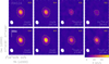 |
Fig. B.1 Integrated intensity maps using two transitions for both isotopologues of CH3 OH, the main CH3CN isotopologue, and one transition for each of the 13C isotopologue towards IRAS 2A. Respective rest frequencies (in GHz) are shown in the bottom-right corner, the beam (half power beam width, HPBW) on the bottom left. Multiplication factors (e.g. ×3, next to the species name) were applied to some species and transitions to be able to use the same intensity scale for all panels. The yellow dashed contour is at 5σ, where σ is the rms noise level (in K km s−1) and is written in the top-right corner. |
Appendix C Additional figures: Population diagrams
In Figs. C.1–C.8 all derived population diagrams are displayed.
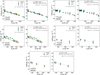 |
Fig. C.1 Population diagrams for CH3 OH, 13CH3OH, CH3CN, 13CH3CN, and CH313CN towards IRAS 4B. Observed data points are shown with teal circles as indicated in the top-right corner of the left panel while the modelled data points from Weeds are shown as orange squares. No corrections are applied in the left panels while in the right panels corrections for opacity and contamination by other molecules have been considered for the observed and modelled populations. The results of the linear fit to the observed data points are shown in the right panels. |
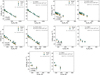 |
Fig. C.2 Same as C.1 but for L1448C. |
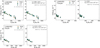 |
Fig. C.3 Same as C.1 but for L1448-IRS2. |
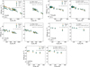 |
Fig. C.4 Same as C.1 but for B1-c. |
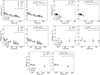 |
Fig. C.5 Same as C.1 but for B1-bS. |
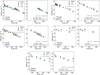 |
Fig. C.6 Same as C.1 but for IRAS 2A. |
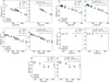 |
Fig. C.7 Same as C.1 but for SVS13A. |
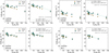 |
Fig. C.8 Same as C.1 but for CH318OH towards IRAS 2A, IRAS 4B, SVS13A, and B1-c. |
Appendix D Details of the chemical and physical models
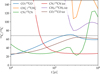 |
Fig. D.1 Model predictions for selected gas-phase and ice 12C/13C ratios as a function of time in the first simulation stage, representing evolution in dark cloud conditions. |
As noted in Sect. 4.5, we have performed the chemical simulations in two stages. In the first (dark cloud) stage, we have run a simple point (i.e. zero-dimensional) model to represent chemical evolution in a dark cloud, assuming canonical physical conditions n(H2) = 104 cm−3, Tgas = Tdust = 10K, AV = 10 mag. The chemistry was let to evolve over a period of 106 yr in these conditions. Figure D.1 shows the time evolution of the 12C/13C ratios of selected CH3OH and CH3CN precursors in the gas phase and in the ice. It is evident that the ratios not only depend strongly on the time but also on the species in question; similar behaviour is shown in our previous works (Colzi et al. 2020; Sipilä et al. 2023). As a result, the initial conditions of the chemistry in the prestellar stage is very sensitive to how long the chemical evolution has proceeded in the dark cloud stage. For example, if we chose a duration of 2 × 10⁵ yr for the dark cloud stage, then, the 12C/13C ratio of CO in the ice would (slightly) exceed 68, and we would expect a similar ratio for CH3OH as it is a product of CO hydrogenation; assuming that no other processes impact the methanol 12C/13C ratio in the protostellar stage, a very short dark cloud stage would be implied. On the other hand, this would also lead to the two 13C variants of CH3 CN having very different 12C/13C ratios in the protostellar stage (assuming that CH3CN forms through CH3 + CN). Figure D.1 also shows a dichotomy in the results in that some species are enriched in 12C while others are enriched in 13C; at 106 yr, the two most abundant carbon carriers are H2CO and CH4 ice (not shown). The former has a 12C/13C ratio close to that of CO (62), while the latter is anti-fractionated with a 12C/13C ratio of 134.
For the protostellar stage we employ the physical model by Crimier et al. (2010) which gives the density and temperature profiles as a function of distance from the centre of the core. These profiles are displayed in Fig. D.2. We assume Tgas = Tdust, which is reasonable given the high volume density and hence efficient gas-dust thermal coupling. We note that this physical model is not appropriate for describing the very innermost regions of the core (inside a few hundred au) where substructure is known to be present but is applicable in the present context where the observations were not carried out using high angular resolution.
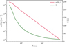 |
Fig. D.2 H2 density (left-hand y-axis) and kinetic temperature (Tgas = Tdust; right-hand y-axis) as a function of distance from the centre in the IRAS16293-2422 model (from Crimier et al. 2010). |
The chemical simulations in the protostellar stage are carried out by selecting a set of points along the physical model profiles and running the chemical simulation separately for each of the selected points, taking the initial abundances obtained from the preceding dark cloud simulation. This very simple model setup hence neglects any physical evolution between the dark cloud and protostellar core stages, and assumes that the initial chemical conditions are equal across the protostellar core. While such an approach is certainly not realistic, it does allow us to obtain rough estimates of the gas-phase and ice 12C/13C abundance ratios across the protostellar core. Naturally, the simulation results are also in this case sensitive to the choice of evolutionary time when the abundances are extracted from the model output. We chose here an early time of 104 yr to reflect the fact that the physical model is not describing well the very inner regions of the core where substructure has already formed.
References
- Agúndez, M., Marcelino, N., Cernicharo, J., Roueff, E., & Tafalla, M. 2019, A&A, 625, A147 [Google Scholar]
- Allen, V., van der Tak, F. F. S., Sánchez-Monge, Á., Cesaroni, R., & Beltrán, M. T. 2017, A&A, 603, A133 [NASA ADS] [CrossRef] [EDP Sciences] [Google Scholar]
- Belloche, A., Maury, A. J., Maret, S., et al. 2020, A&A, 635, A198 [NASA ADS] [CrossRef] [EDP Sciences] [Google Scholar]
- Beltrán, M. T., Cesaroni, R., Rivilla, V. M., et al. 2018, A&A, 615, A141 [Google Scholar]
- Bergin, E. A., Bosman, A., Teague, R., et al. 2024, ApJ, 965, 147 [NASA ADS] [CrossRef] [Google Scholar]
- Bouscasse, L., Csengeri, T., Belloche, A., et al. 2022, A&A, 662, A32 [NASA ADS] [CrossRef] [EDP Sciences] [Google Scholar]
- Bouscasse, L., Csengeri, T., Wyrowski, F., Menten, K. M., & Bontemps, S. 2024, A&A, 686, A252 [NASA ADS] [CrossRef] [EDP Sciences] [Google Scholar]
- Brunken, N. G. C., van Dishoeck, E. F., Slavicinska, K., et al. 2024, A&A, 692, A163 [NASA ADS] [CrossRef] [EDP Sciences] [Google Scholar]
- Brünken, S., Sipilä, O., Chambers, E. T., et al. 2014, Nature, 516, 219 [Google Scholar]
- Busch, L. A., Belloche, A., Garrod, R. T., Müller, H. S. P., & Menten, K. M. 2022, A&A, 665, A96 [NASA ADS] [CrossRef] [EDP Sciences] [Google Scholar]
- Busch, L. A., Belloche, A., Garrod, R. T., Müller, H. S. P., & Menten, K. M. 2024, A&A, 681, A104 [NASA ADS] [CrossRef] [EDP Sciences] [Google Scholar]
- Calcutt, H., Jørgensen, J. K., Müller, H. S. P., et al. 2018, A&A, 616, A90 [NASA ADS] [CrossRef] [EDP Sciences] [Google Scholar]
- Caselli, P., & Ceccarelli, C. 2012, A&A Rev., 20, 56 [NASA ADS] [CrossRef] [Google Scholar]
- Ceccarelli, C., Caselli, P., Bockelée-Morvan, D., et al. 2014, in Protostars and Planets VI, eds. H. Beuther, R. S. Klessen, C. P. Dullemond, & T. Henning, 859 [Google Scholar]
- Chen, Y., Rocha, W. R. M., van Dishoeck, E. F., et al. 2024, A&A, 690, A205 [NASA ADS] [CrossRef] [EDP Sciences] [Google Scholar]
- Cleeves, L. I., Bergin, E. A., Alexander, C. M. O. D., et al. 2014, Science, 345, 1590 [NASA ADS] [CrossRef] [Google Scholar]
- Colzi, L., Sipilä, O., Roueff, E., Caselli, P., & Fontani, F. 2020, A&A, 640, A51 [NASA ADS] [CrossRef] [EDP Sciences] [Google Scholar]
- Crimier, N., Ceccarelli, C., Maret, S., et al. 2010, A&A, 519, A65 [NASA ADS] [CrossRef] [EDP Sciences] [Google Scholar]
- Csengeri, T., Belloche, A., Bontemps, S., et al. 2019, A&A, 632, A57 [NASA ADS] [CrossRef] [EDP Sciences] [Google Scholar]
- Daniel, F., Gérin, M., Roueff, E., et al. 2013, A&A, 560, A3 [NASA ADS] [CrossRef] [EDP Sciences] [Google Scholar]
- De Simone, M., Ceccarelli, C., Codella, C., et al. 2020, ApJ, 896, L3 [NASA ADS] [CrossRef] [Google Scholar]
- Drozdovskaya, M. N., Schroeder I, I. R. H. G., Rubin, M., et al. 2021, MNRAS, 500, 4901 [Google Scholar]
- Dutta, S., Lee, C.-F., Liu, T., et al. 2020, ApJS, 251, 20 [NASA ADS] [CrossRef] [Google Scholar]
- Endres, C. P., Schlemmer, S., Schilke, P., Stutzki, J., & Müller, H. S. P. 2016, J. Mol. Spectrosc., 327, 95 [NASA ADS] [CrossRef] [Google Scholar]
- Fisher, J., Paciga, G., Xu, L.-H., et al. 2007, J. Mol. Spectrosc., 245, 7 [NASA ADS] [CrossRef] [Google Scholar]
- Franceschi, R., Henning, T., Smirnov-Pinchukov, G. V., et al. 2024, A&A, 687, A174 [NASA ADS] [CrossRef] [EDP Sciences] [Google Scholar]
- Gandhi, S., de Regt, S., Snellen, I., et al. 2023, ApJ, 957, L36 [NASA ADS] [CrossRef] [Google Scholar]
- Garrod, R. T., Jin, M., Matis, K. A., et al. 2022, ApJS, 259, 1 [NASA ADS] [CrossRef] [Google Scholar]
- Giani, L., Ceccarelli, C., Mancini, L., et al. 2023, MNRAS, 526, 4535 [NASA ADS] [CrossRef] [Google Scholar]
- Gieser, C., Pineda, J. E., Segura-Cox, D. M., et al. 2024, A&A, 692, A55 [NASA ADS] [CrossRef] [EDP Sciences] [Google Scholar]
- Goldsmith, P. F., & Langer, W. D. 1999, ApJ, 517, 209 [Google Scholar]
- Harju, J., Sipilä, O., Brünken, S., et al. 2017, ApJ, 840, 63 [NASA ADS] [CrossRef] [Google Scholar]
- Hily-Blant, P., Magalhaes de Souza, V., Kastner, J., & Forveille, T. 2019, A&A, 632, L12 [NASA ADS] [CrossRef] [EDP Sciences] [Google Scholar]
- Hsu, S.-Y., Liu, S.-Y., Liu, T., et al. 2020, ApJ, 898, 107 [Google Scholar]
- Hsu, S.-Y., Liu, S.-Y., Liu, T., et al. 2022, ApJ, 927, 218 [NASA ADS] [CrossRef] [Google Scholar]
- Hsieh, T. H., Segura-Cox, D. M., Pineda, J. E., et al. 2023, A&A, 669, A137 [NASA ADS] [CrossRef] [EDP Sciences] [Google Scholar]
- Hsieh, T. H., Pineda, J. E., Segura-Cox, D. M., et al. 2024, A&A, 686, A289 [NASA ADS] [CrossRef] [EDP Sciences] [Google Scholar]
- Hsieh, T. H., Pineda, J. E., Segura-Cox, D. M., et al. 2025, A&A, 696, A1 [NASA ADS] [CrossRef] [EDP Sciences] [Google Scholar]
- Ibrahim, M., Guillemin, J.-C., Chaquin, P., Markovits, A., & Krim, L. 2022, Phys. Chem. Chem. Phys. (Incorp. Faraday Trans.), 24, 23245 [Google Scholar]
- Ichimura, R., Nomura, H., & Furuya, K. 2024, ApJ, 970, 55 [Google Scholar]
- Jensen, S., Spezzano, S., Caselli, P., et al. 2024, A&A, 685, A149 [NASA ADS] [CrossRef] [EDP Sciences] [Google Scholar]
- Jeong, J.-H., Lee, J.-E., Lee, S., et al. 2025, ApJS, 276, 49 [Google Scholar]
- Jørgensen, J. K., Kuruwita, R. L., Harsono, D., et al. 2022, Nature, 606, 272 [CrossRef] [Google Scholar]
- Jørgensen, J. K., van der Wiel, M. H. D., Coutens, A., et al. 2016, A&A, 595, A117 [Google Scholar]
- Jørgensen, J. K., Müller, H. S. P., Calcutt, H., et al. 2018, A&A, 620, A170 [Google Scholar]
- Langer, W. D., Graedel, T. E., Frerking, M. A., & Armentrout, P. B. 1984, ApJ, 277, 581 [Google Scholar]
- Lee, S., Nomura, H., & Furuya, K. 2024, ApJ, 969, 41 [NASA ADS] [CrossRef] [Google Scholar]
- Line, M. R., Brogi, M., Bean, J. L., et al. 2021, Nature, 598, 580 [NASA ADS] [CrossRef] [Google Scholar]
- Loison, J.-C., Wakelam, V., Gratier, P., et al. 2019, MNRAS, 485, 5777 [Google Scholar]
- Loison, J.-C., Wakelam, V., Gratier, P., & Hickson, K. M. 2020, MNRAS, 498, 4663 [Google Scholar]
- Magalhäes, V. S., Hily-Blant, P., Faure, A., Hernandez-Vera, M., & Lique, F. 2018, A&A, 615, A52 [NASA ADS] [CrossRef] [EDP Sciences] [Google Scholar]
- Mangum, J. G., & Shirley, Y. L. 2015, PASP, 127, 266 [Google Scholar]
- Manigand, S., Jørgensen, J. K., Calcutt, H., et al. 2020, A&A, 635, A48 [NASA ADS] [CrossRef] [EDP Sciences] [Google Scholar]
- Maret, S., Hily-Blant, P., Pety, J., Bardeau, S., & Reynier, E. 2011, A&A, 526, A47 [NASA ADS] [CrossRef] [EDP Sciences] [Google Scholar]
- Milam, S. N., Savage, C., Brewster, M. A., Ziurys, L. M., & Wyckoff, S. 2005, ApJ, 634, 1126 [Google Scholar]
- Müller, H. S. P., Drouin, B. J., & Pearson, J. C. 2009, A&A, 506, 1487 [NASA ADS] [CrossRef] [EDP Sciences] [Google Scholar]
- Müller, H. S. P., Brown, L. R., Drouin, B. J., et al. 2015, J. Mol. Spectrosc., 312, 22 [CrossRef] [Google Scholar]
- Nazari, P., Tabone, B., van’t Hoff, M. L. R., Jørgensen, J. K., & van Dishoeck, E. F. 2023, ApJ, 951, L38 [NASA ADS] [CrossRef] [Google Scholar]
- Nomura, H., Furuya, K., Cordiner, M. A., et al. 2023, in Astronomical Society of the Pacific Conference Series, 534, Protostars and Planets VII, eds. S. Inutsuka, Y. Aikawa, T. Muto, K. Tomida, & M. Tamura, 1075 [Google Scholar]
- Pagani, L., Bergin, E., Goldsmith, P. F., et al. 2019, A&A, 624, L5 [NASA ADS] [CrossRef] [EDP Sciences] [Google Scholar]
- Palau, A., Walsh, C., Sánchez-Monge, Á., et al. 2017, MNRAS, 467, 2723 [NASA ADS] [Google Scholar]
- Piétu, V., Dutrey, A., & Guilloteau, S. 2007, A&A, 467, 163 [Google Scholar]
- Pineda, J. E., Sipilä, O., Segura-Cox, D. M., et al. 2024, A&A, 686, A162 [NASA ADS] [CrossRef] [EDP Sciences] [Google Scholar]
- Podio, L., Tabone, B., Codella, C., et al. 2021, A&A, 648, A45 [NASA ADS] [CrossRef] [EDP Sciences] [Google Scholar]
- Rampinelli, L., Facchini, S., Leemker, M., et al. 2025, A&A, 698, A115 [NASA ADS] [CrossRef] [EDP Sciences] [Google Scholar]
- Romano, D. 2022, A&A Rev., 30, 7 [NASA ADS] [CrossRef] [Google Scholar]
- Roueff, E., Loison, J. C., & Hickson, K. M. 2015, A&A, 576, A99 [NASA ADS] [CrossRef] [EDP Sciences] [Google Scholar]
- Sakai, N., Ceccarelli, C., Bottinelli, S., Sakai, T., & Yamamoto, S. 2012, ApJ, 754, 70 [NASA ADS] [CrossRef] [Google Scholar]
- Semenov, D., Henning, T., Guilloteau, S., et al. 2024, A&A, 685, A126 [NASA ADS] [CrossRef] [EDP Sciences] [Google Scholar]
- Sipilä, O., Caselli, P., & Harju, J. 2015, A&A, 578, A55 [Google Scholar]
- Sipilä, O., Colzi, L., Roueff, E., et al. 2023, A&A, 678, A120 [NASA ADS] [CrossRef] [EDP Sciences] [Google Scholar]
- Tobin, J. J., Looney, L. W., Li, Z.-Y., et al. 2016, ApJ, 818, 73 [CrossRef] [Google Scholar]
- Valdivia-Mena, M. T., Pineda, J. E., Segura-Cox, D. M., et al. 2022, A&A, 667, A12 [NASA ADS] [CrossRef] [EDP Sciences] [Google Scholar]
- Valdivia-Mena, M. T., Pineda, J. E., Caselli, P., et al. 2024, A&A, 687, A71 [NASA ADS] [CrossRef] [EDP Sciences] [Google Scholar]
- van Gelder, M. L., Tabone, B., Tychoniec, L·., et al. 2020, A&A, 639, A87 [NASA ADS] [CrossRef] [EDP Sciences] [Google Scholar]
- van Gelder, M. L., Nazari, P., Tabone, B., et al. 2022, A&A, 662, A67 [NASA ADS] [CrossRef] [EDP Sciences] [Google Scholar]
- van’t Hoff, M. L. R., Bergin, E. A., Jørgensen, J. K., & Blake, G. A. 2020, ApJ, 897, L38 [CrossRef] [Google Scholar]
- van’t Hoff, M.L. R., Bergin, E. A., Riley, P., et al. 2024, ApJ, 970, 138 [Google Scholar]
- Visser, R., van Dishoeck, E. F., & Black, J. H. 2009, A&A, 503, 323 [NASA ADS] [CrossRef] [EDP Sciences] [Google Scholar]
- Wampfler, S. F., Jørgensen, J. K., Bizzarro, M., & Bisschop, S. E. 2014, A&A, 572, A24 [NASA ADS] [CrossRef] [EDP Sciences] [Google Scholar]
- Widicus Weaver, S. L., Laas, J. C., Zou, L., et al. 2017, ApJS, 232, 3 [NASA ADS] [CrossRef] [Google Scholar]
- Wilson, T. L. 1999, Rep. Progr. Phys., 62, 143 [CrossRef] [Google Scholar]
- Xu, L.-H., & Lovas, F. J. 1997, J. Phys. Chem. Ref. Data, 26, 17 [Google Scholar]
- Xu, L.-H., Fisher, J., Lees, R. M., et al. 2008, J. Mol. Spectrosc., 251, 305 [NASA ADS] [CrossRef] [Google Scholar]
- Yamato, Y., Notsu, S., Aikawa, Y., et al. 2024, AJ, 167, 66 [NASA ADS] [CrossRef] [Google Scholar]
- Yang, Y.-L., Sakai, N., Zhang, Y., et al. 2021, ApJ, 910, 20 [Google Scholar]
- Yoshida, K., Sakai, N., Nishimura, Y., et al. 2019, PASJ, 71, S18 [NASA ADS] [CrossRef] [Google Scholar]
- Yoshida, T. C., Nomura, H., Furuya, K., Tsukagoshi, T., & Lee, S. 2022, ApJ, 932, 126 [NASA ADS] [CrossRef] [Google Scholar]
- Yoshida, T. C., Nomura, H., Furuya, K., et al. 2024, ApJ, 966, 63 [Google Scholar]
- Zhang, K., Bergin, E. A., Blake, G. A., Cleeves, L. I., & Schwarz, K. R. 2017, Nat. Astron., 1, 0130 [NASA ADS] [CrossRef] [Google Scholar]
- Zhang, Y., Snellen, I. A. G., Bohn, A. J., et al. 2021, Nature, 595, 370 [NASA ADS] [CrossRef] [Google Scholar]
- Zucker, C., Schlafly, E. F., Speagle, J. S., et al. 2018, ApJ, 869, 83 [NASA ADS] [CrossRef] [Google Scholar]
Lower 12C/13C ratios than expected have also been found towards high-mass analogues (e.g. Palau et al. 2017; Beltrán et al. 2018; Bouscasse et al. 2022). These results are not discussed in the current work, as we focus on low-mass protostellar objects.
When the mass number of the C atom is not specified, we talk about the main isotope 12C.
Entries for CH3CN isotopologues use spectroscopic data from Müller et al. (2009, 2015), for CH3OH from Xu et al. (2008), for 13CH3OH from Xu & Lovas (1997), and for CH318OH from Fisher et al. (2007).
We tested the effect of a factor of 10 variations in the cosmic-ray ionisation rate, similar to the range reported by Pineda et al. (2024), but the results were not significantly different to those of the fiducial model, and are hence not shown here.
All Tables
List of sources from the PRODIGE sample towards which 13C isotopologues of CH3 OH and CH3 CN have been detected.
Column density ratios for CH3 OH and CH3 CN isotopologues derived from the Weeds models.
All Figures
|
Fig. 1 Literature 12C/13C ratios towards sources at different evolutionary stages using different isotopologues. Simple O- and N-bearing species (<6 atoms) share a light blue and light yellow colour, respectively, but have different markers. Black rectangles around the orange triangle (N) and coloured circles (O) indicate complex organics (>6 atoms). Arrows indicate lower limits. References to the values can be found in Table A.9. |
| In the text | |
|
Fig. 2 Overview of the PRODIGE data towards IRAS 4B and presentation of the spectral line analyses. Panel a: integrated intensity map for th CH3CN 123−113 transition at 220.708 GHz. The beam (half power beam width, HPBW) is shown in the bottom left. The dashed yellow contou is at 5σ, where σ is the rms noise level and is written in the top-right corner. Panel b: observed spectra towards the peak position, which is a (Δα, Δβ = (0″, 0″) (black cross in panel a), of CH3CN at low (~2 MHz, black) and high (~62.5 kHz, teal) spectral resolution, where the latte] was shifted by 4K for visualisation. The low spectral-resolution data were analysed in this work (see Sect. 3). The modelled CH3CN spectra from Weeds are shown in red (low resolution) and orange (high resolution), where the same input parameters were used for both. Panel c: population diagram for CH3CN. Teal circles show the observed data points while the modelled data points from Weeds are shown with orange squares (se Sect. 4.6 for possible origins of differences between the two). No corrections are applied in the left panel, while in the right panel, corrections fo opacity and contamination by other molecules have been considered (negligible effect in this case), and only transitions with optical depths <0.5 (i.e. all transitions in this case) are shown. The results of the linear fit to the observed data points are shown in the right panels. |
| In the text | |
|
Fig. 3 Peak velocity, νpeak, and line width, FWHM, derived from 1D Gaussian fits (including 1σ error bars) to the high spectral-resolution (HR) PRODIGE data as a function of upper-level energy, Eu, for the vibrational ground states of CH3 OH (orange) and 13CH3OH (teal). The coloured dashed lines indicate the respective average values for νpeak and FWHM. |
| In the text | |
|
Fig. 4 Rotational temperatures used for the Weeds modelling (crosses) and derived from the population diagrams (circles with 1σ error bars). The dashed lines indicate the median values considering all isotopologues of a species. |
| In the text | |
|
Fig. 5 Same as Fig. 1 but including the 12C/13C ratios derived from the PRODIGE data in this work (light red shaded). Bolometric luminosities of the protostars increase from left to right. Black rectangles around markers indicate complex organic molecules. Arrows indicate lower limits. |
| In the text | |
|
Fig. 6 Column density ratio between 13CH3OH and CH318OH using the Weeds column densities. The expected local ISM value of ~8 is indicated with a dashed line. Arrows show lower limits. |
| In the text | |
|
Fig. 7 Model predictions for selected gas-phase 12C/13C ratios as a function of distance from the protostar taken at a simulation time of 104 yr. The constant ratio of 68 is indicated by the horizontal dashed black line. The vertical dotted black line separates the spatial scales discussed in this paper (R < 300 au) from the larger scales, which are not largely discussed but shown for completeness. |
| In the text | |
|
Fig. B.1 Integrated intensity maps using two transitions for both isotopologues of CH3 OH, the main CH3CN isotopologue, and one transition for each of the 13C isotopologue towards IRAS 2A. Respective rest frequencies (in GHz) are shown in the bottom-right corner, the beam (half power beam width, HPBW) on the bottom left. Multiplication factors (e.g. ×3, next to the species name) were applied to some species and transitions to be able to use the same intensity scale for all panels. The yellow dashed contour is at 5σ, where σ is the rms noise level (in K km s−1) and is written in the top-right corner. |
| In the text | |
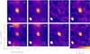 |
Fig. B.2 Same as Fig. B.1 but for IRAS 4B. |
| In the text | |
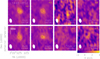 |
Fig. B.3 Same as Fig. B.1 but for L1448-IRS2. |
| In the text | |
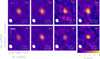 |
Fig. B.4 Same as Fig. B.1 but for B1-c. |
| In the text | |
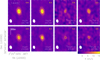 |
Fig. B.5 Same as Fig. B.1 but for L1448C. |
| In the text | |
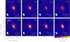 |
Fig. B.6 Same as Fig. B.1 but for SVS13A. |
| In the text | |
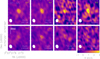 |
Fig. B.7 Same as Fig. B.1 but for B1-bS. |
| In the text | |
|
Fig. C.1 Population diagrams for CH3 OH, 13CH3OH, CH3CN, 13CH3CN, and CH313CN towards IRAS 4B. Observed data points are shown with teal circles as indicated in the top-right corner of the left panel while the modelled data points from Weeds are shown as orange squares. No corrections are applied in the left panels while in the right panels corrections for opacity and contamination by other molecules have been considered for the observed and modelled populations. The results of the linear fit to the observed data points are shown in the right panels. |
| In the text | |
|
Fig. C.2 Same as C.1 but for L1448C. |
| In the text | |
|
Fig. C.3 Same as C.1 but for L1448-IRS2. |
| In the text | |
|
Fig. C.4 Same as C.1 but for B1-c. |
| In the text | |
|
Fig. C.5 Same as C.1 but for B1-bS. |
| In the text | |
|
Fig. C.6 Same as C.1 but for IRAS 2A. |
| In the text | |
|
Fig. C.7 Same as C.1 but for SVS13A. |
| In the text | |
|
Fig. C.8 Same as C.1 but for CH318OH towards IRAS 2A, IRAS 4B, SVS13A, and B1-c. |
| In the text | |
|
Fig. D.1 Model predictions for selected gas-phase and ice 12C/13C ratios as a function of time in the first simulation stage, representing evolution in dark cloud conditions. |
| In the text | |
|
Fig. D.2 H2 density (left-hand y-axis) and kinetic temperature (Tgas = Tdust; right-hand y-axis) as a function of distance from the centre in the IRAS16293-2422 model (from Crimier et al. 2010). |
| In the text | |
Current usage metrics show cumulative count of Article Views (full-text article views including HTML views, PDF and ePub downloads, according to the available data) and Abstracts Views on Vision4Press platform.
Data correspond to usage on the plateform after 2015. The current usage metrics is available 48-96 hours after online publication and is updated daily on week days.
Initial download of the metrics may take a while.