| Issue |
A&A
Volume 699, July 2025
|
|
|---|---|---|
| Article Number | A184 | |
| Number of page(s) | 16 | |
| Section | Extragalactic astronomy | |
| DOI | https://doi.org/10.1051/0004-6361/202553693 | |
| Published online | 04 July 2025 | |
The impact of morphological quenching mechanisms on star formation activity at 0.2 < z < 1.2 in the COSMOS field
1
School of Mathematics and Physics, Anqing Normal University, Anqing, 246133
China
2
Institute of Astronomy and Astrophysics, Anqing Normal University, Anqing, 246133
China
3
Key Laboratory of Modern Astronomy and Astrophysics (Nanjing University), Ministry of Education, Nanjing, 210093
China
4
Department of Physics, The Chinese University of Hong Kong, Shatin N.T., Hong Kong S.A.R., China
⋆ Corresponding authors: This email address is being protected from spambots. You need JavaScript enabled to view it.
, This email address is being protected from spambots. You need JavaScript enabled to view it.
Received:
7
January
2025
Accepted:
27
May
2025
Abstract
The distribution of galaxies in the color-magnitude diagram (CMD) reveals two distinct groups: the red sequence and the blue cloud, along with an intermediate region known as the green valley (GV), which is considered an important transitional stage in galaxy evolution. Examining the difference in morphology and environment of GV galaxies with early-type disks (ETDs: bulge-dominated and with a disk) and late-type disks (LTDs: disk-dominated) could help improve our understanding of the corresponding quenching mechanisms. Based on the COSMOS2020 catalog, we selected a large sample of massive (M* ≥ 1010 M⊙) GV galaxies at 0.2 < z < 1.2 by using the extinction-corrected (U − V)rest colors. After excluding the possible active galactic nucleus candidates and applying the criterion of “mass-matching”, two subsamples of GV galaxies were ultimately constructed at 0.2 < z < 0.7 (457 ETDs and 457 LTDs) and 0.7 ≤ z < 1.2 (839 ETDs and 839 LTDs), respectively. Compared to LTDs, we find that ETDs present higher Gini coefficients and concentration C, more negative M20 values, and lower specific star formation rates (sSFRs); whereas ETDs possess more concentrated profiles, but there is no significant difference in terms of environment between ETDs and LTDs. These results indicate that the morphological effect could probably play an important role in quenching the star formation activity of massive GV galaxies instead of the environmental effect. Additionally, we employed a dimensionless parameter morphology quenching efficiency (Qmor) to quantify the connection between galaxy morphology and star formation activity. We find that Qmor is relatively sensitive to stellar mass than redshifts, especially for massive galaxies with M* > 1010.8 M⊙ at z < 1. The probability of Qmor ≥ 0.15 approaches ∼75% when the discrepancy of average star formation rates between ETDs and LTDs is approximately 0.3 M⊙ yr−1. The Qmor ≥ 0.15 could probably be used to characterize the level of morphological quenching in GV galaxies, which is more pronounced in massive (M* ≥ 1010.8 M⊙) galaxies.
Key words: stars: formation / Galaxy: evolution / Galaxy: structure
© The Authors 2025
 Open Access article, published by EDP Sciences, under the terms of the Creative Commons Attribution License (https://creativecommons.org/licenses/by/4.0), which permits unrestricted use, distribution, and reproduction in any medium, provided the original work is properly cited.
This article is published in open access under the Subscribe to Open model. This email address is being protected from spambots. You need JavaScript enabled to view it. to support open access publication.
1. Introduction
With advancements in high-quality, all-sky galaxy surveys, numerous studies have revealed that galaxies on the color-magnitude diagram (CMD) primarily fall into two distinct populations, including the red sequence (RS) and the blue cloud (BC; e.g., Baldry et al. 2004; Salim 2014; Angthopo et al. 2020; Corcho-Caballero et al. 2021). The former one is dominated by red galaxies, which are typically gas-poor systems with little ongoing star formation activity. In contrast, the latter one is populated by blue galaxies, characterized by active star formation and abundant gas content. Separating these two regions is the green valley (GV), a sparsely populated area thought to represent a crucial transitional phase in galaxy evolution (e.g., Wyder et al. 2007; Gu et al. 2018).
Many previous studies have revealed that galaxies may undergo the GV through different evolutionary pathways (e.g., Salim 2014; Schawinski et al. 2014; Smith et al. 2022). On the one hand, GV galaxies may suppress star formation by transitioning from BC to RS via different mechanisms (Gu et al. 2018; Sampaio et al. 2023), such as the internal active galactic nucleus (AGN) feedback or the external environment. Sampaio et al. (2023) investigated the impact of AGN feedback on galaxy evolution using a sample of 80 000 central galaxies from the Solan Digital Sky Survey (SDSS). They found that the fraction of AGNs increases as star formation activity declines in the BC, peaking near the GV (∼17 ± 4%) and then decreasing as galaxies transition to the RS. Thus, the AGN feedback in GV galaxies plays a critical role in regulating and suppressing star formation. Based on the survey in the five 3D-HST/CANDELS fields, Gu et al. (2018) explored the environment of GV galaxies at 0.5 < z < 2.5, compared to BC and RS galaxies. They found a significant environmental difference between GV and RS galaxies at z < 1.5, which is consistent with results of Schawinski et al. (2007), where more early-type galaxies are found in the GV. Gu et al. (2018) also pointed out the highest AGN fraction in GV galaxies at z < 2, which reconciles with Sampaio et al. (2023). On the other hand, not all GV galaxies follow the above evolutionary sequence from BC to RS. Some studies suggested that GV galaxies might come from RS galaxies by rejuvenation events, such as gas accretion from the intergalactic medium (IGM; Thilker et al. 2010). Salim et al. (2012) suggested that galaxies could move between the state with low star formation and the quiescent state due to the impact of the duty cycle (Type 2) AGN, which was also supported by the results from Fang et al. (2012, 2013).
Morphological studies found that there is a different structure between GV, BC, and RS galaxies (e.g., Fang et al. 2013; Gu et al. 2018). The GV galaxies share the structural and characteristic features with both RS and BC galaxies (Gu et al. 2018; Smith et al. 2022). Smith et al. (2022) found that ring structures more commonly appear in the GV galaxies, resulting from fading discs. They noted that the evolutionary pathway from BC to RS reconciles with the loosening spiral-arm structure. The prominence of the central bulge grows steadily from BC to RS, with GV galaxies exhibiting an intermediate state, which was also found by Pandya et al. (2017) and Gu et al. (2018). Based on the Mapping Nearby Galaxies at APO (MaNGA) MPL-5 survey, Cano-Díaz et al. (2019) explored the dependence of global or local (spatially resolved) star-forming main sequences on galaxy morphology. They found that the area with lower star formation tends to have earlier morphological types, emphasizing the regulatory role of morphology in the star formation process. Martig et al. (2009) proposed morphological quenching (MQ) as a significant mechanism behind the suppression of star formation, which acts by leveraging the structural characteristics and gravitational potential distribution of galaxies. The prominent central bulge of a galaxy creates a concentrated mass distribution that stabilizes the gas disk through its gravitational potential (Su et al. 2019; Gensior et al. 2020). This stabilization reduces gas fragmentation and ultimately inhibits star formation. Unlike traditional quenching mechanisms, which remove cold gas reservoirs (e.g., Cortese et al. 2021; Wright et al. 2022) or halt gas inflows (Rasmussen et al. 2006), MQ operates through the galaxy’s internal evolutionary processes. Observational studies have provided evidence supporting MQ as an effective mechanism for galaxy quenching (e.g., Bundy et al. 2010; Bluck et al. 2014; Dimauro et al. 2022). For example, many local red early-type galaxies have been found to retain high-density molecular or atomic gas, yet exhibit little to no significant star formation activity (e.g., Crocker et al. 2011; Su et al. 2015; Ruffa & Davis 2024). This phenomenon can be explained by the stabilizing effect of the bulge’s gravitational potential on the gas, without requiring an external feedback mechanism.
The GV galaxy sample is probably the ideal laboratory to explore the morphological transitions of early-type galaxies and late-type galaxies at a comparable evolutionary stage. At higher redshifts, the morphological evolution of galaxies is often obscured by complex processes such as rapid star formation, mergers, and gas accretion (Bournaud & Elmegreen 2009). However, galaxies exhibit clearer morphological features at intermediate to low redshifts, making it easier to study these transitions. Gu et al. (2018) pointed out that GV galaxies have a rapidly increasing distribution of Sérsic index at z < 1.5, which suggests that the intermediate redshift range could offer a unique opportunity to evaluate the impact of morphology on star formation quenching. To explore the true impact of the MQ mechanism on star formation activity, we utilized the extinction-corrected rest-frame U − V color (Wang et al. 2017) to construct a sample of massive (M* ≥ 1010 M⊙) GV galaxies in the COSMOS2020 catalog at 0.2 < z < 1.2. Since the star formation rate density of the Universe decreases after cosmic noon (Madau & Dickinson 2014) and the influence of the environment on star formation begins to appear at 0.2 < z < 1.1 (Jian et al. 2018), focusing on GV galaxies in this redshift range could be suitable for exploring the dominated quenching mechanisms of galaxy evolution. After excluding the influence of AGN as much as possible, we further divided the GV galaxy sample into two types of galaxies: early-type disk (ETD) and late-type disk (LTD), based on the apt classification of galaxy morphologies from Song et al. (2024). Then, we compared the distributions of nonparametric structure (Gini versus M20 and C), the specific star formation rate (sSFR), the morphological quenching efficiency (Qmor), the radial surface brightness, and the surrounding environment for ETD galaxies (hereafter, ETDs) and LTD galaxies (hereafter, LTDs), aiming to elucidate the impact of MQ on star formation activity gradually.
The structure of this work is as follows. Section 2 provides a detailed overview of the dataset and the sample selection of GV galaxies. In Sect. 3, we analyze the MQ of star formation activity in GV galaxies by comparisons of nonparametric structure in Sect. 3.1, sSFR in Sect. 3.2, the MQ efficiency in Sect. 3.3, the radial surface brightness in Sect. 3.4, and the environmental effects in Sect. 3.5, to investigate the impact of MQ on star formation activity in ETDs and LTDs. The discussion is presented in Sect. 4, followed by a summary in Sect. 5. Throughout this paper, we adopt the following cosmological parameters: H0 = 70 km s−1 Mpc−1, Ωm = 0.3, ΩΛ = 0.7. The AB magnitude is adopted in this work.
2. Data and sample selection
2.1. The COSMOS2020 catalog
The COSMOS field is devoted to the investigation of the intricate interrelationships between galaxy evolution, star formation, AGNs, dark matter, and large-scale structure, with a wide redshift range of 0.5 < z < 6, which covers an area of about 2 deg2 (Scoville et al. 2007; Hasinger et al. 2018). The sample utilized in this work is constructed from the “Farmer” COSMOS2020 catalog (Weaver et al. 2022), which provides comprehensive photometric data across 35 bands, ranging from ultraviolet to near-infrared (UV-NIR). Using this enhanced photometric dataset, Weaver et al. (2022) estimated various physical properties of galaxies within this field, including photometric redshifts and stellar masses, by fitting spectral energy distributions (SEDs) of galaxies.
To determine photometric redshifts, two independent codes were employed: EAZY (Brammer et al. 2008) and LePhare (Ilbert et al. 2006). For this analysis, we have chosen to utilize the redshifts obtained from LePhare, as their reliability, particularly within the relevant magnitude range, is evident in Figure 15 of Weaver et al. (2022). The process of estimating redshifts involved the use of a library containing 33 galaxy templates, derived from the models of Bruzual & Charlot (2003, BC03) and Ilbert et al. (2009). Furthermore, the analysis utilizes a variety of dust extinction and attenuation models, such as the starburst attenuation curve proposed by Calzetti et al. (2000), the SMC extinction curve from Prevot et al. (1984), and two modifications of the Calzetti et al. (2000) law, which include the 2175 Å absorption feature. The photometric redshift (zLePh) is ultimately defined as the median value extracted from the likelihood distribution of the redshift.
Following this, with the redshift fixed at zLePh, the LePhare fitting code was re-executed to derive stellar mass and other relevant physical properties. Besides the original libraries adopted in Ilbert et al. (2006), which include different types of galaxy templates (e.g., ellipticals, spirals, and blue star-forming galaxies), two additional templates for quiescent galaxies from BC03 with exponentially declining star formation rate (i.e., SFR ≈ e−t/τ) and a set of AGN (quasar) templates were employed as well to constrain redshifts and stellar masses better. More details are given in Laigle et al. (2016) and Weaver et al. (2022).
2.2. The morphological catalog
The morphology of a galaxy could be useful in conveying information about its formation and evolution (Guglielmo et al. 2015; Lee et al. 2024). The COSMOS field is an ideal survey to explore the morphology since ∼82% of the (∼2 deg2) COSMOS field was observed in the F184W (i.e., I band) filter by the Hubble Space Telescope (HST) with Advanced Camera for Surveys (ACS). Based on the high-resolution I band images with PSF = 0.095″ from HST/ACS in the COSMOS field, Song et al. (2024) constructed a morphological catalog of galaxies with Imag < 25 at 0.2 < z < 1.2 by refining a two-step galaxy morphological classification framework (USmorph), which combines the unsupervised machine-learning (UML) with the supervised machine-learning (SML) methods. They classified galaxies into five distinct types, including spherical (SPH), early-type disk (ETD), late-type disk (LTD), irregular disk (IRR), and unclassified (UNC). This work mainly focuses on two types of galaxies: ETDs and LTDs. Specifically, ETDs are dominated by bulges but also have a disk, while LTDs are dominated by disks. Both parametric and nonparametric morphological measurements of galaxies were conducted as well. The former includes the Sérsic index (n) and the effective radius (re), while the latter contains many coefficients, such as the Gini coefficient, the M20 index and the concentration C (see Sect. 3.1 for detailed definitions), as well as the other disk-related parameters, including the asymmetry, A, and clumpiness, S.
2.3. Star formation rates
In this work, the star formation rate (SFR) is estimated by combining the contributions from ultraviolet (UV) light, emitted by massive stars, and infrared (IR) emissions, which arise from dust-reprocessed light. Both UV and IR emissions are provided by Muzzin et al. (2013). Assuming a Chabrier (2003) initial mass function (IMF) and using the UV conversion from Bell et al. (2005), the total SFR is calculated via
![Mathematical equation: $$ \begin{aligned} \mathrm{SFR}_{\mathrm{UV+IR} } [M_\odot \,\mathrm{yr^{-1}}] = 1.09 \times 10^{-10} \times {(L_{\mathrm{IR} } + 2.2L_{\mathrm{UV} })}/{L_\odot }, \end{aligned} $$](/articles/aa/full_html/2025/07/aa53693-25/aa53693-25-eq1.gif) (1)
(1)
where LUV represents the integrated rest-frame UV (1216−3000 Å) luminosity. This is defined as 1.5 times the rest-frame monochromatic luminosity at 2800 Å, such that LUV = 1.5 × L2800. The IR luminosity, LIR, represents the integrated 8−1000 μm luminosity, converted from Spitzer/MIPS 24 μm data. If a 24 μm detection is unavailable, the SFR is corrected for dust attenuation (Av) using the dust attenuation curve from Calzetti et al. (2000) and
![Mathematical equation: $$ \begin{aligned} \mathrm{SFR}_{\mathrm{UV,corr} }[M_{\odot }\,\mathrm{yr^{-1}}] = \mathrm{SFR}_{\mathrm{UV} } \times 10^{0.4 \times 1.8 \times A_v}, \end{aligned} $$](/articles/aa/full_html/2025/07/aa53693-25/aa53693-25-eq2.gif) (2)
(2)
where the SFR based on the observed UV luminosity, denoted as SFRUV, is computed using the formula SFRUV [M⊙ yr−1] = 3.6 × 10⁻¹⁰ × L2800/L⊙, with the assumption of the Chabrier (2003) IMF, as outlined by Wuyts et al. (2011). Previous studies have confirmed the acceptable agreement between SFRUV, corr and SFRUV + IR (Wang et al. 2016; Gu et al. 2020).
2.4. Sample selection
2.4.1. The mass completeness limit
In this work, we cross-matched the “Farmer” COSMOS2020 catalog with the morphological catalog from Song et al. (2024) to obtain a parent sample. It includes about 99 806 galaxies, which already follow the following criteria: (1) Imag < 25, to exclude galaxies too faint for accurate morphological analysis; (2) the redshift at 0.2 < z < 1.2, ensuring that morphology is measured in the rest-frame optical; (3) FLAGCOMBINE = 0, which ensures that nearby bright stars do not contaminate flux measurements and that the objects are not located at the image edges, guaranteeing reliable photometric redshift and stellar mass estimates; (4) signal-to-noise ratios greater than 5 (i.e., S/N > 5), ensuring robust detections; (5) the flag of lptype = 0, to ensure the objects are galaxies rather than stars. The distribution of stellar mass (M*) as a function of redshift for this parent sample at 0.2 < z < 1.2 is shown in Fig. 1 with gray dots.
Since more massive galaxies can be detectable than low-mass galaxies as redshift increases due to the limitations in the observational depth and completeness, the sample variance could be strongly affected (Bates et al. 2019). To relieve this bias, we take the mass completeness of the parent sample into account by following the method described in Pozzetti et al. (2010). Specifically, we defined a minimum stellar mass (Mmin) at each redshift, above which the selected sample is generally completeness. To derive the Mmin, the limiting stellar mass (Mlim) of each galaxy needs to be estimated by log Mlim = log M* + 0.4(I − Ilim), which is the mass at a given redshift when the galaxy could be detected in a limited depth of the survey. We adopted the I band magnitude limit Ilim < 25 as the limiting magnitude of the COSMOS field with HST detections, which can be reconciled with the magnitude limit of the morphological catalog in Song et al. (2024). The Mlim can be derived from the 20% of faintest galaxies at given a redshift slice (Δz = 0.25). Then, the Mmin(z) can be defined as the upper bound of the Mlim distribution, where 95% of the Mlim values fall below this envelope at a given redshift. In Fig. 1, the thresholds of Mmin in four redshift intervals (Δz = 0.25) are shown in the green curve, while the solid black line presents the best fitting of them by the formula Mmin(z) = 1.28ln(z)+9.78. This Mmin can represent the ∼95% completeness limit. To ensure that the mass completeness of the entire parent sample is over 95% in the wide redshift range, we finally applied the threshold of stellar mass over 1010 M⊙ to the parent sample, as depicted by the dashed black line in Fig. 1. There are 19 457 galaxies singled out from the parent sample.
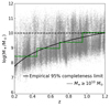 |
Fig. 1. Distribution of stellar mass as a function of redshift. The boundaries of mass completeness in different fixed redshift bins (Δz = 0.25) are shown in green. The solid black line represents the best fitting of boundaries by the parameterized function Mmin(z) = 1.28ln(z)+9.78. The mass threshold (M* = 1010 M⊙) adopted in this work is present in the dashed back line, which could ensure a ≥95% completeness up to z ∼ 1.2. The background gray dots represent the parent sample selected from the COSMOS2020 catalog (see Sect. 2.1). |
2.4.2. Green valley sample: ETDs and LTDs
To accurately construct the sample of GV galaxies, we applied the color-based separation criteria as outlined by Wang et al. (2017). This refined GV definition has been widely accepted by many previous studies (e.g., Gu et al. 2018, 2019; Lu et al. 2021; Chang et al. 2022) due to its high reliability. First, following the approach of Brammer et al. (2009), Wang et al. (2017) incorporated extinction correction (ΔAV = 0.47AV derived from Calzetti et al. 2000 attenuation law) to reduce the misclassification between quiescent and dusty star-forming galaxies, ensuring that the selected GV galaxies can reflect intrinsic stellar population properties rather than dust-obscured star-forming galaxies. Second, the mass- and redshift-dependent boundaries dynamically adapt to cosmic evolution trends, avoiding biases introduced by fixed color cuts. Third, the classification results do not change significantly when the GV boundaries are fine-tuned by ±0.1 mag (i.e., the extinction-corrected U − V colors are shifted by a small amount), indicating the good stability of this classification method. The criteria for distinguishing galaxies into BC, GV, and RS populations are as follows:
where ΔAV = 0.47AV denotes the extinction correction applied to the rest-frame U − V color. The GV galaxies are distributed between the two dividing lines, as shown by orange lines in Fig. 2. Since GV galaxies are considered the transition phase between the RS and BC population, which has been confirmed by many previous studies (e.g., Wang et al. 2017; Gu et al. 2018, 2019; Chang et al. 2022), as expected, we also find that the morphological parameters (including Gini, C, M20 and n) of GV galaxies distribute among RS and BC galaxies. Thus, we directly focus on the sample of 7930 GV galaxies with different morphologies. Based on the morphological classification from the catalog of Song et al. (2024), we further selected two types (ETD vs. LTD) of GV galaxies to explore the morphological effect on the galaxy star formation. The numbers of ETDs and LTDs are 2092 and 1370, respectively.
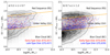 |
Fig. 2. Relationships between the extinction-corrected rest-frame U − V and stellar mass at 0.2 < z < 0.7 (left) and 0.7 ≤ z < 1.2 (right). The gray contours and mosaics in the background indicate the relative density in the color-mass panel. The criteria from Wang et al. (2017) was adopted to separate galaxies into RS, GV, and BC, respectively, as shown in orange lines in each panel. Based on the morphological classification from Song et al. (2024), the GV galaxies were further divided into two types, including early-type disk (ETD: red) and late-type disk (LTD: blue), separately. Both subsamples excluded the contamination from AGN candidates and considered the mass matching (see Sects. 2.4.2 and 2.4.3 for details). |
2.4.3. AGN removal and mass matching
To consider the impact of AGNs on galaxy morphology and avoid the complications of AGN feedback on the mechanisms affecting the star formation of GV galaxies, we aimed to exclude AGN candidates from our GV sample as thoroughly as possible. The mid-infrared (MIR) color criteria, recognized as a promising technique in numerous studies (e.g., Treyer et al. 2010; Satyapal et al. 2017; Sajina et al. 2022), has been widely adopted to identify obscured AGN candidates. Its efficacy is attributed to the fact that the MIR radiation is relativelyinsensitive to dust obscuration, making it capable of tracing the reprocessed emission from dust heated by the central nucleus.
Therefore, we adopted the MIR color criteria defined by Donley et al. (2012) to eliminate the 531 MIR AGN candidates from all GV galaxies. Specifically, we applied the following selection criteria in the IRAC color-color space:
where x = log10(f5.8 μm/f3.6 μm) and y = log10(f8.0 μm/f4.5 μm) and the IRAC flux is expected to follow the sequence of f3.6 μm < f4.5 μm < f5.8 μm < f8.0 μm. These criteria define a conservative selection wedge in the IRAC color-color space, tailored to identify sources with monotonically rising, power-law MIR spectral energy distributions, typical of AGN-dominated emission. Compared to previous MIR AGN selection methods, the criteria of Donley et al. (2012) significantly reduce contamination from star-forming galaxies, yielding a cleaner AGN sample with higher reliability. After excluding 531 MIR AGN candidates from the GV sample, we retained 809 ETDs and 457 LTDs at 0.2 < z < 0.7, and 1165 ETDs and 839 LTDs at 0.7 ≤ z < 1.2, respectively.
Additionally, to minimize the impact of stellar mass on the statistical analysis of galaxy morphology, we constructed a “mass-matched” sample of massive GV galaxies at 0.2 < z < 1.2. This approach could ensure that the selected ETDs and LTDs exhibit equivalent distributions in terms of the redshift and stellar mass. In accordance with the methodology outlined by Gu et al. (2019), the minimum count between the two populations is defined as the number of galaxies in the mass-matched sample at fixed redshift and stellar mass bins. Specifically, for each galaxy with coordinates (z0, M*, 0) in the ETDs, the corresponding LTD is selected based on the smallest value of  , ensuring the closest match in stellar mass. Consequently, our final sample comprises 457 ETDs and 457 LTDs at 0.2 < z < 0.7, and 839 ETDs and 839 LTDs at 0.7 ≤ z < 1.2, respectively. Figure 2 presents the extinction-corrected rest-frame color as a function of stellar mass. These ETDs and LTDs in the final sample are shown in red and blue dots, respectively. In this work, we have approximately two and seven times more cross-matched galaxies at 0.2 < z < 0.7 and 0.7 ≤ z < 1.2, respectively, than in Lu et al. (2021) at 0.5 < z < 1.0 (200 ETDs and 200 LTDs) and 1.0 ≤ z < 1.5 (119 ETDs and 119 LTDs); this is, of course, if the difference in the redshift interval is not taken into account.
3. Analysis
3.1. Non-parametric structure
Since nonparametric measurements of galaxy morphology do not assume a specific analytical function for the light distribution of galaxies, this is more suitable for our analysis of the selected samples. Since for disk-related parameters such as the asymmetry, A, and clumping, S, no differences have been found between ETDs and LTDs in the GV sample, we mainly focus on the Gini coefficient, the M20 index, and the concentration, C, in this work.
The Gini coefficient was initially introduced in economics to characterize wealth inequality within a population. Abraham et al. (2003) adapted this concept to describe the distribution of a galaxy’s flux. The corresponding metric is computed as follows:
 (3)
(3)
where Npix denotes the total number of pixels in the galaxy, where fi is the flux value of each pixel arranged in ascending order and  represents the average of all pixel flux values. A higher Gini value indicates that a galaxy’s light is concentrated in fewer pixels (i.e., more centrally concentrated), whereas a lower Gini value suggests a more uniform flux distribution across the galaxy.
The M20 index can represent the normalized second-order moment of the brightest 20% of a galaxy’s flux. It can reflect whether the light is concentrated within a single region of the galaxy. To calculate M20, galaxy pixels are first ranked in descending order by flux and the index is subsequently defined as:
 (4)
(4)
where ![Mathematical equation: $ M_{\mathrm{tot}}=\sum_i^{N_{\mathrm{pix}}}M_i=\sum_i^{N_{\mathrm{pix}}} f_i[(x_i-x_c)^2+(y_i-y_c)^2] $](/articles/aa/full_html/2025/07/aa53693-25/aa53693-25-eq9.gif) . Here, ftot is the total flux of the galaxy, fi is the flux value of each pixel, i, then (xi, yi) is the position of a pixel, i, and (xc, yc) is the center of the image. A more negative M20 value does not necessarily indicate that light is concentrated at the center; rather, it might be concentrated in various locations within the image. Lotz et al. (2004) used M20 to trace the spatial distribution of bright nuclei, bars, and off-center clusters. The Gini coefficient and M20 are often used together to classify galaxies into different morphological subclasses (Rodriguez-Gomez et al. 2019).
. Here, ftot is the total flux of the galaxy, fi is the flux value of each pixel, i, then (xi, yi) is the position of a pixel, i, and (xc, yc) is the center of the image. A more negative M20 value does not necessarily indicate that light is concentrated at the center; rather, it might be concentrated in various locations within the image. Lotz et al. (2004) used M20 to trace the spatial distribution of bright nuclei, bars, and off-center clusters. The Gini coefficient and M20 are often used together to classify galaxies into different morphological subclasses (Rodriguez-Gomez et al. 2019).
The concentration index (C) is a widely used morphological parameter that quantifies how centrally concentrated the light distribution of a galaxy is (e.g., Bershady et al. 2000; Conselice 2003). Following Conselice (2003), C can be estimated by the ratio of the radii enclosing 80% and 20% of the total flux, defined as:
 (5)
(5)
A higher value of C indicates that a larger fraction of the total light is confined to the central region of the galaxy, which is typical for elliptical or bulge-dominated systems; whereas the lower C values are commonly associated with disk galaxies or systems with low surface brightness.
In contrast, the asymmetry (A) and clumpiness (S) parameters are more sensitive to irregularities and clumpiness in galaxy disks that are typically associated with active star formation (Yesuf et al. 2021). We confirm that ETDs and LTDs have similar distributions in A and S, with tiny differences in their median values, indicating no significant distinction in their disk structures, which might be associated with a similar environment they inhabit (see Sect. 3.5). This differs from the results of Yesuf et al. (2021), where the symmetry (A) was identified as the most powerful structural parameter to predict star formation activity for local star-forming galaxies. Therefore, the bulge-related parameters play a more important role in regulating the star formation in the GV population.
Figure 3 presents the Gini-M20 (top panels) and Gini-C (bottom panels) distributions of ETDs (red) and LTDs (blue) within three different redshift bins. Regardless of stellar mass, ETDs generally exhibit higher Gini and C, and lower M20, compared to LTDs, indicating that the starlight in ETDs is more centrally concentrated and ETDs show more bulge-dominated structures. In addition, both ETDs and LTDs have higher Gini and C, and lower M20 values with increasing stellar mass. This implies that more massive galaxies tend to be concentrated, revealing that the stellar mass could play a crucial role in shaping galaxy morphology and driving morphological evolution. Figure 4 presents several I band images of ETDs (red) and LTDs (blue) at 0.2 < z < 0.7. More example images at 0.7 ≤ z < 1.2 are given in Appendix A. These images can also reveal that LTDs are predominantly disk-like, while ETDs are mainly bulge-dominated. This further supports the trend mentioned in Fig. 3.
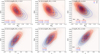 |
Fig. 3. Distributions of ETDs (red) and LTDs (blue) in the Gini-M20 (top panels) and Gini-C (bottom panels) spaces within three stellar mass bins (left: 10.0 ≤ log(M*/M⊙) < 10.4, middle: 10.4 ≤ log(M*/M⊙) < 10.8, right: log(M*/M⊙)≥10.8). The red (blue) background represents the number density distribution of ETDs (LTDs) in each space. The red (blue) contours enclose 30%, 50%, and 70% of the respective subsamples. The red (blue) diamond indicates the median value of ETDs (LTDs) in each space, with ±25th percentile uncertainties. The corresponding median values and uncertainties are displayed at the bottom of each panel. |
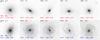 |
Fig. 4. Example images of ETDs (the first row) and LTDs (the second row) at 0.2 < z < 0.7 in the I band (see Fig. A.1 for example images at 0.7 ≤ z < 1.2). The corresponding information of each ETD (LTD) galaxy is depicted in red (blue) on the image, including the galaxy ID from the COSMOS2020 catalog, photometric redshift, Gini coefficient, M20 index, and the concentration, C. |
3.2. Specific star formation rate
The connection between the sSFR and galaxy morphology has been examined extensively in previous studies, revealing an inverse correlation between the sSFR of a galaxy and either its central mass concentration or the presence of a bulge (e.g., Bait et al. 2017; Koyama et al. 2019; Yesuf et al. 2021; Camps-Fariña et al. 2024). For instance, galaxies with prominent bulges or high central mass concentrations, such as early-type spirals, typically have lower sSFR than late-type spirals or irregular galaxies (Cook et al. 2020), indicating a strong link between bulges and star formation quenching. Therefore, we compared the sSFR distribution of ETDs with that of LTDs in three different stellar mass bins (i.e., 10.0 ≤ log(M*/M⊙) < 10.4, 10.4 ≤ log(M*/M⊙) < 10.8, and log(M*/M⊙)≥10.8) to assess whether the presence of a central bulge has a suppressive effect on sSFR due to morphological differences.
Figure 5 shows the relationship between sSFR and stellar mass of ETDs (red) and LTDs (blue) at 0.2 < z < 0.7 and 0.7 ≤ z < 1.2, respectively. To quantitatively assess the difference in sSFR between ETDs and LTDs, we performed a Mann-Whitney U-test for the difference in median values. The p-values of the U-test are 0.024 and 0.0004 at low- and high-redshift bins, respectively. In both cases, the p-values are less than 0.05, indicating that there are significant differences between the sSFRs of ETDs and LTDs, especially at high redshifts, due to more intense star formation occurring in theearlier Universe (Madau & Dickinson 2014). Regardless of the stellar mass, ETDs have lower sSFRs than LTDs, which is consistent with previous findings (Wuyts et al. 2011; Lu et al. 2021). This result may indicate that the presence of a central bulge suppresses star formation in galaxies. Moreover, we observe a ∼0.4 dex decline in star formation activity with increasing stellar mass for both ETDs and LTDs, particularly for massive ETDs and LTDs. This suggests that more massive GV galaxies might quench star formation earlier than low-mass ones, supporting the “downsizing” scenario, where the most massive galaxies were formed earliest and quenched their star formation earlier than less massive ones (Cowie et al. 1996).
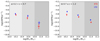 |
Fig. 5. Relation between sSFR and stellar mass for ETDs (red) and LTD (blue). Within each redshift bin, both ETDs and LTDs are separated into three stellar mass ranges: 10.0 ≤ log(M*/M⊙) < 10.4, 10.4 ≤ log(M*/M⊙) < 10.8, and log(M*/M⊙)≥10.8. The median values of the distributions for ETDs and LTDs are shown in red and blue squares, respectively. The corresponding standard error of the median is derived from 1000 bootstrap estimates for the sample in a given stellar mass bin. |
3.3. Morphology quenching efficiency
The evolution of galaxies is usually accompanied by morphological transitions. For example, the star formation activity could gradually cease with the morphological transitions, such as the formation from disk galaxies to elliptical galaxies (Wuyts et al. 2011). Many studies have observed that GV galaxies tend to have larger bulges compared to BC galaxies at the same stellar mass (Fang et al. 2013; Estrada-Carpenter et al. 2023). This observation led to the proposal of the MQ scenario as a mechanism for star formation suppression (Martig et al. 2009).
To quantify the impact of galaxy morphology on star formation suppression, we adopted a dimensionless parameter, morphology quenching efficiency (Qmor), following the definition in Lu et al. (2021). Specifically, this dimensionless parameter assesses the reduction in the ratio of sSFR between ETDs and LTDs relative to unity:
 (6)
(6)
In the case where the influence of AGN on our sample is minimized, if the presence of bulges in galaxies contributes to the suppression of star formation, this would result in a lower median sSFR for ETDs than LTDs. Consequently, this would be manifested by an increase in the Qmor. When Qmor approaches zero, it implies that MQ may have a negligible impact on the star formation of GV galaxies.
We calculated Qmor in three stellar mass bins at 0.2 < z < 0.7 and 0.7 ≤ z < 1.2, respectively, as shown in Fig. 6. It can reveal that Qmor remains consistently greater than 0.15 in all three stellar mass bins. Given the dependence of Qmor on redshift, we analyzed the Qmor evolution for galaxies with different stellar masses at 0.2 < z < 1.2. As shown in Fig. 7, the MQ efficiency, Qmor, is not significantly sensitive to redshifts, and is generally above the threshold of Qmor = 0.15 in most cases, except for galaxies with M* < 1010.8 M⊙ at z < 0.4 or z > 1.0. To quantify whether Qmor is correlated with redshift, we performed a Spearman rank correlation analysis between redshift and Qmor. We adopted a bootstrap resampling method to mitigate the errors induced by small sample dispersion by extracting 30 sources per subset and repeating 10 times with replacement in each subset to calculate Qmor. The resulting distribution of Qmor as a function of redshift is shown as the background contours in Fig. 7, with its best-fit line in the gray solid line. As shown in Fig. 7, the Spearman’s rank correlation coefficient is rs = 0.06, indicating a weak correlation between Qmor and redshift. However, when the same analysis is conducted within three different stellar mass bins, the average of absolute rs increases to 0.19, suggesting that Qmor is more related to stellar mass than redshifts. The same results can also be obtained if no bootstrap sampling is adopted. Moreover, we find that high-mass (M* ≥ 1010.8 M⊙) galaxies shown in red seem to have tentative higher Qmor values than low-mass (M* < 1010.4 M⊙) galaxies at z < 1.0 shown in blue, indicating that more massive galaxies tend to have stronger morphological quenching. It makes sense that morphology quenching is more related to stellar mass than redshift, which is consistent with the results of Liu et al. (2019), where stellar mass mainly determines the morphology transition. Negative Qmor could be complicated by the complex evolution of GV galaxies during transitional phases (such as “rejuvenation”) and/or the small subsample (N ≲ 100) used in different redshift bins, which could be improved by the large sample in the future.
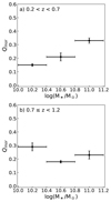 |
Fig. 6. Morphological quenching efficiency (Qmor) as a function of different stellar mass at 0.2 < z < 0.7 (panel a) and 0.7 ≤ z < 1.2 (panel b). The associated uncertainties are computed through error propagation, where the standard deviation of the sSFR in each stellar mass bin is taken to represent the error in the corresponding median sSFR. |
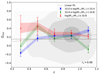 |
Fig. 7. Evolution of morphological quenching efficiency (Qmor) with the redshift interval Δz = 0.2. Different colors represent the trends in different stellar mass bins. The black dashed line displays the threshold of Qmor = 0.15. The extreme Qmor values within the upper and lower limits of 5% are excluded to reduce the impact of outliers on the error estimate. The correlation error is determined by resampling 1000 times using bootstrapping, where the error is defined as the standard deviation of the distribution of the median values over samples. The shaded areas represent 40% of the error bars. Based on a bootstrap sampling method, the distribution between Qmor and redshift is shown in the grey contours, with the best-fitting line shown in grey. Four iterations with outlier rejection based on a 3σ clipping criterion were applied to improve robustness. The small Spearman’s rank correlation coefficient (rs) indicates the weak relation between Qmor and redshift. |
Furthermore, in order to ascertain the impact of SFR on Qmor values, we employed a quantitative experiment following the same approach in Lu et al. (2021). Briefly, the simulation sample for each type of galaxies initially is composed of 10 000 galaxies with stellar mass uniformly distributed between 109.7 M⊙ and 1011.7 M⊙. We then hypothesize that the log(SFR) for both follow normal distributions, characterized by distinct means but a common variance of σ ∼ 0.7, obtained from fitting our real subsamples of ETDs and LTDs. Figure 8 presents a comparison between the simulated sample (left) and the actual observed sample (right). The top panels illustrate the distribution of sSFR for ETDs and LTDs, while the middle panels show the corresponding scatter sSFR-mass distributions. Subsequently, 500 galaxies were randomly selected from each class, and the corresponding median sSFR and Qmor were calculated. This process was repeated 1000 times and the resulting histogram of Qmor is presented at the bottom panels. Figure 8 reveals that when the mean SFRs of ETDs and LTDs differ by approximately ΔSFR = 0.3 M⊙ yr−1 in the simulated sample, we find that 73.6% of the Qmor is larger than 0.15, which is comparable with the real observed sample where the fraction of Qmor > 0.15 is 74.0%. As the variance σ ∼ 1.0 increases, the proportion decreases to 61.1%. Thus, the impact of morphological transitions in GV galaxies at 0.2 < z < 1.2 on star formation can be quantified by the threshold of Qmor ≥ 0.15, with a difference between the average SFR of ETDs and LTDs of ΔSFR = 0.3 M⊙ yr−1. These results slightly differ from the results in Lu et al. (2021), where Qmor > 0.2 with ΔSFR = 0.7 M⊙ yr−1 at 0.5 < z < 1.5. This bias may come from different redshift ranges and different morphological measurement methods based on images in different bands. For the latter, the morphological measurements in this work are based on high-resolution (PSF = 0.095″) HST/F814W images using a combination of UML and SML methods; namely, the two-step galaxy morphological classification framework (USmorph, see Song et al. 2024 for details). In addition, the morphologies for Lu et al. (2021) are based on measurements in low-resolution (PSF = 0.17″) HST/F160W images from the catalog of Huertas-Company et al. (2015), where the convolutional neural network (CNN, an SML method) is used to replicate human perception.
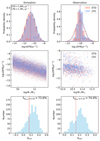 |
Fig. 8. Comparisons of simulation (left) and observations (right) results. In the left panels, we assumed that there are 10 000 galaxies with stellar mass spanning uniformly from 109.7 M⊙ to 1011.7 M⊙ in each simulation subsample (ETDs vs. LTDs). Both subsamples have normal distributions of SFR but the mean SFRs between them are different (see upper left corner for details). The upper left panel shows the normalized histograms of sSFR for ETDs (red) and LTDs (blue), fitted by using the normal distribution (dashed line). The corresponding mean sSFR values in the log scale are displayed near the vertical dashed lines. The center left panel presents the sSFR-mass distribution. The lower left panel depicts a histogram of Qmor, obtained by the random sampling of 500 galaxies in each simulation subsample, with the process repeated 1000 times. The red vertical dashed line represents the threshold of Qmor = 0.15, and the fraction of Qmor ≥ 0.15 is shown at the top. The right panels show similar results as the left panels, but for a real sample from this work, including 1296 ETDs and 1296 LTDs. |
3.4. Radial surface brightness
To further explore the difference in radial surface brightness between ETDs and LTDs, we focused on performing a two-dimensional Sérsic profile fitting on each galaxy in the I band image with GALFIT (Peng et al. 2010) to obtain the best-fit model and derive the structural parameters, including the center position, the effective radius re1, the Sérsic index, and the position angle. Then, we utilized the Photutils package in Python (Bradley et al. 2022) to drive the radial surface brightness of each galaxy, based on the original I band image and its best-fit model obtained. Finally, we averaged the resulting surface brightness profiles of all ETDs (or LTDs) to obtain a typical surface brightness profile for this type of galaxy. The point spread function (PSF) in the I band image was provided by Song et al. (2024).
In the top panels of Fig. 9, the solid and dashed red (blue) lines show the average surface brightness distribution of ETDs (LTDs) in the observations and the best-fit models at different redshift bins. The residuals can be derived from the difference between the original image and the best-fit model. The mean effective radii obtained by fitting galaxy images with GALFIT (Peng et al. 2010) are highlighted by the vertical dashed lines. Both the mean effective radius ⟨re⟩ and the mean Sérsic index ⟨n⟩ with associated ±1σ errors are marked on each panel. Compared to LTDs, we find that ETDs always have brighter surface brightness profiles, especially closer to the galaxy center or at < re. This is consistent with the larger values of ⟨n⟩ found in ETDs than LTDs, indicating that ETDs possess a more concentrated structure than LTDs. The Sérsic index distribution at the bottom of Fig. 9 can also approve this point that ETDs generally have larger Sérsic index distributions than LTDs and their medians ([n]) are larger as well, also shown as the vertical lines. At the bottom of each panel, the residuals of radial surface brightness between the original and modeled images are shown within 0.15, indicating the good performance of the model fitting. Typically, ETDs are more concentrated than LTDs in the regions with a radius of at least ≲0.3−0.4 arcsec. As cosmic time evolves, both ETDs and LTDs become more compact, probably due to gas consumption and accretion of the condensed components.
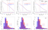 |
Fig. 9. Surface brightness profiles (top panels) of ETDs (red) and LTDs (blue) and Sérsic index distributions (bottom panels) in the I band. From left to right: Distributions at 0.2 < z < 0.7 (left) and 0.7 ≤ z < 1.2 (center), as well as the distribution over the entire redshift range (0.2 < z < 1.2, right), are shown. By fitting the surface brightness distribution of each galaxy using GALFIT (Peng et al. 2010) and then averaging the superposition, the effective radius re (also shown in vertical dashed lines) and the Sérsic index with ±1σ errors are imposed on each top panel. In each top panel, the average surface brightness profiles of the observed ETDs (LTDs) and their best-fit models are depicted by the solid and dashed red (blue) lines, respectively, whereas the residual between observation and model of ETDs (LTDs) is shown in red (blue). The point spread function (PSF) distribution is shown in grey. The bottom panels present the corresponding distribution of Sérsic index for each class of galaxies at a specific redshift bin. The median value of Sérsic index distribution for ETDs (LTDs) are marked and highlighted by the vertical dashed line in red (blue). The errors of median Sérsic indices represent the ±25th of median values. |
Regardless of evolution, we further explore the morphological dependence of ETDs and LTDs on the stellar mass. As shown in Fig. 10, the surface brightness and Séric index distribution are investigated again but in three different stellar mass bins. We can find that ETDs own smaller average ⟨re⟩ and larger average ⟨n⟩ and median [n] than LTDs in all three stellar mass ranges. For both ETDs and LTDs, more massive galaxies are more concentrated than less massive galaxies, because massive galaxies have larger average ⟨n⟩ and median [n]. Furthermore, we performed Kolmogorov–Smirnov (K-S) tests on the Sérsic index distributions shown in Figs. 9 and 10 to assess structural differences between ETDs and LTDs. The results show that in all three redshift bins and all three mass bins, the p-values are significantly smaller than 0.01, indicating that the Sérsic index distributions of ETDs and LTDs are significantly different in statistics. This suggests that stellar mass could have an impact on galaxy morphology to some extent, as massive galaxies might be able to constrain the assembly process by investigating their deep potential wells.
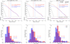 |
Fig. 10. Surface brightness profiles (top panels) and Sérsic index distributions (bottom panels) for ETDs (red) and LTDs (blue) in the I band. This figure is analogous to Fig. 9, but the panels from left to right present the results for M* bins of 10 ≤ log(M*/M⊙) < 10.4, 10.4 ≤ log(M*/M⊙)≤10.8, and log(M*/M⊙)≥10.8, respectively. |
To validate the robustness of our results, we also applied another method, iFIT (Breda et al. 2019), to quantify the radial surface brightness of the galaxy. The brief description of the iFIT software, the corresponding configuration, and supplementary results are provided in Appendix B. As shown in Fig. B.1 for the full sample, the average Sérsic index obtained by iFIT is n ∼ 1.3 for ETDs and n ∼ 1.0 for LTDs. Compared to GALFIT results, iFIT results also provide direct evidence that ETDs possess a more compact structure rather than an extended one. We also performed a K-S test on the Sérsic index measured by iFIT to verify the distribution differences between ETDs and LTDs. As expected, the p-values are smaller than 0.01 in both different redshift intervals and stellar mass bins, reconciling these results with the GALFIT results. It can be confirmed that ETDs and LTDs exhibit systematic differences in their structural properties. Notably, the consistent results of GALFIT and iFIT once again demonstrate the reliability of our results.
3.5. Environment
As an external mechanism, the environment can contribute to the reduction and cessation of star formation in galaxies. In the Local Universe, early-type passive galaxies are typically found in dense environments (e.g., galaxy groups and clusters), while late-type star-forming galaxies are predominantly located in less dense environments (Woo et al. 2013; Paspaliaris et al. 2023). However, the question of the effects the environment has on star formation at intermediate to high redshifts remains open. Observations reveal that the star formation of galaxies may either be enhanced in dense environments (Cooper et al. 2008; Koyama et al. 2013), showing no significant correlation with the environments (Randriamampandry et al. 2020; Cooke et al. 2023) or demonstrating a similar relationship to that observed in the Local Universe (Patel et al. 2009; Sobral et al. 2011). Since the MQ we have mainly focused on in this work is the internal mechanism affecting star formation in galaxies, the suppression of star formation may originate from internal or external mechanisms. To elucidate which mechanism is dominant in quenching galaxies, we analyzed the environmental differences between ETDs and LTDs using the environmental measurement, which was recently improved upon by Gu et al. (2020).
Rather than relying on traditional indicators of the local environment, which typically use the tenth nearest neighbor or the total count of nearby galaxies within a fixed radius (Dressler 1980), the environmental indicator can be refined by employing a Bayesian approach that incorporates the distances to all N neighboring galaxies (Ivezić et al. 2005). This method significantly improves the accuracy of density estimation (see Ivezić et al. 2005 for more details). To ensure a high level of precision in the redshift measurements for the COSMOS survey with HST/F814W detections, we initially constructed a magnitude-limited sample (Imag < 25) at 0.2 < z < 1.2. We then estimated the local surface density for each galaxy in the sample using the formula:
 (7)
(7)
where di denotes the projected distance to the i-th nearest neighbor within a redshift slice |Δz|< σz(1 + z) with σz = 0.04. Subsequently, we defined the dimensionless overdensity, 1 + δ′10, as the environment indicator:
 (8)
(8)
where  denotes the surface number density within a specific redshift slice. The denominator ⟨Σ′10⟩, a standard environmental tracer, can be calculated by multiplying the correction factor k′10 by the local surface density Σ′10, with the adopted value of k′10 being 0.06. The measurement of overdensity has been demonstrated to effectively trace low-redshift and high-redshift structures through the re-evaluation of several known galaxy groups and candidate clusters (Postman et al. 2012).
The top panels of Fig. 11 illustrate the overdensity distributions of ETDs (red) and LTDs (blue) in two redshift intervals. Both galaxy types exhibit comparable histograms and mean values for the environmental tracer. To further distinguish the differences in their respective environments, the cumulative distribution functions are provided in the bottom panels. Kolmogorov–Smirnov tests were conducted to compare ETDs and LTDs in two redshift intervals, determining whether both subsamples originate from the same underlying parent distribution. We adopted a limit of the K-S test probability, PKS(ETD, LTD)≤0.05 to show that the two samples exhibit significantly different environmental distributions at the 2σ level. Figure 11 shows that the high K-S test probabilities between ETDs and LTDs imply no significant environmental differences between the two subsamples in the GV population. Both ETDs and LTDs reside in similar environments, but the former have lower sSFR distribution (as shown in Fig. 5), which suggests that for massive (M* ≥ 1010 M⊙) GV galaxies at 0.2 < z < 1.2, environmental effects may not be the dominant factor affecting star formation in galaxies. Based on analyses from the FourStar Galaxy Evolution (ZFOURGE) survey, Kawinwanichakij et al. (2017) confirmed that environmental quenching is more effective for low-mass galaxies (M* < 1010 M⊙) at z ≲ 1.5, compared to their more massive counterparts (M* ≥ 1010 M⊙). This result aligns well with our findings.
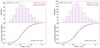 |
Fig. 11. Distributions (top panels) and cumulative probabilities (bottom panels) of overdensity at 0.2 < z < 0.7 (left) and 0.7 ≤ z < 1.2 (right), respectively. The red- and blue-shaded histograms represent ETDs and LTDs, respectively. The corresponding means and standard deviations are provided in the top-right corner of the top panel. The probabilities derived from the K-S tests for the two subsamples are indicated in the lower right corners of the bottom panels. |
4. Discussion
Previous studies have found that many physical properties of GV galaxies are characterized by distributions that are situated right between BC and RS galaxies. Such properties include the stellar mass, SFR, color, structure, and morphology (e.g., Gu et al. 2018; Ge et al. 2019; Sampaio et al. 2022), suggesting that GV galaxies are typically in the star-formation quenching phase (e.g., Martin et al. 2007; Nogueira-Cavalcante et al. 2018). This indicates that GV galaxies are an ideal laboratory for studying the effect of galaxy morphology on star formation quenching. Therefore, we selected a sample of 2592 massive (M* ≥ 1010 M⊙) GV galaxies at 0.2 < z < 1.2 and further separated them into two types: ETDs and LTDs. With an aim to explore the MQ mechanism, the physical properties of ETDs and LTDs have been analyzed in this work, including the nonparametric structure (i.e., Gini, C and M20), sSFR, radial surface brightness, and environment. Considering that star formation in galaxies typically involves both internal and external processes, such as the inner AGN feedback and the outer environment, we first tried to eliminate the influence of AGNs on their host galaxies (see Sect. 2.4.3), aiming to relieve the effect of AGN feedback on the galaxy morphology as well as on our results as much as possible. For the surrounding galaxy environment, as demonstrated in Sect. 3.5, a comparison of ETDs and LTDs reveals that the environments surrounding ETDs and LTDs are similar. However, our analysis reveals that ETDs exhibit lower sSFR compared to LTDs and are more morphologically concentrated, as indicated by their higher Gini and C, lower M20 values, and more compact radial surface brightness profiles. This suggests that the morphologies of massive (M* ≥ 1010 M⊙) GV galaxies are the primary factor affecting the star formation, compared to the environment, which can be reconciled with the results reported by Gu et al. (2021). These authors found that environmental quenching is more effective for low-mass galaxies at 0.5 < z < 1. It is worth noting that the comparison between ETDs and LTDs in this work was done after considering the mass-matching process, which means that both have similar distributions of stellar mass and redshift (see Sect. 2.4.3).
Moreover, to quantitatively describe the impact of quenching on star formation in galaxies, we used the morphological quenching efficiency parameter (Qmor) defined by Lu et al. (2021), which links the sSFR to the morphology of galaxies. Figures 6 and 7 illustrate that Qmor has no significant dependence on the redshift within the errors; however, more massive (M* > 1010.8 M⊙) galaxies seemingly have larger Qmor values than less massive galaxies, especially for low-mass galaxies with M* < 1010.4 M⊙ at z < 1. This would indicate that the MQ is related to stellar mass. More massive galaxies have stronger morphological effects on star formation. Based on our sample, we find that the values of Qmor are always greater than 0.15 within the margin of error. In the meantime, quantitative experiments on the impact of SFR on Qmor measurements (see Fig. 8) indicate that when we are assuming a uniform stellar mass distribution and a normal distribution of the SFR for each type of galaxies, the proportion of Qmor ≥ 0.15 can be close to ∼75% when the difference between the mean SFRs of ETDs and LTDs is approximately 0.3 M⊙ yr−1. This may indicate that the discrepancy between the mean SFRs of ETDs and LTDs in our GV sample is not significantly huge (only ∼0.3 M⊙ yr−1) and the degree of the MQ in our GV galaxies is quantified by this value (Qmor = 0.15).
To reveal the detailed discrepancy of radial surface brightness profiles between ETDs and LTDs, we adopted a Sérsic model to fit the morphology of each galaxy and compared the average radial profile of ETDs with that of LTDs. The top panels of Fig. 9 show that as the radius approaches the center, the average profile of ETDs is brighter than that of LTDs, suggesting that ETDs statistically have more compact centers than LTDs, which agrees with the distributions of Sérsic indices as shown in the bottom panels of Fig. 9. As cosmic time evolves, all galaxies become more concentrated, probably due to the mass assembly. As shown in Fig. 10, we also find that more massive (M* > 1010.8 M⊙) galaxies including ETDs and LTDs with higher Sérsic indices (average ⟨n⟩∼1.7 and median [n]∼1.5) are more bulge-dominated than less massive (M* < 1010.4 M⊙) galaxies with lower Sérsic indices (average ⟨n⟩∼1.3 and median [n]∼1.2). This is consistent with what we find in the Qmor evolution of Fig. 7, providing observed evidence that the stellar mass plays a critical role in MQ. In addition, we adopted an alternative fitting tool (i.e., iFIT, see Appendix B for details) to perform an independent structural analysis. As shown in Fig. B.1c, the results indicate that the average Sérsic index of ETDs is approximately n ∼ 1.3, while that of LTDs is around n ∼ 1.0 across the entire sample. This trend further reinforces the observation that ETDs possess more centrally concentrated, bulge-dominated structures than LTDs. The cross-validation between the two tools demonstrates the robustness of our results and supports the systematic structural differences between ETDs and LTDs from multiple perspectives. The MQ is mainly dominated by massive bulges.
Previous studies have provided some consistent clues about the MQ from observations. Whitaker et al. (2015) investigated how the galaxy structure affects the relationship between SFR and stellar mass. They highlighted the rapid increase of bulges in massive galaxies at z ∼ 2 and proposed that prominent bulges may be a crucial factor in the quenching process. Additionally, Franx et al. (2008) demonstrated that surface density and inferred velocity dispersion of galaxies correlate more strongly with sSFR and color than with stellar mass, suggesting that central density and dynamical properties have a greater influence on star formation history. Specifically, galaxies with prominent bulges typically exhibit lower sSFRs and redder colors compared to disk-like galaxies. This observation supports the role of MQ mechanisms in regulating star formation activity within galaxies and underscores the crucial role of galaxy structure in their evolutionary processes.
5. Summary
In this work, we analyzed the MQ impact on star formation of massive (M* ≥ 1010 M⊙) GV galaxies in the COSMOS field at 0.2 < z < 1.2, by making a comparison between ETDs and LTDs from different physical properties, including the nonparametric structure (i.e., Gini vs. C, M20), sSFR, the radial surface brightness profile, and their environments. Our main results are presented below.
-
After the removal of as many AGN candidates as possible, we find that ETDs show higher Gini and C, more negative M20, and lower sSFRs than LTDs. This suggests that ETDs have more concentrated morphologies and experience more rapid quenching of star formation, compared to LTDs. In addition, the average radial surface brightness of ETDs is brighter and more compact than that of LTDs, especially near the center. More massive galaxies are concentrated than less massive ones. All galaxies become more and more bulge-dominated over cosmic time.
-
Considering the influence of the external environment on the star formation of galaxies, we measured the environment following an improved approach mentioned in Gu et al. (2020) and found that there is no significant difference in environment between ETDs and LTDs. This suggests that the environment may not be a dominant factor in the quenching of star formation for massive (M* ≥ 1010 M⊙) GV galaxies at 0.2 < z < 1.2.
-
Excluding the influence of external environments, we have sought to quantify the impact of morphological quenching efficiency on star formation by the dimensionless parameter Qmor, following the definition of Lu et al. (2021). Our findings indicate that the fraction of Qmor > 0.15 approaches ∼75% when the difference of the mean SFR between ETDs and LTDs is approximately 0.3 M⊙ yr−1. Overall, Qmor tends to be more associated with the stellar mass than redshift, especially for massive (M* > 1010.8 M⊙) galaxies, indicating that more massive galaxies could experience stronger morphological quenching process than less massive galaxies at z < 1.
All in all, we find that ETDs have weaker star formation activities but more compact morphological structures than LTDs. After excluding the internal (e.g., AGNs and stellar masses) and external (e.g., environments) effects, we propose that the morphology plays an important role in quenching the star formation of galaxies, particularly in the high-mass (M* > 1010.8 M⊙) end.
It is defined as the half-light radius in the I band image.
Acknowledgments
This work is supported by the China Manned Space Project (No. CMS-CSST-2021-A07). The numerical calculations in this paper have been done on the computing facilities in the High Performance Computing Platform of Anqing Normal University. S.L. acknowledges the support from the Key Laboratory of Modern Astronomy and Astrophysics (Nanjing University) by the Ministry of Education. Z.S.L. acknowledges the support from Hong Kong Innovation and Technology Fund through the Research Talent Hub program (PiH/022/22GS).
References
- Abraham, R. G., van den Bergh, S., & Nair, P. 2003, ApJ, 588, 218 [NASA ADS] [CrossRef] [Google Scholar]
- Angthopo, J., Ferreras, I., & Silk, J. 2020, MNRAS, 495, 2720 [NASA ADS] [CrossRef] [Google Scholar]
- Bait, O., Barway, S., & Wadadekar, Y. 2017, MNRAS, 471, 2687 [NASA ADS] [CrossRef] [Google Scholar]
- Baldry, I. K., Balogh, M. L., Bower, R., Glazebrook, K., & Nichol, R. C. 2004, AIP Conf. Ser., 743, 106 [Google Scholar]
- Bates, D. J., Tojeiro, R., Newman, J. A., et al. 2019, MNRAS, 486, 3059 [CrossRef] [Google Scholar]
- Bell, E. F., Papovich, C., Wolf, C., et al. 2005, ApJ, 625, 23 [Google Scholar]
- Bershady, M. A., Jangren, A., & Conselice, C. J. 2000, AJ, 119, 2645 [NASA ADS] [CrossRef] [Google Scholar]
- Bluck, A. F. L., Mendel, J. T., Ellison, S. L., et al. 2014, MNRAS, 441, 599 [NASA ADS] [CrossRef] [Google Scholar]
- Bournaud, F., & Elmegreen, B. G. 2009, ApJ, 694, L158 [CrossRef] [Google Scholar]
- Bradley, L., Sipőcz, B., Robitaille, T., et al. 2022, https://doi.org/10.5281/zenodo.7419741 [Google Scholar]
- Brammer, G. B., van Dokkum, P. G., & Coppi, P. 2008, ApJ, 686, 1503 [Google Scholar]
- Brammer, G. B., Whitaker, K. E., van Dokkum, P. G., et al. 2009, ApJ, 706, L173 [Google Scholar]
- Breda, I., Papaderos, P., Gomes, J. M., & Amarantidis, S. 2019, A&A, 632, A128 [NASA ADS] [CrossRef] [EDP Sciences] [Google Scholar]
- Bruzual, G., & Charlot, S. 2003, MNRAS, 344, 1000 [NASA ADS] [CrossRef] [Google Scholar]
- Bundy, K., Scarlata, C., Carollo, C. M., et al. 2010, ApJ, 719, 1969 [NASA ADS] [CrossRef] [Google Scholar]
- Calzetti, D., Armus, L., Bohlin, R. C., et al. 2000, ApJ, 533, 682 [NASA ADS] [CrossRef] [Google Scholar]
- Camps-Fariña, A., Mérida, R. M., Sánchez-Blázquez, P., & Sánchez, S. F. 2024, A&A, 691, A56 [NASA ADS] [CrossRef] [EDP Sciences] [Google Scholar]
- Cano-Díaz, M., Ávila-Reese, V., Sánchez, S. F., et al. 2019, MNRAS, 488, 3929 [Google Scholar]
- Chabrier, G. 2003, PASP, 115, 763 [Google Scholar]
- Chang, W., Fang, G., Gu, Y., et al. 2022, ApJ, 936, 47 [Google Scholar]
- Conselice, C. J. 2003, ApJS, 147, 1 [NASA ADS] [CrossRef] [Google Scholar]
- Cook, R. H. W., Cortese, L., Catinella, B., & Robotham, A. 2020, MNRAS, 493, 5596 [NASA ADS] [CrossRef] [Google Scholar]
- Cooke, K. C., Kartaltepe, J. S., Rose, C., et al. 2023, ApJ, 942, 49 [NASA ADS] [CrossRef] [Google Scholar]
- Cooper, M. C., Newman, J. A., Weiner, B. J., et al. 2008, MNRAS, 383, 1058 [Google Scholar]
- Corcho-Caballero, P., Casado, J., Ascasibar, Y., & García-Benito, R. 2021, MNRAS, 507, 5477 [NASA ADS] [CrossRef] [Google Scholar]
- Cortese, L., Catinella, B., & Smith, R. 2021, PASA, 38, e035 [NASA ADS] [CrossRef] [Google Scholar]
- Cowie, L. L., Songaila, A., Hu, E. M., & Cohen, J. G. 1996, AJ, 112, 839 [Google Scholar]
- Crocker, A. F., Bureau, M., Young, L. M., & Combes, F. 2011, MNRAS, 410, 1197 [NASA ADS] [CrossRef] [Google Scholar]
- Dimauro, P., Daddi, E., Shankar, F., et al. 2022, MNRAS, 513, 256 [NASA ADS] [CrossRef] [Google Scholar]
- Donley, J. L., Koekemoer, A. M., Brusa, M., et al. 2012, ApJ, 748, 142 [Google Scholar]
- Dressler, A. 1980, ApJ, 236, 351 [Google Scholar]
- Estrada-Carpenter, V., Papovich, C., Momcheva, I., et al. 2023, ApJ, 951, 115 [Google Scholar]
- Fang, J. J., Faber, S. M., Salim, S., Graves, G. J., & Rich, R. M. 2012, ApJ, 761, 23 [NASA ADS] [CrossRef] [Google Scholar]
- Fang, J. J., Faber, S. M., Koo, D. C., & Dekel, A. 2013, ApJ, 776, 63 [NASA ADS] [CrossRef] [Google Scholar]
- Franx, M., van Dokkum, P. G., Förster Schreiber, N. M., et al. 2008, ApJ, 688, 770 [NASA ADS] [CrossRef] [Google Scholar]
- Ge, X., Gu, Q.-S., Chen, Y.-Y., & Ding, N. 2019, RAA, 19, 027 [Google Scholar]
- Gensior, J., Kruijssen, J. M. D., & Keller, B. W. 2020, MNRAS, 495, 199 [NASA ADS] [CrossRef] [Google Scholar]
- Gu, Y., Fang, G., Yuan, Q., Cai, Z., & Wang, T. 2018, ApJ, 855, 10 [Google Scholar]
- Gu, Y., Fang, G., Yuan, Q., et al. 2019, ApJ, 884, 172 [NASA ADS] [CrossRef] [Google Scholar]
- Gu, Y., Fang, G., Yuan, Q., & Lu, S. 2020, PASP, 132, 054101 [CrossRef] [Google Scholar]
- Gu, Y., Fang, G., Yuan, Q., Lu, S., & Liu, S. 2021, ApJ, 921, 60 [NASA ADS] [CrossRef] [Google Scholar]
- Guglielmo, V., Poggianti, B. M., Moretti, A., et al. 2015, MNRAS, 450, 2749 [NASA ADS] [CrossRef] [Google Scholar]
- Hasinger, G., Capak, P., Salvato, M., et al. 2018, ApJ, 858, 77 [Google Scholar]
- Huertas-Company, M., Gravet, R., Cabrera-Vives, G., et al. 2015, ApJS, 221, 8 [NASA ADS] [CrossRef] [Google Scholar]
- Ilbert, O., Arnouts, S., McCracken, H. J., et al. 2006, A&A, 457, 841 [NASA ADS] [CrossRef] [EDP Sciences] [Google Scholar]
- Ilbert, O., Capak, P., Salvato, M., et al. 2009, ApJ, 690, 1236 [NASA ADS] [CrossRef] [Google Scholar]
- Ivezić, Ž., Vivas, A. K., Lupton, R. H., & Zinn, R. 2005, AJ, 129, 1096 [Google Scholar]
- Jian, H.-Y., Lin, L., Oguri, M., et al. 2018, PASJ, 70, S23 [CrossRef] [Google Scholar]
- Kawinwanichakij, L., Papovich, C., Quadri, R. F., et al. 2017, ApJ, 847, 134 [NASA ADS] [CrossRef] [Google Scholar]
- Koyama, Y., Smail, I., Kurk, J., et al. 2013, MNRAS, 434, 423 [CrossRef] [Google Scholar]
- Koyama, S., Koyama, Y., Yamashita, T., et al. 2019, ApJ, 874, 142 [NASA ADS] [CrossRef] [Google Scholar]
- Laigle, C., McCracken, H. J., Ilbert, O., et al. 2016, ApJS, 224, 24 [Google Scholar]
- Lee, J. H., Park, C., Hwang, H. S., & Kwon, M. 2024, ApJ, 966, 113 [NASA ADS] [CrossRef] [Google Scholar]
- Liu, C., Hao, L., Wang, H., & Yang, X. 2019, ApJ, 878, 69 [NASA ADS] [CrossRef] [Google Scholar]
- Lotz, J. M., Primack, J., & Madau, P. 2004, AJ, 128, 163 [NASA ADS] [CrossRef] [Google Scholar]
- Lu, S., Fang, G., Gu, Y., et al. 2021, ApJ, 913, 81 [CrossRef] [Google Scholar]
- Madau, P., & Dickinson, M. 2014, ARA&A, 52, 415 [Google Scholar]
- Martig, M., Bournaud, F., Teyssier, R., & Dekel, A. 2009, ApJ, 707, 250 [Google Scholar]
- Martin, D. C., Wyder, T. K., Schiminovich, D., et al. 2007, ApJS, 173, 342 [NASA ADS] [CrossRef] [Google Scholar]
- Muzzin, A., Marchesini, D., Stefanon, M., et al. 2013, ApJS, 206, 8 [Google Scholar]
- Nogueira-Cavalcante, J. P., Gonçalves, T. S., Menéndez-Delmestre, K., & Sheth, K. 2018, MNRAS, 473, 1346 [Google Scholar]
- Pandya, V., Brennan, R., Somerville, R. S., et al. 2017, MNRAS, 472, 2054 [NASA ADS] [CrossRef] [Google Scholar]
- Paspaliaris, E. D., Xilouris, E. M., Nersesian, A., et al. 2023, A&A, 669, A11 [NASA ADS] [CrossRef] [EDP Sciences] [Google Scholar]
- Patel, S. G., Holden, B. P., Kelson, D. D., Illingworth, G. D., & Franx, M. 2009, ApJ, 705, L67 [Google Scholar]
- Peng, C. Y., Ho, L. C., Impey, C. D., & Rix, H.-W. 2010, AJ, 139, 2097 [Google Scholar]
- Postman, M., Lauer, T. R., Donahue, M., et al. 2012, ApJ, 756, 159 [Google Scholar]
- Pozzetti, L., Bolzonella, M., Zucca, E., et al. 2010, A&A, 523, A13 [NASA ADS] [CrossRef] [EDP Sciences] [Google Scholar]
- Prevot, M. L., Lequeux, J., Maurice, E., Prevot, L., & Rocca-Volmerange, B. 1984, A&A, 132, 389 [Google Scholar]
- Randriamampandry, S. M., Vaccari, M., & Hess, K. M. 2020, MNRAS, 499, 948 [NASA ADS] [CrossRef] [Google Scholar]
- Rasmussen, J., Ponman, T. J., & Mulchaey, J. S. 2006, MNRAS, 370, 453 [NASA ADS] [CrossRef] [Google Scholar]
- Rodriguez-Gomez, V., Snyder, G. F., Lotz, J. M., et al. 2019, MNRAS, 483, 4140 [NASA ADS] [CrossRef] [Google Scholar]
- Ruffa, I., & Davis, T. A. 2024, Galaxies, 12, 36 [Google Scholar]
- Sajina, A., Lacy, M., & Pope, A. 2022, Universe, 8, 356 [NASA ADS] [CrossRef] [Google Scholar]
- Salim, S. 2014, Serb. Astron. J., 189, 1 [NASA ADS] [CrossRef] [Google Scholar]
- Salim, S., Fang, J. J., Rich, R. M., Faber, S. M., & Thilker, D. A. 2012, ApJ, 755, 105 [NASA ADS] [CrossRef] [Google Scholar]
- Sampaio, V. M., de Carvalho, R. R., Ferreras, I., Aragón-Salamanca, A., & Parker, L. C. 2022, MNRAS, 509, 567 [Google Scholar]
- Sampaio, V. M., Aragón-Salamanca, A., Merrifield, M. R., et al. 2023, MNRAS, 524, 5327 [Google Scholar]
- Satyapal, S., Secrest, N. J., Ricci, C., et al. 2017, ApJ, 848, 126 [Google Scholar]
- Schawinski, K., Kaviraj, S., Khochfar, S., et al. 2007, ApJS, 173, 512 [NASA ADS] [CrossRef] [Google Scholar]
- Schawinski, K., Urry, C. M., Simmons, B. D., et al. 2014, MNRAS, 440, 889 [Google Scholar]
- Scoville, N., Aussel, H., Brusa, M., et al. 2007, ApJS, 172, 1 [Google Scholar]
- Smith, D., Haberzettl, L., Porter, L. E., et al. 2022, MNRAS, 517, 4575 [Google Scholar]
- Sobral, D., Best, P. N., Smail, I., et al. 2011, MNRAS, 411, 675 [NASA ADS] [CrossRef] [Google Scholar]
- Song, J., Fang, G., Ba, S., et al. 2024, ApJS, 272, 42 [NASA ADS] [CrossRef] [Google Scholar]
- Su, Y., Irwin, J. A., White, R. E., III, & Cooper, M. C. 2015, ApJ, 806, 156 [NASA ADS] [CrossRef] [Google Scholar]
- Su, K.-Y., Hopkins, P. F., Hayward, C. C., et al. 2019, MNRAS, 487, 4393 [NASA ADS] [CrossRef] [Google Scholar]
- Thilker, D. A., Bianchi, L., Schiminovich, D., et al. 2010, ApJ, 714, L171 [NASA ADS] [CrossRef] [Google Scholar]
- Treyer, M., Schiminovich, D., Johnson, B. D., et al. 2010, ApJ, 719, 1191 [NASA ADS] [CrossRef] [Google Scholar]
- Wang, L., Norberg, P., Gunawardhana, M. L. P., et al. 2016, MNRAS, 461, 1898 [Google Scholar]
- Wang, T., Elbaz, D., Alexander, D. M., et al. 2017, A&A, 601, A63 [NASA ADS] [CrossRef] [EDP Sciences] [Google Scholar]
- Weaver, J. R., Kauffmann, O. B., Ilbert, O., et al. 2022, ApJS, 258, 11 [NASA ADS] [CrossRef] [Google Scholar]
- Whitaker, K. E., Franx, M., Bezanson, R., et al. 2015, ApJ, 811, L12 [NASA ADS] [CrossRef] [Google Scholar]
- Woo, J., Dekel, A., Faber, S. M., et al. 2013, MNRAS, 428, 3306 [CrossRef] [Google Scholar]
- Wright, R. J., Lagos, C. D. P., Power, C., et al. 2022, MNRAS, 516, 2891 [NASA ADS] [CrossRef] [Google Scholar]
- Wuyts, S., Förster Schreiber, N. M., Lutz, D., et al. 2011, ApJ, 738, 106 [Google Scholar]
- Wyder, T. K., Martin, D. C., Schiminovich, D., et al. 2007, ApJS, 173, 293 [Google Scholar]
- Yesuf, H. M., Ho, L. C., & Faber, S. M. 2021, ApJ, 923, 205 [NASA ADS] [CrossRef] [Google Scholar]
Appendix A: I band image: ETDs and LTDs
Figure A.1 presents images of ETDs and LTDs at 0.7 ≤ z < 1.2 in bins of Δz = 0.1, including the galaxy ID from the COSMOS2020 catalog, photometric redshift, and morphological parameters (Gini, M20, and concentration C) derived from the catalog by Song et al. (2024).
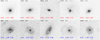 |
Fig. A.1. I band images of ETDs (red) and LTDs (blue), analogous to those presented in Fig. 4, with panels from left to right showing galaxies at 0.7 ≤ z < 1.2. |
Appendix B: iFIT
Apart from GALFIT, the second method, iFIT, was adopted to quantify the radial surface brightness of the galaxy in this work. This is a tool specifically designed by Breda et al. (2019). The strength of iFIT lies in its fitting methodology based on the Sérsic law, which determines an equivalent Sérsic model by searching for the best match between observed light growth curves and the variation of surface brightness with radius. This approach differs from traditional methods that rely on χ2 minimization for fitting individual data points. The configuration of iFIT (Breda et al. 2019) is significantly less sensitive to PSF convolution effects and surface brightness constraints compared to conventional methods. In addition, iFIT (Breda et al. 2019) is robust enough to accommodate imperfect Sérsic profiles, eliminating the need for initial parameter estimates and facilitating rapid convergence to a unique solution. This makes iFIT particularly well-suited for the automated structural characterization of irregular galaxies. The public availability of iFIT provides an efficient tool for the characterization of large galaxy samples.
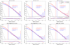 |
Fig. B.1. Average surface brightness profiles of ETDs (red) and LTDs (blue) in the I band at different redshift intervals (top panels) and stellar mass bins (bottom panels). By fitting the surface brightness distribution of galaxies using iFIT (Breda et al. 2019), the best-fit model profiles are shown in solid lines. The corresponding effective radius, re, (also shown as a vertical dashed line) and the Sérsic index, n, with absolute deviations are obtained and printed at the top right of each panel. The residual between the average surface brightness profiles of observed ETDs (LTDs) and their best-fit model profiles is displayed at the bottom. The PSF distribution is displayed in gray. |
To compare the radial surface brightness differences between ETDs and LTDs in the I band, we first extracted the radial surface profile of each galaxy with a step of Δre = 2 pixels, beyond > 2re, aiming to capture the faint outer edges of each galaxy as accurately as possible. Then, we adopted this radial surface brightness as input, considering the PSF convolution to obtain the best-fitting Sérsic model by using iFIT (Breda et al. 2019). We also repeat the iFIT measurements on the average radial surface brightness within different redshift intervals and stellar mass bins. In Fig. B.1, the points with error bars and solid lines represent the average surface brightness distribution of the observed ETDs (red) and LTDs (blue), along with the best-fit models obtained from iFIT. The residuals are derived from the difference between the interpolated observed data and the best-fit model. The corresponding best-fitted effective radii (also shown in vertical dashed lines) and Sérsic indices are shown on each panel, consistent with the results considering the statistical mean and median for each galaxy using iFIT. Compared to LTDs, it can be found that ETDs consistently have brighter surface brightness profiles, especially near the galaxy center or at < re, at least within the 0.3-0.4 arcsec range. This indicates that ETDs have a more concentrated structure with a more pronounced bulge, while LTDs likely have a more extended structure, which is consistent with GALFIT results shown in the main context.
Additionally, we notice that the structural parameters derived from iFIT (Breda et al. 2019) are systematically smaller than those obtained from GALFIT (Peng et al. 2010). The average differences are Δn ≈ 0.5 and Δre ≈ 0.1 arcsec, respectively. This discrepancy may first arise from methodological measurements between the two tools. For iFIT, it is necessary to extract one-dimensional radial surface brightness profiles from the images before fitting, whereas GALFIT allows for direct two-dimensional modeling of the images. And the difference may also be attributed to the image resolution of our sample. Due to the limited resolution of the galaxy images, the sampling data points of the reliable radial surface brightness available for analysis are reduced. The undersampling rate along the radius may be exacerbated by high-redshift GV galaxies with smaller morphologies, compared to local or high-redshift star-forming galaxies. Although we have made efforts to trace the faint outer regions (> 2re) in the I band images, the sparse radial sampling still limits our ability to fully recover the extended light profiles. As shown in Fig. B.1, the uncertainty in the extracted surface brightness values clearly increases with the radius. High-resolution images for high-redshift galaxies achieved in the future could help improve the structural measurements.
All Figures
|
Fig. 1. Distribution of stellar mass as a function of redshift. The boundaries of mass completeness in different fixed redshift bins (Δz = 0.25) are shown in green. The solid black line represents the best fitting of boundaries by the parameterized function Mmin(z) = 1.28ln(z)+9.78. The mass threshold (M* = 1010 M⊙) adopted in this work is present in the dashed back line, which could ensure a ≥95% completeness up to z ∼ 1.2. The background gray dots represent the parent sample selected from the COSMOS2020 catalog (see Sect. 2.1). |
| In the text | |
|
Fig. 2. Relationships between the extinction-corrected rest-frame U − V and stellar mass at 0.2 < z < 0.7 (left) and 0.7 ≤ z < 1.2 (right). The gray contours and mosaics in the background indicate the relative density in the color-mass panel. The criteria from Wang et al. (2017) was adopted to separate galaxies into RS, GV, and BC, respectively, as shown in orange lines in each panel. Based on the morphological classification from Song et al. (2024), the GV galaxies were further divided into two types, including early-type disk (ETD: red) and late-type disk (LTD: blue), separately. Both subsamples excluded the contamination from AGN candidates and considered the mass matching (see Sects. 2.4.2 and 2.4.3 for details). |
| In the text | |
|
Fig. 3. Distributions of ETDs (red) and LTDs (blue) in the Gini-M20 (top panels) and Gini-C (bottom panels) spaces within three stellar mass bins (left: 10.0 ≤ log(M*/M⊙) < 10.4, middle: 10.4 ≤ log(M*/M⊙) < 10.8, right: log(M*/M⊙)≥10.8). The red (blue) background represents the number density distribution of ETDs (LTDs) in each space. The red (blue) contours enclose 30%, 50%, and 70% of the respective subsamples. The red (blue) diamond indicates the median value of ETDs (LTDs) in each space, with ±25th percentile uncertainties. The corresponding median values and uncertainties are displayed at the bottom of each panel. |
| In the text | |
|
Fig. 4. Example images of ETDs (the first row) and LTDs (the second row) at 0.2 < z < 0.7 in the I band (see Fig. A.1 for example images at 0.7 ≤ z < 1.2). The corresponding information of each ETD (LTD) galaxy is depicted in red (blue) on the image, including the galaxy ID from the COSMOS2020 catalog, photometric redshift, Gini coefficient, M20 index, and the concentration, C. |
| In the text | |
|
Fig. 5. Relation between sSFR and stellar mass for ETDs (red) and LTD (blue). Within each redshift bin, both ETDs and LTDs are separated into three stellar mass ranges: 10.0 ≤ log(M*/M⊙) < 10.4, 10.4 ≤ log(M*/M⊙) < 10.8, and log(M*/M⊙)≥10.8. The median values of the distributions for ETDs and LTDs are shown in red and blue squares, respectively. The corresponding standard error of the median is derived from 1000 bootstrap estimates for the sample in a given stellar mass bin. |
| In the text | |
|
Fig. 6. Morphological quenching efficiency (Qmor) as a function of different stellar mass at 0.2 < z < 0.7 (panel a) and 0.7 ≤ z < 1.2 (panel b). The associated uncertainties are computed through error propagation, where the standard deviation of the sSFR in each stellar mass bin is taken to represent the error in the corresponding median sSFR. |
| In the text | |
|
Fig. 7. Evolution of morphological quenching efficiency (Qmor) with the redshift interval Δz = 0.2. Different colors represent the trends in different stellar mass bins. The black dashed line displays the threshold of Qmor = 0.15. The extreme Qmor values within the upper and lower limits of 5% are excluded to reduce the impact of outliers on the error estimate. The correlation error is determined by resampling 1000 times using bootstrapping, where the error is defined as the standard deviation of the distribution of the median values over samples. The shaded areas represent 40% of the error bars. Based on a bootstrap sampling method, the distribution between Qmor and redshift is shown in the grey contours, with the best-fitting line shown in grey. Four iterations with outlier rejection based on a 3σ clipping criterion were applied to improve robustness. The small Spearman’s rank correlation coefficient (rs) indicates the weak relation between Qmor and redshift. |
| In the text | |
|
Fig. 8. Comparisons of simulation (left) and observations (right) results. In the left panels, we assumed that there are 10 000 galaxies with stellar mass spanning uniformly from 109.7 M⊙ to 1011.7 M⊙ in each simulation subsample (ETDs vs. LTDs). Both subsamples have normal distributions of SFR but the mean SFRs between them are different (see upper left corner for details). The upper left panel shows the normalized histograms of sSFR for ETDs (red) and LTDs (blue), fitted by using the normal distribution (dashed line). The corresponding mean sSFR values in the log scale are displayed near the vertical dashed lines. The center left panel presents the sSFR-mass distribution. The lower left panel depicts a histogram of Qmor, obtained by the random sampling of 500 galaxies in each simulation subsample, with the process repeated 1000 times. The red vertical dashed line represents the threshold of Qmor = 0.15, and the fraction of Qmor ≥ 0.15 is shown at the top. The right panels show similar results as the left panels, but for a real sample from this work, including 1296 ETDs and 1296 LTDs. |
| In the text | |
|
Fig. 9. Surface brightness profiles (top panels) of ETDs (red) and LTDs (blue) and Sérsic index distributions (bottom panels) in the I band. From left to right: Distributions at 0.2 < z < 0.7 (left) and 0.7 ≤ z < 1.2 (center), as well as the distribution over the entire redshift range (0.2 < z < 1.2, right), are shown. By fitting the surface brightness distribution of each galaxy using GALFIT (Peng et al. 2010) and then averaging the superposition, the effective radius re (also shown in vertical dashed lines) and the Sérsic index with ±1σ errors are imposed on each top panel. In each top panel, the average surface brightness profiles of the observed ETDs (LTDs) and their best-fit models are depicted by the solid and dashed red (blue) lines, respectively, whereas the residual between observation and model of ETDs (LTDs) is shown in red (blue). The point spread function (PSF) distribution is shown in grey. The bottom panels present the corresponding distribution of Sérsic index for each class of galaxies at a specific redshift bin. The median value of Sérsic index distribution for ETDs (LTDs) are marked and highlighted by the vertical dashed line in red (blue). The errors of median Sérsic indices represent the ±25th of median values. |
| In the text | |
|
Fig. 10. Surface brightness profiles (top panels) and Sérsic index distributions (bottom panels) for ETDs (red) and LTDs (blue) in the I band. This figure is analogous to Fig. 9, but the panels from left to right present the results for M* bins of 10 ≤ log(M*/M⊙) < 10.4, 10.4 ≤ log(M*/M⊙)≤10.8, and log(M*/M⊙)≥10.8, respectively. |
| In the text | |
|
Fig. 11. Distributions (top panels) and cumulative probabilities (bottom panels) of overdensity at 0.2 < z < 0.7 (left) and 0.7 ≤ z < 1.2 (right), respectively. The red- and blue-shaded histograms represent ETDs and LTDs, respectively. The corresponding means and standard deviations are provided in the top-right corner of the top panel. The probabilities derived from the K-S tests for the two subsamples are indicated in the lower right corners of the bottom panels. |
| In the text | |
|
Fig. A.1. I band images of ETDs (red) and LTDs (blue), analogous to those presented in Fig. 4, with panels from left to right showing galaxies at 0.7 ≤ z < 1.2. |
| In the text | |
|
Fig. B.1. Average surface brightness profiles of ETDs (red) and LTDs (blue) in the I band at different redshift intervals (top panels) and stellar mass bins (bottom panels). By fitting the surface brightness distribution of galaxies using iFIT (Breda et al. 2019), the best-fit model profiles are shown in solid lines. The corresponding effective radius, re, (also shown as a vertical dashed line) and the Sérsic index, n, with absolute deviations are obtained and printed at the top right of each panel. The residual between the average surface brightness profiles of observed ETDs (LTDs) and their best-fit model profiles is displayed at the bottom. The PSF distribution is displayed in gray. |
| In the text | |
Current usage metrics show cumulative count of Article Views (full-text article views including HTML views, PDF and ePub downloads, according to the available data) and Abstracts Views on Vision4Press platform.
Data correspond to usage on the plateform after 2015. The current usage metrics is available 48-96 hours after online publication and is updated daily on week days.
Initial download of the metrics may take a while.