| Issue |
A&A
Volume 699, July 2025
|
|
|---|---|---|
| Article Number | A327 | |
| Number of page(s) | 20 | |
| Section | Cosmology (including clusters of galaxies) | |
| DOI | https://doi.org/10.1051/0004-6361/202452410 | |
| Published online | 23 July 2025 | |
Simulation-based inference benchmark for weak lensing cosmology
1
Université Paris Cité, CNRS, Astroparticule et Cosmologie, F-75013 Paris, France
2
Université Paris Cité, Université Paris-Saclay, CEA, CNRS, AIM, F-91191 Gif-sur-Yvette, France
3
Université Paris-Saclay, Université Paris Cité, CEA, CNRS, AIM, 91191 Gif-sur-Yvette, France
4
University of Liège, Liège, Belgium
5
Université Paris Cité, CNRS, CEA, Astroparticule et Cosmologie, F-75013 Paris, France
6
Sony Computer Science Laboratories – Rome, Joint Initiative CREF-SONY, Centro Ricerche Enrico Fermi, Via Panisperna 89/A, 00184 Rome, Italy
7
Center for Computational Astrophysics, Flatiron Institute, 162 5th Ave, New York, NY 10010, USA
8
Department of Astrophysical Sciences, Princeton University, Peyton Hall, 4 Ivy Lane, Princeton, NJ 08544, USA
9
Department of Physics, Université de Montréal, Montréal H2V 0B3, Canada
10
Mila – Quebec Artificial Intelligence Institute, Montréal H2S 3H1, Canada
11
Ciela – Montreal Institute for Astrophysical Data Analysis and Machine Learning, Montréal H2V 0B3, Canada
⋆ Corresponding author.
Received:
29
September
2024
Accepted:
20
March
2025
Abstract
Context. Standard cosmological analysis, which is based on two-point statistics, fails to extract all the information embedded in the cosmological data. This limits our ability to precisely constrain cosmological parameters. Through willingness to use modern analysis techniques to match the power of upcoming telescopes, recent years have seen a paradigm shift from analytical likelihood-based to simulation-based inference. However, such methods require a large number of costly simulations.
Aims. We focused on full-field inference, which is considered the optimal form of inference as it enables the recovery of cosmological constraints from simulations without any loss of cosmological information. Our objective is to review and benchmark several ways of conducting full-field inference to gain insight into the number of simulations required for each method. Specifically, we made a distinction between explicit inference methods that require an explicit form of the likelihood, such that it can be evaluated and thus sampled through sampling schemes and implicit inference methods that can be used when only an implicit version of the likelihood is available through simulations. Moreover, it is crucial for explicit full-field inference to use a differentiable forward model. Similarly, we aim to discuss the advantages of having differentiable forward models for implicit full-field inference.
Methods. We used the sbi_lens package (https://github.com/DifferentiableUniverseInitiative/sbi_lens), which provides a fast and differentiable log-normal forward model to generate convergence maps mimicking a simplified version of LSST Y10 quality. While the analyses use a simplified forward model, the goal is to illustrate key methodologies and their implications. Specifically, this fast-forward model enables us to compare explicit and implicit full-field inference with and without gradient. The former is achieved by sampling the forward model through the No U-Turns (NUTS) sampler. The latter starts by compressing the data into sufficient statistics and uses the neural likelihood estimation (NLE) algorithm and the one augmented with gradient (∂NLE) to learn the likelihood distribution and then sample the posterior distribution.
Results. We performed a full-field analysis on LSST Y10-like weak-lensing-simulated log-normal convergence maps, where we constrain (Ωc,Ωb,σ8,h0,ns,w0). We demonstrate that explicit full-field and implicit full-field inference yield consistent constraints. Explicit full-field inference requires 630 000 simulations with our particular sampler, which corresponds to 400 independent samples. Implicit full-field inference requires a maximum of 101 000 simulations split into 100 000 simulations to build neural-based sufficient statistics (this number of simulations is not fine-tuned) and 1000 simulations to perform inference using implicit inference. Additionally, while differentiability is very useful for explicit full-field inference, we show that, for this specific case, our way of exploiting the gradients does not help implicit full-field inference significantly.
Key words: gravitational lensing: weak / methods: statistical / large-scale structure of Universe
© The Authors 2025
 Open Access article, published by EDP Sciences, under the terms of the Creative Commons Attribution License (https://creativecommons.org/licenses/by/4.0), which permits unrestricted use, distribution, and reproduction in any medium, provided the original work is properly cited.
This article is published in open access under the Subscribe to Open model. This email address is being protected from spambots. You need JavaScript enabled to view it. to support open access publication.
1. Introduction
Understanding the cause of the observed accelerated expansion of the Universe is currently a major topic in cosmology. The source of this acceleration has been dubbed dark energy, but its nature is still unknown. Dark energy cannot be directly observed, but several observational probes can be used to better understand its characteristics; weak gravitational lensing, in which background galaxies are sheared by foreground matter, is among the most powerful. This phenomenon is sensitive to both the geometry of the Universe and the growth of structure, which both depend on the cosmological parameters of the dark-energy model. Many photometric galaxy surveys such as CFHTLenS (Erben et al. 2013), KiDS (de Jong et al. 2012), DES (Flaugher 2005), and HSC (Aihara et al. 2017) have already demonstrated its constraining power on the matter-density Ωm and fluctuation-amplitude σ8 parameters. Upcoming weak lensing surveys (LSST, Ivezić et al. 2019, Roman, Spergel et al. 2015, Euclid, Laureijs et al. 2011) are expected to be larger and deeper, allowing us to refine our estimations even further.
In cosmological inference, a significant challenge lies in the absence of an analytic likelihood p(x|θ) to recover cosmological parameters θ from the data x. Most of the mathematical inference frameworks proposed to overcome this problem are based on two-stage inference: compression of the data into summary statistics t=f(x) and then Bayesian inference to obtain the posterior p(θ|t). The most famous is the two-point statistics analysis (e.g., Kilbinger 2015). It uses the two-point correlation function or its analog in Fourier space, the power spectrum, as a summary statistic t. Then, the inference part of the analysis is performed using the corresponding analytic Gaussian likelihood p(t|θ), which is sampled using a Markov chain Monte Carlo (MCMC) method. On large scales, the Universe remains close to a Gaussian field, and the two-point function is a near-sufficient statistic to extract cosmological information. However, on small scales where nonlinear evolution gives rise to a highly non-Gaussian field, this summary statistic is no longer sufficient.
At a time when future surveys will access small scales, we need to investigate summary statistics that can capture non-Gaussianities. This has led to a new class of statistics, known as higher order statistics, including, for example, lensing peak counts (e.g., Liu et al. 2015a, b; Lin & Kilbinger 2015; Kacprzak et al. 2016; Peel et al. 2017; Shan et al. 2018; Martinet et al. 2018; Ajani et al. 2020; Harnois-Déraps et al. 2021; Zürcher et al. 2022), three-point statistics (e.g., Takada & Jain 2004; Semboloni et al. 2011; Fu et al. 2014; Rizzato et al. 2019; Halder et al. 2021), and machine-learning compression (e.g., Charnock et al. 2018; Fluri et al. 2018, 2022; Gupta et al. 2018; Ribli et al. 2019; Jeffrey et al. 2021, 2024; Akhmetzhanova et al. 2024), all with varying degrees of signal-extraction power. Most of the time, no analytical models p(t|x) exist, and these statistics are usually assumed to be Gaussian-distributed, leading to potentially biased inference or an inaccurate uncertainty estimation. On top of that, since no analytical function t=g(θ) to map cosmological parameters to the summary statistic exists, the inference part requires a large number of very costly simulations x∼p(x|θ) (with p(x|θ) a simulator) to compute the summary statistics t=f(x). This is in addition to the number of simulations already required to compute the covariance matrix.
Full-field inference (e.g., Schneider et al. 2015; Alsing et al. 2016, 2017; Böhm et al. 2017; Porqueres et al. 2021, 2022, 2023; Junzhe Zhou et al. 2024; Dai & Seljak 2024; Lanzieri et al. 2025) aims to perform inference from simulations without any loss of information. This means no loss of information coming from a compression step and no loss of information coming from assumptions on the likelihood function employed for inference. Hence, the quality of the learned posterior is solely tied to the forward model's accuracy. This paper focuses on this particular kind of inference.
Depending on the nature of the forward model p(x|θ), one can either perform explicit inference or implicit inference. The former refers to inference methods that can be used when the likelihood function p(x=x0|θ) can be evaluated for different θ, and sampling schemes can thus be employed. The latter can be used when only an implicit version of the likelihood is available through a set of simulations (θ,x). Implicit inference, also known as likelihood-free inference or simulation-based inference, commonly recasts the inference problem as a neural-density optimization problem where the distribution is learned and can be evaluated for all θ and x. Different types of implicit inference exist; one aims to learn the likelihood function p(x|θ) (e.g., Wood 2010; Papamakarios et al. 2018; Lueckmann et al. 2018; Sharrock et al. 2022) or the likelihood ratio r(θ,x) = p(x|θ) / p(x) (e.g., Izbicki et al. 2014; Cranmer et al. 2015; Thomas et al. 2016; Hermans et al. 2020; Durkan et al. 2020; Miller et al. 2022). This learned likelihood or likelihood ratio can now be evaluated, and sampling methods can be used to obtain the posterior p(θ|x). Others choose to directly approximate the posterior distribution p(θ|x) (e.g., Blum & François 2009; Papamakarios & Murray 2018; Lueckmann et al. 2017; Greenberg et al. 2019; Dax et al. 2023).
Explicit inference applied in the context of full-field inference is known as Bayesian hierarchical/forward modeling. Because of the high complexity and dimension of the field-based likelihood, sampling schemes guided by the gradient information ∇θlog p(x|θ) are typically used to explore the parameter space in a more efficient way. This motivates the development of differentiable forward models p(x|θ). Naturally, we could ask whether these gradients also help implicit inference methods for full-field inference. Specifically, Brehmer et al. (2020) and Zeghal et al. (2022) proposed implicit inference methods to leverage the gradient information from the forward model while approximating the likelihood, the likelihood ratio, or the posterior distribution. They showed that this additional information helps constrain the target distribution and thus improve sample efficiency.
In summary, this paper aims to determine if the differentiability of the forward model is a useful asset for full-field implicit inference and which methods allow full-field inference with the fewest simulations. To meet the full-field criterion, we focused our benchmark analysis on two inference strategies. The first is explicit full-field inference, whereby we sampled our forward model through the Hamiltonian Monte Carlo (HMC) sampling method. Specifically, we use the No-U-Turn (NUTS) algorithm. The second is implicit full-field inference; after compressing the simulations into sufficient statistics, we compared the neural likelihood estimation (NLE) and neural likelihood estimation augmented with gradients (∂NLE).
For the implicit inference strategy, maps were compressed using an optimal neural compression approach: we trained a convolutional neural network (CNN) by maximizing the mutual information between the cosmological parameters and the summary statistic (e.g., Jeffrey et al. 2021; see Lanzieri et al. 2025 for a review on optimal neural compression strategies). In this study, we separated the compression process from the inference process and concentrated solely on the amount of simulations necessary for inference. We explain why in Sect. 6.3.
We used the same forward model to benchmark the different inference strategies and use the same fiducial data x0. Our forward model is a differentiable field-based likelihood that can be evaluated and can generate simulations such that both approaches, explicit and implicit, can be performed. Specifically, it is a log-normal model that produces LSST Y10-like weak lensing convergence maps. The cosmological parameters θ that we aim to constrain are (Ωc,Ωb,σ8,h0,ns,w0). The forward model can be found in sbi_lens.
We start by introducing our lensing forward modeling in Sect. 2. In Sect. 3, we introduce our Bayesian inference framework. Then in Sect. 4, we present the metric used to benchmark the different inference approaches. We then describe the explicit inference approach and present the results in Sect. 5. It is followed by the implicit inference approaches both with and without gradients and the corresponding results in Sect. 6. Finally, we conclude in Sect. 7.
2. The lensing forward model
Due to the nonlinear growth of structures in the Universe, the cosmological density field is expected to be highly non-Gaussian. Therefore, log-normal fields that account for non-Guassianities1 provide a fast representation of the late-time 2D convergence field (Xavier et al. 2016; Clerkin et al. 2017).
For our study, we used sbi_lens's JAX-based differentiable forward model introduced in Lanzieri et al. (2025) to generate log-normal simplified LSST Y10 convergence maps. In this section, we recall the log-normal forward model of Lanzieri et al. (2025).
2.1. Log-normal modeling
Given a Gaussian field κg fully characterized by its correlation function  (i and j denoting the i-th and j-th source redshift bins see Sect. 2.3), we parametrize the log-normal field κln as
 (1)
(1)
with λ being an additional parameter that makes the log-normal field more flexible than its corresponding Gaussian field. This parameter is called the “shift” or “minimum value” and depends on the cosmology. Hence, the field is no longer only described by its correlation function.
We note that this log-normal transformation leads to the following modification of the correlation function:
 (2)
(2)
To ensure that the log-normal field shares the same correlation function as its Gaussian analog, we applied the following correction:
![Mathematical equation: $$ f(\xi ^{ij}) = \log {\left [\frac {\xi ^{ij}}{\lambda _i \lambda _j}+1\right ]}, $$](/articles/aa/full_html/2025/07/aa52410-24/aa52410-24-eq4.gif) (3)
(3)
which also makes the correlation function independent of the choice of the shift parameter. However, the shift parameter has to be carefully set as it is related to the skewness of κln. It can be computed from simulations using matching moments (Xavier et al. 2016) or by using perturbation theory (Friedrich et al. 2020).
Finally, the correlation function is related to the power spectrum by
 (4)
(4)
with Pℓ being the Legendre polynomial of order ℓ. In Fourier space, the covariance of κln is diagonal and defined as
 (5)
(5)
2.2. sbi_lens's log-normal forward model
sbi_lens's forward model is structured as follows (see Fig. 2): first, we define the prior p(θ) over the cosmological parameters (Ωc,Ωb,σ8,ns,w0,h0) (see Table 1). Given a cosmology from the prior, we compute the corresponding nonlinear power spectrum Cℓ,g using JAX-COSMO (Campagne et al. 2023), which we project on two-dimensional grids of the size of the final mass map. For this cosmology, we also compute the cosmology-dependent shift parameter λ using CosMomentum (Friedrich et al. 2020). To ensure that the log-normal field preserves the power spectrum Cℓ,g, we applied the correction to the correlation function from Eq. (3). Then, we convolve the Gaussian latent variables z (also known as latent variables) with the corrected two-dimensional power spectrum:
 (6)
(6)
with  denoting the Fourier transform of the latent variables z and Σ1/2 the square root of the covariance matrix
 (7)
(7)
Here,  denotes the corrected and projected nonlinear power spectrum. To compute the square root of the covariance matrix, we performed an eigenvalue decomposition of Σ:
 (8)
(8)
with Q being the eigenvectors and Λ the eigenvalues of the symmetric matrix Σ. This allowed us to compute the square root efficiently as
 (9)
(9)
Finally, we built the log-normal field κln as described by Eq. (1). An example of log-normal convergence maps is shown in Fig. 1.
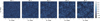 |
Fig. 1. Example of noisy convergence map, with five tomographic redshift bins, generating with sbi_lens's log-normal forward model. It is the fiducial map x0 used for benchmarking all the inference techniques. |
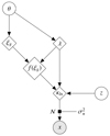 |
Fig. 2. Representation of sbi_lens's forward model used to generate log-normal convergence maps. |
Prior and fiducial values used for our inference benchmark.
2.3. LSST Y10 settings
According to the central limit theorem, we assume LSST Y10 observational noise to be Gaussian as we expect a high number of galaxies per pixel. Hence, the shear noise per pixel is given by a zero-mean Gaussian whose standard deviation is
 (10)
(10)
where σe = 0.26 is the per-component-shape standard deviation as defined in the LSST DESC Science Requirement Document (SRD, Mandelbaum et al. 2018), and Ns is the number of source galaxies per bin and pixel, computed using ngal = 27 arcmin−2 the galaxy number density (as in LSST DESC SRD) and Apix≈5.49 arcmin2 the pixel area. The convergence field is related to the shear field through the Kaiser Squires operator (Kaiser & Squires 1993). As this operator is unitary, it preserves the noise of the shear field; therefore, the convergence noise is also given by Eq. (10).
Our convergence map, x, is a 256×256 pixel map that covers an area of 10×10 deg2 in five tomographic redshift bins with an equal number of galaxies (see Fig. 3). The redshift distribution is modeled using the parametrized Smail distribution (Smail et al. 1995):
 (11)
(11)
with z0 = 0.11 and α = 0.68. We assume a photometric redshift error of σz = 0.05(1+z) (still according to LSST DESC SRD).
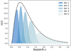 |
Fig. 3. LSST Y10 redshift distribution used in our forward model. |
3. Bayesian inference
In this section, we introduce our Bayesian inference framework enabling us to distinguish between implicit and explicit (full-field) inference more clearly in this paper.
Given a priori knowledge p(θ) about the parameters θ and information provided by data x linked to the parameters via the likelihood function p(x|θ), we are able to recover the parameters θ that might have led to this data. This is summarized by Bayes’ theorem:
 (12)
(12)
with p(θ|x) being the posterior distribution of interest and p(x) = ∫p(x|θ)p(θ)dθ the evidence. However, physical forward models are typically of the form p(x|θ,z), involving additional variables z known as latent variables. The presence of these latent variables makes the link between the data x and the parameters θ not straightforward, as x is now the result of a transformation involving the two random variables θ and z. Since the forward model depends on latent variables, we need to compute the marginal likelihood to perform inference; that is,
 (13)
(13)
which is typically intractable when z is of high dimension. As a result, the marginal likelihood p(x|θ) cannot be evaluated, and explicit inference techniques that rely on explicit likelihood such as the MCMC method or variational inference cannot be directly applied to the marginal likelihood p(x|θ). For this reason, this marginal likelihood is often assumed to be Gaussian, yielding an inaccurate estimation of the true posterior. Full-field inference instead aims to consider the exact distribution of the data x or the sufficient statistics t.
4. Inference quality evaluation
To quantify the quality of inference and thus benchmark all the inference algorithms, a performance metric has to be carefully chosen. Several metrics exist, each offering varying levels of precision, and they are usually chosen according to the knowledge we have about the true posterior (i.e., if we have access to the probability density function of the true distributions, its samples, or only the fiducial data or fiducial parameters). We took the 160 000 posterior samples obtained through explicit full-field inference as our ground truth and used the Classifier 2-Sample Tests (C2ST, Lopez-Paz & Oquab 2018). This decision is based on the understanding that the explicit full-field approach, which relies on sampling schemes, should theoretically converge to the true posterior distribution within the limit of a large number of samples. The convergence analysis of the MCMC, along with the large number of samples (160 000), indicates that the explicit, full-field inference posterior has converged. Additionally, we confirm this by visually comparing (in Fig. 4) the marginals of the fully converged samples obtained through explicit full-field inference (black) to the marginals of the posterior obtained through implicit inference (blue). Although we present implicit inference performed with only 1000 simulations in Fig. 4, it is worth noting that we ran the implicit inference method with over 1000 simulations, and it was consistently in agreement with this explicit posterior.
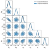 |
Fig. 4. From log-normal simulated LSST Y10-like convergence maps, we constrain wCDM parameters using two approaches: (1) the explicit full-field inference (black), obtained by sampling 160 000 posterior samples through an HMC scheme; and (2) the implicit full-field inference contours (blue), obtained by compressing the convergence maps into sufficient statistics using variation mutual information maximization (VMIM) and performing inference using NLE with 1000 simulations. We show three things: (1) implicit and explicit full-field inferences yield consistent constraints; (2) our implicit inference, when combined with an optimal compression procedure, allows full-field inference; (3) the C2ST metric indicates convergence when it is equal to 0.5 (see Sect. 4). However, when comparing explicit and implicit inference (which should theoretically yield the same posterior), we never reach this value, but rather we obtain 0.6. We justify that this value is acceptable and use it as a threshold for all benchmarked methods in this paper by showing that the marginals of the two approaches match, even though their C2ST is 0.6. |
We selected the C2ST metric due to its recognition as an effective and interpretable metric for comparing two distributions, particularly in the context of implicit inference. According to Lueckmann et al. (2021), C2ST outperforms other metrics such as the maximum mean discrepancy (MMD) and posterior predictive checks (PPCs) in various benchmarks. For instance, in the “Two Moons” benchmark task discussed by Lueckmann et al. (2021), C2ST demonstrated superior sensitivity to differences in distributions compared to MMD, which was found to be overly sensitive to hyperparameter choices. Furthermore, C2ST proved effective in scenarios involving multi-modal and complex posterior structures, where other metrics struggled to provide consistent and reliable results.
A two-sample test is a statistical method that tests whether samples X∼P and Y∼Q are sampled from the same distribution. For this, one can train a binary classifier f to discriminate between X (label 0) and Y (label 1) and then compute the C2ST statistic
![Mathematical equation: $$ {\hat {t}} = \frac {1}{N_{\mathrm {test}}} \sum _{i = 1}^{N_{\mathrm {test}}} {\mathbb {I}} \left [{\mathbb {I}} \left (f(z_i) >\frac {1}{2}\right ) = l_i \right ], $$](/articles/aa/full_html/2025/07/aa52410-24/aa52410-24-eq24.gif) (14)
(14)
where  and Ntest denotes the number of samples not used during the classifier training. If P=Q, the classifier fails to distinguish the two samples and thus the C2ST statistic remains at chance level (C2ST = 0.5). On the other hand, if P and Q are so different that the classifier perfectly matches the right label, C2ST = 1.
In practice, in our six-dimensional inference problem, we find this metric very sensitive, and the two distributions considered converged in Fig. 4 result in a C2ST of 0.6. Therefore, to make a fair comparison between all inference methods we benchmark all the methods with the same metric, the C2ST metric, and choose to fix a threshold of 0.6.
5. Explicit inference
5.1. Sampling the forward model
When the forward model is explicit, which means that the joint likelihood p(x|θ,z) can be evaluated, it is possible to sample it directly through an MCMC method, bypassing the computation of the intractable marginal likelihood p(x|θ).
Unlike sampling the marginal likelihood, this necessitates sampling both the parameters of interest θ as well as all latent variables z involved in the forward model,
 (15)
(15)
and marginalizing over the latent variables z afterward to obtain the posterior distribution p(θ|x).
As the latent variables are usually high-dimensional, they require a large number of sampling steps to make the MCMC converge. Therefore, Hamilton Monte Carlo (HMC, Neal 2011; Betancourt 2018), which can efficiently explore the parameter space thanks to gradient information, is usually used for such high-dimensional posteriors. However, this requires the explicit likelihood to be differentiable.
We note that for each step the forward model needs to be called, which can make this approach costly in practice as generating one simulation can take a very long time. This would also be true in cases where the marginal likelihood can be evaluated, but since the latent variables z do not have to be sampled, the parameter space is smaller and the MCMC does not need as many steps.
5.2. Explicit full-field inference constraints
sbi_lens’ differentiable joint likelihood is
 (16)
(16)
with κln being the convergence map that depends on the cosmology θ and the latent variables z. Given that the observational noise is uncorrelated across tomographic redshift bins and pixels, we can express the log-likelihood of the observed data x0 as
![Mathematical equation: $$ {\cal {{L}}}(\theta , z) = {\mathrm {constant}} - \sum _i^{N_{\mathrm {pix}}} \sum _{j}^{N_{\mathrm {bins}}} \frac {\left [\kappa _{ln}^{i,j}(\theta , z)-x_0^{i,j}\right ]^2}{2\sigma _n^2}\cdot $$](/articles/aa/full_html/2025/07/aa52410-24/aa52410-24-eq28.gif) (17)
(17)
By construction, p(z|θ) is independent of the cosmology θ; hence, the log posterior we aim to sample is
 (18)
(18)
with p(z) being a reduced-centered Gaussian and p(θ) as in Table 1. We used an HMC scheme to sample Eq. (18). Specifically, we used the No-U-Turn sampler (NUTS, Hoffman & Gelman 2014) from NumPyro (Phan et al. 2019; Bingham et al. 2019), which efficiently proposes new relevant samples using the derivatives of the distribution we sampled from, namely ∇θ,zlog p(θ,z|x=x0).
Given the fixed observed convergence map x0, Fig. 4 shows the posterior constraints on Ωc,Ωb,σ8,ns,w0,h0. As explained in Sect. 4, we consider this posterior of 160 000 samples converged as it yields the same constraint as our implicit full-field approach. Therefore, we consider these 160 000 samples as our ground truth.
5.3. Number of simulations for explicit full-field inference
We conducted a study to access the minimum number of simulations needed to achieve a good approximation of posterior distribution p(θ|x=x0). In other words, we tried to access the minimum number of simulations needed to have converged MCMC chains and a good representation of the posterior distribution.
Since there is no robust metric to estimate the convergence of MCMCs, and because we aim to compare all inference methods with the same metric, we used the C2ST metric to access the minimum number of simulations required to have converged chains. We proceed as follows: given the fully converged chains of 160 000 posterior samples from Fig. 4, for each number of simulation N, we took the first N samples and computed the C2ST metric comparing those samples to the 160 000 ones from the fully converged chains. The C2ST metric is based on the training of a classifier to distinguish between two populations under the cross-entropy loss and thus requires an equal number of samples of the two distributions. We used a kernel density estimator (KDE) (Parzen 1962) to fit the samples, enabling us to generate the required number of samples to compare the two distributions. We note that KDEs, Gaussian filters, or smoothing are always used to visualize distribution samples using contour plots, thus motivating our approach. In addition, the distribution of interest is a six-dimensional unimodal and almost Gaussian distribution, making it easy to fit through a KDE. We used a Gaussian kernel and adjusted the bandwidth to align with the contour plots shown by GetDist, as highlighted in Fig. E.7.
We note that samples and simulations are not the same thing. During each step, the proposal of the MCMC suggests a pair of parameters θ1 and z1 and produces a corresponding simulation x∼p(x|θ=θ1,z=z1). The MCMC keeps only the parameters θ1 and z1 if it yields a plausible x according to the likelihood function evaluated on the observation x0, and plausible θ1 and z1 according to their priors. The sample is the pair θ and z that is kept by the MCMC. Specifically, to obtain one posterior sample using the NUTS algorithm, we need 2×N simulations, with N denoting the number of leapfrog steps. Indeed, the proposal of HMC methods is based on Hamiltonian equations that are discretized using the leapfrog integrator:
 (19)
(19)
 (20)
(20)
 (21)
(21)
with ϵ being the step size and M the mass matrix, αt corresponding to the position of (θ,z) at time t, and rt denoting the values of the random momentum at time t∈[0,N]. After N leapfrog steps, the total number of log probability evaluations is N. As each gradient requires the cost of two simulations (one to evaluate the primal values during the forward pass and one to evaluate gradients backward in the reverse mode of automatic differentiation), the total number of simulations is 2×N. In our case, we find that the NUTS algorithm requires 2×(26−1) = 126 simulations (always reaching the maximum depth of the tree that is set to 6) to generate one sample.
Figure 5 shows the convergence results of our explicit full-field inference as a function of the number of simulations and the effective sample size. According to the threshold of C2ST = 0.6 that we mention in Sect. 4, this study suggests that 630 000 simulations for our sampler corresponding to 400 independent samples are enough to have converged MCMC chains. The number of independent samples is estimated using the effective-sample-size (ess) lower-bound estimate from TensorFlow Probability (Dillon et al. 2017). In addition, Fig. E.6 shows the explicit posterior constraints obtained for different simulation budgets, and Fig. E.5 shows the evolution of the mean and standard deviation of the posteriors as a number of simulations. We note that the C2ST metric is sensitive to higher order correlations, but if one only cares about marginals, the explicit inference posterior can be considered converged with only 63 000 simulations (corresponding to 24 independent samples), as shown by the combination of contour plots Figs. E.6 and E.5.
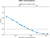 |
Fig. 5. Explicit full-field inference: quality of cosmological posterior approximation as a function of the number of simulations used and effective sample size. The dashed line indicates the C2ST threshold of 0.6, marking the point at which the posterior is considered equal to the true distribution (see Sect. 4). |
These results are not a strong statement about explicit inference in general as we do not investigate other sampling schemes and preconditioning schemes (this study is left for future work). However, the NUTS algorithm is one of the state-of-the-art samplers and has already been used in various full-field studies (e.g. Zhou et al. 2024; Boruah et al. 2024). However, it is important to note that there are other powerful HMC schemes, such as the Microcanonical Langevin Monte Carlo (MCLMC) method (Robnik et al. 2023), which might perform well with fewer simulations and has also been used in full-field studies (Bayer et al. 2023). Regardless of the sampling scheme used, we suggest that readers refer to the effective sample size values to translate the results to their sampler.
6. Implicit inference
Although explicit full-field inference offers a promising framework for performing rigorous Bayesian inference, it comes with the downside of requiring an explicit likelihood. Additionally, sampling from the joint likelihood even with HMC schemes can be very challenging and requires a large number of simulations. Instead, implicit inference has emerged as a solution to tackle the inference problem without relying on an explicit likelihood. These techniques rely on implicit likelihoods, which are more commonly known as simulators. A simulator is a stochastic process that takes as input the parameter space θ∼p(θ) and returns a random simulation x. It does not require the latent process of the simulator to be explicit.
Comparably to sampling the forward model, given an observation x0, one can simulate a large range of θi and accept the parameters that verify |xi−x0|<ϵ with ϵ a fixed threshold to build the posterior p(θ|x=x0). This is the idea behind the approximate Bayesian computation (ABC) method (e.g., Rubin 1984; Beaumont et al. 2002; Sisson et al. 2018). This method used to be the traditional way to carry out implicit inference, but its poor scalability with dimension encouraged the community to develop new techniques. In particular, the introduction of machine learning leading to neural implicit inference methods has been shown to perform better. These neural-based methods cast the inference problem into an optimization task, where the goal is to find the set of parameters φ so that the neural parametric model best describes the data. Then, the posterior is approximated using this surrogate model evaluated on the given observation.
Implicit inference has already been successfully applied to cosmic shear analyses. For instance, Lin et al. (2023) and von Wietersheim-Kramsta et al. (2025) applied it to two-point statistics rather than using the standard explicit inference method assuming a Gaussian likelihood. Similarly, to bypass this traditional Gaussian likelihood assumption, Jeffrey et al. (2024) applied implicit inference to the power spectra, peak counts, and neural summary statistics.
In this section, we introduce the NLE method and its augmented version with gradient ∂NLE, and we present the benchmark results. The neural ratio estimation (NRE), neural posterior estimation (NPE), and sequential methods are described in Appendix B.1; and the benchmark results of (S)NLE, (S)NPE, and (S)NRE can be found in Appendix B.3. In this section, we focus our study on the NLE method as our comparison of the three main implicit inference methods (see Fig. B.1) suggests that NLE and NPE are the ones that perform the best. We chose not to use the NPE method, as the augmented gradient version of NPE (Zeghal et al. 2022) requires specific neural architectures that proved to be more costly simulation-wise.
6.1. Learning the likelihood
The aim of the NLE method is to learn the marginal likelihood pφ(x|θ) from a set of parameters and corresponding simulations (θ,x)i = 1..N. Thanks to the development of new architectures in the neural density estimator field, this can be achieved by using conditional normalizing flows (NFs) (Rezende & Mohamed 2015). Conditional NFs are parametric models pφ that take (θ,x) as input and return a probability density pφ(x|θ), which can be evaluated and/or sampled. To find the optimal parameters  that make pφ(x|θ) best describe the data, one trains the NF so that the approximate distribution pφ(x|θ) is the closest to the unknown distribution p(x|θ). To quantify this, we used the forward Kullback-Leibler divergence DKL(.||.). The DKL is positive and equal to zero if and only if the two distributions are the same, motivating the following optimization scheme:
![Mathematical equation: $$ {\hat {\varphi }} = \arg \min _{\varphi } {\mathbb {E}}_{p(\theta )} \left [D_{KL}(p(x | \theta ) \; || \; p_{\varphi }(x | \theta )) \right ] $$](/articles/aa/full_html/2025/07/aa52410-24/aa52410-24-eq34.gif) (22)
(22)
![Mathematical equation: $$ \begin{aligned}& = \arg \min _{\varphi } {\mathbb {E}}_{p(\theta )} \left [{\mathbb {E}}_{p(x | \theta )}\Big [\log \left (\frac {p(x | \theta )}{p_{\varphi }(x | \theta )}\right ) \Big ] \right ] \\ & = \arg \min _{\varphi } \mathop {\underbrace {{\mathbb {E}}_{p(\theta )} \left [{\mathbb {E}}_{p(x | \theta )}\left [\log \left (p(x | \theta )\right ) \right ] \right ]}}\limits _{{\mathrm {constant\ w.r.t}}\ \varphi } \\ & \qquad - {\mathbb {E}}_{p(\theta )} \left [{\mathbb {E}}_{p(x | \theta )}\left [\log \left (p_{\varphi }(x | \theta )\right ) \right ] \right ] \\ & = \arg \min _{\varphi } - {\mathbb {E}}_{p(\theta )} \left [{\mathbb {E}}_{p(x | \theta )}\left [\log \left (p_{\varphi }(x | \theta )\right ) \right ] \right ], \end{aligned} $$](/articles/aa/full_html/2025/07/aa52410-24/aa52410-24-eq35.gif)
leading to the loss
![Mathematical equation: $$ {\cal {{L}}} = {\mathbb {E}}_{p(\theta , x)} \left [- \log p_{\varphi } (x | \theta ) \right ], $$](/articles/aa/full_html/2025/07/aa52410-24/aa52410-24-eq36.gif) (23)
(23)
which does not require evaluation of the true target distribution p(x|θ) anymore. To compute this loss, only a set of simulations (θ,x)∼p(θ,x) obtained by first generating parameters from the prior θi∼p(θ) and then generating the corresponding simulation xi∼p(x|θ=θi) through the simulator are needed. We note that the approximated likelihood, under the loss of Eq. (23), is learned for every combination (θ,x)∼p(x,θ) at once.
Given observed data x0, the approximated posterior  is then obtained by using an MCMC with the following log probability:
  . This MCMC step makes NLE (and NRE) less amortized and slower than the NPE method, which directly learned the posterior distribution pφ(θ|x) for every pair (θ,x)∼p(x,θ) and only needs to be evaluated on the desire observation x0 to obtain the approximated posterior pφ(θ|x=x0). However, it is less challenging than using an MCMC scheme to sample the forward model in the explicit inference framework. Indeed, now one only has to sample the learned marginal likelihood pφ(x|θ) (or learned likelihood ratio), not the joint likelihood of the forward model p(x|θ,z).
6.2. NLE augmented with gradients
Although there are methods to reduce the number of simulations, such as sequential approaches (see Appendix B), they still treat the simulator as a black box. As underlined by Cranmer et al. (2020), the emergence of probabilistic programming languages makes it easier to open this black box (making the implicit likelihood explicit) and extract additional information such as the gradient of the simulation. In particular, Brehmer et al. (2020) noticed that they can compute the joint score ∇θlog p(x,z|θ) as the sum of the scores of all the latent transformations encountered in the differentiable simulator:
 (24)
(24)
 (25)
(25)
The most important result is that through the use of the classical mean-squared error (MSE) loss (also known as score matching (SM) loss),
![Mathematical equation: $$ {\cal {{L}}}_{\mathrm {SM}} = {\mathbb {E}}_{p(x,z,\theta )} \left [\parallel \nabla _{\theta } \log p(x,z | \theta ) - \nabla _\theta \log p_\varphi (x | \theta ) \parallel _2^2 \right ], $$](/articles/aa/full_html/2025/07/aa52410-24/aa52410-24-eq41.gif) (26)
(26)
they showed how to link this joint score to the intractable marginal score ∇θlog p(x |θ). As explained in Appendix C, ℒSM is minimized by ![Mathematical equation: $ {\mathbb {E}}_{p(z |x,\theta )} \left [\nabla _{\theta } \; \log \; p(x, z |\theta ) \right ] $](/articles/aa/full_html/2025/07/aa52410-24/aa52410-24-eq42.gif) and can be derived as
and can be derived as
![Mathematical equation: $$ \begin{aligned}& {\mathbb {E}}_{p(z |x,\theta )} \left [\nabla _{\theta } \; \log \; p(x, z |\theta ) \right ] \\ & = {\mathbb {E}}_{p(z |x,\theta )} \left [\nabla _{\theta } \; \log \; p(z|x, \theta ) \right ] + \nabla _{\theta } \; \log \; p(x | \theta ) \\ & = {\mathbb {E}}_{p(z| x,\theta )} \left [\frac { \nabla _{\theta } \; p(z|x, \theta )} {p(z|x, \theta )} \right ] + \nabla _{\theta } \; \log \; p(x | \theta ) \\ & = \int \nabla _{\theta } \; p(z|x, \theta ) \; dz + \nabla _{\theta } \; \log \; p(x | \theta ) \\ & = \nabla _{\theta } \; \int p(z|x, \theta ) \; dz + \nabla _{\theta } \; \log \; p(x | \theta ) \\ & = \nabla _{\theta } \; \log \; p(x | \theta ). \end{aligned} $$](/articles/aa/full_html/2025/07/aa52410-24/aa52410-24-eq43.gif) (27)
(27)
This loss learns how the probability of x given θ changes according to θ and thus can be combined with the traditional negative log-likelihood loss (Eq. (13)) to help the neural density estimator learn the marginal likelihood with fewer simulations. The NF now learns pφ(x|θ) from (θ,x,∇θlog p(x,z|θ))i = 1..N under the combined loss,
 (28)
(28)
with λ being a hyper-parameter that has to be fined-tuned according to the task at hand. Brehmer et al. (2020) called this method the SCore-Augmented Neural Density Approximates Likelihood (SCANDAL); we choose to rename it ∂NLE for clarity in our paper. Equivalently, other quantities such as the joint likelihood ratio r(x,z|θ0,θ1) = p(x,z|θ0)/p(x,z|θ1) and the joint posterior gradients ∇θlog p(θ|x,z) can be used to help learn the likelihood ratio (Brehmer et al. 2020) and the posterior (Zeghal et al. 2022) respectively.
6.3. Compression procedure
In this section, we provide a brief summary of the compression procedure we performed to build sufficient statistics. A more detailed description and comparison of compression procedures applied in the context of weak-lensing, full-field implicit inference can be found in Lanzieri et al. (2025).
Based on the benchmark results of Lanzieri et al. (2025), we chose to use the variational mutual information maximization (VMIM, Jeffrey et al. 2021) neural compression. This compression builds summary statistics t=Fφ(x) by maximizing the mutual information I(t,θ) between the parameters of interest θ and the summary statistics t. More precisely, the mutual information is defined as
![Mathematical equation: $$ I(t, \theta ) = {\mathbb {E}}_{p(t, \theta )} [\log {p(\theta | t)}]- H(\theta ), $$](/articles/aa/full_html/2025/07/aa52410-24/aa52410-24-eq45.gif) (29)
(29)
where H denotes the entropy. Replacing the summary statistics t by the neural network Fφ and the intractable posterior p(θ|t) by a variational distribution pψ(θ|t) to be optimized jointly with the compressor, we obtain the following variational lower bound (Barber & Agakov 2003):
![Mathematical equation: $$ I(t, \theta ) \geq {\mathbb {E}}_{p(x, \theta )} [\log {p_\psi (\theta \; | \;F_\varphi (x))}]- H(\theta ). $$](/articles/aa/full_html/2025/07/aa52410-24/aa52410-24-eq46.gif) (30)
(30)
Hence, by training the neural network Fφ jointly with a variational distribution (typically a NF) pψ under the loss
![Mathematical equation: $$ {\cal {{L}}}_{{\mathrm {VMIM}}} = - {\mathbb {E}}_{p(x, \theta )} [\log {p_\psi (\theta \; | \;F_\varphi (x))}], $$](/articles/aa/full_html/2025/07/aa52410-24/aa52410-24-eq47.gif) (31)
(31)
we were able, by construction and within the limit of the flexibility of Fφ and pψ, to build summary statistics t that contain the maximum amount of information regarding θ that is embedded in the data x. As equality is approached, the maximization of the mutual information yields sufficient statistics such that p(θ|x) = p(θ|t).
As proof that in our particular case, these summary statistics extract all the information embedded in our convergence maps, and thus are sufficient statistics, we show in Fig. 4 that the contours obtained using this compression and the NLE implicit inference technique allowed us to recover the explicit full-field constraints.
We used 100 000 simulations for the compression part and did not investigate the question of the minimum number of simulations required. Although we used a large number of simulations to train our compressor, we can produce near-optimal summary statistics without training a neural network, which eliminates the need for additional simulations. As an example, Cheng et al. (2020) showed that they can produce summary statistics using scattering transforms that result in constraints similar to those obtained by building summary statistics using a CNN trained under mean-absolute-error (MAE) loss. While it is not guaranteed that these scattering transform coefficients will provide sufficient statistics to perform full-field inference, we hope that advances in transfer learning will allow us to propose new compression schemes that need very few simulations. This is left for future work. Details regarding our compressor architecture can be found in Appendix D.1.
6.4. Results
For this study, we used the NLE algorithm as in Papamakarios et al. (2018). And use the ∂NLE method introduced by Brehmer et al. (2020) to leverage gradient information. All approaches share the same NF architecture and sampling scheme (all details can be found in Appendix D.3).
We benchmark the previously presented implicit inference methods on our sbi_lens's log-normal LSST Y10-like forward model. The goal of this inference problem is to constrain the following cosmological parameters: Ωc,Ωb,σ8,ns,w0,h0 given a fiducial convergence map x0. Our fiducial map x0 is the same for all the benchmarked methods in the paper.
This benchmark aims to find the inference method that can achieve a given posterior quality (C2ST = 0.6) with the minimum number of simulations; for this, the procedure is the following:
-
Starting from the entire dataset, we compress the tomographic convergence maps x of 256×256×5 pixels into six-dimensional sufficient statistics. We use the VMIM neural compression as described in Sect. 6.3.
-
From this compressed dataset, we then pick a number of simulations and approximate the posterior distribution using NLE and ∂NLE methods.
-
Then, we evaluate the approximated posterior against the fully converged explicit full-field posterior (our ground truth) using the C2ST metric.
The C2ST convergence results are displayed in Fig. 6. In the appendix, we provide additional convergence results. Fig. E.1 shows the posterior contours’ evolution obtained through NLE, and Figs. E.2, E.3, E.4 depict the evolution of the mean and standard deviation of the approximated posterior as a number of simulations.
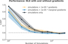 |
Fig. 6. Implicit inference augmented with gradients: quality of the cosmological posterior approximation as a function of the number of simulations used. We compare three methods: (1) ∂NLE with the gradients of the simulator ∇θlog p(x,z|θ) (yellow); (2) ∂NLE with marginal gradients ∇θlog p(x|θ) (blue); and (3) the classical NLE method (black). The dashed line indicates the C2ST threshold of 0.6, marking the point at which the posterior is considered equal to the true distribution (see Sect. 4). We show that the gradients provided by the simulator (yellow curve) do not help reduce the number of simulations as they are too noisy (see Fig. 7). |
We find that unlike previous results (Brehmer et al. 2020; Zeghal et al. 2022), the gradients ∇θlog p(x,z|θ) do not provide additional information enabling a reduction in the number of simulations. Indeed, Fig. 6 shows similar convergence curves for the ∂NLE method (yellow) and the NLE method (black). This issue arises as we attempt to constrain the gradients of the learned marginal distribution pφ(x|θ) by using the joint gradients ∇θlog p(x,z|θ) from the simulator. Indeed, the benefit of these joint gradients depends on their “level of noise”. In other words, their benefit depends on how much they vary compared to the marginal gradients. To visually exhibit this gradient stochasticity, we considered the gradients of a two-dimensional posterior ∇θlog p(θ|x) and the joint gradients ∇θlog p(θ|x,z) provided by the simulator. By definition, the gradients should align with the distribution, as seen in the left panel of Fig. 7. As demonstrated in the middle panel of Fig. 7, the gradients we obtain from the simulator are directed toward p(θ|x,z), which differs from p(θ|x) = ∫p(θ|x,z)p(z|x)dz. The stochasticity of the gradients relies on the standard deviation of p(z|x) and how much p(θ|x,z) “moves” according to z. As a result, instead of the gradients field displayed in the left panel of Fig. 7, we end up with the gradients field depicted in the right panel.
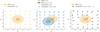 |
Fig. 7. Illustration of gradient stochasticity. The left panel shows a 2D posterior distribution p(θ|x=x0) evaluated at the observed data x0 and its gradients ∇θlog p(θ|x=x0). The middle panel shows the difference between the posterior p(θ|x=x0) (yellow) and the joint posterior p(θ|x=x0,z=z0) (blue) with z0 a latent variable that leads to x0. The yellow arrows correspond to the gradients of the posterior, and the blue ones to the gradients of the joint posterior. The right panel displays the gradient field that we obtained in practice from the simulator. Each gradient aligns with its corresponding joint posterior, resulting in a “noisy” gradient field compared to that of the posterior (first panel). |
To confirm this claim, we learn from the simulator's gradients, ∇θlog p(x,z|θ), and the marginal ones, ∇θlog p(x|θ). For this, we used a neural network (the architecture can be found in Appendix D.2) that we trained under the following MSE loss function:
![Mathematical equation: $$ {\cal {{L}}}_{\mathrm {MarginalSM}} = {\mathbb {E}}_{p(x,z,\theta )} \left [\parallel \nabla _{\theta } \log p(x,z | \theta ) - g_\varphi (x,\theta ) \parallel _2^2 \right ]. $$](/articles/aa/full_html/2025/07/aa52410-24/aa52410-24-eq48.gif) (32)
(32)
This loss is almost the same as Eq. (26), except that instead of using an NF to approximate ∇θlog p(x|θ) and then take its gradients, we trained a neural network to approximate the gradient values given θ and x. This loss is minimized by gφ(x,θ) = ∇θlog p(x|θ) (as explained in Sect. 6.2), allowing us to learn the intractable marginal gradients from simulations.
We then used these marginal gradients in the ∂NLE method (blue curve) and show that those gradients help reduce the number of simulations. What we demonstrate here is that the stochasticity of our LSST Y10-like simulator dominates the gradient information, and thus the ∂NLE method does not help perform inference with fewer simulations.
We could have used a method to denoise the gradients. Specifically, Millea & Seljak (2022) introduced marginal unbiased score expansion (MUSE), a way of computing marginal gradients from simulations, and proposed a frequentist and Bayesian approach for parameter inference that leverages this quantity. In our case, the ∂NLE with marginal gradients converges with ∼400 simulations, while ∂NLE with gradients from the simulator converges with twice as many simulations. Hence, to be beneficial, computing the marginal gradient should take fewer than two simulations, which is not feasible with MUSE as it requires at least ten simulations to have an “acceptable” estimation of the marginal gradient (Millea & Seljak 2022).
7. Conclusion and discussion
Full-field inference is the optimal form of inference as it aims to perform inference without any loss of information. This kind of inference is based on a simulation model known as a simulator, forward model, or Bayesian hierarchical model in cases where the model is hierarchical. There are two ways of conducting full-field inference from this forward model: through explicit or implicit inference. The first way can be applied when the forward model is explicit. This means that the field-based joint likelihood p(x=x0|θ,z) can be evaluated and thus sampled through sampling schemes such as MCMC. The second one can be used when only simulations are available; in this case, it is said that the likelihood is implicit. While it is possible to perform implicit inference directly at the pixel level by feeding the maps to the neural density estimator (Dai & Seljak 2024), it is usually more robust and safe to break it down into two steps: first performing a lossless compression, and second performing the implicit inference on these sufficient statistics. Specifically, in this work, sufficient statistics are built using an optimal neural-based compression based on the maximization of the mutual information I(θ,t) between the cosmological parameters θ and the summary statistics t. However, other compression schemes, requiring fewer or zero simulations, could be used while still offering very good quality summary statistics (Cheng et al. 2020). Additionally, the advent of transfer learning could offer a way of performing compression with fewer simulations; this is left for future work.
This work aimed to find which full-field inference methods require the minimum number of simulations and if differentiability is useful for implicit full-field inference. To answer these questions, we introduced a benchmark that compares various methods to perform weak lensing full-field inference. For our benchmark, we used sbi_lens's differentiable forward model, which generates log-normal convergence maps imitating a simplified version of the LSST Y10 quality. We evaluated the performance of several inference strategies by evaluating the constraints on (Ωc,Ωb,σ8,h0,ns,w0), specifically using the C2ST metric.
We found the following results:
-
Explicit and implicit full-field inference yield the same constraints. However, according to the C2ST metric and the threshold of C2ST = 0.6, the explicit full-field inference requires 630 000 simulations (corresponding to 400 independent samples). In contrast, the implicit inference approach requires 101 000 simulations split into 100 000 simulations for compression and 1000 for inference. We note that we arbitrarily used 100 000 simulations for the compression part and did not explore the question of performing compression with a minimum number of simulations. Hence, 101 000 simulations is an upper bound of the number of simulations actually required to perform implicit full-field inference in this particular problem.
-
The C2ST is sensitive to higher order correlations that one cannot see by looking at the marginals or first moments, making it a good metric for comparing distributions. However, as we are mostly interested in those marginals, it is worth noting that by looking at the combination of contour plots from Fig. E.6 and first-moments convergence plots from Fig. E.5, the explicit inference can be considered “converged” with 63 000 simulations (corresponding to 24 independent samples), as emphasized by Fig. E.6, which correspond to C2ST = 0.76 and the implicit inference performed through NLE with 101 000 (1000 for inference and 100 000 to build sufficient statistics) as shown in Fig. 4 which corresponds to C2ST = 0.6.
-
For implicit inference, we exploited the simulator's gradient using the SCANDAL method proposed by Brehmer et al. (2020). Our study indicates that the gradients contain a significant noise level due to the latent variable's behavior, which makes it difficult to achieve convergence with fewer simulations. We note that the effectiveness of such gradient-based methods depends on the specific problem at hand. These methods can still be useful in scenarios where the noise level is not significant. This has been demonstrated in studies such as Brehmer et al. (2020) and Zeghal et al. (2022). It is also important to keep in mind that there may be other ways to leverage the differentiability of simulators and encourage further research in this area. Finally, we note that methods to denoise the gradients exist (Millea & Seljak 2022), but, in our specific case, the gain compared to the number of simulations that this method requires is not significant.
It is worth noting that for each explicit inference simulation budget, the C2ST is calculated against fully converged explicit inference samples, resulting in a value that can reach almost 0.5. For implicit inference, the C2ST is also computed against the fully converged explicit inference samples. Both methods should produce the same constraints, but due to slight differences in the posterior approximation, the C2ST cannot go below 0.6. Hence, we consider a value of 0.6 as indicating convergence (see Fig. 4).
It is important to mention that in most real-world physical inference problems, such a metric cannot be used as it requires a comparison of the approximated posterior to the true one. Instead, for implicit inference, coverage tests (Lemos et al. 2023) should be used to assess the quality of the posterior. For explicit full-field inference, although diagnostics exist, it is very difficult to verify if the MCMC has explored the entire space. If possible, the safest option would be to compare the two full-field approaches, as they should yield the same posterior. Implicit inference is likely the easiest to use in such a scenario because it does not require the modeling of the very complicated latent process of the forward model and can be performed even in multimodal regimes; whereas, explicit inference has to sample the latent process of the forward model, and the more dimensions there are, the more time it needs to explore the entire parameter space. In addition, it can fail in the case of multimodal distribution as it can stay stuck in local maxima and never converge. However, for implicit inference, too few simulations can result in an overconfident posterior approximation, as shown in Fig. E.1. Therefore, within the limit of a reasonable number of simulations, the implicit inference method should be the easiest to use.
Finally, we discuss several limitations of our approach. Although the current setup is not fully realistic for LSST, this minimalist approach was deliberately chosen to benchmark explicit and implicit inference within a manageable time frame. It is important to note that we used log-normal simulations instead of more computationally intensive N-body PM simulations. While this model accounts for additional non-Gaussianity (as illustrated in Fig. A.1), it does not match the complexity of N-body simulations. Modeling systematics at the field-level likelihood is inherently complex and poses challenges for implementing explicit inference. Similarly, incorporating other forms of noise and masking at the field level may be difficult. To ensure a fair comparison, we opted not to include these complexities, which enabled us to use the same simulator for both inference methods to maintain consistency across the comparison. While it is true that an incorrect forward model would impact the results when applying this framework to real observations, we do not expect our conclusions to change regarding the comparison of implicit and explicit inference. However, it will be interesting to validate this assumption with a more realistic gravity model in future work. The results presented here should be viewed as illustrative benchmarks rather than definitive predictions for LSST data, though we remain optimistic that our findings will be relevant for realistic weak lensing inference.
The explicit inference results are not a strong statement, as we did not explore other sampling and preconditioning schemes (which is left for future work). Our sampler choice for the benchmark was motivated by the fact that the NUTS algorithm is a state-of-the-art sampler and has been extensively used in full-field studies (Zhou et al. 2024; Boruah et al. 2024). However, there are other sampling schemes, such as powerful microcanonical Langevin Monte Carlo (MCLMC) methods (Robnik et al. 2023) which might require fewer simulations and have been applied in full-field studies (Bayer et al. 2023). Meanwhile, we recommend that the reader refer to the effective sample size values to translate the results to their sampler.
We used the NLE implicit method for our study as, regarding our benchmark results of Fig. B.1, it seems to be the one that performs the best. NPE provides comparable results, but necessitates using the ∂NPE method of Zeghal et al. (2022) to leverage gradient information. Since the NPE method aims to learn the posterior directly, this method requires the NF to be differentiable. However, the smooth NF architecture (Köhler et al. 2021) that Zeghal et al. (2022) used was too simulation-expensive for our needs. We also experimented with continuous normalizing flows trained under negative log-likelihood loss, but found that it took a very long time to train.
Acknowledgments
This paper has undergone internal review in the LSST Dark Energy Science Collaboration. The authors would like to express their sincere gratitude to the internal reviewers, Alan Heavens and Adrian Bayer, for their valuable feedback, insightful comments, and suggestions, which helped to significantly improve the quality of this work. They also extend their thanks to Benjamin Remy for his contributions through countless discussions and helpful comments on the paper. Additionally, they appreciate the constructive feedback provided by Martin Kilbinger and Sacha Guerrini. JZ led the project, contributed to brainstorming, developed the code, and wrote the paper. DL contributed to brainstorming and code development, particularly in developing the forward model, and reviewed the paper. FL initiated the project and contributed through mentoring, brainstorming, code development, and paper reviews. AB contributed mentoring, brainstorming, code development, and paper reviews. GL and EA provided mentoring, participated in brainstorming, and contributed to reviewing the paper. AB contributed to the review of the paper and participated in brainstorming the metric used for explicit inference. The DESC acknowledges ongoing support from the Institut National de Physique Nucléaire et de Physique des Particules in France; the Science & Technology Facilities Council in the United Kingdom; and the Department of Energy, the National Science Foundation, and the LSST Corporation in the United States. DESC uses resources of the IN2P3 Computing Center (CC-IN2P3–Lyon/Villeurbanne - France) funded by the Centre National de la Recherche Scientifique; the National Energy Research Scientific Computing Center, a DOE Office of Science User Facility supported by the Office of Science of the U.S. Department of Energy under Contract No. DE-AC02-05CH11231; STFC DiRAC HPC Facilities, funded by UK BEIS National E-infrastructure capital grants; and the UK particle physics grid, supported by the GridPP Collaboration. This work was performed in part under DOE Contract DE-AC02-76SF00515. This work was supported by the Data Intelligence Institute of Paris (diiP), and IdEx Université de Paris (ANR-18-IDEX-0001). This work was granted access to the HPC/AI resources of IDRIS under the allocations 2023-AD010414029 and AD011014029R1 made by GENCI. This work used the following packages: Numpy (Harris et al. 2020), NumPyro (Phan et al. 2019), JAX (Bradbury et al. 2018), Haiku (Hennigan et al. 2020), Optax (DeepMind et al. 2020), JAX-COSMO (Campagne et al. 2023), GetDist (Lewis 2019), Matplotlib (Hunter 2007), CosMomentum (Friedrich et al. 2020), scikit-learn (Pedregosa et al. 2011), TensorFlow (Abadi et al. 2016), TensorFlow Probability (Dillon et al. 2017), sbi (Tejero-Cantero et al. 2020) and sbibm (Lueckmann et al. 2021).
Figure A.1 quantifies the amount of non-Gaussianities in our model compared to Gaussian simulations.
References
- Abadi, M., Agarwal, A., Barham, P., et al. 2016, arXiv e-prints [arXiv:1603.04467] [Google Scholar]
- Aihara, H., Arimoto, N., Armstrong, R., et al. 2017, PASJ, 70, S4 [NASA ADS] [Google Scholar]
- Ajani, V., Peel, A., Pettorino, V., et al. 2020, Phys. Rev. D, 102, 103531 [Google Scholar]
- Akhmetzhanova, A., Mishra-Sharma, S., & Dvorkin, C. 2024, MNRAS, 527, 7459 [Google Scholar]
- Alsing, J., Heavens, A., Jaffe, A. H., et al. 2016, MNRAS, 455, 4452 [Google Scholar]
- Alsing, J., Heavens, A., & Jaffe, A. H. 2017, MNRAS, 466, 3272 [Google Scholar]
- Barber, D., & Agakov, F. 2003, in Advances in Neural Information Processing Systems, eds. S. Thrun, L. Saul, & B. Schölkopf (MIT Press), 16 [Google Scholar]
- Bayer, A. E., Seljak, U., & Modi, C. 2023, arXiv e-prints [arXiv:2307.09504] [Google Scholar]
- Beaumont, M. A., Zhang, W., & Balding, D. J. 2002, Genetics, 162, 2025 [Google Scholar]
- Betancourt, M. 2018, arXiv e-prints [arXiv:1701.02434] [Google Scholar]
- Bingham, E., Chen, J. P., Jankowiak, M., et al. 2019, J. Mach. Learn. Res., 20, 28:1 [Google Scholar]
- Blum, M. G. B., & François, O. 2009, Stat. Comput., 20, 63 [Google Scholar]
- Böhm, V., Hilbert, S., Greiner, M., & Enßlin, T. A. 2017, Phys. Rev. D, 96, 123510 [CrossRef] [Google Scholar]
- Boruah, S. S., Fiedorowicz, P., & Rozo, E. 2024, Phys. Rev. D, submitted [arXiv:2403.05484] [Google Scholar]
- Bradbury, J., Frostig, R., Hawkins, P., et al. 2018, JAX: composable transformations of Python+NumPy programs, http://github.com/google/jax [Google Scholar]
- Brehmer, J., Louppe, G., Pavez, J., & Cranmer, K. 2020, PNAS, 117, 5242 [Google Scholar]
- Campagne, J. -E., Lanusse, F., Zuntz, J., et al. 2023, Open J. Astrophys., 6 [Google Scholar]
- Charnock, T., Lavaux, G., & Wandelt, B. D. 2018, Phys. Rev. D, 97, 083004 [NASA ADS] [CrossRef] [Google Scholar]
- Cheng, S., Ting, Y. -S., Ménard, B., & Bruna, J. 2020, MNRAS, 499, 5902 [Google Scholar]
- Clerkin, L., Kirk, D., Manera, M., et al. 2017, MNRAS, 466, 1444 [NASA ADS] [CrossRef] [Google Scholar]
- Cranmer, K., Pavez, J., & Louppe, G. 2015, arXiv e-prints [arXiv:1506.02169] [Google Scholar]
- Cranmer, K., Brehmer, J., & Louppe, G. 2020, PNAS, 117, 30055 [NASA ADS] [CrossRef] [Google Scholar]
- Dai, B., & Seljak, U. 2024, PNAS, 121, e2309624121 [Google Scholar]
- Dax, M., Wildberger, J., Buchholz, S., et al. 2023, arXiv e-prints [arXiv:2305.17161] [Google Scholar]
- de Jong, J. T. A., Kleijn, G. A. V., Kuijken, K. H., & Valentijn, E. A. 2012, Exp. Astron., 35, 25 [Google Scholar]
- DeepMind, Babuschkin, I., Baumli, K., et al. 2020, The DeepMind JAX Ecosystem, http://github.com/google-deepmind [Google Scholar]
- Deistler, M., Goncalves, P. J., & Macke, J. H. 2022, Adv. Neural Inf. Process. Syst., 35, 23135 [Google Scholar]
- Dillon, J. V., Langmore, I., Tran, D., et al. 2017, arXiv e-prints [arXiv:1711.10604] [Google Scholar]
- Dinh, L., Sohl-Dickstein, J., & Bengio, S. 2017, arXiv e-prints [arXiv:1605.08803] [Google Scholar]
- Durkan, C., Murray, I., & Papamakarios, G. 2020, arXiv e-prints [arXiv:2002.03712] [Google Scholar]
- Erben, T., Hildebrandt, H., Miller, L., et al. 2013, MNRAS, 433, 2545 [Google Scholar]
- Flaugher, B. 2005, Int. J. Mod. Phys. A, 20, 3121 [Google Scholar]
- Fluri, J., Kacprzak, T., Refregier, A., et al. 2018, Phys. Rev. D, 98, 123518 [NASA ADS] [CrossRef] [Google Scholar]
- Fluri, J., Kacprzak, T., Lucchi, A., et al. 2022, Phys. Rev. D, 105, 083518 [NASA ADS] [CrossRef] [Google Scholar]
- Friedrich, O., Uhlemann, C., Villaescusa-Navarro, F., et al. 2020, MNRAS, 498, 464 [NASA ADS] [CrossRef] [Google Scholar]
- Fu, L., Kilbinger, M., Erben, T., et al. 2014, MNRAS, 441, 2725 [Google Scholar]
- Glöckler, M., Deistler, M., & Macke, J. H. 2022, arXiv e-prints [arXiv:2203.04176] [Google Scholar]
- Greenberg, D. S., Nonnenmacher, M., & Macke, J. H. 2019, arXiv e-prints [arXiv:1905.07488] [Google Scholar]
- Gupta, A., Matilla, J. M. Z., Hsu, D., et al. 2018, Phys. Rev. D, 97, 103515 [NASA ADS] [CrossRef] [Google Scholar]
- Halder, A., Friedrich, O., Seitz, S., & Varga, T. N. 2021, MNRAS, 506, 2780 [CrossRef] [Google Scholar]
- Harnois-Déraps, J., Martinet, N., & Reischke, R. 2021, MNRAS, 509, 3868 [CrossRef] [Google Scholar]
- Harris, C. R., Millman, K. J., van der Walt, S. J., et al. 2020, Nature, 585, 357 [NASA ADS] [CrossRef] [Google Scholar]
- He, K., Zhang, X., Ren, S., & Sun, J. 2016, in Proceedings of the IEEE conference on computer vision and pattern recognition, 770 [Google Scholar]
- Hennigan, T., Cai, T., Norman, T., Martens, L., & Babuschkin, I. 2020, Haiku: Sonnet for JAX http://github.com/deepmind/dm-haiku [Google Scholar]
- Hermans, J., Begy, V., & Louppe, G. 2020, in International conference on machine learning (PMLR), 4239 [Google Scholar]
- Hoffman, M. D., Gelman, A., et al. 2014, J. Mach. Learn. Res., 15, 1593 [Google Scholar]
- Hunter, J. D. 2007, Comput. Sci. Eng., 9, 90 [NASA ADS] [CrossRef] [Google Scholar]
- Ivezić, Ž., Kahn, S. M., Tyson, J. A., et al. 2019, ApJ, 873, 111 [Google Scholar]
- Izbicki, R., Lee, A. B., & Schafer, C. M. 2014, arXiv e-prints [arXiv:1404.7063] [Google Scholar]
- Jeffrey, N., Alsing, J., & Lanusse, F. 2021, MNRAS, 501, 954 [Google Scholar]
- Jeffrey, N., Whiteway, L., Gatti, M., et al. 2024, MNRAS, 536, 1303 [NASA ADS] [CrossRef] [Google Scholar]
- Junzhe Zhou, A., Li, X., Dodelson, S., & Mandelbaum, R. 2024, Phys. Rev. D, 110, 023539 [Google Scholar]
- Kacprzak, T., Kirk, D., Friedrich, O., et al. 2016, MNRAS, 463, 3653 [Google Scholar]
- Kaiser, N., & Squires, G. 1993, ApJ, 404, 441 [Google Scholar]
- Kilbinger, M. 2015, Rep. Progr. Phys., 78, 086901 [Google Scholar]
- Köhler, J., Krämer, A., & Noé, F. 2021, Adv. Neural Inf. Process. Syst., 34, 2796 [Google Scholar]
- Lanzieri, D., Zeghal, J., Lucas Makinen, T., et al. 2025, A&A, 697, A162 [NASA ADS] [CrossRef] [EDP Sciences] [Google Scholar]
- Laureijs, R., Amiaux, J., Arduini, S., et al. 2011, arXiv e-prints [arXiv:1110.3193] [Google Scholar]
- Lemos, P., Coogan, A., Hezaveh, Y., & Perreault-Levasseur, L. 2023, in International Conference on Machine Learning (PMLR), 19256 [Google Scholar]
- Lewis, A. 2019, arXiv e-prints [arXiv:1910.13970] [Google Scholar]
- Lin, C. -A., & Kilbinger, M. 2015, A&A, 583, A70 [NASA ADS] [CrossRef] [EDP Sciences] [Google Scholar]
- Lin, K., vonwietersheim Kramsta, M., Joachimi, B., & Feeney, S. 2023, MNRAS, 524, 6167 [NASA ADS] [CrossRef] [Google Scholar]
- Liu, J., Petri, A., Haiman, Z., et al. 2015a, Phys. Rev. D, 91, 063507 [Google Scholar]
- Liu, X., Pan, C., Li, R., et al. 2015b, MNRAS, 450, 2888 [Google Scholar]
- Lopez-Paz, D., & Oquab, M. 2018, arXiv e-prints [arXiv:1610.06545] [Google Scholar]
- Lueckmann, J. M., Goncalves, P. J., Bassetto, G., et al. 2017, arXiv e-prints [arXiv:1711.01861] [Google Scholar]
- Lueckmann, J. -M., Bassetto, G., Karaletsos, T., & Macke, J. H. 2018, PMLR, 96, 1 [Google Scholar]
- Lueckmann, J. M., Boelts, J., Greenberg, D., Goncalves, P., & Macke, J. 2021, in Proceedings of the 24th International Conference on Artificial Intelligence and Statistics, eds. A. Banerjee, & K. Fukumizu (PMLR), Proceedings of Machine Learning Research, 130, 343 [Google Scholar]
- Mandelbaum, R., Eifler, T., Hložek, R., et al. 2018, arXiv e-prints [arXiv:1809.01669] [Google Scholar]
- Martinet, N., Schneider, P., Hildebrandt, H., et al. 2018, MNRAS, 474, 712 [Google Scholar]
- Millea, M., & Seljak, U. 2022, Phys. Rev. D, 105, 103010 [NASA ADS] [CrossRef] [Google Scholar]
- Miller, B. K., Weniger, C., & Forré, P. 2022, Adv. Neural Inf. Process. Syst., 35, 3262 [Google Scholar]
- Neal, R. M. 2011, Handbook of Markov Chain Monte Carlo, 2, 2 [Google Scholar]
- Papamakarios, G., & Murray, I. 2018, arXiv e-prints [arXiv:1605.06376] [Google Scholar]
- Papamakarios, G., Pavlakou, T., & Murray, I. 2017, Adv. Neural Inf. Process. Syst., 30 [Google Scholar]
- Papamakarios, G., Sterratt, D. C., & Murray, I. 2018, arXiv e-prints [arXiv:1805.07226] [Google Scholar]
- Parzen, E. 1962, Ann. Math. Stat., 33, 1065 [Google Scholar]
- Pedregosa, F., Varoquaux, G., Gramfort, A., et al. 2011, J. Mach. Learn. Res., 12, 2825 [Google Scholar]
- Peel, A., Lin, C. -A., Lanusse, F., et al. 2017, A&A, 599, A79 [NASA ADS] [CrossRef] [EDP Sciences] [Google Scholar]
- Phan, D., Pradhan, N., & Jankowiak, M. 2019, arXiv e-prints [arXiv:1912.11554] [Google Scholar]
- Porqueres, N., Heavens, A., Mortlock, D., & Lavaux, G. 2021, MNRAS, 502, 3035 [NASA ADS] [CrossRef] [Google Scholar]
- Porqueres, N., Heavens, A., Mortlock, D., & Lavaux, G. 2022, MNRAS, 509, 3194 [Google Scholar]
- Porqueres, N., Heavens, A., Mortlock, D., Lavaux, G., & Makinen, T. L. 2023, arXiv e-prints [arXiv:2304.04785] [Google Scholar]
- Remy, B. 2023, PhD Thesis, Université Paris-Saclay, France [Google Scholar]
- Rezende, D., & Mohamed, S. 2015, in International conference on machine learning (PMLR), 1530 [Google Scholar]
- Ribli, D., Pataki, B. Á., Zorrilla Matilla, J. M., et al. 2019, MNRAS, 490, 1843 [CrossRef] [Google Scholar]
- Rizzato, M., Benabed, K., Bernardeau, F., & Lacasa, F. 2019, MNRAS, 490, 4688 [NASA ADS] [CrossRef] [Google Scholar]
- Robnik, J., De Luca, G. B., Silverstein, E., & Seljak, U. 2023, JMLR, 24, 1 [Google Scholar]
- Rubin, D. B. 1984, Ann. Stat., 12, 1151 [CrossRef] [Google Scholar]
- Schneider, M. D., Hogg, D. W., Marshall, P. J., et al. 2015, ApJ, 807, 87 [NASA ADS] [CrossRef] [Google Scholar]
- Semboloni, E., Schrabback, T., van Waerbeke, L., et al. 2011, MNRAS, 410, 143 [Google Scholar]
- Shan, H., Liu, X., Hildebrandt, H., et al. 2018, MNRAS, 474, 1116 [Google Scholar]
- Sharrock, L., Simons, J., Liu, S., & Beaumont, M. 2022, arXiv e-prints [arXiv:2210.04872] [Google Scholar]
- Sisson, S. A., Fan, Y., & Beaumont, M. A. 2018, arXiv e-prints [arXiv:1802.09720] [Google Scholar]
- Smail, I., Hogg, D. W., Yan, L., & Cohen, J. G. 1995, ApJ, 449, L105 [Google Scholar]
- Spergel, D., Gehrels, N., Baltay, C., et al. 2015, arXiv e-prints [arXiv:1503.03757] [Google Scholar]
- Takada, M., & Jain, B. 2004, MNRAS, 348, 897 [Google Scholar]
- Tejero-Cantero, A., Boelts, J., Deistler, M., et al. 2020, J. Open Source Softw., 5, 2505 [NASA ADS] [CrossRef] [Google Scholar]
- Thomas, O., Dutta, R., Corander, J., Kaski, S., & Gutmann, M. U. 2016, arXiv e-prints [arXiv:1611.10242] [Google Scholar]
- von Wietersheim-Kramsta, M., Lin, K., Tessore, N., et al. 2025, A&A, 694, A223 [NASA ADS] [CrossRef] [EDP Sciences] [Google Scholar]
- Wiqvist, S., Frellsen, J., & Picchini, U. 2021, arXiv e-prints [arXiv:2102.06522] [Google Scholar]
- Wood, S. N. 2010, Nature, 466, 1102 [Google Scholar]
- Xavier, H. S., Abdalla, F. B., & Joachimi, B. 2016, MNRAS, 459, 3693 [NASA ADS] [CrossRef] [Google Scholar]
- Zeghal, J., Lanusse, F., Boucaud, A., Remy, B., & Aubourg, E. 2022, arXiv e-prints [arXiv:2207.05636] [Google Scholar]
- Zhou, A. J., Li, X., Dodelson, S., & Mandelbaum, R. 2024, Phys. Rev. D, 110, 023539 [Google Scholar]
- Zürcher, D., Fluri, J., Sgier, R., et al. 2022, MNRAS, 511, 2075 [CrossRef] [Google Scholar]
Appendix A: Log-normal simulations
The following plot demonstrates that log-normal simulations can mimic the non-Gaussian behavior of late-time fields. Indeed, the constraints obtained from the full-field approach (sampling the forward model) are much tighter compared to the standard power spectrum analysis.
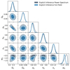 |
Fig. A.1. From log-normal simulated convergence maps at LSST Y10 quality we constrain the wCDM parameters using different inference techniques: power spectrum analysis (gray) and full-field analysis performed by sampling the forward model using an HMC sampler (blue). |
Appendix B: Implicit inference benchmark
B.1. Methods
B.1.1. Learning the likelihood ratio
Neural ratio estimation (NRE) is based on the well-known likelihood ratio test. The idea is to test whether x has been generated by θ0 or θ1 through the following quantity:
 (B.1)
(B.1)
Using the likelihood ratio trick this test can be cast as a binary classification problem where we train a classifier dφ to learn the probability that x has been generated by θ0:
 (B.2)
(B.2)
 (B.3)
(B.3)
with the two labels y = 0 and y = 1 corresponding respectively to x∼p(x|θ1) and x∼p(x|θ0).
Finally, this is generalized to all possible parameters θ by defining the label y = 0 as (x,θ)∼p(x)p(θ) and the label y = 1 corresponding to (x,θ)∼p(x,θ). This means that now the classifier learns
 (B.4)
(B.4)
leading to the following likelihood ratio
 (B.5)
(B.5)
Durkan et al. (2020) generalized this binary classification into a K multi-class classification and showed performance improvement when K>2.
Similarly to NLE, given observed data x0, the approximated posterior is then obtained by sampling the distribution.
B.1.2. Learning the posterior
Neural posterior estimation (NPE) aims to directly learn the posterior distribution. Similarly to NLE, NPE is based on neural density estimators such as NFs, whose goal is to learn pφ(θ|x) from a set of parameters and corresponding simulations (θ,x)i = 1..N. This can be done by using a conditional NF and minimizing DKL:
![Mathematical equation: $$ {\hat {\varphi }} = \arg \min _{\varphi } {\mathbb {E}}_{p(x)} \left [D_{KL}(p(\theta |x) \; || \; p_{\varphi }(\theta |x)) \right ], $$](/articles/aa/full_html/2025/07/aa52410-24/aa52410-24-eq54.gif) (B.6)
(B.6)
![Mathematical equation: $$ \implies {\cal {{L}}} = {\mathbb {E}}_{p(\theta , x)} \left [- \log p_{\varphi } (\theta |x) \right ]. $$](/articles/aa/full_html/2025/07/aa52410-24/aa52410-24-eq55.gif) (B.7)
(B.7)
Note that, unlike NLE and NRE, for NPE no MCMC is needed to get samples from the posterior. This approach is very convenient if one has to evaluate the posterior distribution for different observations as it only requires a new evaluation of the learned model pφ(θ|x).
B.2. Sequentially refined posterior
In most cases the prior p(θ) is significantly broader compared to the posterior p(θ|x=x0), making it unnecessary to sample the entire parameter space. Instead, we would like to sample from a proposal  which denotes the most suitable regions. The question arises: How to choose this proposal
  if we know neither the posterior location nor its size?
Starting from the prior, sequential methods offer a way to iteratively select this proposal by using the previous posterior approximation as the new relevant area and consequently refining the posterior at each iteration.
Each of the methods described above (NPE, NLE, and NRE) can be sequentially adjustable, however, there are some specificities to bear in mind: both SNLE (Papamakarios et al. 2018) and SNRE (Durkan et al. 2020; Hermans et al. 2020) necessitate a sampling method or variational inference (Glöckler et al. 2022; Wiqvist et al. 2021) at the end of each iteration to obtain the new parameters θ. SNPE (Papamakarios & Murray 2018; Lueckmann et al. 2017; Greenberg et al. 2019; Deistler et al. 2022) usually requires a costly correction of the approximated posterior since now minimizing the loss from Eq. B.7 under the proposal  leads to
 (B.8)
(B.8)
B.3. Results
To benchmark (S)NLE, (S)NPE, and (S)NRE methods, we use the same benchmark procedure as the one presented in Sect. 6. We use the sbi package for (S)NPE, (S)NLE, and (S)NRE methods. We choose to rely on sbi's developers’ expertise and use the default setting of sbi but optimizing the architectures would be interesting future work. For now, more detail about the implementation of these algorithms can be found in Appendix D.4.
Our numerical results in Fig. B.1, suggest that NPE and NLE methods perform the best. The results also show that the sequential methods outperform their nonsequential analog. In particular, we find that SNPE and SNLE are the methods to favor as they allowed us to achieve a posterior quality of 0.6 with only 1 000 simulations.
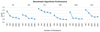 |
Fig. B.1. Implicit inference: quality of the cosmological posterior approximation as a function of the number of simulations used. We compare six methods using the default implementation of the sbi package: NLE, NPE, NRE, and their sequential counterparts SNLE, SNPE, and SNRE. |
Appendix C: MSE minimization
In this section we demonstrate that the following loss function
![Mathematical equation: $$ \begin{aligned} {\cal {{L}}} &= {\mathbb {E}}_{p(x,z,\theta )} \left [\parallel g(x, \theta , z) - g_\varphi (x,\theta ) \parallel _2^2 \right ], \end{aligned} $$](/articles/aa/full_html/2025/07/aa52410-24/aa52410-24-eq60.gif)
is minimized ∀(x,θ)∼p(x,θ) by
![Mathematical equation: $$ \begin{aligned} g_\varphi (x,\theta ) = {\mathbb {E}}_{p(z | x,\theta )} \left [g(x, \theta , z) \right ]. \end{aligned} $$](/articles/aa/full_html/2025/07/aa52410-24/aa52410-24-eq61.gif)
This proof is inspired by Remy (2023).
The optimal parameters of neural networks are typically chosen to cancel the following gradient:
![Mathematical equation: $$ \begin{aligned} \frac {\partial {\cal {{L}}}}{\partial \varphi } &= \frac {\partial }{\partial \varphi } \; {\mathbb {E}}_{p(x,z,\theta )} \left [\parallel g(x, \theta , z) - g_\varphi (x,\theta ) \parallel _2^2 \right ]\\ &= \frac {\partial }{\partial g_\varphi } \; {\mathbb {E}}_{p(x,z,\theta )} \left [\parallel g(x, \theta , z) - g_\varphi (x,\theta ) \parallel _2^2 \right ] \times \frac {\partial g_\varphi }{\partial \varphi }. \end{aligned} $$](/articles/aa/full_html/2025/07/aa52410-24/aa52410-24-eq62.gif)
Since gφ is by construction very unlikely to have null derivatives with respect to its parameters it means that
![Mathematical equation: $$ \begin{aligned} \frac {\partial }{\partial g_\varphi } \; {\mathbb {E}}_{p(x,z,\theta )} \left [\parallel g(x, \theta , z) - g_\varphi (x,\theta ) \parallel _2^2 \right ] = 0. \end{aligned} $$](/articles/aa/full_html/2025/07/aa52410-24/aa52410-24-eq63.gif)
Thanks to Leibniz integral rule we can switch the gradient and integrals such that
![Mathematical equation: $$ \begin{aligned} {\mathbb {E}}_{p(x,z,\theta )} \left [\frac {\partial }{\partial g_\varphi } \parallel g(x, \theta , z) - g_\varphi (x,\theta ) \parallel _2^2 \right ] &= 0\\ {\mathbb {E}}_{p(x,z,\theta )} \left [-2 \; g(x, \theta , z) + 2 \; g_{\varphi }(x,\theta )\right ] &= 0\\ {\mathbb {E}}_{p(x,\theta )} \left [-2 {\mathbb {E}}_{p(z| x,\theta )} \left [\; g(x, \theta , z)\right ] + 2 \; g_{\varphi }(x,\theta )\right ] &= 0. \end{aligned} $$](/articles/aa/full_html/2025/07/aa52410-24/aa52410-24-eq64.gif)
As ![Mathematical equation: $ {\mathbb {E}}_{p(x,z,\theta )} \left [\parallel g(x, \theta , z) - g_\varphi (x,\theta ) \parallel _2^2\right ] $](/articles/aa/full_html/2025/07/aa52410-24/aa52410-24-eq65.gif) is convex with respect to gφ, it has a unique minimum that is reached when
is convex with respect to gφ, it has a unique minimum that is reached when
![Mathematical equation: $$ \begin{aligned} g_\varphi (x,\theta ) = {\mathbb {E}}_{p(z | x,\theta )} \left [g(x, \theta , z) \right ]. \end{aligned} $$](/articles/aa/full_html/2025/07/aa52410-24/aa52410-24-eq66.gif)
Appendix D: Experiments additional information
Codes for the compressor, the forward model, and the explicit full-field analysis are available at sbi_lens. All codes relative to the benchmark of implicit inference techniques are available at sbi_bm_lens.
D.1. Compressor acrchitecture
To compress the convergence maps of 5×256×256 pixels into a 6 dimensional summary statistics we used a residual neural network (ResNet) (He et al. 2016) architecture. Specifically the ResNet-18. The ResNet-18 was trained under the VMIM loss function as described in Sect. 6.3.
D.2. Neural network architecture to learn marginal gradients
To learn the marginal gradients ∇θp(x |θ) from the joint stochastic one ∇θp(x,z |θ) provided by the simulator, we used a neural network with 2 layers of 256 hidden units and Leaky ReLU activation functions. To test that we learned the correct marginal gradients we compared them against the gradients of a conditional NF trained with 105 simulations under the NLE loss.
D.3. NLE and ∂NLE architectures
For this study, the NF architecture remains fixed for the two methods, only the input changes: 1) we used only simulations; 2) we used simulations and the gradients of the simulator; 3) we used the simulations and the learned marginal gradients. Our conditional NF is a RealNVP (Dinh et al. 2017) of 4 coupling layers. Scale and shift parameters are learned using a neural network of 2 layers of 128 hidden units each. We used SiLU activation functions. To get the posterior from the learned likelihood, we used NUTS sampler. The epistemic uncertainty is approximated by training 7 NFs.
D.4. Standard implicit inference architectures
To compare all the implicit inference techniques, we used the sbi package for (S)NPE, (S)NLE and (S)NRE methods.
For the sequential approach, the simulation budget was split across 5 rounds. To approximate the epistemic uncertainty we trained 5 NFs for each simulation budget.
(S)NLE. We used Papamakarios et al. (2018) version of NLE and SNLE algorithm. In line with previous works (Durkan et al. 2020; Papamakarios et al. 2018; Lueckmann et al. 2021; Greenberg et al. 2019), our neural density estimator is a Masked Autoregressive Flow (MAF) (Papamakarios et al. 2017) with 5 autoregressive layers, each has two hidden layers of 50 units each. We used Tanh activation functions. Still in line with previous works, we used Slice Sampling schemes to recover the posterior distribution. Note that this is not the most efficient MCMC to explore high-dimensional or multi-modal spaces. However, since we are in a 6 almost Gaussian dimensional space this scheme works very well.
(S)NPE. We used NPE algorithm as formulated in Papamakarios & Murray (2018) but used as a neural density estimator a MAF instead of a Mixture Density Network (MDN). For SNPE algorithm we use Automatic Posterior Transformation (APT) by Greenberg et al. (2019). In line with previous works, our neural density estimator is a MAF with 5 autoregressive layers, each has two hidden layers of 50 units each. We used Tanh activation functions. For APT, to compute the atomic proposal, we used M = 10 atoms. The computational complexity of APT is O(M2) and as underlined by Lueckmann et al. (2021) more atoms are very demanding in terms of memory. In addition, unlike Greenberg et al. (2019) we found a difference in training time between M = 10 and M = 100 atoms.
Even though APT outperforms previous sequential NPE methods (Papamakarios & Murray 2018; Lueckmann et al. 2017), as reported by the APT paper itself Greenberg et al. (2019) and Durkan et al. (2020), this algorithm can suffer from leakage of posterior mass outside the prior support. To overcome this issue Deistler et al. (2022) introduced Truncated Sequential Neural Posterior Estimation (TSNPE).
(S)NRE. We used NRE algorithm as in Durkan et al. (2020) and used K = 10 class. In line with previous works (Durkan et al. 2020; Lueckmann et al. 2021), the K multi-class classifier is a residual neural network with two residual blocks of 50 hidden units and ReLU activation functions. Still in line with previous works, we used Slice Sampling schemes to recover the posterior distribution.
Appendix E: Additional convergence plots
We provide additional results showing the convergence of inference methods. Figure E.1 shows the contours evolution of the implicit inference posteriors approximated with NLE method. Figures E.2, E.4, E.3, and E.5 show the evolution of the approximated mean and standard deviation of the posteriors approximated with NLE, ∂NLE with joint gradients and marginal gradient, and the explicit inference methods. Figure E.6 shows the contours evolution of the explicit inference posterior. Finally, Fig. E.7 displays the KDE approximation used to compute the C2ST metric of explicit inference method.
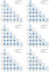 |
Fig. E.1. Evolution of implicit inference posteriors according to the number of simulations used to train the NF. The posteriors (blue contours) are approximated using the NLE method with simulations only. We train 5 NFs with the same architecture where only the initialization of the weights of the NF changes. Each blue contours correspond to the approximated posterior of one of these NFs. The ground truth (black contours) corresponds to the explicit inference posterior of 160 000 samples and the black marker corresponds to its mean. The yellow marker corresponds to the mean of the approximated posterior. With few simulations (e.g. 100 simulations) every NF predicts a different posterior and each prediction is overconfident. With a bit more simulations (e.g. 1 000 simulations), the posteriors are consistent and similar to the ground truth. |
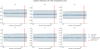 |
Fig. E.2. Evolution of the mean and standard deviation of the approximated implicit inference posterior as a number of simulations. The posterior is approximated using the NLE method with only simulations. We train five NFs with the same architecture where only the initialization of the weights of the NF changes. The blue line corresponds to the mean of the five approximated posteriors and the dotted line to the standard deviation. The dashed line corresponds to the mean of the ground truth (the explicit inference posterior of 160 000 samples), and the black dotted line to its standard deviation. The red line corresponds to the number of simulations for which the C2ST is equal to 0.6 (i.e. assume that the posterior is converged). Note that the C2ST can compare ”higher moments” than the first and second moments of two distributions thus these plots cannot serve as direct conclusions. |
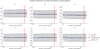 |
Fig. E.3. Same as the previous figure but this time the posterior is approximated using the ∂NLE method with simulations and gradients. |
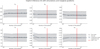 |
Fig. E.4. Same as the previous figure but this time the posterior is approximated using the ∂NLE method with simulations and marginal gradients. |
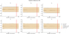 |
Fig. E.5. Evolution of the mean and standard deviation of the explicit inference posterior as a number of simulations. To get our 160 000 posterior samples (our ground truth) we use the NUTS algorithm. For each simulation budget N, we select the first N samples of this ground truth and compute its mean and standard deviation. The yellow line and dotted line correspond respectively to the mean and standard deviation. The black dashed line corresponds to the mean of the ground truth (of 160 000 posterior samples), and the black dotted line to its standard deviation. The red line corresponds to the number of simulations for which the C2ST is equal to 0.6 (i.e. assume that the posterior is converged). Note that the C2ST can compare ”higher moments” than the first and second moments of two distributions thus these plots cannot serve as direct conclusions. |
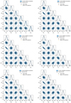 |
Fig. E.6. Evolution in terms of simulations of the explicit inference approximated posterior. The ground truth (black contours) corresponds to the explicit inference posterior of 160 000 samples. The blue contours denote the first N samples of the ground truth. Note that to get one sample our NUTS algorithm requires 126 simulations. The black marker corresponds to the mean of the ground truth. The yellow one, to the mean of the approximated posterior. |
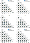 |
Fig. E.7. Samples of the KDE used to compute C2ST metric. In this paper we use the C2ST metric to evaluate the convergence of inference methods. This metric requires an equal number of simulations of the two distributions to be compared. To use the C2ST metric to benchmark the explicit inference method, inspired by the construction of contour plots that smooth the distribution (such as the one proposed by GetDist), we use a KDE to generate new samples. Specifically, we use a Gaussian kernel and set the bandwidth to match what GetDist would display for every number of explicit inference posterior samples (black contours). The yellow contours correspond to the contours obtained when fitting the N samples of explicit inference posterior and generating 20 000 samples from the KDE. We use a very small smoothing scaling value to display the posterior contours of the KDE with GetDist. The blue contours denote the ground truth of 160 000 samples. |
All Tables
All Figures
|
Fig. 1. Example of noisy convergence map, with five tomographic redshift bins, generating with sbi_lens's log-normal forward model. It is the fiducial map x0 used for benchmarking all the inference techniques. |
| In the text | |
|
Fig. 2. Representation of sbi_lens's forward model used to generate log-normal convergence maps. |
| In the text | |
|
Fig. 3. LSST Y10 redshift distribution used in our forward model. |
| In the text | |
|
Fig. 4. From log-normal simulated LSST Y10-like convergence maps, we constrain wCDM parameters using two approaches: (1) the explicit full-field inference (black), obtained by sampling 160 000 posterior samples through an HMC scheme; and (2) the implicit full-field inference contours (blue), obtained by compressing the convergence maps into sufficient statistics using variation mutual information maximization (VMIM) and performing inference using NLE with 1000 simulations. We show three things: (1) implicit and explicit full-field inferences yield consistent constraints; (2) our implicit inference, when combined with an optimal compression procedure, allows full-field inference; (3) the C2ST metric indicates convergence when it is equal to 0.5 (see Sect. 4). However, when comparing explicit and implicit inference (which should theoretically yield the same posterior), we never reach this value, but rather we obtain 0.6. We justify that this value is acceptable and use it as a threshold for all benchmarked methods in this paper by showing that the marginals of the two approaches match, even though their C2ST is 0.6. |
| In the text | |
|
Fig. 5. Explicit full-field inference: quality of cosmological posterior approximation as a function of the number of simulations used and effective sample size. The dashed line indicates the C2ST threshold of 0.6, marking the point at which the posterior is considered equal to the true distribution (see Sect. 4). |
| In the text | |
|
Fig. 6. Implicit inference augmented with gradients: quality of the cosmological posterior approximation as a function of the number of simulations used. We compare three methods: (1) ∂NLE with the gradients of the simulator ∇θlog p(x,z|θ) (yellow); (2) ∂NLE with marginal gradients ∇θlog p(x|θ) (blue); and (3) the classical NLE method (black). The dashed line indicates the C2ST threshold of 0.6, marking the point at which the posterior is considered equal to the true distribution (see Sect. 4). We show that the gradients provided by the simulator (yellow curve) do not help reduce the number of simulations as they are too noisy (see Fig. 7). |
| In the text | |
|
Fig. 7. Illustration of gradient stochasticity. The left panel shows a 2D posterior distribution p(θ|x=x0) evaluated at the observed data x0 and its gradients ∇θlog p(θ|x=x0). The middle panel shows the difference between the posterior p(θ|x=x0) (yellow) and the joint posterior p(θ|x=x0,z=z0) (blue) with z0 a latent variable that leads to x0. The yellow arrows correspond to the gradients of the posterior, and the blue ones to the gradients of the joint posterior. The right panel displays the gradient field that we obtained in practice from the simulator. Each gradient aligns with its corresponding joint posterior, resulting in a “noisy” gradient field compared to that of the posterior (first panel). |
| In the text | |
|
Fig. A.1. From log-normal simulated convergence maps at LSST Y10 quality we constrain the wCDM parameters using different inference techniques: power spectrum analysis (gray) and full-field analysis performed by sampling the forward model using an HMC sampler (blue). |
| In the text | |
|
Fig. B.1. Implicit inference: quality of the cosmological posterior approximation as a function of the number of simulations used. We compare six methods using the default implementation of the sbi package: NLE, NPE, NRE, and their sequential counterparts SNLE, SNPE, and SNRE. |
| In the text | |
|
Fig. E.1. Evolution of implicit inference posteriors according to the number of simulations used to train the NF. The posteriors (blue contours) are approximated using the NLE method with simulations only. We train 5 NFs with the same architecture where only the initialization of the weights of the NF changes. Each blue contours correspond to the approximated posterior of one of these NFs. The ground truth (black contours) corresponds to the explicit inference posterior of 160 000 samples and the black marker corresponds to its mean. The yellow marker corresponds to the mean of the approximated posterior. With few simulations (e.g. 100 simulations) every NF predicts a different posterior and each prediction is overconfident. With a bit more simulations (e.g. 1 000 simulations), the posteriors are consistent and similar to the ground truth. |
| In the text | |
|
Fig. E.2. Evolution of the mean and standard deviation of the approximated implicit inference posterior as a number of simulations. The posterior is approximated using the NLE method with only simulations. We train five NFs with the same architecture where only the initialization of the weights of the NF changes. The blue line corresponds to the mean of the five approximated posteriors and the dotted line to the standard deviation. The dashed line corresponds to the mean of the ground truth (the explicit inference posterior of 160 000 samples), and the black dotted line to its standard deviation. The red line corresponds to the number of simulations for which the C2ST is equal to 0.6 (i.e. assume that the posterior is converged). Note that the C2ST can compare ”higher moments” than the first and second moments of two distributions thus these plots cannot serve as direct conclusions. |
| In the text | |
|
Fig. E.3. Same as the previous figure but this time the posterior is approximated using the ∂NLE method with simulations and gradients. |
| In the text | |
|
Fig. E.4. Same as the previous figure but this time the posterior is approximated using the ∂NLE method with simulations and marginal gradients. |
| In the text | |
|
Fig. E.5. Evolution of the mean and standard deviation of the explicit inference posterior as a number of simulations. To get our 160 000 posterior samples (our ground truth) we use the NUTS algorithm. For each simulation budget N, we select the first N samples of this ground truth and compute its mean and standard deviation. The yellow line and dotted line correspond respectively to the mean and standard deviation. The black dashed line corresponds to the mean of the ground truth (of 160 000 posterior samples), and the black dotted line to its standard deviation. The red line corresponds to the number of simulations for which the C2ST is equal to 0.6 (i.e. assume that the posterior is converged). Note that the C2ST can compare ”higher moments” than the first and second moments of two distributions thus these plots cannot serve as direct conclusions. |
| In the text | |
|
Fig. E.6. Evolution in terms of simulations of the explicit inference approximated posterior. The ground truth (black contours) corresponds to the explicit inference posterior of 160 000 samples. The blue contours denote the first N samples of the ground truth. Note that to get one sample our NUTS algorithm requires 126 simulations. The black marker corresponds to the mean of the ground truth. The yellow one, to the mean of the approximated posterior. |
| In the text | |
|
Fig. E.7. Samples of the KDE used to compute C2ST metric. In this paper we use the C2ST metric to evaluate the convergence of inference methods. This metric requires an equal number of simulations of the two distributions to be compared. To use the C2ST metric to benchmark the explicit inference method, inspired by the construction of contour plots that smooth the distribution (such as the one proposed by GetDist), we use a KDE to generate new samples. Specifically, we use a Gaussian kernel and set the bandwidth to match what GetDist would display for every number of explicit inference posterior samples (black contours). The yellow contours correspond to the contours obtained when fitting the N samples of explicit inference posterior and generating 20 000 samples from the KDE. We use a very small smoothing scaling value to display the posterior contours of the KDE with GetDist. The blue contours denote the ground truth of 160 000 samples. |
| In the text | |
Current usage metrics show cumulative count of Article Views (full-text article views including HTML views, PDF and ePub downloads, according to the available data) and Abstracts Views on Vision4Press platform.
Data correspond to usage on the plateform after 2015. The current usage metrics is available 48-96 hours after online publication and is updated daily on week days.
Initial download of the metrics may take a while.