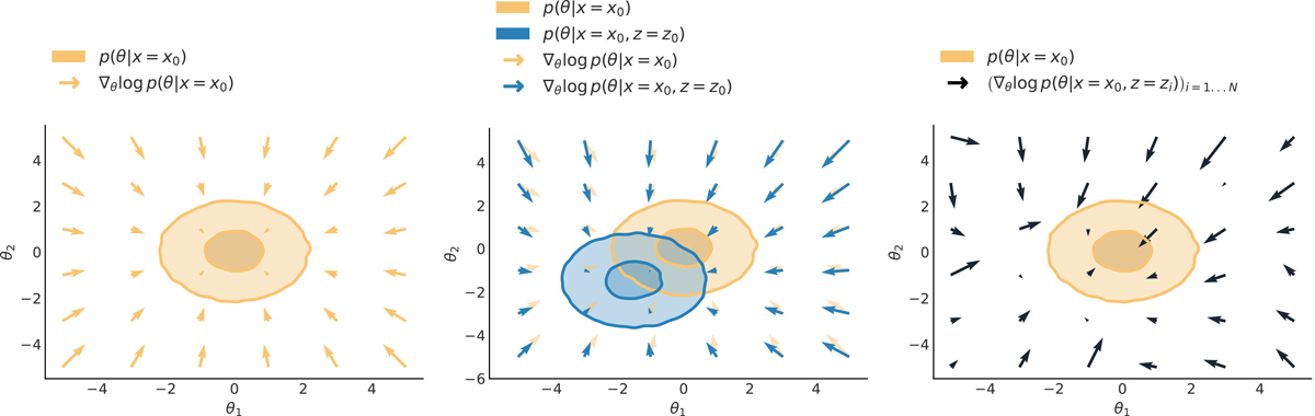
Illustration of gradient stochasticity. The left panel shows a 2D posterior distribution p(θ|x=x₀) evaluated at the observed data x₀ and its gradients ∇_θlog p(θ|x=x₀). The middle panel shows the difference between the posterior p(θ|x=x₀) (yellow) and the joint posterior p(θ|x=x₀,z=z₀) (blue) with z₀ a latent variable that leads to x₀. The yellow arrows correspond to the gradients of the posterior, and the blue ones to the gradients of the joint posterior. The right panel displays the gradient field that we obtained in practice from the simulator. Each gradient aligns with its corresponding joint posterior, resulting in a “noisy” gradient field compared to that of the posterior (first panel).